Remote Sensing Analysis to Quantify Change in Woodland Canopy Cover on the San Carlos Apache Reservation, Arizona, USA (1935 vs. 2017)


Western Geographic Science Center, U.S. Geological Survey, 520 N. Park Ave., Tucson, AZ 85719, USA
*
Author to whom correspondence should be addressed.
Land 2021, 10(4), 393; https://0-doi-org.brum.beds.ac.uk/10.3390/land10040393
Submission received: 8 January 2021
/
Revised: 2 April 2021
/
Accepted: 7 April 2021
/
Published: 9 April 2021
(This article belongs to the Section Landscape Ecology)
Abstract
:Since the late 1800s, pinyon–juniper woodland across the western U.S. has increased in density and areal extent and encroached into former grassland areas. The San Carlos Apache Tribe wants to gain qualitative and quantitative information on the historical conditions of their tribal woodlands to use as a baseline for restoration efforts. At the San Carlos Apache Reservation, in east-central Arizona, large swaths of woodlands containing varying mixtures of juniper (Juniperus spp.), pinyon (Pinus spp.) and evergreen oak (Quercus spp.) are culturally important to the Tribe and are a focus for restoration. To determine changes in canopy cover, we developed image analysis techniques to monitor tree and large shrub cover using 1935 and 2017 aerial imagery and compared results over the 82-year interval. Results showed a substantial increase in the canopy cover of the former savannas, and encroachment (mostly juniper) into the former grasslands of Big Prairie. The Tribe is currently engaged in converting juniper woodland back into an open savanna, more characteristic of assumed pre-reservation conditions for that area. Our analysis shows areas on Bee Flat that, under the Tribe’s active restoration efforts, have returned woodland canopy cover to levels roughly analogous to that measured in 1935.
1. Introduction
Among the most widespread and dramatic vegetation changes to occur since the late 1800s in the western United States is the expansion and increase in density of juniper (Juniperus spp.) and pinyon (Pinus spp.) trees [1,2,3,4,5,6,7,8,9,10]. In the American West, pinyon–juniper woodlands are estimated to have increased in areal extent from ~3 to ~30 million ha (19th century estimate/end of 20th century estimate) [5,9,11,12] and have encroached into former grassland areas. In the western state of Arizona, pinyon–juniper woodland is the dominant woodland/forest vegetation type [13,14], covering more area than all forest types combined [14]. Former savanna areas dominated by native grasses and forbs were replaced with higher-density pinyon–juniper woodlands, with the degraded soils and herbaceous understories that are often associated with them [15]. Periodic fire in these historical savanna environments had resulted in the low density of trees. Historically, higher-density woodlands were confined to rocky ridges, hillslopes, and flats where grasses were discontinuous and fine fuels were insufficient to carry fires [5,6,7,13,15,16,17].
A mission of the San Carlos Apache Tribe is to attempt to restore reservation lands to pre-reservation (pre-1872) conditions. The Tribe has an interest in learning more about the historical characteristics of their woodlands, savannas, and grasslands so that they have a target for restoration goals. It is hypothesized that in pre-reservation times, the woodland distribution and cover were different than today. Sites had more continuous cover of native grasses and forbs, with frequent, widespread fires maintaining savannas and grasslands [5,7,13,15]. Savannas exist through time because fire kills the younger, smaller trees and saplings [5,7,13,15]. Tribal elders have noted that the woodland, savanna, and grassland distribution and characteristics have changed markedly within their lifetimes.
Increases in woodland tree cover and grassland encroachment by juniper, and their associated effects on reducing intercanopy herbaceous vegetation, are issues that the Tribe are coping with. The effects of increased tree cover can form a feedback cycle and include reduced amount and diversity of herbaceous cover (especially grass) that normally supported surface fires, and accelerated soil erosion in intercanopy areas partially a result of more bare ground and increased surface water runoff [1,2,5,7,8,9,12,13,18,19,20]. Livestock and wildlife often depend upon the grass cover to survive and thrive. Restoring woodland to savanna is a focus of the Tribe’s intensive management activities, and spatial information that would help to determine where best to apply restoration efforts is needed. Information and maps detailing former and current woodland tree canopy cover on the reservation would be an important component to the Tribe’s management information needs.
Our remote sensing research explores how the canopy cover of woodlands changed on the San Carlos Apache Reservation, Arizona, since 1935, and whether woodland trees (i.e., juniper) have encroached into former grasslands on the reservation. We developed image analysis techniques to create maps that document change in the tree and large shrub cover over an 82-year interval. Aerial photography from 1935 (Fairchild Aerial Surveys) was compared to digital imagery from the 2017 National Agriculture Imagery Program (NAIP). The earliest, large-scale aerial photography for the area was from 1935 and was used to generate historical baseline and change information. These maps provide insight into the change in woodland tree/large shrub canopy cover as well as woodland tree encroachment into former grasslands. Woodland areal extent (i.e., hectares of woodland) was not quantified. Study areas within the reservation were selected based upon the observed presence of woodland, savanna, and grassland in 2017, in conjunction with the postulated existence of these cover types in 1935. The study sites were, therefore, not ideal for looking at changes in areal extent.
2. Materials and Methods
2.1. Study Area
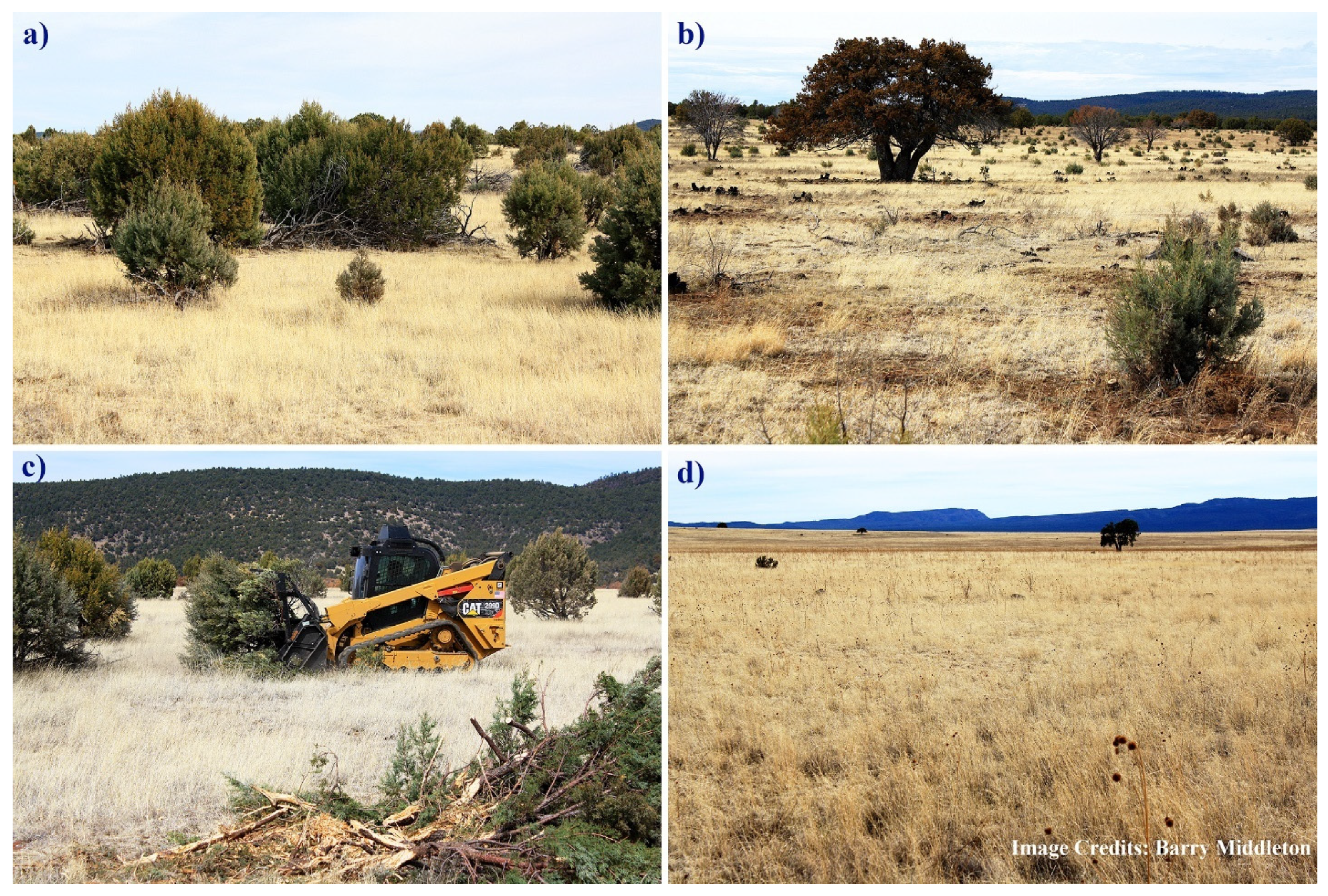
Woodlands containing varying mixtures of juniper (Juniperus spp.), pinyon (Pinus spp.) and, uniquely, evergreen oak (Quercus spp.) cover a considerable part of the northern San Carlos Apache Reservation [21] and are important culturally to the Tribe (Figure 1a–d). This woodland community is sometimes referred to as Madrean pinyon–juniper woodland. Woodlands, depending on their condition, can offer food (pinyon nuts and Emory oak acorns, etc.), fuelwood, wildlife habitat, livestock forage, and watershed protection and services [13], in addition to other cultural resources and landscape important to the Apache people.
The San Carlos Apache Reservation vegetation represents a transition between the more cold-tolerant Great Basin Conifer Woodland (pinyon–juniper) to the north and the milder climate (warmer and wetter) represented by the Madrean Evergreen Woodland to the south [22,23]. Species such as alligator juniper (Juniperus deppeana) and Mexican pinyon (Pinus cembroides) and many evergreen oak species (Quercus spp.) are characteristic of Madrean Evergreen Woodland [22]. One-seed juniper (Juniperus monosperma) and Colorado pinyon (Pinus edulis) are more characteristic of the Great Basin Conifer Woodland [22]. All these listed woodland tree species can be found in this region, making the pinyon–juniper–evergreen oak woodlands on the reservation somewhat unique. The evergreen oak species present in the study areas are primarily Arizona white oak (Quercus arizonica). Additionally, some groves of Emory oak (Quercus emoryi) can be found in drainages and, together with their acorns, are a very important culinary and cultural resource to the Tribe. For this project, we will often refer to the woodland trees delineated in the maps as “trees/large shrubs.” This designation highlights that the tree species are found in an array of sizes and that trees and larger saplings are both included in the mapping efforts. Although large shrub species (i.e., manzanita, mountain-mahogany, etc.) are found sometimes in these woodlands, they are not nearly as common as larger saplings of juniper, pinyon, and evergreen oaks.
Pinyon–juniper–evergreen oak woodland and juniper savanna are interspersed with grasslands, evergreen oak woodlands, and ponderosa pine forest in the region [21,23]. There are other major vegetation types within the study areas that include ponderosa pine (Pinus ponderosa) and, as seen at Big Prairie, continuous grassland. Oak woodlands to the south of the study areas also intergrade over long distances with pinyon–juniper woodland on the reservation creating unique plant assemblages. In general, for pinyon–juniper and juniper woodland or savanna, as elevation and precipitation increases, pinyon increases in dominance while juniper decreases, total tree density increases, and trees become larger [13]. At the lowest elevations, junipers occur without pinyon [13,22]. Juniper is more drought tolerant than pinyon [13,16,24] and can be found in relative monoculture at more xeric sites [22], or along with pinyon and evergreen oak (and even ponderosa pine) under more mesic conditions. The greatest diversity, density and tree size in the woodland tree cover are often achieved near its upper elevational limit with ponderosa pine [13]. The diversity of herbaceous plants is much greater than the woodland tree diversity and plays a major role in differentiating woodland vegetation types [25]. It is often the presence or absence of key understory species that is used to determine the specific woodland type [25].
In this paper, pinyon–juniper–evergreen oak woodland is meant to define a transitional woodland with juniper, pinyon, and evergreen oak in varying mixtures. Juniper woodlands found in the drier, lower elevations are considered along with woodlands also containing pinyon and/or evergreen oak species. A vast majority of the pinyon–juniper and juniper woodlands in the Intermountain West, however, occurs without evergreen oaks. The Madrean oak species are more characteristic and common in the United States in southeastern Arizona, southern New Mexico, and west Texas [22]. We are considering savanna to have woodland trees with a canopy cover up to 15% and grassland to be continuous, large areas of herbaceous plant cover mostly devoid of trees.
Three, large woodland study areas (Bee Flat, Big Prairie and Bloody Basin) ranging in area between 146 and 220 km2 (56 and 85 mi2) in the northern portion of the San Carlos Apache Reservation are selected by the Tribe for case studies (Figure 2). They are all north of the NW-SE trending Natanes Rim on an elevated plateau. All three study areas extend north across the Black River and into the reservation of the White Mountain Apache Tribe, bordering to the north, although the majority of all three are on the San Carlos Apache Reservation. The Black River divides the northern boundary of the San Carlos Apache Reservation from the southern boundary of the White Mountain Apache Reservation. The three study areas (Bee Flat, Big Prairie and Bloody Basin; Figure 2) selected by the San Carlos Apache Tribe for this analysis are considered to contain good examples of woodland dominated by juniper, pinyon, and evergreen oak. Additionally, the Big Prairie study area is selected because it currently contains a long interface between woodland and grassland vegetation types. This study area is where the encroachment of woodland trees into former grassland areas can be readily examined.
2.1.1. Bee Flat
The majority of the Bee Flat study area is woodland with some limited ponderosa pine and riparian forest along the Black River (Figure 2). The central portion of the Bee Flat study area includes a large area of on-going, intensive woodland management. The Tribe is engaged in removal of woodland juniper trees to create a more open savanna-type environment, more characteristic of hypothesized pre-reservation (pre-1872) conditions. These managed areas have been (and are being) mechanically treated to remove juniper trees and increase the potential area for herbaceous cover and are targeted at creating a functioning savanna from a woodland environment. The success of the restoration efforts, of course, depends on the longer-term success of tree removal and a host of necessary site characteristics (i.e., soil, vegetative, and hydrologic, etc.) for herbaceous plant growth and success. Mastication (shredding) is the current technique being employed, although smaller areas of cutting and chaining occur in this study area in the past. Herbicides to assist in killing the junipers have also been applied in conjunction with some of these mechanical treatments (Figure 3a–c). Evidence of relatively recent fire can also be discerned in the 2017 imagery in the north and west parts of the study area.
2.1.2. Big Prairie
The Big Prairie study area covers the northwest portion of the grasslands known as Big Prairie, and surrounding woodlands and forest (ponderosa pine and riparian) to the west and north (Figure 2 and Figure 3d). Big Prairie is a large, natural grassland area in the northeast part of the San Carlos Apache Reservation (near Point of Pines) and is mostly devoid of trees except around the periphery. A large portion of this continuous high-elevation (approximately 1830 m (6000 ft.)) grassland covers the eastern half of the study area. Historical and more recent smaller-scale woodland treatment areas can be found here and seen on the imagery. Fire scars in the western part can also be discerned, with the Creek Fire in 2013 burning a large portion of the ponderosa pine forest (and some dense woodland) that originally covers some of the southwestern part of the study area.
2.1.3. Bloody Basin
Bloody Basin is a remote and very dense woodland area (Figure 2). It had some active woodland management (chaining) back in the 1960s, but the area treated was relatively modest as compared to the treatment area on Bee Flat. The historical chaining seems to have occurred in the vicinity of Bloody Basin Tank near the middle of the study area. (Note: The location of this stock tank will be shown more precisely later in the paper) Limited ponderosa pine, and riparian forest along the Black River, are also found in the study area.
2.2. Methodology
Object-oriented/image segmentation approaches are currently favored to map canopy cover of trees [4,9,19,20,26], although pixel-based classification and thresholding techniques have been employed as well [26,27]. We chose to use a unique pixel-based approach for this study because (1) the iterative nature of the approach allowed nearly immediate feedback on the canopy selection and (2) we think previous pixel-based approaches could be improved upon, especially in reference to spurious pixels (“salt and pepper effect”) when using high spatial resolution data. This approach fundamentally focuses on the color space of the pixels in a series of 3-band images to determine whether the pixel belongs to the canopy or not. It is best classified as a pixel-based, supervised classification although it is non-traditional in that the input pixel information is a reference color and the operator assisted classification is run by the algorithm based on pixel color space information. We tried to identify and map the tree canopies, including basic supervised classifications of the 5-band layer stack (red, green, blue, NIR, Normalized Difference Vegetation Index (NDVI)) in ERDAS Imagine. Our results were less than satisfactory, with the full tree canopies not completely mapped and tree shadows falling on the ground not being isolated from the shadows in the canopy itself. We introduce a novel pixel-based methodology to map canopy cover using Adobe Photoshop and ERDAS Imagine.
The methodology for processing the 2017 aerial digital imagery and the digitized 1935 aerial photography is described below and graphically summarized in Figure 4. The techniques used in the delineation of the tree/large shrub canopy maps are unique to this project and are described in detail. Associated figures are provided to show the results of the methodology for one study area (Bee Flat) and are found at the end of this section.
2.2.1. 2017 National Agriculture Imagery Program Processing
2.2.1.1. Acquisition, Subsetting, and Band Calculation
The 2017 National Agriculture Imagery Program (NAIP) digital aerial imagery (seamless) covering the northern portion of the San Carlos Apache Reservation was downloaded from the USGS Earth Explorer website (https://earthexplorer.usgs.gov/) on 10 September 2018. The NAIP imagery was flown on 17/18 June 2017, and has a spatial resolution of 0.60 m. The bands are as follows: red = band 1, green = band 2, blue = band 3, and near infrared (NIR) = band 4. The downloaded image tiles were first mosaiced together and then clipped in ERDAS Imagine 2014 to a reference extent. It was then subsetted into the 3 study areas (Bee Flat, Big Prairie and Bloody Basin). The Normalized Difference Vegetation Index (NDVI) was calculated from the NIR and red bands of the data.
NDVI = (NIR − red)/(NIR + red)
The study area imagery, including NDVI, was then exported one band at a time from ERDAS Imagine as a TIF file. Ultimately, the 2017 imagery was displayed in 3-band color or false color images in Adobe Photoshop CC (Photoshop) after merging the individual “channels” in a specific order. Saving the bands individually was necessary as images exported from ERDAS Imagine as 3-band TIF files could not be opened in Photoshop.
2.2.1.2. Delineating Tree/Large Shrub Canopies
The first band combination chosen to highlight the tree/large shrub canopy and distinguish it from the remaining vegetation (i.e., grass, annuals, etc.) and non-vegetation (i.e., soil, rock outcrops, shadows—not falling on tree canopies, etc.) was bands 1, 4, 3 (red, NIR, blue). This band combination was displayed in Photoshop with no stretch to allow for the standardization of the following techniques across study areas.
This technique involves a specific and controlled application of Photoshop’s “Magic Wand tool” to approximately delineate tree and large shrub canopies in the 3-band false color imagery. The Magic Wand tool selects pixels based on tone and color. A green color (red, green, blue (RGB) = 0, 200, 0) close to the color of the trees in the false color imagery was selected and a very small rectangle (at 100% magnification) was drawn on the displayed image in a water body or other area that did not include tree or shrub canopies. This rectangle was then filled with this color and used in conjunction with Photoshop’s Magic Wand tool to select pixels across the image that are observed to delineate tree/large shrub canopies. The tool was used to select the rectangle, and thereby select other “like” pixels across the image, a basic supervised classification performed in Photoshop. (Note: “Anti-alias” and “Contiguous” are left unchecked.) Photoshop’s Magic Wand tool “tolerance” setting is iteratively changed until the analyst finds the resulting selection to most closely include the full tree canopies (including those in shadow). This “selection” often excluded grassland and other non-tree areas (tree shadows over exposed soil, etc.); however, the result was not entirely satisfactory. The tolerance value that was selected as best representing the entire tree canopies had a value of 205. This modification of the normal use of this powerful tool allowed the technique to be reproducible as well as efficient. While some other green vegetation was selected, a vast majority of the senescent grass was not because of the mid-June date of the imagery. Usually, mid-June is hot and dry in Arizona and a time when the perennial bunch grasses at these elevations are still dormant and awaiting the initiation of the summer monsoonal rains. Selected areas were then filled with white, while non-selected areas were filled with black. The small rectangle was then filled with black as well. This same technique (with same patch color and tolerance value of 205) was ultimately applied to the 2 other study areas, again displayed with no stretch. In general, the focus of the Magic Wand tool selection process was on fully and precisely including the tree canopy pixels, and not on the exclusion of non-canopy pixels.
A second 3-band combination image was used to further refine the selected pixels and create a second tree/large shrub canopy mask. This time the band combination used the calculated NDVI as the green band in the display, instead of NIR. The band combination was therefore 1, NDVI, 3 (red, NDVI, blue). The same green (RGB = 0, 200, 0) color was selected and a very small rectangle was delineated on the image and filled with this color, and different Magic Wand tool tolerance values attempted until tree canopies were fully and precisely selected, with senescent grass, soil and rock generally excluded. A tolerance value of ‘180′ was ultimately chosen and used to create a binary black and white image with tree canopies and other green vegetation displayed as white, and other areas, including senescent grass, soil and rock, displayed as black. This technique, including the tolerance value of 180, was applied to the two other study area images as well. Again, no stretch was applied to the imagery.
A third mask was created using the “natural or true color” band combination 1, 2, 3 (red, green, blue). This time a darker green value (RGB = 0, 100, 0) was chosen to fill the small rectangle added to the imagery as it more closely approximates the green of the trees. The Magic Wand tool tolerance value that most closely results in capturing the full tree canopy extent was ‘120’. This same methodology was applied to the other 2 study areas (displayed with no stretch) to ultimately create binary black and white image masks for each study area.
In general, the Magic Wand tool tolerance value used to create each mask is the lowest value that fully selects the tree canopies. Selecting the entire canopies resulted in the selection of more non-tree canopy pixels than wanted, but the following step greatly minimized the “unwanted” pixels while maintaining the tree canopy pixels. Ultimately, this was an iterative process.
Then, for each study area, the “intersection” of the 3 image masks derived from each of the 3-band image displays was determined in Photoshop and used as the final tree/large shrub canopy map for that study area. Intersection, in this case, was defined as the area of overlap between the selected image layers. The image layers were the 3 canopy masks generated for a single study area; and were determined by stacking the individual images and identifying the area of overlap (i.e., white pixels in common) between them. Identifying the intersection was performed in Photoshop, although it can be accomplished in other software such as ESRI’s ArcMap or ERDAS Imagine. This image intersection resulted in a more reasonable depiction of the tree canopy and non-tree canopy areas than any single mask alone (Figure 5a,b and Figure 6c).
2.2.1.3. Percent Cover Estimation
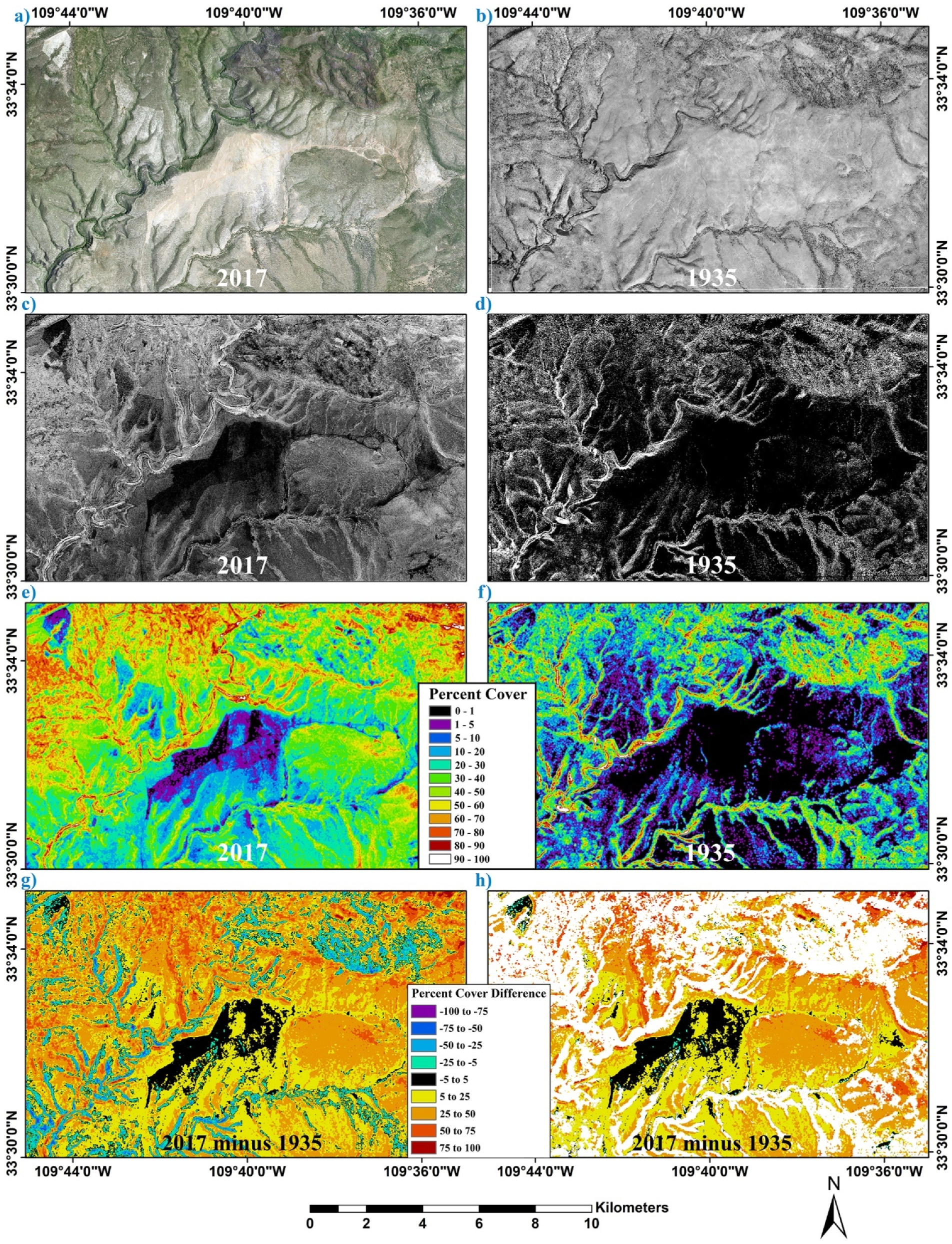
The “intersection images” (saved in TIF format) created in Photoshop were then imported back into ERDAS Imagine 2014, and map and projection information restored. The TIF format allowed the file to be used interchangeably between Photoshop and ERDAS Imagine. An unsupervised classification (2 classes) was run on each of the final study area tree/large shrub maps to classify black and white pixels into 2 classes. The former white pixels denoting tree/large shrub presence were then recoded to a value of 1, while the former black pixels were recoded to a value of 0. A model was then created in ERDAS Imagine and run to calculate a “moving window” mean value over an approximately 50 m by 50 m area (83 × 83 pixels) for each of the tree/large shrub canopy maps for the 3 study areas. The mean value was input into the central pixel of the surrounding 83 by 83 pixel “window”, and so on, as the window moved. Running the model results in an image that expressed the fractional cover, measured over an extended area representing approximately 2500 m2, of the tree and large shrub canopy over the entire study area. These fractional cover images (range 0 to 1) were multiplied by 100 to calculate percent cover (range 0 to 100). The images were then opened in ESRI’s ArcMap 10.5, and color coded into class ranges for display (Figure 6e).
2.2.2. 1935 Aerial Photography
2.2.2.1. Acquisition
We located 1935 aerial photography (Fairchild Aerial Surveys Incorporated for Soil Erosion Service, predecessor to the Soil Conservation Service) [28] at the Map and Geospatial Hub at Arizona State University. We downloaded 8 digital scans of aerial photography print mosaics, each representing roughly the same area as a 15′ topographic quadrangle (1:62,500), for the northern portion of the San Carlos Apache Reservation (Figure 2). The digital scans of the aerial photography do not come with metadata and do not have the georeferencing embedded digitally (i.e., as in a GeoTIFF file, etc.). Although the scans have latitude and longitude visually marked near all 4 corners, the date(s) flown, projection, pixel size and other important information is not recorded with the imagery. Since the individual mosaics come with very limited geometric information and without any projection or pixel size information, it would be necessary to do much more processing initially than for the “data ready” 2017 NAIP imagery.
2.2.2.2. Registration and Subsetting
The 1935 digital scans of aerial photography mosaics were first slightly rotated in Photoshop as most of the print mosaic panels were scanned askew by varying small amounts. They were then clipped to the image boundaries, as there was a very broad border surrounding the images. The interior 4 corners of each of the 1935 aerial photography mosaics were labeled with their latitude/longitude coordinates. These 4 latitude/longitude markers, along with a 1st-order polynomial transformation applied in ERDAS Imagine 2014, were used to digitally georeference the individual mosaics. The 1935 mosaics could then be compared more easily to the 2017 NAIP aerial imagery, as the 1935 image mosaics were now processed to embed digital geometric information. The individual, georeferenced digital images were then mosaiced together. Histogram matching on the overlap areas was used on all 8 images to make the larger mosaic more seamless with relatively uniform brightness characteristics. The larger image mosaic was first subset to the reference extent also used for the 2017 NAIP imagery. The imagery was then clipped to the 3 study area extents (Bee Flat, Big Prairie and Bloody Basin) (Figure 6b). The resultant spatial resolution of the imagery was determined to be 2.6963 m.
There was a large number of ‘0′ values in the 1935 imagery. They appeared to be associated with the very darkest values in the imagery and were not outside of the image boundaries. These zero values were selected and filled with a value of 31 because the lowest non-zero value in the entire reference image dataset is 32. Leaving these pixels as zero values would skew the results from the image filters used in this analysis.
2.2.2.3. Delineating Tree/Large Shrub Canopies
Photoshop’s “Magic Wand tool” was used to identify and delineate tree and large shrub canopies in the panchromatic imagery (displayed with no stretch). A very small, black rectangle (at 100% magnification) was first added to the image in an area without trees. The trees are dark in the grayscale imagery, with most soil and rock being considerably brighter. Tree shadows were unfortunately equal in darkness to the trees, as the compressed dynamic range of the scanned imagery is insufficient to allow differentiation. The Magic Wand tool was then applied by clicking on the rectangle with a given tolerance setting, and then observing the selection results. The tolerance setting was iteratively changed until the selection most closely approximates the tree canopy extent and distribution. The tolerance value that was selected as best representing the tree canopies, while minimizing other features, had a value of 135. Selected pixels were then filled with white, while remaining pixels were filled with black. The small rectangle was filled with black as well. A canopy mask for the two other study areas was then created using the same technique and tolerance value, again displayed with no stretch.
A second processed panchromatic image was created to allow refinement of the tree/large shrub canopy mask just produced, especially in terrain that had high levels of topographic shading or shadowing. An unsharp mask (Amount: 100%; Radius: 4 pixels; Threshold: 0 pixels) filter was applied in Photoshop CC to the image. A radius of 4 pixels was chosen after testing other values and seemed to provide the best results. The same technique of creating a very small black rectangle, and iteratively using the Magic Wand tool until the selection best represented the tree/large shrub canopies (while minimizing other features), was used. A tolerance value of ‘130′ was ultimately chosen. A binary black and white image was created with white representing the selected pixels (theoretically containing just tree and large shrub canopy extents), and black everything else (i.e., senescent grass, soil, and rock, etc.). This procedure, with a tolerance value of ‘130′, was also adapted to the 2 other study areas. Again, no stretch was applied to the imagery.
Note: Keep the image mode as “Grayscale” in Photoshop, as modifying this panchromatic image to “RGB Color” would alter the results when using the previously specified methodologies and corresponding tolerance values.
In Photoshop, a canopy map from the “intersection” of these 2 image masks derived from the non-filtered and filtered images was created for each study area. The intersection of the tree/large shrub canopy masks was produced by overlaying the 2 image masks and determining which white pixels were common to both images. Those pixels were then selected and used to create the tree/large shrub canopy map for each study area.
There was some image editing performed for the 1935 image mosaic of Big Prairie. The western half was brightened (Image/Adjustments/Levels—midpoint changed from 1.00 to 1.15) relative to the eastern half in Photoshop. This allowed for a more uniform distribution of brightness across the entire scene, with the mosaic boundary becoming much more difficult to see after the calibration. Additionally, there was some image editing of the resultant Big Prairie tree/large shrub canopy map. A relatively large area of very dark soil in the grassland of Big Prairie itself was selected and removed from the canopy map to allow for a more realistic depiction of the continuous grassland cover.
Moreover, the 1935 imagery had some areas (white boxes with black text) displaying the geographic coordinates of the original image mosaic interior corners. Additionally, there were white lines showing the graticules of latitude and longitude associated with these corner points. These areas on the image were selected and colored as black in the tree/large shrub canopy masks (Figure 6d).
2.2.2.4. Percent Cover Estimation
The TIF images from Photoshop were then opened in ERDAS Imagine 2014, and map and projection information restored to the IMAGINE image files. An unsupervised classification was then run on each of the study area images and recoded to create a thematic image with 1s representing the white areas of trees/large shrubs (including other misclassified entities) and 0s representing the black areas showing everything else. A “moving window” model was created in ERDAS Imagine and used to calculate the fractional cover of the approximately 50 m by 50 m area (19 × 19 pixels) surrounding each measured center pixel across all 3 study areas. These fractional cover images (range 0 to 1) were multiplied by 100 to calculate percent cover (range 0 to 100). These images were then opened in ESRI’s ArcMap 10.5, and classified and color coded into percent cover ranges for display and interpretation (Figure 6f).
2.2.3. Image Differencing (2017 Minus 1935)
A difference image was generated by subtracting the 1935 from the 2017 fractional cover images in ERDAS Imagine. These images were then classified and color coded in ESRI’s ArcMap 10.5. The difference image represented an increase or decrease in fractional cover over the 82-year period, with possible values between −1 and 1 representing the change in fractional cover value for that pixel’s surrounding 50 m by 50 m area. After multiplying by 100, percent cover equivalent values were obtained (Figure 6g). The percent cover of the difference image would, therefore, range from −100% to 100% with negative values representing a net decrease in percent cover over time. For example, if the percent cover went from 10% in 1935 to 30% in 2017, then the difference image value would be 20%, indicating an increase in unit canopy cover. If it went from 40% in 1935 to 20% in 2017, then it would be negative 20%, or a reduction in cover.
2.2.4. Spatial Resolution
A limited, side study was initiated to briefly look into some of the impacts of the differing spatial resolutions (1935 = 2.6963 m; 2017 = 0.60 m) on our results. The 2017 NAIP imagery was downsampled in resolution from 0.60 to 2.6963 m using cubic convolution in ERDAS Imagine. The same techniques (and tolerance values) discussed in Section 2.2.1.2 were then used on each image to produce a tree/large shrub canopy map and an overall canopy cover estimate for the entire study area (single value). This was performed for the Bee Flat and Bloody Basin study areas, as the Big Prairie study area was mostly grassland.
Percent cover at the two resolutions (native and resampled) was then continuously calculated using the same “moving window” approach (Section 2.2.1.3) used to create the other percent cover image maps in this study. The 2017 Bee Flat and Bloody Basin canopy maps at each resolution were processed to create continuous percent cover images using an approximately 50 m by 50 m cell size surrounding a central output pixel. These percent cover images created from downsampled 2.6963 m and native 0.60 m image data were then subtracted from one another to look for anomalies across the image area.
3. Results
In general, our results depict a substantial increase in the woodland tree canopy cover between 1935 and 2017 (Figure 6a–h and Figure 7c,d), with encroachment (mostly juniper) into the Big Prairie grasslands (Figure 7a,b). Specifically, in our two woodland dominated study areas, overall percent tree/large shrub cover estimates more than double (from 18.3% to 38.5%) at Bee Flat and increase greatly (28.3% to 43.3%) at Bloody Basin (Table 1). These percentages are derived from the binary canopy maps by taking the total area mapped as trees/large shrubs and dividing it by the total area. Many of the woodlands of 2017 appear to resemble savanna-like environments in 1935. Even including the mechanically treated sites, savanna appears to be much more limited in extent in 2017. Outside of the woodland treatment areas, it appears that the woodlands in the study areas in 1935 contain larger patches of grassland within a less dense matrix of trees than in 2017. Additionally, the grassland of Big Prairie shows some areas of encroachment by woodland trees (mainly juniper) over this time frame.
3.1. Bee Flat
There is a visible lack of trees seen in the imagery for much of the Bee Flat study area in 1935 relative to 2017 (Figure 6a–g). With the notable exception of the large mechanically treated areas seen in the 2017 imagery and a stand of ponderosa pine in the northeast, there appears to be much fewer trees/large shrubs mapped in 1935. Additionally, in general, the percent canopy cover of woodland trees/large shrubs is lower in 1935 than in 2017. There are large areas with sparse tree cover in 1935, representing woodland savanna. There appears to be much more savanna habitat in 1935 than in 2017, even with the large-scale mechanical woodland tree removal that occurs before the 2017 image date. The tree/large shrub canopy cover generally increases since 1935, with some areas (i.e., former woodland savanna) showing dramatic increases. Much of the former savanna now appears to be woodland, with the notable exception of the treated areas. Much of the recent mechanically treated landscape in the study area seems to have a very similar canopy cover in both 1935 and 2017. Areas of decreased tree/large shrub cover relative to 1935 are observed in the northeastern portion in what appears to be the larger and taller trees of a ponderosa pine forest.
When woodland and forest areas in 1935 greater than 15% canopy cover are masked from the tree/large shrub percent cover difference map (2017 minus 1935) of Bee Flat, it is noticed that a vast majority of the image outside of the actively managed areas have positive values (Figure 6h). This masked difference image focuses solely on the change in the savanna and grassland areas mapped in 1935. The lack of negative change (decrease between 1935 and 2017), except in the actively managed areas where juniper was recently removed, is informative. In this image, only scattered, small areas outside of the managed landscape boundaries are shown to decrease in canopy cover since 1935. Therefore, this image highlights how former savanna areas (with less than about 15% cover) on Bee Flat experience widespread and sometimes dramatic increases in woodland tree/large shrub canopy cover from 1935 to 2017. Most of the savanna environments found in this study area in 1935 become woodlands in 2017. The exception mainly being the actively managed areas. It also appears that most of the areas intensively managed for juniper removal in Bee Flat, as of 2017, have relatively similar tree canopy cover (±5% in percent cover units) to that measured in 1935.
3.2. Big Prairie
The Big Prairie study area experiences substantial change as well (Figure 7a,b). Woodland encroachment into an expansive grassland area is seen in the Big Prairie study area. The grasslands of Big Prairie extend farther west in 1935 than 2017, as did some of the associated peripheral savanna areas. Areas that appear to be grassland in the western-most portions of Big Prairie in 1935, are seen to be savanna and even woodland in 2017. Additionally, areas in 1935 that appear to be savanna along the former western periphery of Big Prairie, generally increase in canopy cover. Woodland trees in 2017 seem to be much greater in number and higher in canopy cover as compared to 1935, while larger ponderosa pine forest trees are more plentiful in some locations in 1935. A new “island” of woodland trees in the interior of the Big Prairie grasslands is mapped and identified on the 2017 imagery and appears to have grown into existence since 1935. Although substantial change, especially around the periphery, in the former extent of the Big Prairie grasslands is observed, a vast majority of the core areas remain as grassland. In the intercanopy, herbaceous portion of the savannas of 1935, there is, moreover, much change that could have occurred as the areal extent of the intercanopy spaces diminish as you move forward to 2017. These savannas experience a large amount of tree infilling, in comparison to the more interior parts of Big Prairie, that had almost none. Many of these herbaceous areas within the savannas of 1935, are later observed to be covered by woodland in 2017.
3.3. Bloody Basin
The woodland canopy cover in the northwest portion of the Bloody Basin study area has increased dramatically between 1935 and 2017 (Figure 7c,d). In 1935, the broad northwest portion of the study area has a lower cover of trees than the remaining southeastern half. By 2017, the distinction in woodland canopy cover between the northwestern and southeastern halves decreases greatly, such that this NW/SE dichotomy in tree/large shrub cover is no longer apparent. This is useful information as the northwest part of the study area probably contains most of the savanna environment seen in the 1935 Bloody Basin imagery. Except for some limited areas seen in the central portion of the imagery, there is little savanna in this study area today. The area extending west of Bloody Basin Tank (Figure 7c) that has a decreased cover of trees possibly contains the areas that had been previously treated (by chaining) in the 1960s to remove juniper trees and increase the area for grasses. These areas appear to be lower in canopy cover than surrounding areas in 2017. Since we don’t have specific location information for these historical management activities, however, we can’t make a reliable observation on the chaining activity’s long-term impact on reducing canopy cover. Additionally, the rugged southeast portion of the Bloody Basin study area probably contains substantially more of the persistent woodlands in 1935 than any similar sized region in the study areas.
3.4. Spatial Resolution
Resampling the higher spatial resolution 2017 NAIP imagery to the coarser resolution of the 1935 imagery allows us to gain information on the effects of the resolution difference on our canopy cover estimates (Section 2.2.4). There is very little difference between the overall (single value) estimates of tree/large shrub canopy cover for 2017 for the two chosen spatial resolutions, with the coarser resolution version of the imagery having only slightly reduced values calculated from them. The results for the Bee Flat study area are 38.54% and 38.47% (0.60 m versus 2.6963 m, respectively), and 43.30% and 43.12% for Bloody Basin. These values come from dividing the number of pixels that are classified as tree/large shrub in the binary canopy masks by the total number of pixels representing the study area.
Since the results obtained at different spatial resolutions are scale dependent, and the relationships can become far more variable when measuring over much smaller areas, percent cover difference images derived from native 0.60 m and downsampled 2.6963 m 2017 NAIP data are observed (Section 2.2.4). When this difference image is color-coded and viewed, there are only minor differences observed across the study area. There is, however, a detectable trend towards slightly lower values in the imagery generated from the coarser resolution data. So, there is some net effect.
4. Discussion
4.1. Combined Observations
Our analysis of the three study areas highlights that much of the savannas in the study areas on the San Carlos Apache Reservation in 1935 were replaced with woodlands by 2017. There seems to be a substantial amount of infilling within the grassland areas of the former savannas. Exceptions would be areas actively managed by the Tribe to reduce juniper cover, and areas that experience fire or other disturbance in the intervening years nearer to 2017. The woodland canopy cover (in less rugged areas) is now much higher than it was in 1935, and savannas are quickly disappearing from the landscape where frequent low-intensity fire and intensive management practices (i.e., juniper removal) have not occurred. Additionally, the Big Prairie grasslands, in the Big Prairie study area, incur limited woodland tree (mainly juniper) encroachment, mostly along its periphery, although at least one “island” of woodland is noted to appear in its interior between 1935 and 2017. Most of the increases in woodland tree cover, however, seem to occur in peripheral grassland areas and in habitats that would best be classified as savannas in 1935, and not in the core grassland areas of Big Prairie. Much of the core of the Big Prairie grasslands has remained stable and covered in herbaceous vegetation. Although the expansive grasslands of Big Prairie experience change and encroachment by woodland trees (primarily juniper) mostly around its margins, it is the much smaller grassland units within what would properly be termed as savanna that most often change substantially since 1935.
The increase in overall tree/large shrub canopy cover for at least two of the three study areas between 1935 and 2017 is high (Table 1). These overall percent canopy cover results are even more notable, especially for Bee Flat, as this study area has substantial lands where active management converts woodland to more open savanna. Also known as savanna or grassland restoration, the woodland conversion projects that target juniper removal influence the results for all three study areas in 2017. Bee Flat, and to some extent Big Prairie, contain more recent management activity (occurring up to the present in 2020), while chaining activity in Bloody Basin occurred in the 1960s. In addition, the overall tree/large shrub percent cover estimate for Big Prairie in 2017 may represent a greater increase in woodland canopy cover considering the large wild fire that had recently burned a portion of the remaining forests (and some woodland) in the southwestern part of the study area. Many of the trees in 1935 in this portion of the study area seem to be larger forest trees, probably ponderosa pine. Additionally, there are areas mapped here showing a substantially higher percent cover of trees in 1935 than in 2017, perhaps due to the greater number of ponderosa pine trees that exist in this forest and woodland habitat before the 2013 Creek fire. This fire has a major impact and kills or damages many forest, and some woodland, trees in the southwestern part of the Big Prairie study area, resulting in a local reduction in the 2017 canopy cover measurements and a strong negative change on the image difference maps.
4.2. Factors in Woodland Tree Cover Increase
Many interrelated factors could potentially be responsible for the increases in woodland tree cover measured in this report. Some potential factors include decreases in fire frequency, historical livestock overgrazing, fire suppression, decreased herbaceous cover, climate conditions, increased atmospheric carbon dioxide, increased juniper seed production, and availability of nitrogen from air pollution [5,6,7,8,15,19,25,29,30]. Specifically, on the San Carlos Apache Reservation, intensive livestock grazing and overgrazing may have occurred at different times during the 1890s to the late 1930s [31]. Intensive grazing/overgrazing may have begun the process of altering the fire regime of the woodlands away from frequent, low intensity fires towards infrequent, more catastrophic ones [7,10,11,12,13,15,18,30]. This major change in land management could inadvertently have triggered a feedback loop that negatively impacted the intercanopy herbaceous cover and, along with later active fire suppression, contributed to the diminished frequent, low-intensity fires that kept woodland trees from dominating the landscape [10,12,13,15].
Overgrazing, sometimes especially severe in historical times, has the effect of both reducing herbaceous fine fuel that support low-intensity, frequent fires and helping to weaken the competitive advantage of grasses verses juniper seedlings [7,10,11,12,13,15,18,30]. Later active fire suppression contributed to the dampening of fire frequency. Most grazing on San Carlos Apache Reservation by large outside cattle companies ended in the 1920s and 1930s, with the last major non-tribal cattle company (Double Circle Ranch) moving off in 1938 [31]. Some of the larger “cow outfits” to have grazed on the tribal lands were the Chiricahua Cattle Company, Double Circle, Bar-F-Bar, Cross-S and Bryce-Mattice [31]. Additionally, a larger number of smaller outfits were allowed by the Bureau of Indian Affairs (BIA) to graze their livestock on the reservation during this time frame and beyond [31]. Due to the large number of cattle on the grazing areas of the reservation at times and the poorly regulated nature of that grazing [31], there was a potential for over-grazing to have initiated sometime in the 1890s (with the Chiricahua Cattle Company) through the 1930s, depending on location. During some of this period, there were no boundary fences surrounding the reservation’s grazing lands and, as many of the cattle companies could be found along the periphery of the reservation, it was difficult to enforce the permitted allowances [31]. In fact, military troops were called upon at one point to round up unauthorized cattle and remove them from the reservation [31]. This situation may have contributed to the increase in woodland trees measured in the study areas in 2017, as this initial pulse of intense grazing could have potentially initiated some of the processes thought to be responsible for the woodland expansion, infilling and encroachment into former grasslands [5,6,7,8,15,29,30].
4.3. Image Data Issues
The 1935 image data consist of relatively low resolution, poor dynamic range digital scans of mosaiced photographic prints. In comparison, the 2017 image data are noticeably improved because of the number of spectral bands of the data and the much greater dynamic range and quality of the imagery. Four spectral bands, including NIR, provided by the modern, high-quality 2017 digital imagery help make delineating tree canopies and quantifying the percent cover of woodlands much more successful than with the 1935 panchromatic data.
The tree/large shrub canopy maps for 1935 include tree shadows, terrain shadows, areas of extreme topographic shading and very dark soils and are not completely satisfactory, especially in comparison to the 2017 mapping results that appear to have much less misclassification issues resulting from these factors. Due to the very low dynamic range of the 1935 digital data that we received, we were unable to differentiate between tree shadows and trees; and some effort was originally invested to determine whether these components could be separated by differing means. There seems to be no reliably discernable difference in digital values (brightness) in the 1935 data between tree shadows and trees. The confusion between trees and tree shadows allows the percent cover values derived from the 1935 photography to potentially overestimate the areal cover of trees, especially when the canopy is taller or on steeper topography where shadows could be longer. Topographic shadowing and shading, moreover, negatively affect the results from the 1935 dataset, as the shadow values and areas with steep topography and associated major shading appear to be very similar to the brightness values of the trees. Therefore, there are some large patches that are mapped as nearly continuous canopy cover, when they are not. In addition, the overall tree/large shrub percent cover estimate for the Big Prairie study area in 1935 is likely elevated as there are anomalous features in the grassland areas that are incorrectly mapped as trees/large shrubs. In the grassland areas of Big Prairie, especially, very dark soils sometimes mimic the tree/large shrub brightness signatures for the 1935 panchromatic imagery. Many of the larger areas of very dark soils in the Big Prairie grasslands ultimately are identified and removed from the final 1935 canopy map. Important information, however, can be discerned despite these issues and challenges.
The tree shadows and trees are, however, successfully separated using the 2017 aerial imagery, while topographic shading proves to be only a minor issue given the superior image quality and multiband characteristics of the 2017 data. Dark soils seem to be a non-issue. Topographic shadowing effects, moreover, are minimal in mid-June when this 2017 imagery was captured. The date of the 1935 imagery was not specified, although it appears to have been flown under a lower sun angle than the 2017 NAIP imagery for the area.
4.4. Analysis Limitations
The remote sensing analysis has several limitations beyond the difficulties of classifying problematic digital scans of monochrome aerial imagery from 1935. Precise georegistration and rectification of the 1935 image mosaics using large numbers of control points is not performed due to the lack of roads and other easily identifiable control points on the imagery. The georegistration is instead based on the four embedded corner markers of each image mosaic. The difficulties and limitations of accurately rectifying the 1935 imagery are a hinderance to creating spatially coherent change images, although this research is only meant to provide a credible overview of change. Accuracy assessments of the classification results are not performed as we could not determine a feasible and cost-effective method for doing so. We could see no way to do an assessment of accuracy of the 1935 image maps, while recent tree canopy cover field data for our study sites were unavailable.
4.4.1. Image Registration Issues
The lack of success in the image registration between the 1935 and 2017 datasets highlights that the temporal difference images are problematic. The 1935 mosaic has poor geometric accuracy compared to the downloaded 2017 NAIP imagery. Furthermore, the NAIP images are orthorectified (terrain corrected), while the 1935 imagery was not. The misregistered topography and riparian areas along stream channels result in areas of high positive change lying directly adjacent to areas of high negative change. Ignoring these issues, mainly found in areas of rugged topography and along riparian corridors, however, gives useful relative insight into the general direction and magnitude of change in woodland tree canopy cover and encroachment over the 82 years. Changes in riparian areas are not studied or the focus of this research, as misregistration, topographic shadowing, and overestimation of canopy cover are common sources of error in these areas on the 1935 image maps and the techniques we employ are not optimal. Riparian areas, however, are important to the Tribe, and are a future research objective using this imagery.
4.4.2. Topographic Illumination Effects
A high proportion of the percent cover difference image pixels that are mapped as decreasing substantially are probably a result of image misclassification from topographic shadowing/shading in the 1935 imagery and image registration issues between 1935 and 2017. Topographic illumination effects are especially pronounced in steep canyons and rugged terrain. Misregistration between the two years further exacerbates the effects from these issues with the 1935 image maps and results in many of these strongly negative values, as immediately adjacent to some of these extreme negative percent cover changes are extreme positive percent cover changes. These juxtaposed high positive and negative values often occur in stream drainages where more linear, high canopy cover riparian ecosystems are found.
The woodlands in 1935, on rocky slopes and ridges above the savannas and grasslands are in areas that are difficult to map successfully because topographic shadowing and shading results in many image classification errors and an overestimation of canopy cover in a substantial portion of these woodlands. Although there is evidence that some of these persistent woodlands did increase in canopy cover, we do not have enough reliable data to support the general observation as the 1935 data were too affected by topographic shadowing and extreme shading issues in these more rugged areas. While topographic shading issues are likewise present in the 2017 dataset, misclassification as a result of these issues is not really a factor using the high-quality, multispectral data like it is with the lower-quality, panchromatic 1935 dataset. We do not make an assessment of the change in the persistent woodlands between 1935 and 2017, because many of these woodlands in 1935 are in more rugged topography where fire was infrequent historically and the image analysis is unreliable. We could have attempted to use a slope or elevation map layer to mask out the steeper topography, however, the shadows cast from that terrain would not be fully accounted for and geometric registration issues with the 1935 imagery would make this topography-based analysis inaccurate and unproductive.
4.4.3. Disturbance Effects
Disturbance effects, such as fire scars, timber harvesting (primarily ponderosa pine) and tree mortality from bark beetles, play a major role in creating negative values in the difference images. More recent fire scars, relative to 2017, often show up as highly negative values in the percent cover difference image maps. For example, the areas in the northeast portion of the Bee Flat study area that experience a major decline in the canopy cover between 1935 and 2017 are the result of predominantly ponderosa pine tree mortality from the Freeze 2 wildfire in 2017 (Figure 6g). The ponderosa pine and woodland trees in the southeast of the Big Prairie study area killed in the Creek Fire of 2013 is another example where the tree/large shrub percent cover decreases considerably between 1935 and 2017.
4.4.4. Cumulative Effects
Our remotely sensed data consist of imagery with very different quality and image characteristics, which negatively affects some of our analyses and may influence our findings. Many issues contribute to the difficulties of using the low dynamic range and quality panchromatic data from 1935 for analysis and include classification errors from not being able to successfully separate trees from tree shadows, topographic shadow and shading effects, and very dark soils. Creating an accurate binary canopy mask is a theoretical goal, and, in practice, the analysis of the 1935 imagery was unsuccessful in recreating a historical reality. Although the 1935 canopy cover maps have issues that detract from the accuracy and utility of these image maps, they were very useful in providing information and perspective into historical conditions. The percent cover difference image maps are not meant to be used to determine a value for localized change, as the geometric registration between 1935 and 2017 is poor. These maps are, however, useful at portraying a general overview of change, as geometric and other issues with the 1935 data preclude them from being an accurate representation of change at specific locations. Additionally, this study does not seek to inquire into the variations over the 82-year period, only highlight an early baseline to help target current and future restoration activities.
4.5. Spatial Resolution Study
Since the 2017 estimated overall tree/large shrub canopy cover (single value) calculated for the entire study areas differs by only a very small amount when using the native 0.60 m or the downsampled 2.6963 m versions of the NAIP data, this provides evidence that the resolution disparity between the 1935 and 2017 data seems not to be a major influencing factor in the difference between the estimates shown in Table 1 for the two years. Additionally, the percent cover difference images, also generated in the spatial resolution side study, that compared the 2017 NAIP data at the native and resampled resolutions resulted in continuous percent cover estimates that differed only by very small amounts. This fairly close equivalence may be partially due to the size distribution of the trees/large shrubs and other variables. The quality of the photographic film and prints used for the 1935 mosaics and especially the quality of the digital scans (i.e., low bit depth and dynamic range) and monochrome nature of the imagery have a far greater impact on the results. Obviously, there is much more that could be done to analyze the effects on our results from this complex issue. However, much has been written on this topic.
5. Conclusions
The difficulties and limitations of accurately rectifying the 1935 imagery are a hinderance to creating spatially coherent change images, although this research is only meant to provide a credible overview of change. This study did not quantify the intervening variations over the 82-year period, but rather used the current and historical imagery to create an up-to-date and early baseline that could help locate future restoration activities. We developed a procedure to map the tree crowns using a non-traditional (in the remote sensing realm) image processing software (Adobe Photoshop). We used Photoshop’s unique and powerful selection tool to select pixels in the imagery based on tone and/or color to delineate tree/large shrub canopies. The Photoshop tool was used to select similar pixels, creating simple supervised classifications from a series of 3-band or single-band image displays, depending on the data source. We intersected the results from each of the classifications to create a final tree/large shrub canopy map for the study area and imported them back into ERDAS Imagine to ultimately utilize a model to calculate the fractional and percent cover. The convenience of the Photoshop tool, and its unique application in our study, allowed us to obtain immediate feedback and visualization on our image selection along with the reproducibility that was required. Another advantage of the method we applied to the NAIP data is the minimalization of spurious pixels (“salt and pepper effect”) common in some pixel-based approaches. A disadvantage of this technique is highlighted in the use of historical monochrome imagery, where large areas in shadow are confused with tree cover. This procedure may provide another option to current techniques (i.e., object-oriented/image segmentation, etc.) for canopy cover mapping, especially with recent NAIP imagery, although more analysis and comparisons are needed.
In many respects, the 1935 data represent woodland areas more analogous to that expected in pre-reservation times than to today. Savannas appear to cover large portions of the study areas in 1935, while grasslands were larger in extent than in 2017. Woodland infilling of savannas and juniper encroachment of former grasslands are evident. The woodland tree/large shrub canopy percent cover measured in 2017 was often much higher than in 1935, for example. Results show a more than doubling of the overall woodland tree/large shrub cover for the Bee Flat study area between 1935 and 2017, along with a substantial increase for Bloody Basin. Bee Flat is estimated to have increased in cover from 18.3% to 38.5%, while Bloody Basin increased from 28.3% to 43.3%. Except for the intensively treated areas, especially on Bee Flat, most of the area today seemed to be quite different than in 1935. The San Carlos Apache Tribe is currently engaged in converting juniper woodland into an open savanna more characteristic of pre-reservation conditions. Our research provides evidence of the success of Tribal management efforts at Bee Flat, where managed landscape canopy cover is roughly analogous to the natural savanna tree cover mapped there in 1935. These open savannas being created through Tribal management efforts appear to be restoring parts of Bee Flat to the approximate (within ±5 percent cover units) 1935 tree canopy cover conditions. There are, however, many more measures of management success than solely targeting tree cover (i.e., herbaceous/grass regrowth, long-term tree non-recovery, increasing wildlife populations, shorter fire return interval and positive hydrological effects, etc.).
The San Carlos Apache Tribe intends to use results from this analysis to locate other areas to initiate intensive management practices and return existing woodlands to more savanna-like environments. Tree canopy percent cover and change maps will be used along with other information (i.e., soil, grass cover, topography, seed bank, invasive species, etc.) to determine where to use intensive techniques (i.e., tree removal, prescribed burning, reseeding, etc.). The woodland percent cover maps are being used by the Tribe as both a current inventory of the woodland status and a historical baseline that provides a rough estimate of conditions in 1935 and beyond.
Author Contributions
Conceptualization, B.M. and L.N.; methodology, B.M.; formal analysis, B.M.; investigation, B.M.; resources, B.M.; data curation, B.M.; writing—original draft preparation, B.M.; writing—review and editing, L.N. and B.M.; visualization, B.M.; supervision, L.N.; project administration, L.N.; funding acquisition, L.N. and B.M. All authors have read and agreed to the published version of the manuscript.
Funding
This research was conducted with financial support from the Land Change Science (LCS) Program of the U.S. Geological Survey (USGS) and funding from the U.S. Bureau of Indian Affairs (BIA) Forest Climate Change and Geospatial Capacity grant. The article processing charges were funded by the USGS.
Institutional Review Board Statement
Not applicable.
Informed Consent Statement
Not applicable.
Data Availability Statement
Data available on request due to privacy restrictions. The processed data presented in this study are potentially available on request from the corresponding author. The data are not widely publicly available due to the expressed wishes of the San Carlos Apache Tribe.
Acknowledgments
We would like to provide thanks for the cooperation and assistance provided by the San Carlos Apache Tribe’s Forest Resources Program, especially Dee Randall and Paul Buck. We acknowledge our peer reviewers for our internal review, Robert Hetzler (BIA) and Roy Petrakis (USGS) for their help. In addition, we would like to thank our anonymous reviewers selected by the journal for their input and guidance. Any use of trade, firm, or product names is for descriptive purposes only and does not imply endorsement by the U.S. Government.
Conflicts of Interest
The authors declare no conflict of interest.
References
- Allen, E.A.; Nowak, R.S. Effect of Pinyon–Juniper Tree Cover on the Soil Seed Bank. Rangel. Ecol. Manag. 2008, 61, 63–73. [Google Scholar] [CrossRef]
- Barney, M.A.; Frischknecht, N.C. Vegetation Changes following Fire in the Pinyon-Juniper Type of West-Central Utah. J. Range Manag. 1974, 27, 91. [Google Scholar] [CrossRef]
- Huebner, C.D.; Vankat, J.L.; Renwick, W.H. Change in the vegetation mosaic of central Arizona USA between 1940 and 1989. Plant Ecol. 1999, 144, 83–91. [Google Scholar] [CrossRef]
- Madsen, M.D.; Zvirzdin, D.L.; Davis, B.D.; Petersen, S.L.; Roundy, B.A. Feature Extraction Techniques for Measuring Pinon and Juniper Tree Cover and Density, and Comparison with Field-Based Management Surveys. Environ. Manag. 2011, 47, 766–776. [Google Scholar] [CrossRef] [PubMed]
- Miller, R.F.; Tausch, R.J. The Role of Fire in Pinyon and Juniper Woodlands: A Descriptive Analysis. In Proceedings of the Invasive Species Workshop: The Role of Fire in the Control and Spread of Invasive Species; Fire Conference 2000, San Diego, CA, USA, 27 November–1 December 2000; Tall Timbers Research Station Miscellaneous Publication: Tallahassee, FL, USA, 2001; Volume 11, pp. 15–30. [Google Scholar]
- Miller, R.F.; Rose, J.A. Historic Expansion of Juniperus Occidentalis (Western Juniper) in Southeastern Oregon. Great Basin Nat. 1995, 55, 37–45. [Google Scholar]
- Miller, R.F.; Wigand, P.E. Holocene Changes in Semiarid Pinyon-Juniper Woodlands: Response to Climate, Fire, and Human Activities in the US Great Basin. BioScience 1994, 44, 465–474. [Google Scholar] [CrossRef]
- Tausch, R.J.; West, N.E.; Nabi, A.A. Tree Age and Dominance Patterns in Great Basin Pinyon-Juniper Wood-lands. J. Range Manag. 1981, 34, 259–264. [Google Scholar] [CrossRef]
- Weisberg, P.J.; Lingua, E.; Pillai, R.B. Spatial Patterns of Pinyon–Juniper Woodland Expansion in Central Nevada. Rangel. Ecol. Manag. 2007, 60, 115–124. [Google Scholar] [CrossRef]
- Yorks, T.P.; West, N.E.; Capels, K.M. Changes in Pinyon-Juniper Woodlands in Western Utah’s Pine Valley between 1933–1989. J. Range Manag. 1994, 47, 359. [Google Scholar] [CrossRef]
- Greenwood, D.L.; Peter, J.W. GIS-Based Modeling of Pinyon–Juniper Woodland Structure in the Great Basin. For. Sci. 2009, 55, 1–12. [Google Scholar]
- Reiner, A.L. Fuel Load and Understory Community Changes Associated with Varying Elevation and Pinyon-Juniper Dominance. Ph.D. Thesis, University of Nevada, Reno, NV, USA, 2004. [Google Scholar]
- Gottfried, G.J.; Swetnam, T.W.; Allen, C.D.; Betancourt, J.L.; Chung-MacCoubrey, A.L. Pinyon-Juniper Woodlands. In United States Department of Agriculture Forest Service General Technical Report RM-GTR-268; United States Department of Agriculture Forest Service: Fort Collins, CO, USA, 1995; pp. 95–132. [Google Scholar]
- Page, D.G.; Gottfried, R.T.; Lanner, R.; Ritter, S. Management of Pinyon-Juniper ‘Woodland’ Ecosystems. Intermountain Society of American Foresters. Position Statement. 2013. Available online: http://www.usu.edu/saf/PJWoodlandsPositionStatement.pdf (accessed on 28 August 2019).
- Brockway, D.G.; Gatewood, R.G.; Paris, R.B. Restoring grassland savannas from degraded pinyon-juniper woodlands: Effects of mechanical overstory reduction and slash treatment alternatives. J. Environ. Manag. 2002, 64, 179–197. [Google Scholar] [CrossRef] [Green Version]
- Vankat, J.L. Post-1935 changes in Pinyon-Juniper persistent woodland on the South Rim of Grand Canyon National Park, Arizona, USA. For. Ecol. Manag. 2017, 394, 73–85. [Google Scholar] [CrossRef]
- Wilcox, B.P.; David, W.D. Juniper Encroachment: Potential Impacts to Soil Erosion and Morphology; US Department of Agriculture, Forest Service & BLM: Washington, DC, USA, 1995.
- Ansley, R.J.; Rasmussen, G.A. Managing Native Invasive Juniper Species Using Fire. Weed Technol. 2005, 19, 517–522. [Google Scholar] [CrossRef]
- Gustafson, K.B.; Coates, P.S.; Roth, C.L.; Chenaille, M.P.; Ricca, M.A.; Sanchez-Chopitea, E.; Casazza, M.L. Using object-based image analysis to conduct high-resolution conifer extraction at regional spatial scales. Int. J. Appl. Earth Obs. Geoinf. 2018, 73, 148–155. [Google Scholar] [CrossRef]
- Roundy, D.B.; Hulet, A.; Roundy, B.A.; Jensen, R.R.; Hinkle, J.B.; Crook, L.; Petersen, S.L. Estimating pinyon and juniper cover across Utah using NAIP imagery. AIMS Environ. Sci. 2016, 3, 765–777. [Google Scholar] [CrossRef]
- Norman, L.M.; Middleton, B.R.; Wilson, N.R. Remote sensing analysis of vegetation at the San Carlos Apache Reservation, Arizona and surrounding area. J. Appl. Remote Sens. 2018, 12, 026017. [Google Scholar] [CrossRef] [Green Version]
- Brown, D.E. (Ed.) Biotic Communities: Southwestern United States and Northwestern Mexico; The University of Utah Press: Salt Lake City, UT, USA, 1994. [Google Scholar]
- Brown, D.E.; Charles, H.L. Biotic Communities of the Southwest. In Biotic Communities of the Southwest, No. RM-78; United States Department of Agriculture Forest Service: Washington, DC, USA, 1980. [Google Scholar]
- Huffman, D.W.; Crouse, J.E.; Chancellor, W.W.; Fulé, P.Z. Influence of time since fire on pinyon–juniper woodland structure. For. Ecol. Manag. 2012, 274, 29–37. [Google Scholar] [CrossRef]
- Tausch, R.J. Historic Pinyon and Juniper Woodland Development. In Proceedings: Ecology and Management of Pinyon–Juniper Communities within the Interior West; Monsen, S.B., Stevens, R., Eds.; Rocky Mountain Research Station: Washington, DC, USA, 1999; pp. 12–19. [Google Scholar]
- Azadeh, A.; Dimitrios, P.; Peter, S. Forest Canopy Density Assessment Using Different Ap-proaches–Review. J. For. Sci. 2017, 63, 107–116. [Google Scholar] [CrossRef]
- Rahimizadeh, N.; Kafaky, S.B.; Sahebi, M.R.; Mataji, A. Forest Structure Parameter Ex-traction Using SPOT-7 Satellite Data by Object-and Pixel-Based Classification Methods. Environ. Monit. Assess. 2020, 192, 1–17. [Google Scholar] [CrossRef]
- Arizona Department of Water Resources. Delineation of Subflow Zones in the San Pedro Watershed; Technical Report; Arizona Department of Water Resources: Phoenix, AZ, USA, 2009.
- Clifford, M.J.; Cobb, N.S.; Buenemann, M. Long-Term Tree Cover Dynamics in a Pinyon-Juniper Wood-land: Climate-Change-Type Drought Resets Successional Clock. Ecosystems 2011, 14, 949–962. [Google Scholar] [CrossRef]
- Harris, A.T.; Asner, G.P.; Miller, M.E. Changes in Vegetation Structure after Long-Term Grazing in Pinyon-Juniper Ecosystems: Integrating Imaging Spectroscopy and Field Studies. Ecosystems 2003, 6, 368–383. [Google Scholar] [CrossRef]
- Getty, H. San Carlos Indian Cattle Industry; University of Arizona Press: Tucson, AZ, USA, 1963. [Google Scholar]
Figure 1.
Common trees in pinyon–juniper–evergreen oak woodlands on the San Carlos Reservation, Arizona. (a) Juniper trees (Juniperus deppeana), (b) pinyon pine trees (background), (c) evergreen oak trees (Quercus arizonica), and (d) typical woodland view.
Figure 1.
Common trees in pinyon–juniper–evergreen oak woodlands on the San Carlos Reservation, Arizona. (a) Juniper trees (Juniperus deppeana), (b) pinyon pine trees (background), (c) evergreen oak trees (Quercus arizonica), and (d) typical woodland view.

Figure 2.
Map portraying the San Carlos Apache Reservation, Arizona, and surrounding area, with the 3 selected woodland study areas outlined in blue. The San Carlos Apache Reservation is shown as shaded relief map with the higher elevations colored in green and orange, representing woodlands with varying compositions of pinyon–juniper-oak and forests of ponderosa pine, the two most common woodland/forest types in the area.

Figure 3.
Managed landscapes on Bee Flat and Big Prairie Grasslands. (a) Image of area (Bee Flat) once treated to remove junipers by chaining. The chaining was carried out many years before the image is taken; (b) image of area (Bee Flat) treated to restore savanna environment by cutting down junipers; (c) shredding machine used by San Carlos Apache Tribe, with image taken in Bee Flat study area; (d) Big Prairie grasslands, with image taken in Big Prairie study area.

Figure 4.
Methodology flowchart.

Figure 5.
Example of aerial imagery and resultant canopy map. (a) Close up of 2017 NAIP aerial imagery (displayed as true color) showing woodland and forest trees; (b) close up of derived 2017 tree/large shrub canopy map (same area).
Figure 5.
Example of aerial imagery and resultant canopy map. (a) Close up of 2017 NAIP aerial imagery (displayed as true color) showing woodland and forest trees; (b) close up of derived 2017 tree/large shrub canopy map (same area).

Figure 6.
Image maps for Bee Flat study area. (a) “True color” image for 2017 (2017 NAIP aerial imagery). (b) Panchromatic image represents a processed, digitized mosaic of aerial photographs taken in 1935. (c) Tree/large shrub canopy map for 2017. Seen at this coarse display resolution, the white and black pixels combine into shades of gray roughly portraying a density gradient. (d) Tree/large shrub canopy map for 1935. (e) Tree/large shrub percent cover map for 2017. (f) Tree/large shrub percent cover map for 1935. (g) Tree/large shrub percent cover difference map (2017 minus 1935). (h) Tree/large shrub percent cover difference map with woodland (and forest) areas greater than 15% canopy cover in 1935 masked in white. Therefore, this image portrays the change in percent cover units for savanna and grassland areas mapped in 1935.

Figure 7.
Tree/large shrub percent cover map of (a) Big Prairie study area for 2017; (b) Big Prairie study area for 1935; (c) Bloody Basin study area for 2017, with the Bloody Basin Tank labeled (shown as white dot); (d) Bloody Basin study area for 1935.
Figure 7.
Tree/large shrub percent cover map of (a) Big Prairie study area for 2017; (b) Big Prairie study area for 1935; (c) Bloody Basin study area for 2017, with the Bloody Basin Tank labeled (shown as white dot); (d) Bloody Basin study area for 1935.


Table 1.
Overall tree/large shrub canopy cover (percent cover estimates) derived from the binary canopy maps for each of the study areas. There appears to be a large increase in predominately woodland tree cover between 1935 and 2017 for at least two of the study areas.
Table 1.
Overall tree/large shrub canopy cover (percent cover estimates) derived from the binary canopy maps for each of the study areas. There appears to be a large increase in predominately woodland tree cover between 1935 and 2017 for at least two of the study areas.
| Case Study Area | 1935 Tree/Large Shrub Cover | 2017 Tree/Large Shrub Cover |
|---|---|---|
| Bee Flat | 18.3% | 38.5% |
| Big Prairie | 13.5% | 14.9% |
| Bloody Basin | 28.3% | 43.3% |
Publisher’s Note: MDPI stays neutral with regard to jurisdictional claims in published maps and institutional affiliations. |
© 2021 by the authors. Licensee MDPI, Basel, Switzerland. This article is an open access article distributed under the terms and conditions of the Creative Commons Attribution (CC BY) license (https://creativecommons.org/licenses/by/4.0/).
Share and Cite
MDPI and ACS Style
Middleton, B.; Norman, L. Remote Sensing Analysis to Quantify Change in Woodland Canopy Cover on the San Carlos Apache Reservation, Arizona, USA (1935 vs. 2017). Land 2021, 10, 393. https://0-doi-org.brum.beds.ac.uk/10.3390/land10040393
AMA Style
Middleton B, Norman L. Remote Sensing Analysis to Quantify Change in Woodland Canopy Cover on the San Carlos Apache Reservation, Arizona, USA (1935 vs. 2017). Land. 2021; 10(4):393. https://0-doi-org.brum.beds.ac.uk/10.3390/land10040393
Chicago/Turabian StyleMiddleton, Barry, and Laura Norman. 2021. "Remote Sensing Analysis to Quantify Change in Woodland Canopy Cover on the San Carlos Apache Reservation, Arizona, USA (1935 vs. 2017)" Land 10, no. 4: 393. https://0-doi-org.brum.beds.ac.uk/10.3390/land10040393
Note that from the first issue of 2016, this journal uses article numbers instead of page numbers. See further details here.