
Stream Temperature and Environment Relationships in a Semiarid Riparian Corridor


1
Water Resources Graduate Program, Oregon State University, Corvallis, OR 97331, USA
2
College of Agricultural Sciences, Ecohydrology Lab, Oregon State University, Corvallis, OR 97331, USA
3
Department of Biological and Ecological Engineering, Oregon State University, Corvallis, OR 97331, USA
*
Author to whom correspondence should be addressed.
Land 2021, 10(5), 519; https://0-doi-org.brum.beds.ac.uk/10.3390/land10050519
Submission received: 6 April 2021
/
Revised: 7 May 2021
/
Accepted: 10 May 2021
/
Published: 13 May 2021
(This article belongs to the Special Issue Feature Papers for Land–Climate Interactions Section)
Abstract
:This study examined the relationship between stream temperature and environmental variables in a semiarid riparian corridor in northcentral Oregon, USA. The relationships between riparian vegetation cover, subsurface flow temperature, and stream temperature were characterized along an 800 m reach. Multiple stream temperature sensors were located along the reach, in open and closed canopy areas, with riparian vegetation cover ranging from 4% to 95%. A support vector regression (SVR) model was developed to assess the relationship between environmental characteristics and stream temperature at the larger valley scale. At the reach scale, results show that air temperature was highly correlated with stream temperature (Pearson’s r = 0.97), and no significant (p < 0.05) differences in stream temperature levels were found among sensor locations, irrespective of percent vegetation cover. Channel subsurface temperature levels from an intermittent flow tributary were generally cooler than those in the perennial stream in the summer and warmer during winter months, indicating that the tributary may have a localized moderating effect on stream temperature. At the valley scale, results from the SVR model showed that air temperature, followed by streamflow, was the strongest variable influencing stream temperature. Also, riparian area land cover showed little effect on stream temperature along the entire riparian corridor. This research indicates that air temperature, subsurface flow, and streamflow are important variables affecting the stream temperature variability observed in the study area.
1. Introduction
The increased air temperature levels associated with climate change will likely result in decreased snowpack, leading to earlier peak flows [1], reduced summer flows [2], and increased stream temperatures [3,4]. The combined effects of climate change and shifts in land cover, such as those associated with urbanization or forestry, are also linked to increased stream temperature [5,6], a trend seen in many regions across the United States [7,8] and Europe [9,10,11].
Increased stream temperatures are associated with detrimental ecological impacts [8], including reduced dissolved oxygen concentrations [3], reduced species richness and diversity in stream ecosystems [12], and changes in primary production and nutrient uptake [13]. An increase in stream temperature can lead to lethal and sub-lethal effects in cold-water fish species such as salmonids [14,15], a species of concern in the Pacific Northwest region in the United States and Canada. Multiple biotic and abiotic factors influence stream temperature, including atmospheric characteristics such as precipitation and air temperature lapse rates [16], basin elevation [17], streamflow volume [18], streambed surface [19], flooding events [20], shallow groundwater inflows [21], and topography [22].
Stream temperature dynamics differ across spatial and temporal scales. The primary drivers of stream temperature vary with climate, season [23], stream size and order [24], and distance from the headwaters [25]. Daraio and Bales [26] found that land-use change, particularly the conversion to urban development, was associated with stream temperature increases near the headwaters of a stream, but climate change was more influential on modeled stream temperature over a larger spatial scale. Webb et al. [27] found that stream discharge demonstrated more influence on short-term stream temperature, although the air temperature was more impactful on stream temperature over more extended periods and when streamflow was below median levels. Leach et al. [28] found that western Oregon’s headwater streams showed considerable temperature variability during summer and dry winter seasons. Mayer [23] found that thermal sensitivity to air temperature was lower in summer than other times of the year in humid and semiarid systems in the Pacific Northwest. In the same study, Mayer also found that the monthly baseflow index, channel slope, and channel length were important predictors of stream temperature during the summer, while annual stream temperature was explained mainly by air temperature and streamflow. Similarly, the stream heat budget and thermal capacity can also vary across temporal and spatial scales and are crucial to understanding stream temperature dynamics.
The thermal capacity of a stream is primarily a function of stream depth and velocity. Greater streamflow volume is associated with lower stream temperatures [16,27,29], indicating that the increased thermal capacity associated with greater streamflow volume may mitigate some increases in air temperature. Additionally, stream temperatures in snowmelt-fed, steeper-elevation systems have been less sensitive to air temperature changes than lower elevation, rain-dominated stream systems [30]. Woltemade [18] found that while stream temperature was strongly associated with both riparian cover and air temperature, the relative influence of both was reduced with increased discharge. Channel width and streamflow velocity also impact the level of influence solar radiation will have on stream temperature [31], and areas of steeper gradient and greater stream velocity may warm less quickly than areas with a shallower gradient. Smaller streams may be more impacted by ambient temperature increases, although groundwater inputs in small streams may mitigate these impacts [32]. In particular, deep groundwater-fed streams are less impacted by fluctuations in air temperature than streams with shallower flow sources [33].
In addition to air temperature, solar radiation also plays a significant role in the heat budget of a stream. Multiple studies [19,34,35] have indicated that solar radiation strongly influences stream temperature. Riparian vegetation, in particular, has been the focus of many studies into stream temperature dynamics and water quality [36,37,38,39,40]. Land-use changes, particularly the removal and alteration of riparian vegetation, can influence stream temperature by increasing the amount of solar radiation that reaches a stream. Riparian vegetation removal has been associated with increases in maximum and mean stream temperature [15,25,26,34,35,36,37,38,39,40,41,42,43] and reducing undercanopy diurnal temperature ranges [41,42]. For example, Johnson and Jones [43] found an increase in maximum stream temperatures and that maximum stream temperatures occurred earlier in the year following riparian vegetation removal. Johnson [19] also found that riparian shade was associated with reduced maximum stream temperature but not reduced daily mean or minimum temperature. It is also important to note that while riparian canopy reduces solar radiation that reaches the water [24,44], it does not cool the water directly [45].
A variety of physically-based (e.g., Heat Source [46], SSTEMP [47]) and machine learning/statistically based (regression [48,49,50], neural network [51,52]) models have been used to understand the impact of environmental characteristics on stream temperature. A review of various approaches used in stream temperature modeling was written by Benyahya et al. [53]. Regression analyses to assess stream temperature have been widely used and vary in type (e.g., multiple linear vs. logistic), the number and type of parameters used, and spatial and temporal scale. For example, Neumann et al. [54] used stepwise regression to model maximum daily stream temperature using daily maximum air temperature and streamflow in Reno, NV. Piotrowski and Napiorkowski [55] assessed six catchments using a logistic regression model incorporating air temperature, flow, and sun declination. Segura et al. [56] used a multiple linear regression approach to predict stream temperatures based on air temperature and examined the relationship between site-specific characteristics, such as drainage and forest cover, and stream temperature. Arismendi [48] found that regression approaches using air temperature were able to predict stream temperatures during the period of data collection but performed poorly at predicting stream temperatures outside of this period.
Support vector regression (SVR), an application of the support vector machine (SVM) algorithm, is a commonly used non-parametric supervised classification approach that, either solo or in combination with SVM, has been used in several hydrologic prediction applications, including precipitation downscaling [57], lake water levels [58], flood frequency [59], streamflow prediction [60,61], and water temperature predictions (e.g., [62,63]). SVR is a robust regression approach that predicts values based on a best-fitting line (hyperplane) while minimizing the error within a set threshold (Ɛ). Rehana [63] found that SVR performed better than a multiple linear regression approach to model river temperature and Quan et al. [62] found that SVR-based models performed better than an artificial neural network model to predict reservoir temperature.
Most studies assessing stream temperature–environment relationships have been conducted in temperate forests. This study aimed to enhance base knowledge of land cover and environment interactions influencing stream temperature variability in a semiarid agricultural corridor in northcentral Oregon, USA. Study objectives were to: (1) characterize riparian vegetation shade-stream temperature and subsurface flow-stream temperature connections at the reach scale; and (2) develop a support vector regression model to assess stream temperature–environment relations at the larger valley scale.
2. Materials and Methods
2.1. Study Site
This study was conducted in the Fifteenmile Creek (15-MC) watershed (121.103° W, 45.462° N) in northcentral Oregon, USA, which covers 96,700 hectares. The 15-MC watershed is located within the Dalles Ecological Province, bounded between the Cascade Mountain range to the west and grasslands of the Columbia Basin to the east [64]. The region is mainly semiarid, and precipitation varies considerably with elevation from 300 mm in the valley in the eastern portion of the watershed to 2500 mm in the western upland areas near the 15-MC’s origin [65]. Most precipitation (62%) in the region falls between October and February, with 30% falling during the dryland growing season from March to June [63]. The 15-MC is largely snowmelt fed, and 22% of stream length in the basin is perennial [65]. The main stem within the watershed is 15-MC, and it extends 87 km from its headwaters near Lookout Mountain at 1950 m above sea level (mASL) to its convergence with the Columbia River at 24 mASL.
Land cover in the basin transitions from fir and pine-dominated forests at higher elevations to oak, grasses, and forbs near the beginning of the agricultural valley, to a sagebrush steppe ecosystem in the lower-elevation areas. Eighty-five percent of the watershed is privately owned, and a large portion of the lower-elevation areas of the watershed is used for agricultural purposes [66]. Wheat is the main crop grown in the dryland hillside portions of the watershed. The main crops grown in the irrigated valley are alfalfa, grass, and cherries. Water for sprinkler or drip irrigation, the two most common methods used in the valley, comes from surface and groundwater sources. Irrigation accounts for a sizeable portion of water usage in the region [65]. Overstory riparian vegetation in the valley is dominated by Alder (Alnus spp.), followed by willow (Salix spp.), and the understory is dominated by reed canary grass (Phalaris arundinacea). Channelization of sections of the 15-MC in response to a flooding event in 1964 has substantially decreased the stream’s sinuosity in areas near Dufur, OR [67]. Other riparian and instream areas in the valley have also been altered through road building [68].
Relative narrow valleys are spread throughout the watershed on alluvial deposits overlying basalt deposits typical of the region [68]. Silty-loam and loamy soils are commonly found in the riparian areas throughout [69]. The riparian soils are formed of volcanic materials, loess, and sedimentary rock deposited by alluvial processes. Depth to water table in the riparian corridor ranges from 0.6 to 0.9 m in the valley, and it is greater than 2 m in upland locations [66].
2.1.1. Surface and Subsurface Flow Temperature Interactions—The Reach Scale
Temperature data collected in an 800 m reach of 15-MC were used to assess stream temperature variability and characterize tributary subsurface flow in locations with varying levels of riparian canopy cover. Stream, air, and subsurface flow temperature data were collected hourly at multiple locations along the reach. Seventeen (17) sensors (model Tidbit, Onset Computer Corp., Bourne, MA, USA) were used to measure stream water temperature along the 15-MC valley reach. Two additional sensors were placed at upstream and downstream locations for measuring air temperature. All 19 stream and air temperature sensors were tested in the laboratory in ice, water, and ambient temperature conditions and were found to be within factory accuracy specifications. The stream temperature sensors were installed along the reach to account for variable vegetation shade levels and north or south-facing slope (aspect) (Table A1). A previous vegetation assessment conducted in this reach shows that canopy cover was 61% [70]. Additionally, canopy cover measured directly above each stream temperature sensor ranged from 4% to 95%, with a mean value of 70%.
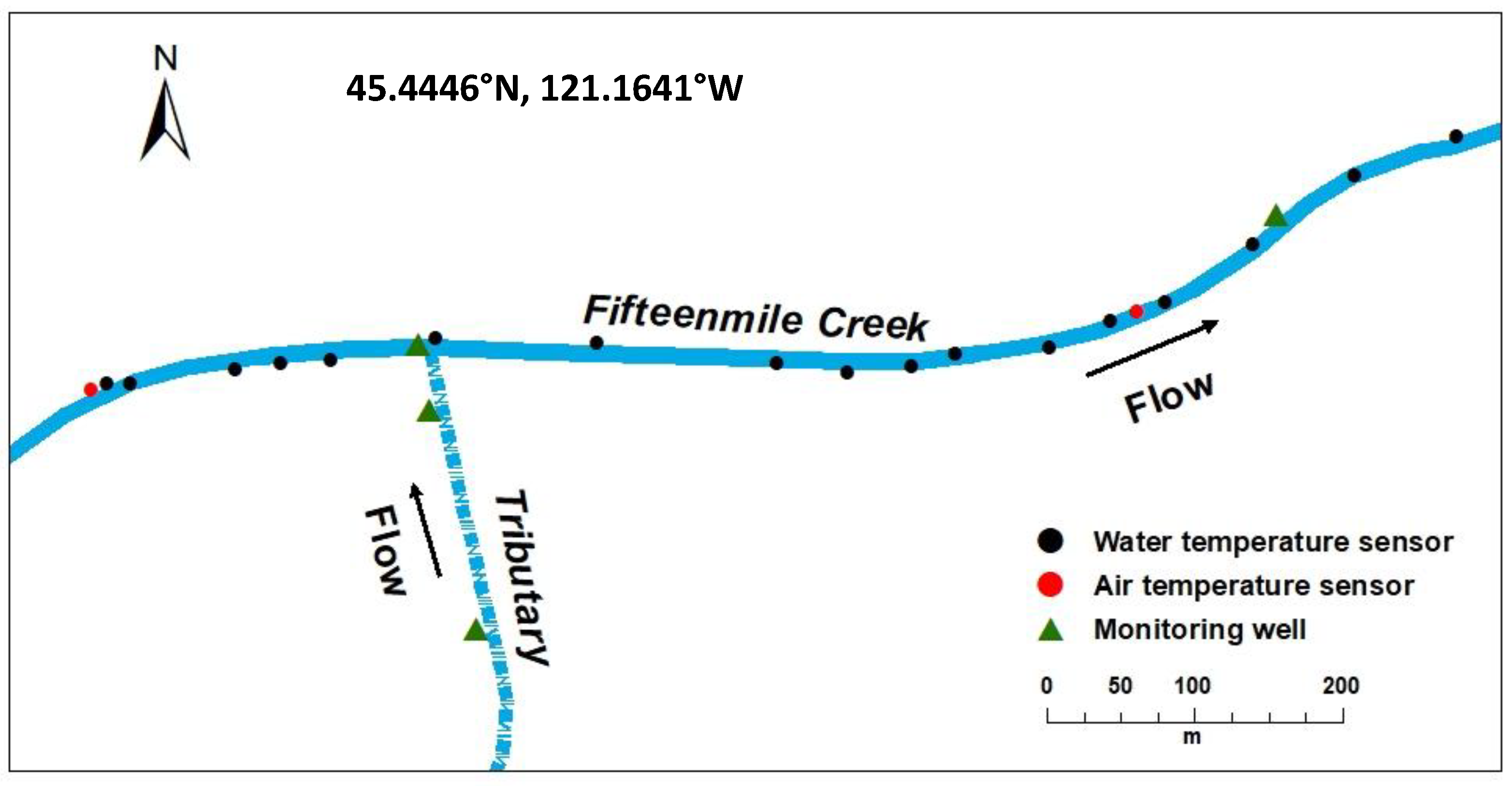
Four driven-point monitoring wells, each equipped with an automated water level and temperature logger (model U20, Onset Computer Corp., Bourne, MA, USA), were installed to measure water level and temperature at the 15-MC and on one intermittent tributary. The tributary has active surface streamflow during the early part of the snowmelt runoff season (January through early March), then in spring and summer is mainly subsurface flow. Two of the wells (SW-1 and SW-2) were installed in the 15-MC reach. Well SW-1 was located 6 m upstream of the confluence, and SW-2 was placed 500 m downstream of SW-1. The two other wells were located in the tributary at 20 m (TW-1) and 110 m (TW-2) upstream of the confluence with 15-MC (Figure 1). All the wells were pounded in the stream until they reached bedrock, typically at less than 1.5 m depth. The wells were made out of galvanized steel pipe (32 mm diameter) and have a 1.2 m length screen (60 gauge) section in the bottom.
A descriptive analysis approach including graphs, mean and maximum daily temperature, and Pearson’s correlation coefficient (r) between air and stream temperature was used. Based on the Shapiro–Wilk test results for normality, stream temperature and shallow groundwater temperature data were not normally distributed, and therefore non-parametric approaches were used. A Kruskal–Wallis one-way analysis of variance (ANOVA) test was conducted to assess daily averaged stream temperature variability at all stream temperature locations and between tributary and stream monitoring wells. The Tukey test was used to conduct pairwise comparisons of the wells. The Mann–Whitney U test was used to compare daily averaged subsurface temperature of the two wells in the tributary to daily averaged subsurface temperatures of the two wells along the valley reach. SigmaPlot® version 14.0 (Systat Software, Inc., San Jose, CA, USA) was used for the statistical analyses.
2.1.2. Stream Temperature and Environment Interactions—The 15-MC Valley Scale
Stream and air temperature data and streamflow, weather, and land cover information were used to parameterize an SVR model developed for assessing stream temperature variability and environment relationships along the 15-MC riparian corridor.
Stream and Air Temperature Relationships
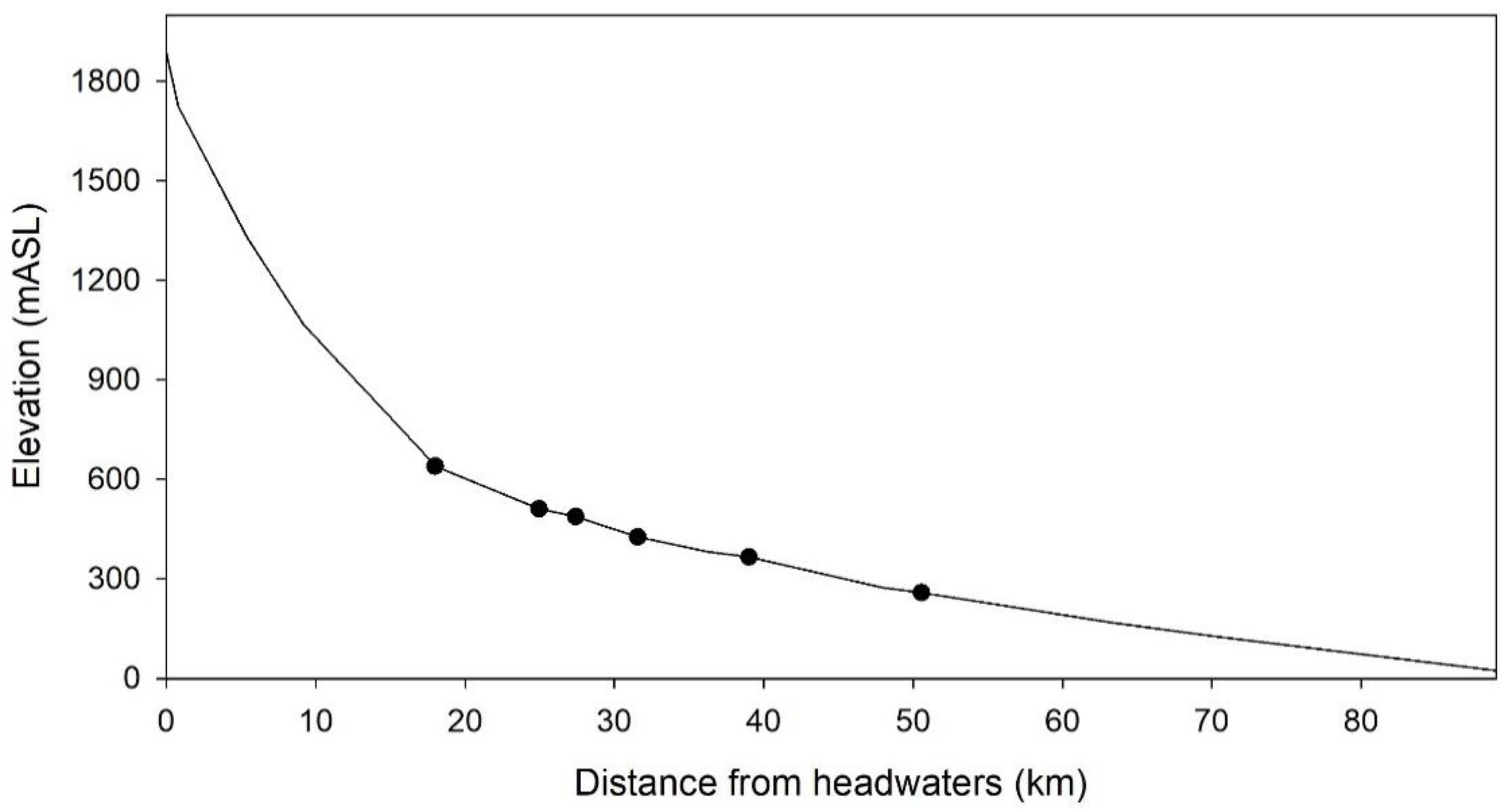
Temperature data were collected from seven different agriculture valley locations ranging between 260 and 640 mASL (Figure 2). In addition to four sites instrumented for measuring air and stream temperature, we used stream temperature data courtesy of the Oregon Department of Fish and Wildlife (ODFW) collected at three other locations. Air and temperature data were collected using Hobo Tidbit sensors (Onset Computer Corp., Bourne, MA, USA) sensors, while data from the ODFW monitoring sites were collected using Hobo Pro V2 sensors (Onset Computer Corp., Bourne, MA, USA). Both sensor models have an accuracy of ± 0.2 °C. Field-measured data were used for estimating daily averaged mean (mean), maximum (max), seven-day average (7DA), and the seven-day average of the daily maximum (7DADM).
Streamflow and Weather Information
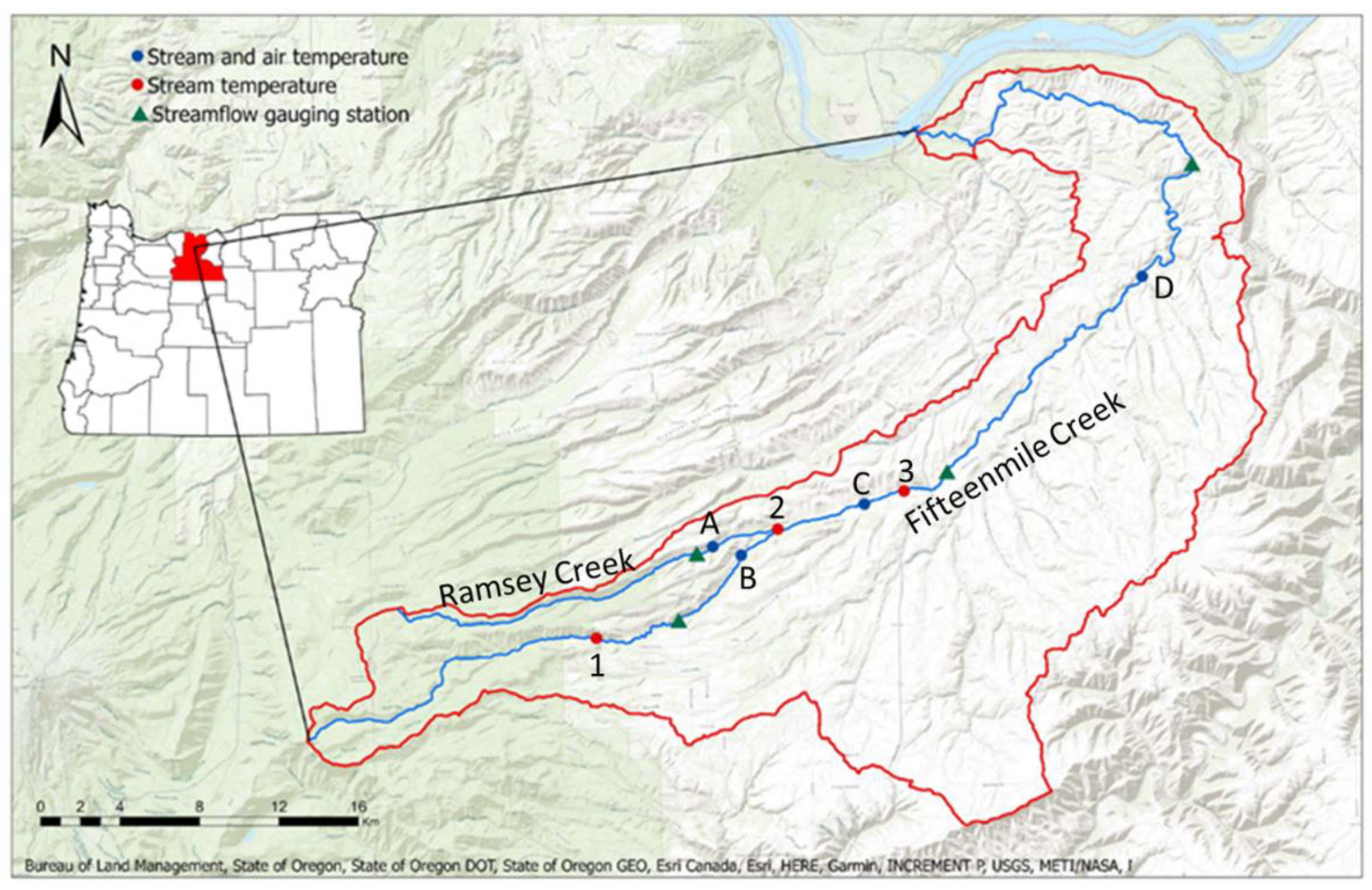
Streamflow data were obtained from four gauging stations managed by the Oregon Water Resources Department (OWRD) [71]. These stations are located along 15-MC, upstream of Ramsey Creek’s confluence, along Ramsey Creek, outside of Dufur, OR, and at a station located further downstream near Moody, OR (Figure 3).
Data regarding total daily precipitation, maximum, mean, and minimum air temperature, mean dew point temperature, and minimum, mean, and maximum vapor pressure deficit were obtained from Parameter-elevation Regressions on Independent Slopes Model (PRISM) datasets [72]. PRISM datasets use nearby monitoring station observations as inputs in a regression function to determine each grid cell’s value. Rasters containing the above environmental variables were downloaded from the PRISM website (https://prism.oregonstate.edu/, accessed on 1 March 2019), and the extract by points function in ArcGIS Pro (Version 2.5.1, Redlands, CA, USA) was used to extract the PRISM data for each sensor location.
Land Cover
Land cover was assessed using the United States Department of Agriculture National Agricultural Imagery Program (NAIP) data from 2016. The NAIP imagery was downloaded from the U.S. Geological Survey Earth Resources Observation and Science website (https://earthexplorer.usgs.gov/, accessed on 16 January 2020). The imagery used consists of red, green, blue, and near-infrared bands with a one-meter resolution.
The support vector machine (SVM) classification tool in ArcGIS Pro (Version 2.5.1, Redlands, CA, USA) was used to classify the NAIP imagery into several land cover categories (shrub/rangeland, open water, forested areas, and other vegetated areas). SVM is advantageous over classifiers such as the maximum likelihood classifier as it does not require samples to be normally distributed. The NAIP image was initially segmented using the Segmentation toolset, and polygons were drawn around representative samples of each class using the Training Sample Manager. After examining the initial results of classification and adding additional training samples as needed, an Esri Classification Definition (.ecd) file was created and used for the SVM classification of the NAIP image.
Assessment and confusion matrix tools in ArcGIS Pro were used on 511 data points to calculate user’s accuracy (an indication of type 1 error), producer’s accuracy (an indication of type 2 error), and the kappa coefficient. A stratified random approach was used to select the sampling points. Overall accuracy indicates the number of pixels correctly classified divided by the total number of pixels sampled. User’s accuracy represents whether pixels were accurately classified and is calculated based on the number of pixels correctly classified into a given class divided by the total number of pixels classified into the same class. The producer’s accuracy represents how well ground features were classified and is calculated by dividing the number of correctly classified pixels of a given class by the total number of reference pixels of a given class. The kappa coefficient indicates the agreement between predicted classes and actual classes, in which 0 indicates no agreement and a value of one indicates total agreement.
For land cover classification near each sensor’s location, a 30 m buffer was delineated on both sides of the stream for a distance of 100 and 1000 m upstream of each sensor. Percent cover was determined by dividing the number of pixels within the buffer classified as a given land cover type (e.g., forest, agriculture, rangeland, water) by the total number of pixels.
Support Vector Regression Model
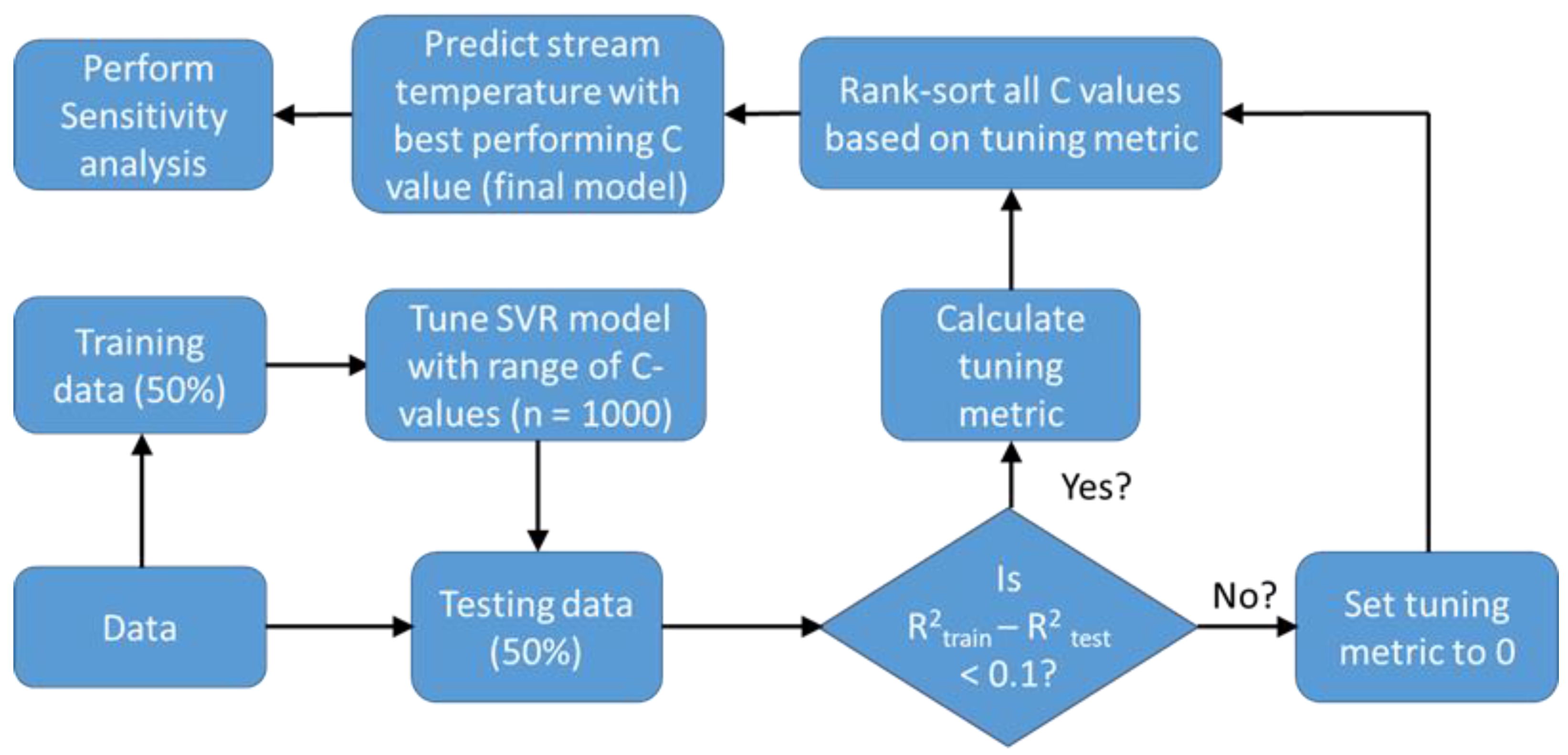
An SVR model was used to evaluate the relationship between stream temperature and thirteen different environmental variables (Table 1). A flowchart of the SVR process used in this study is provided in Figure 4. Stream and air temperature data collected on-site, streamflow information obtained from the OWRD website, and data obtained from PRISM datasets were used to parameterize the SVR model.
The SVR analysis included data from 1 July 2014 to 31 December 2016. After examining multiple environmental parameters, 13 variables (Table 1) were selected. Variables were also selected to reduce the similarity between individual parameters (e.g., forest cover at 30 m buffer vs. forest cover at 100 m).
Although SVR does not assume normality, many machine-learning models better characterize patterns when the variables are approximately normally distributed. All data were screened for normality by examining the skew of each variable. If the |skew| is ≤ 1, the variable is considered normally distributed [73]. All variables outside this range were positively skewed and were log-transformed. The log-transformed variables satisfied the skew criteria for most variables, except for PPT, which had a skew of 1.96. Although the skew was >1, the transformation significantly reduced the skew and was therefore retained for analysis. SVR is sensitive to variables that vary over different orders of magnitude. Therefore, all variables were Z score transformed, which scales the data such that all variables have a mean of 0 and a standard deviation of 1. The SVR model was programmed in Python using an algorithm developed by scikit learn (sklearn.svm.SVR; [74]). All default parameters were used, except the kernel and C. The linear kernel was used, which is advantageous because the linear kernel produces coefficient weights that are useful for evaluating each predictor variable’s importance. The regularization parameter C and values were randomly selected between 10−6 and 102.
The entire dataset was randomly split in half for training and testing cross-validation. The SVR model was tuned using the training dataset and was evaluated for overfitting using the testing dataset. During each iteration (n = 1000), a different C value was used to train the model, and the resulting model was used to predict the values of the testing dataset. Overfitting occurs when the model performance is high for the training dataset but substantially lower for the testing dataset. While no critical threshold exists to indicate the presence of overfitting, if the difference in the R2 between the training and testing model performance is >0.1, then overfitting was assumed to be present, and the tuning values were discarded. We developed a custom tuning metric for the remaining values to rank each randomly selected training and testing the dataset’s performance for each iteration. The C value associated with the best-performing model was retained for further analysis.
Using the best-performing C value, the final SVR model was developed as previously described. The dataset was randomly split in half for training and testing datasets to quantify overfitting. During each iteration (n = 1000), the training and testing performance and the coefficient weight of each variable were recorded. Additionally, the model was used to predict the stream temperature of the entire dataset. The overall fit of the model was evaluated by comparing the averaged predictions to the observed values.
Finally, a sensitivity analysis was performed. During each iteration of the final run, the model was used to predict a synthetic dataset where all predictor variables were held constant at their mean value (i.e., 0 given that each was Z score transformed) except for a single predictor variable that was allowed to vary ±2 standard deviations of its mean. By repeating this process for each predictor variable, we directly compared each predictor variable’s independent effect.
The SVR model was used to evaluate 16 different scenarios (Table 2). First, the model was run for each stream temperature category (mean, max, 7DA, and 7DADM) for the entire study’s entire duration using the 13 environmental variables outlined in Table 1. Next, the analysis was run for each stream temperature category using air temperature and streamflow (e.g., labeled as 7DADM_Q+A). Finally, we applied the SVR model based on seasonal streamflow characteristics, divided into the seasons with highest streamflow (October through May) and lowest streamflow (June through September), using five environmental variables which exhibit seasonal changes (i.e., mean air temperature, VPD, PPT, Q, and max–min air temp). We assessed each SVR analysis’s performance based on the coefficient of determination (R2) of observed versus modeled temperatures.
3. Results
3.1. Stream and Air Temperature Variability—The Reach Scale
3.1.1. Stream Temperature
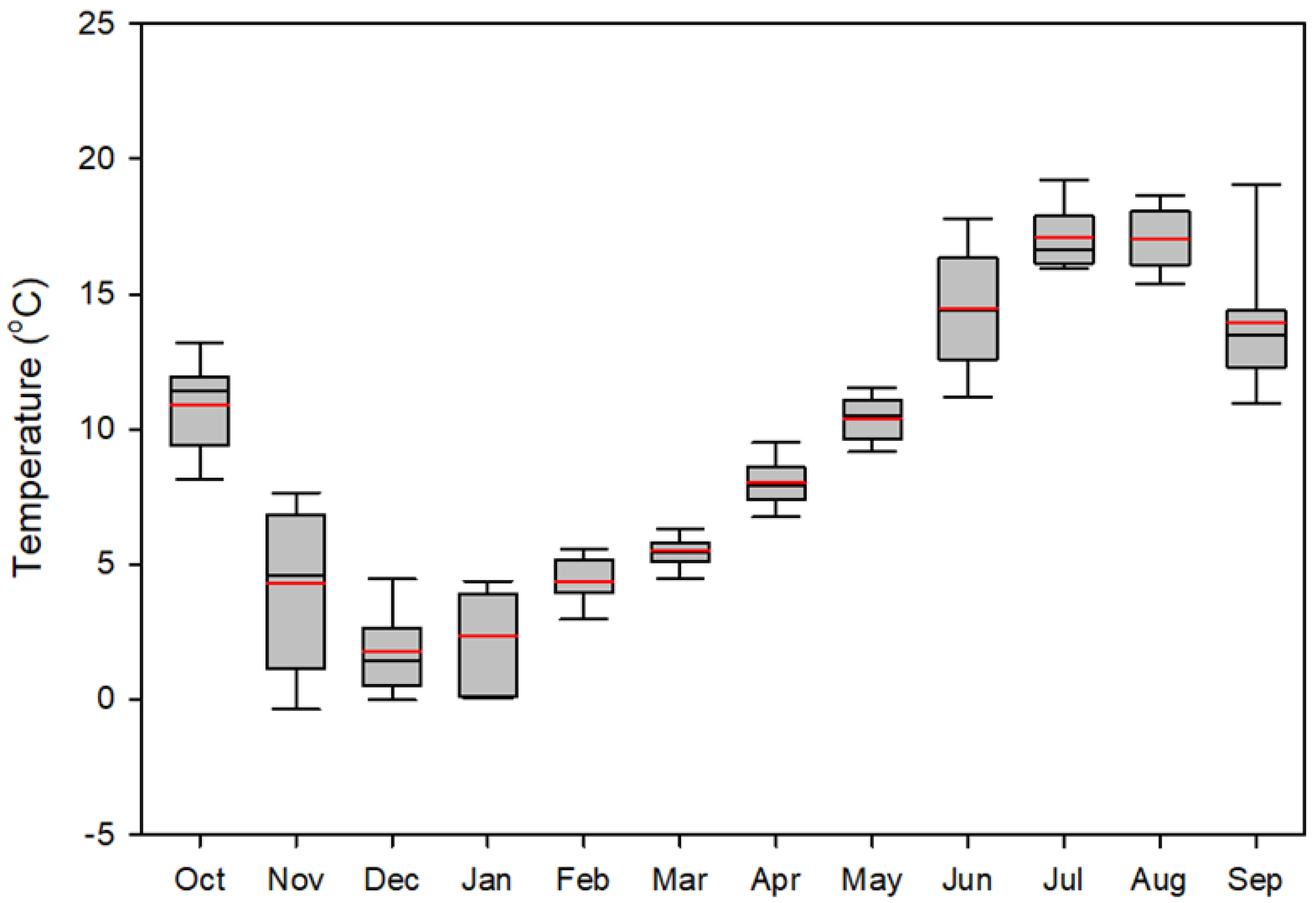
Based on the ANOVA, there were no statistical differences (p < 0.05), regardless of aspect or canopy cover, in 7DA, daily maximum, and mean temperature levels for all 17 sensor locations along the 800 m reach. Daily averaged stream temperature from August 2015 to July 2016 ranged from 0 to 21 °C, with a mean value of 9 °C ± 0.3. The lowest daily mean stream temperature occurred in December (2.9 °C) and the highest daily mean stream temperature in August (18 °C) (Figure 5).
3.1.2. Stream and Subsurface Flow Temperature
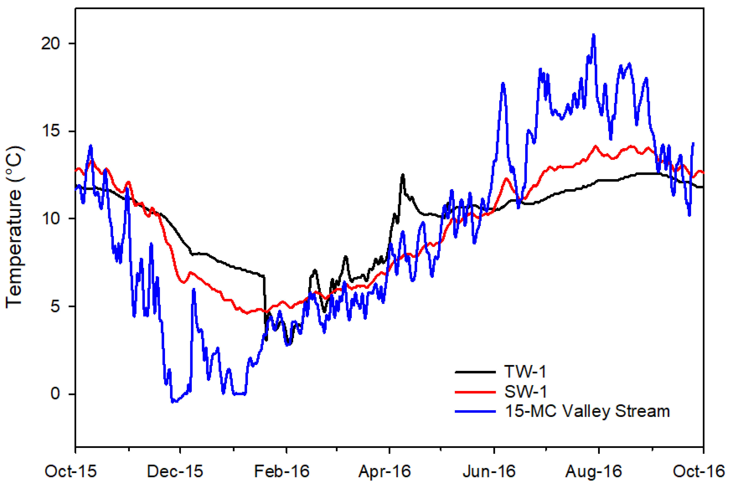
Daily averaged subsurface flow temperature levels in both the tributary and 15-MC were less variable than surface stream temperature, with subsurface flow temperatures generally being warmer than surface stream temperature during the winter and generally cooler than surface stream temperatures during the summer (Figure 6). Temperature differences of up to 8 °C in summer, and 10 °C in winter, between surface stream and tributary subsurface flow locations were observed.
Based on the Mann–Whitney U test, no significant difference (U = 66124.5, p > 0.05) between the daily averaged subsurface temperature of the two stream wells (median = 10.5 °C, mean = 9.9 °C ± 0.2) and the two tributary wells (median = 10.7 °C, mean = 9.8 °C ± 0.1) was observed. Greater maximum subsurface flow temperature levels were observed in the 15-MC wells than in the tributary ones. The two wells closest to the confluence (SW-1 and TW-1) exhibited lower mean stream temperature than the two (SW-2 and TW-2) farther away (Table 3).
Based on the ANOVA (p ≤ 0.001) and the Tukey test (p ≤ 0.05), results showed statistical differences in daily averaged temperature between all wells except for TW-2 vs. SW-1 and SW-1 vs. TW-1 (Table 4).
A seasonal trend in shallow groundwater temperature response was observed in all wells. One of the wells (TW-1) in the tributary showed the lowest temperature values in the summer and the most significant decrease in temperature during the snowmelt runoff season. We attributed this response to the location near the confluence with the main creek. The range of mean daily shallow groundwater temperatures was much less than that of the riparian air temperature.
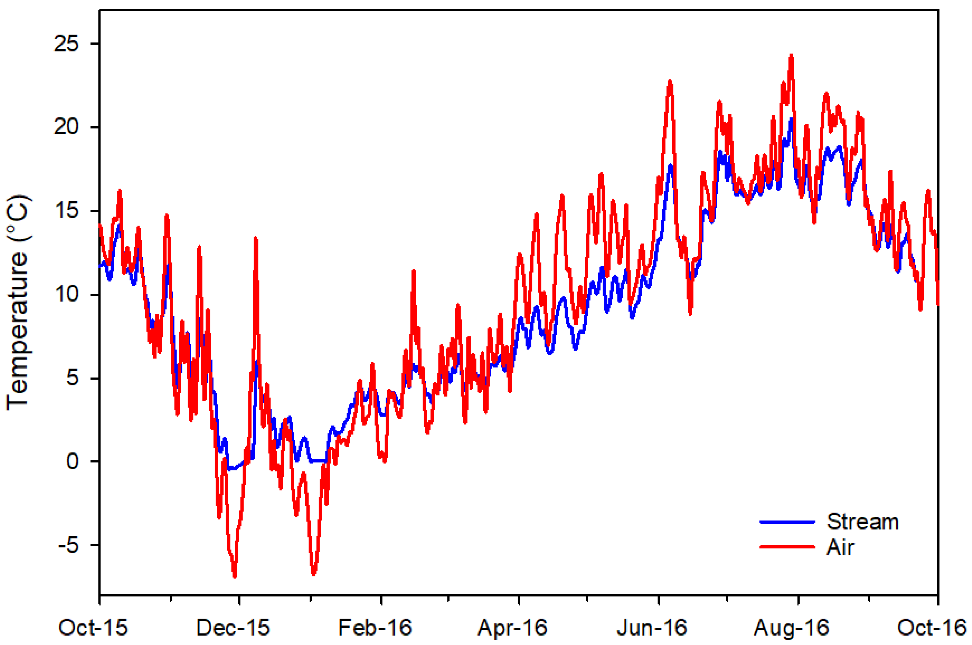
Stream temperature followed the general seasonal trend of air temperature. Daily averaged air temperature fluctuations were greater than stream temperature (Figure 7). Air temperature levels were significantly greater (up to 8 °C) than stream temperature during spring and summer. Peak maximum temperature for air (24 °C) and stream (17 °C) occurred in August 2015. Based on Pearson’s correlation, a strong correlation (r) = 0.97 between all-sensor mean air temperature (n = 2) and mean stream temperature (n = 17) was observed along the entire 800 m reach.
3.2. Valley Scale
3.2.1. Stream Temperature
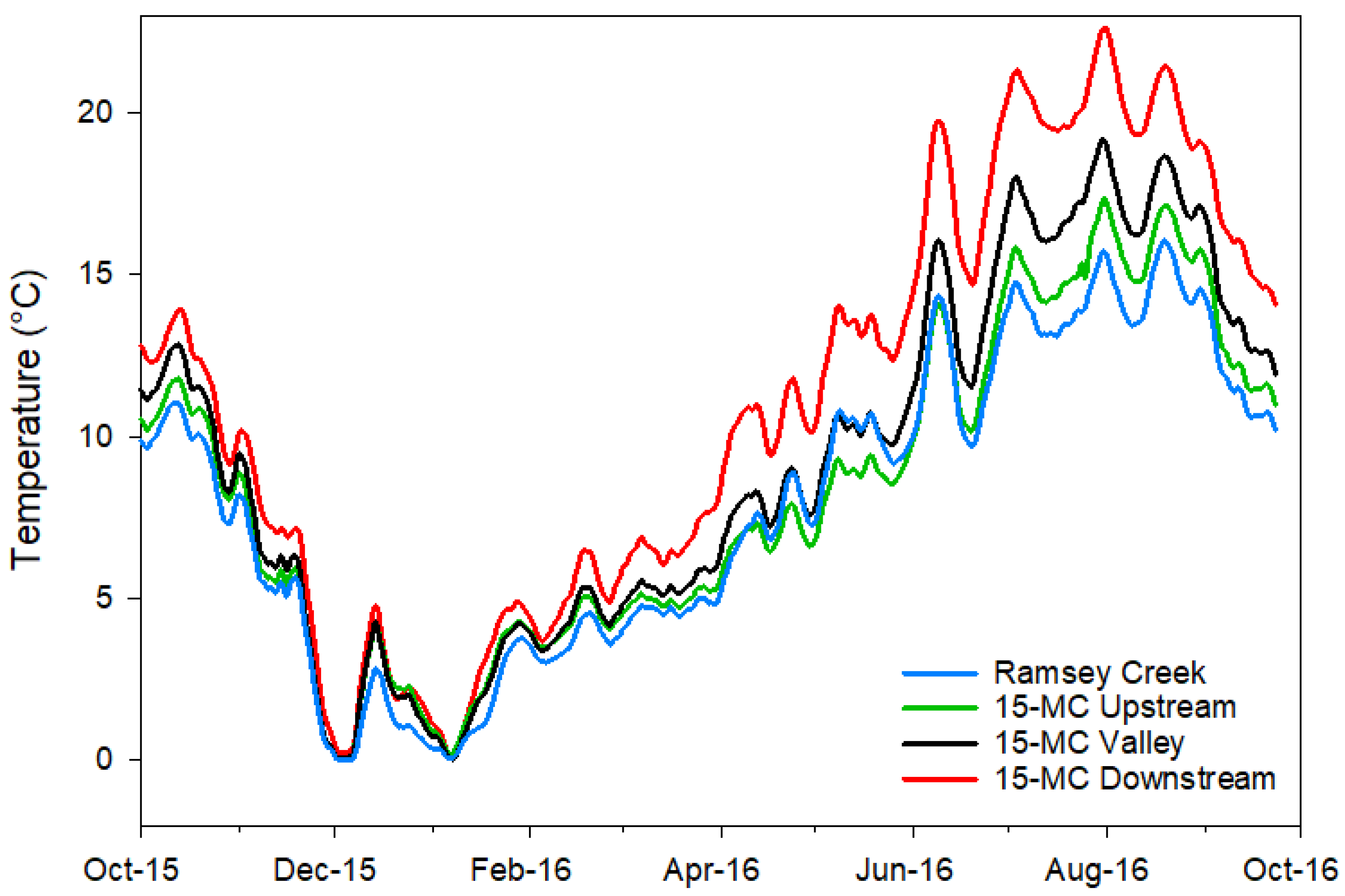
Greater stream temperature levels were observed in the lower-elevation sites (i.e., 15-MC valley and 15-MC downstream). Differences in temperature between study site locations were most significant during the summer months (Figure 8). A difference in the 7DA of up to 5 °C was observed between the highest-elevation site (Ramsey) and the 15-MC downstream site. Lower temperature variability among study sites was observed during late fall and winter.
Maximum and mean daily averaged stream temperature levels were highest at the downstream site location: 24.0 and 10.8 °C. The lowest maximum and mean daily stream temperatures were observed at the site located at the Ramsey tributary site (17 and 7.7 °C), which also experienced the slightest fluctuation in stream temperature during the year. The 7DA stream temperature in the downstream site exceeded the maximum threshold temperatures for salmonid and some other cold-water fish rearing (16 °C) and migration (18 °C) during the summer (Figure 8).
3.2.2. Streamflow
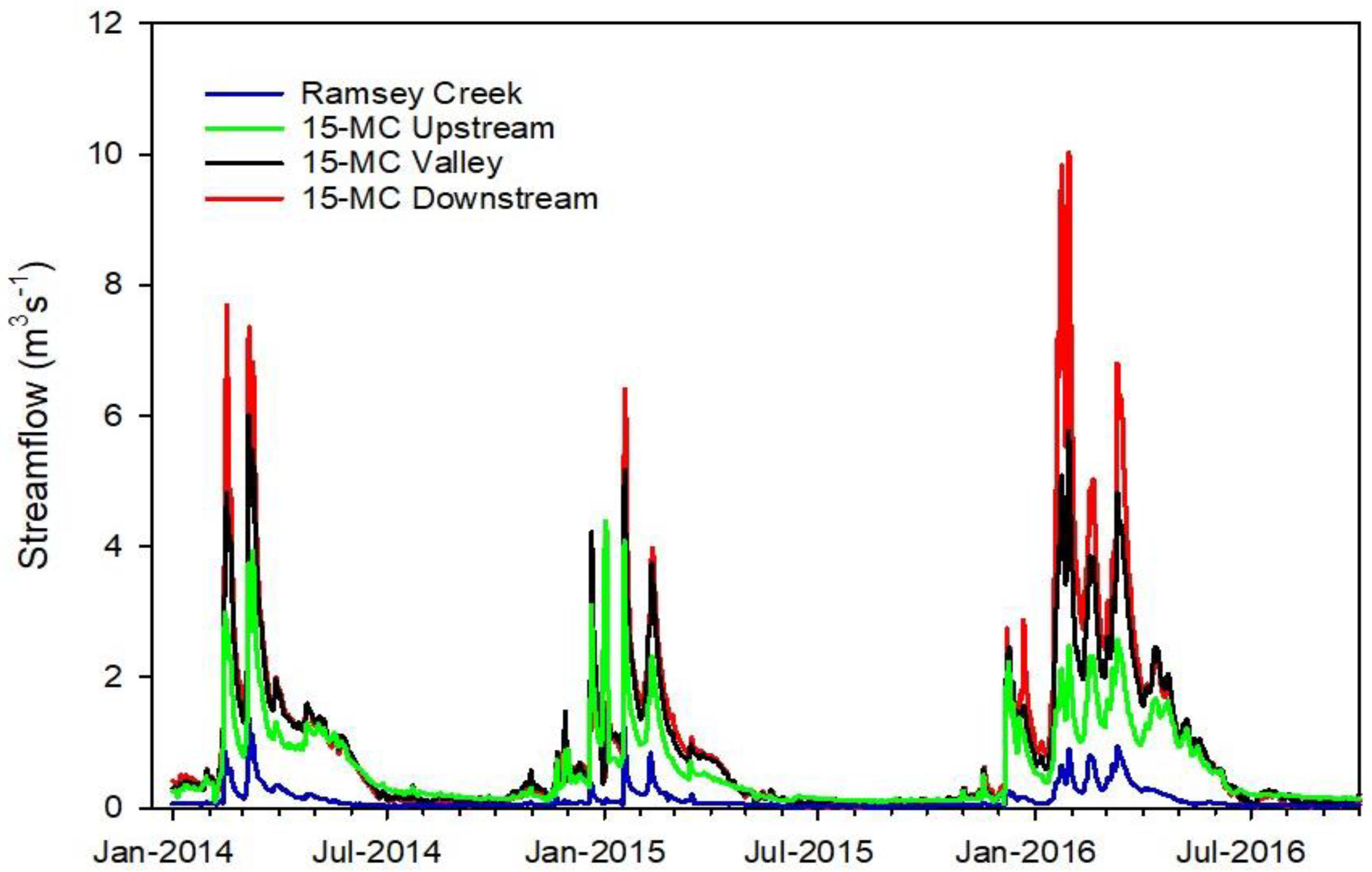
Streamflow was generally greater at the 15-MC downstream site and lowest at Ramsey Creek, with flow peaks corresponding to snowmelt periods in early spring for all sites. The lowest streamflow levels were reported during the summer, with the tributary Ramsey Creek at 0.2 m3 s−1 and 15-MC upstream at 0.7 m3 s−1. Larger streamflows were observed at the 15-MC downstream site in the spring of 2016 compared to the previous years. In contrast, lower streamflows in the spring season were observed at the 15-MC upstream site in 2016 than in 2014 and 2015 (Figure 9).
3.2.3. Riparian Land Cover Classification
For 15-MC and Ramsey Creek, most land cover (within 30 m on either side of the center of the stream channel) was classified as forested (46%) and shrubland (23%). The riparian areas upstream of Ramsey Creek and 15-MC’s confluence were largely forested (52%), with shrubland accounting for 14%. Approximately 10% of the riparian area upstream of the confluence was classified as herbaceous or planted fields. Downstream of the confluence, there is a slight reduction in forest cover. In the mid-section of 15-MC, between the confluence with 15-MC and Ramsey Creek and the downstream study site (Figure 3, Site D), forest cover accounts for 45% of riparian cover, and shrubland accounts for 31% of riparian cover. Herbaceous areas or planted fields accounted for approximately 9% of riparian land cover in the mid-section of 15-MC. Downstream of site D, approximately 38% of the riparian area is classified as forested, and 31% as shrubland. Approximately 10% of the riparian area between site D and the Columbia River’s confluence was classified as herbaceous or planted fields.
The overall accuracy of the SVM classification was 89%. Both the producer’s accuracy and the user’s accuracy ranged from 0.73 to 1, with mean values of 0.89 and 0.88. Cohen’s kappa was 0.88, indicating good agreement between predicted and actual class.
3.2.4. SVR Model
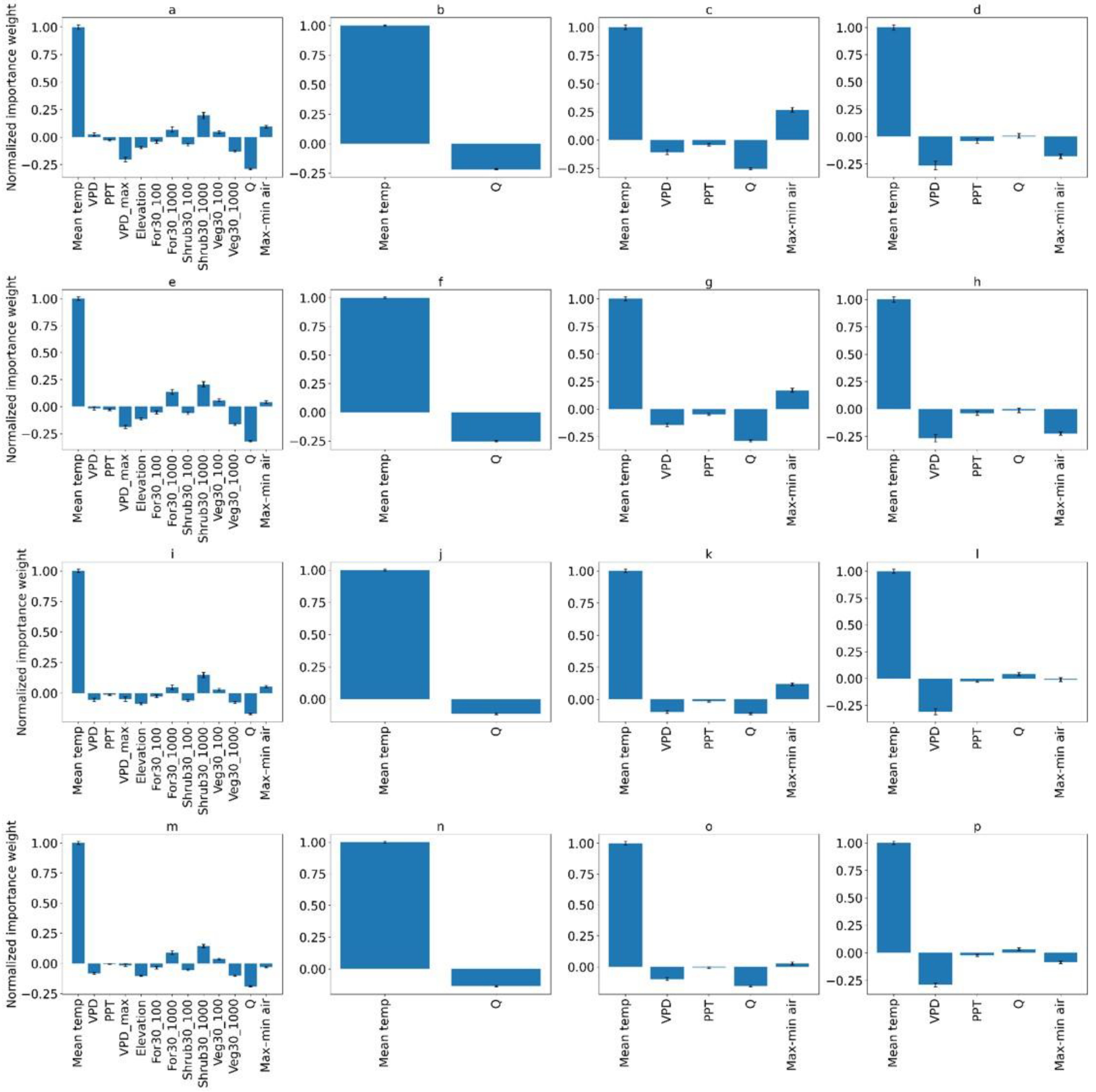
For each environmental variable tested in each scenario, each parameter’s mean importance was calculated and scaled from −1 to 1. A value of −1 or 1 indicated the greatest either negative or positive relationship, respectively. Values close to 0 indicate little to no relationship between the predictor and response variable. Mean temp (i.e., mean daily air temperature) has a strong positive relationship stream temperature and had the greatest scaled mean importance (Figure 10).
Increases in daily mean air temperature resulted in increases in predicted stream temperature for all the SVR model scenarios tested. With the exclusion of the scenarios that used only data from warmer months (e.g., 7DADM_Jun–Sept), increased flow (Q) generally resulted in decreased predicted stream temperature (weighted importance ranging from −0.32 to −0.11). Land cover was slightly associated with stream temperature changes and indicated conflicting patterns. A negligible impact of forested land cover (i.e., For30_100 and For30_1000) on stream temperature was found. Similarly, shrub cover (i.e., Shrub30_100 and Shrub30_1000) were minimally associated with stream temperature. The mean VPD was negatively related with stream temperature for 7DADM_Jun–Sept, max_Jun–Sept, 7DA_Jun–Sept, and mean_Jun–Sept scenarios (relative mean importance of −0.27 to −0.31) (Figure 10).
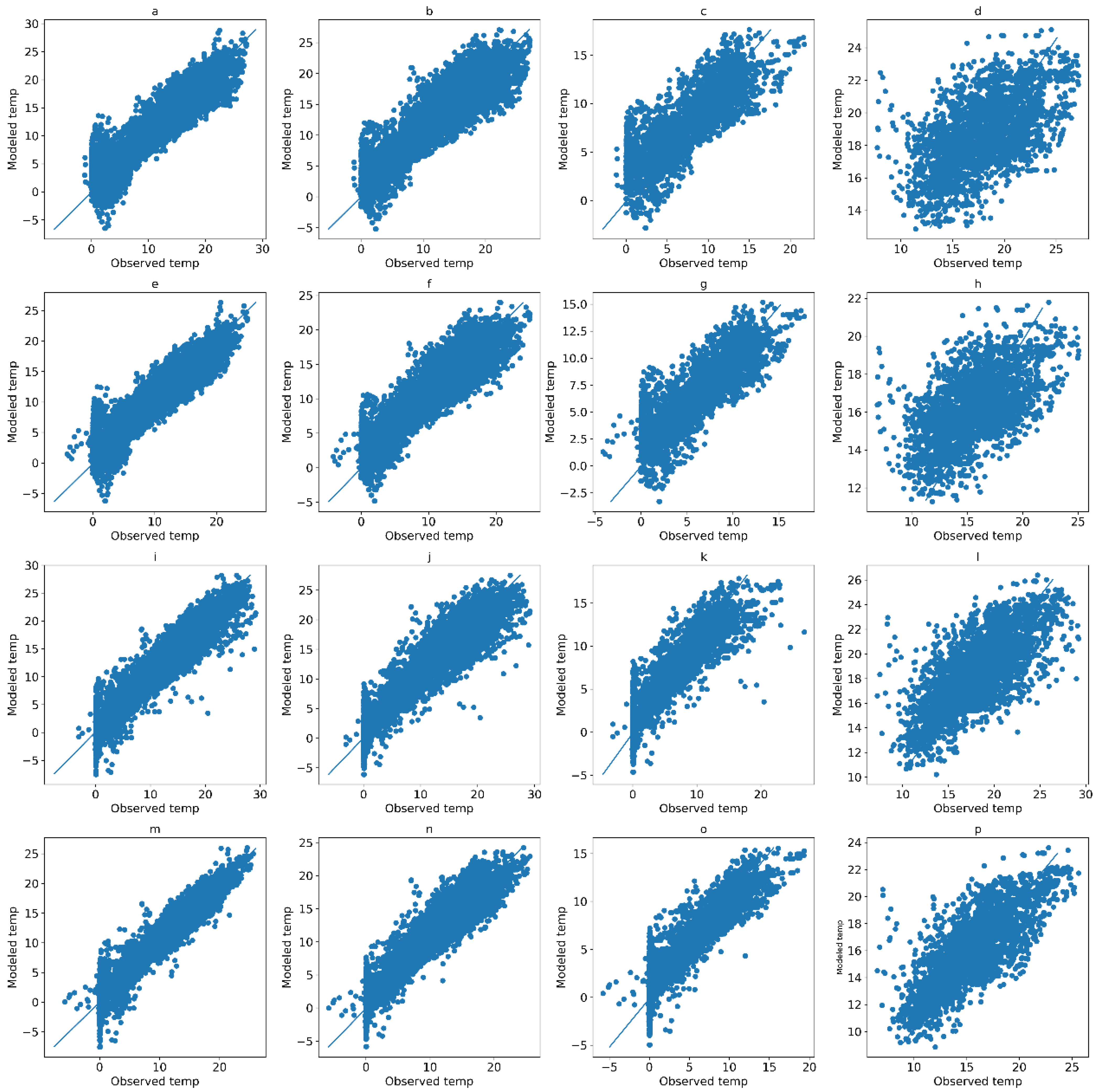
The scenarios (i.e., 7DADM, max, 7DA, and mean) that incorporated all 13 environmental variables and that included data across all seasons generally performed better than the rest (Figure 11). For these scenarios, R2 ranged from 0.86 to 0.92 (mean of 0.89). The R2 across all scenarios ranged from 0.36 to 0.92, with an average R2 of 0.75 (Table 5). R2 ranged from 0.83 to 0.89 (mean of 0.86) for analyses that used only Q and mean daily air temperature (e.g., 7DADM_Q+A). Additionally, mean and max scenarios performed somewhat better than 7DA and 7DADM. Of all scenarios, those using only data from June through September (e.g., 7DADM_Jun–Sept) performed the worst (mean R2 of 0.48).
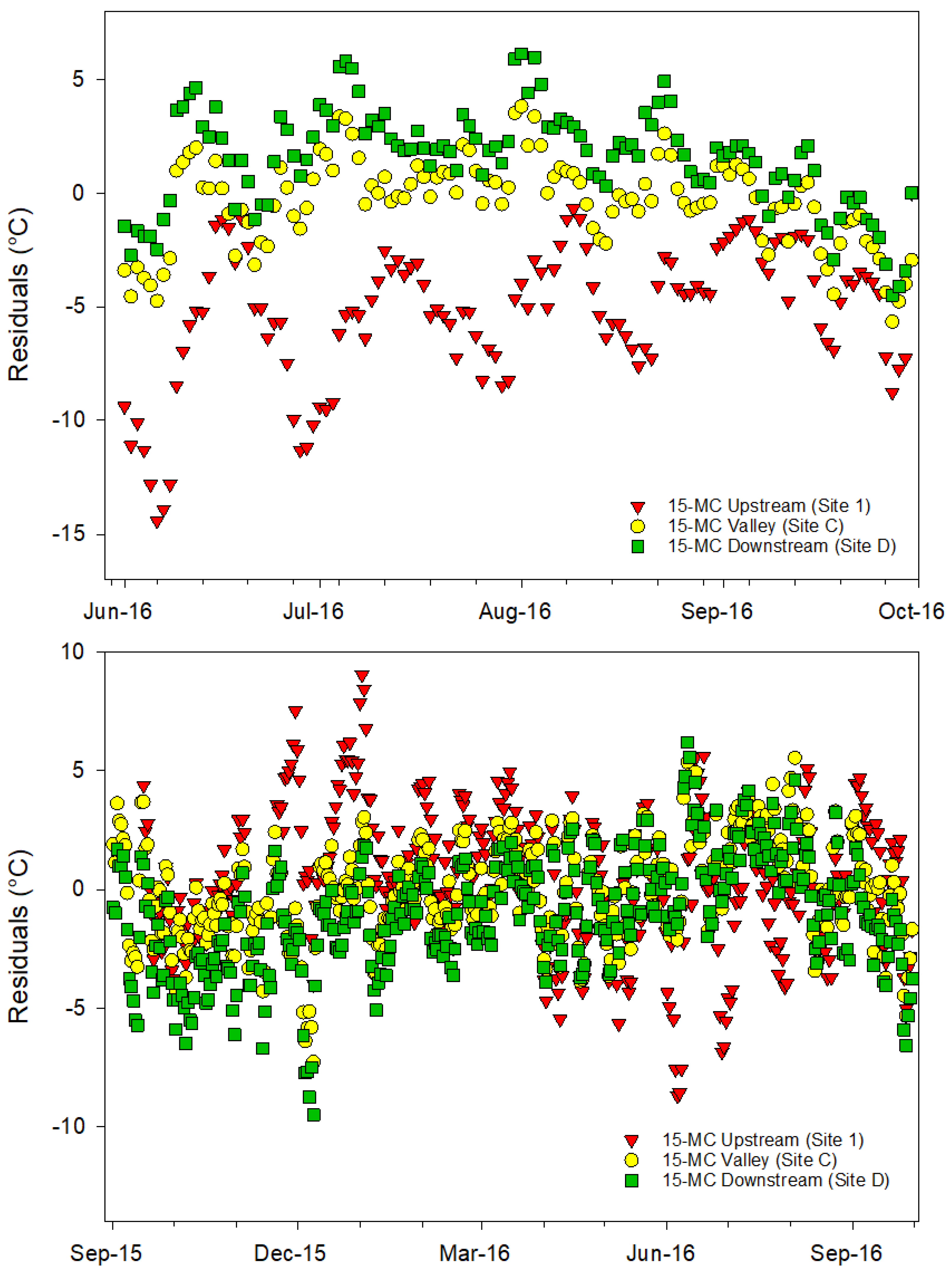
In general, the SVR model did not predict extreme maximum and minimum stream temperatures (Figure 11 and Figure 12). This was most pronounced when the model was run using only seasonal data, particularly for scenarios using summer data (e.g., 7DADM_Jun–Sept). Trends were also indicated in the residuals (observed value-predicted value) for these scenarios. The model tended to overpredict temperatures at sites furthest upstream and, to a lesser degree, underpredict temperatures at sites further downstream during the summer months. A sinusoidal trend is also indicated for the residuals of many of the sensors for these summer month scenarios (Figure 12, top).
The sensitivity analysis results (data not shown) indicated the same trends as the scaled mean importance of each variable, with changes in air temperature being the strongest predictor of stream temperature for all scenarios. An increase of one standard deviation in air temperature (8.2 °C) was associated with a 5.6, 5.8, 6.1, and 5.2 °C increase in stream temperature for 7DADM, mean, max, and 7DA scenarios, respectively. For Jun–Sept scenarios, an increase of one standard deviation in air temperature (3.5 °C) was associated with a stream temperature increase between 2.7 and 3.6 °C. In contrast, an increase of one standard deviation in streamflow resulted in a decrease in stream temperature of 1.6 and 0.8 °C for 7DADM and 7DADM_Oct–May scenarios, respectively.
4. Discussion
This research examined the relationship between stream temperature and various environmental parameters in a semiarid riparian ecosystem. Study results show that air temperature, followed by Q in the cooler months and VPD during the warmer months, was the most significant factor associated with stream temperature at both the reach and valley scales. Similar to other studies [28,75,76], we found that stream temperature and environment relationships are highly seasonal. Q was negatively related with stream temperature and was the second-largest factor influencing stream temperature. The exception to this was when Q was lowest, in which there was a minimal positive association indicated between streamflow volume and stream temperature. By comparison, Isaak et al. [7] found that streamflow explained almost half of stream temperature variation during summer months while air temperature accounted for most long-term stream temperature differences for 18 monitoring sites in the northwestern United States.
We found no statistical differences in stream temperature between sites with different canopy cover. Land cover was marginally associated with stream temperature. Similarly, Łaszewski and Kiryła (2008) used Sentinel (1 and 2) imagery to assess the relationship between forested areas and stream temperature and did not find statistically significant differences in thermal regimes based on forest cover [77]. This contrasts with Horne and Hubbart [78], who found that forested land use was negatively correlated with stream temperature at a West Virginia study site. Other studies have also found riparian vegetation shading to be negatively correlated with stream temperature (e.g., [42,79,80,81]).
Due to the frequency of NAIP imagery collection, riparian land cover was only assessed for the summer of 2016. Land cover classes may have changed throughout this study (e.g., agricultural fields may have been harvested). However, since most of the riparian areas in the valley are under a long-term conservation program agreement, it was assumed that minimal land cover changes occurred along the entire 15-MC riparian corridor evaluated. While the NAIP-based classification approach yielded generally good results, this approach may not have accounted for shading associated with other vegetation, including understory. Further, while riparian land cover and stream shading are related, riparian vegetation classification should not be directly equated with riparian shading. Other factors, such as slope and aspect, can also influence incoming solar radiation and were not assessed during this study. The aggregated effect of vegetation along the entire stream may help to modulate stream temperature overall. For example, a study conducted by the Oregon Department of Environmental Quality using the Heat Source model [46] found that increasing riparian vegetation to site potential and increasing Q would reduce peak 7DADM, with increased riparian vegetation being the most important factor influencing stream temperature [82].
The marginal temperature differences between different locations along the reach (regardless of canopy cover) may also be influenced by stream velocity and discharge. Steep gradients help move water through the landscape relatively rapidly during the snowmelt runoff season. As a result, movement through shaded or non-shaded areas may be less influential than at lower velocities. During the year, the lowest shallow groundwater temperatures were associated with greater rates of streamflow during the spring snowmelt but not the lowest annual stream temperatures, reemphasizing the importance of ambient conditions.
There was a lack of data regarding subsurface flows outside the 800 m reach evaluated; therefore, shallow groundwater flows were not included in the SVR analyses. Similar to that reported by Simmons et al. [80], our study indicated that colder groundwater inputs could influence stream temperature, at least at a small scale. This suggests that subsurface flows may serve as a modulating influence and potentially produce cold-water habitat at the confluence. Mean daily shallow groundwater temperatures just before the confluence with the intermittent tributary were lower than those downstream, indicating that the influence of groundwater inflows may be localized.
The overall SVR model performance varied with the stream temperature scenario tested, the environmental parameters included, and the period assessed (seasonal vs. full-year). Variations were expected based simply on the number of parameters used, as an increase in regression parameters is generally associated with an increase in R2 values. However, the inclusion of land cover parameters and additional atmospheric variables (e.g., PPT and VPD) modestly improved performance over the analysis that only used air temperature and Q. The SVR model performed the worst during the seasons when Q was the lowest and stream temperatures were the greatest. This suggests that other factors not examined in the SVR used in this study may also affect stream temperature.
The SVR model results highlight several limitations to the use of regression approaches. For example, hysteresis associated with seasonal changes is difficult to capture in stream temperature models. Regression models are often more effective for stream temperature modeling at weekly or longer scales due to the presence of autocorrelation at shorter time scales [22,83]. However, we found that the SVR model we tested generally performed better on daily scales than on weekly scenarios. Further, the relationship between air and stream temperature is not linear in all cases [22,84], particularly at high and sub-zero water temperatures. Therefore, non-linear approaches (e.g., [85]) are also commonly used. The SVR analysis applied in our study was able to predict general stream temperature patterns but did not predict extreme maximum and minimum stream temperatures (as the water temperature remains relatively constant with air temperature at or below freezing). This suggests that a non-linear approach may be more appropriate for modeling temperature beyond certain thresholds (e.g., sub-zero stream temperature). However, this study’s SVR approach is an easily replicable approach that can be applied at other study sites, provided that these limitations are acknowledged.
This research highlighted several critical areas for future research into stream temperature dynamics in semiarid systems. Stream temperature can be impacted by environmental characteristics that were beyond the scope of this study (e.g., riparian soil types). For example, streambed heat exchange can impact stream temperature dynamics of shallow streams [86]. Irrigation can also influence groundwater discharge to stream resulting in impacts on stream temperature [87]. Further, the monitoring sites selected for this study were chosen to represent different areas along the longitudinal gradient and were also based on landowner participation; additional sites at higher and lower elevations could provide a more comprehensive model. Land use and land cover beyond the riparian area may also play a role in stream temperature dynamics. While beyond this study’s scope, future research should address the role that ecohydrologic connections across the landscape (e.g., land-use practices outside of the riparian area) may play in stream temperature dynamics.
We did not attempt to model stream temperature regimes under alternative environmental conditions, such as altered land cover or increased air temperatures. Therefore, our results should be interpreted with caution regarding how changes derived from land management practices, such as the planting or removal of riparian vegetation, may influence stream temperature.
Author Contributions
N.D. and C.G.O. developed the study design and conducted field data collection. N.D., C.G.O. and G.J. contributed to data analyses and the writing of the manuscript. All authors have read and agreed to the published version of the manuscript.
Funding
This study was funded in part by USDA NIFA, the Oregon Beef Council (OBC 2015 and OBC 2016), and the Oregon Agricultural Experiment Station.
Data Availability Statement
Most of the data presented in this study are available in the article, the links within the article, or in the supplementary material. Additional information is available upon request.
Acknowledgments
The authors gratefully acknowledge the support from the various landowners in the area who provided access for sensor installation and field data collection. Also, we want to thank the Oregon Cattlemen Association and the Oregon Beef Council for their support of this research. Additionally, thanks go to the various graduate and undergraduate students from Oregon State University who helped with field activities related to the results here presented.
Conflicts of Interest
The authors declare no conflict of interest.
Appendix A

Table A1.
Distance from the beginning of the reach, aspect, and riparian vegetation cover above each stream temperature sensor.
Table A1.
Distance from the beginning of the reach, aspect, and riparian vegetation cover above each stream temperature sensor.
| Sensor# | Distance (m) | Aspect | Cover (%) |
|---|---|---|---|
| - | 0 | - | - |
| 1 | 15 | South | 4 |
| 2 | 24 | South | 95 |
| 3 | 80 | South | 11 |
| 4 | 98 | North | 84 |
| 5 | 121 | South | 68 |
| 6 | 171 | North | 74 |
| 7 | 252 | South | 76 |
| 8 | 344 | North | 79 |
| 9 | 371 | North | 66 |
| 10 | 401 | South | 75 |
| 11 | 425 | South | 70 |
| 12 | 470 | North | 92 |
| 13 | 503 | North | 78 |
| 14 | 534 | North | 79 |
| 15 | 596 | South | 90 |
| 16 | 660 | North | 92 |
| 17 | 725 | South | 56 |
| - | 800 | - | - |
References
- Demaria, E.M.C.; Roundy, J.K.; Wi, S.; Palmer, R.N. The Effects of climate change on seasonal snowpack and the hydrology of the northeastern and upper Midwest United States. J. Clim. 2016, 29, 6527–6541. [Google Scholar] [CrossRef] [Green Version]
- Godsey, S.E.; Kirchner, J.W.; Tague, C.L. Effects of changes in winter snowpacks on summer low flows: Case studies in the Sierra Nevada, California, USA. Hydrol. Process. 2014, 28, 5048–5064. [Google Scholar] [CrossRef]
- Ficklin, D.L.; Stewart, I.T.; Maurer, E.P. Effects of climate change on stream temperature, dissolved oxygen, and sediment concentration in the Sierra Nevada in California. Water Resour. Res. 2013, 49, 2765–2782. [Google Scholar] [CrossRef]
- Cline, T.J.; Schindler, D.E.; Walsworth, T.E.; French, D.W.; Lisi, P.J. Low snowpack reduces thermal response diversity among streams across a landscape. Limnol. Oceanogr. Lett. 2020, 5, 254–263. [Google Scholar] [CrossRef] [Green Version]
- Wang, L.; Lyons, J.; Kanehl, P. Impacts of urban land cover on trout streams in Wisconsin and Minnesota. Trans. Am. Fish. Soc. 2003, 132, 825–839. [Google Scholar] [CrossRef]
- Malcolm, I.A.; Soulsby, C.; Hannah, D.M.; Bacon, P.J.; Youngson, A.F.; Tetzlaff, D. The influence of riparian woodland on stream temperatures: Implications for the performance of juvenile Salmonids. Hydrol. Process. 2008, 22, 968–979. [Google Scholar] [CrossRef]
- Isaak, D.J.; Wollrab, S.; Horan, D.; Chandler, G. Climate change effects on stream and river temperatures across the northwest U.S. from 1980–2009 and implications for Salmonid fishes. Clim. Change 2012, 113, 499–524. [Google Scholar] [CrossRef] [Green Version]
- Kaushal, S.S.; Likens, G.E.; Jaworski, N.A.; Pace, M.L.; Sides, A.M.; Seekell, D.; Belt, K.T.; Secor, D.H.; Wingate, R.L. Rising stream and river temperatures in the United States. Front. Ecol. Environ. 2010, 8, 461–466. [Google Scholar] [CrossRef]
- Moatar, F.; Gailhard, J. Water temperature behaviour in the river Loire since 1976 and 1881. Comptes Rendus Geosci. 2006, 338, 319–328. [Google Scholar] [CrossRef]
- Webb, B.W.; Nobilis, F. Long-term changes in river temperature and the influence of climatic and hydrological factors. Hydrol. Sci. J. 2007, 52, 74–85. [Google Scholar] [CrossRef]
- Hari, R.E.; Livingstone, D.M.; Siber, R.; Burkhardt-Holm, P.; Güttinger, H. Consequences of climatic change for water temperature and Brown trout populations in alpine rivers and streams. Glob. Change Biol. 2006, 12, 10–26. [Google Scholar] [CrossRef]
- Webb, B.W.; Hannah, D.M.; Moore, R.D.; Brown, L.E.; Nobilis, F. Recent advances in stream and river temperature Research. Hydrol. Process. 2008, 22, 902–918. [Google Scholar] [CrossRef]
- Rasmussen, J.J.; Baatrup-Pedersen, A.; Riis, T.; Friberg, N. Stream ecosystem properties and processes along a temperature gradient. Aquat. Ecol. 2011, 45, 231–242. [Google Scholar] [CrossRef] [Green Version]
- Boyd, M.; Sturdevant, D. Scientific Basis for Oregon’s Stream Temperature Standard: Common Questions and Straight Answers; Oregon Department of Environmental Quality: Portland, OR, USA, 1997; pp. 1–29.
- Richter, A.; Kolmes, S.A. Maximum temperature limits for Chinook, Coho, and Chum salmon, and Steelhead trout in the Pacific Northwest. Rev. Fish. Sci. 2005, 13, 23–49. [Google Scholar] [CrossRef]
- Du, X.; Goss, G.; Faramarzi, M. Impacts of hydrological processes on stream temperature in a cold region watershed based on the SWAT equilibrium temperature model. Water 2020, 12, 1112. [Google Scholar] [CrossRef] [Green Version]
- Isaak, D.J.; Hubert, W.A. A hypothesis about factors that affect maximum summer stream temperatures across montane landscapes. JAWRA J. Am. Water Resour. Assoc. 2001, 37, 351–366. [Google Scholar] [CrossRef]
- Woltemade, C.J.; Hawkins, T.W. Stream temperature impacts because of changes in air temperature, land cover and stream discharge: Navarro river watershed, California, USA. River Res. Appl. 2016, 32, 2020–2031. [Google Scholar] [CrossRef]
- Johnson, S.L. Factors influencing stream temperatures in small streams: Substrate effects and a shading experiment. Can. J. Fish. Aquat. Sci. 2004, 61, 913–923. [Google Scholar] [CrossRef]
- Moore, R.D.; Nelitz, M.; Parkinson, E. Empirical modelling of maximum weekly average stream temperature in British Columbia, Canada, to support assessment of fish habitat suitability. Can. Water Resour. J. 2013, 38, 135–147. [Google Scholar] [CrossRef]
- Ebersole, J.L.; Wiginton, P.J.; Leibowitz, S.G.; Van Sickle, J. Predicting the occurrence of cold-water patches at intermittent and ephemeral tributary confluences with warm rivers. Freshw. Sci. 2014, 34, 111–124. [Google Scholar] [CrossRef]
- Caissie, D. The thermal regime of rivers: A review. Freshw. Biol. 2006, 51, 1389–1406. [Google Scholar] [CrossRef]
- Mayer, T.D. Controls of summer stream temperature in the Pacific Northwest. J. Hydrol. 2012, 475, 323–335. [Google Scholar] [CrossRef]
- Janisch, J.E.; Wondzell, S.M.; Ehinger, W.J. Headwater stream temperature: Interpreting response after logging, with and without riparian buffers, Washington, USA. For. Ecol. Manag. 2012, 270, 302–313. [Google Scholar] [CrossRef]
- Poole, G.C.; Berman, C.H. An ecological Perspective on in-stream temperature: Natural heat dynamics and mechanisms of heat-caused thermal degredation. Environ. Manag. 2001, 27, 787–802. [Google Scholar] [CrossRef]
- Daraio, J.A.; Bales, J.D. Effects of land use and climate change on stream temperature I: Daily flow and stream temperature projections. J. Am. Water Resour. Assoc. 2014, 50, 1155–1176. [Google Scholar] [CrossRef]
- Webb, B.W.; Clack, P.D.; Walling, D.E. Water–air temperature relationships in a Devon river system and the role of flow. Hydrol. Process. 2003, 17, 3069–3084. [Google Scholar] [CrossRef]
- Leach, J.A.; Olson, D.H.; Anderson, P.D.; Eskelson, B.N.I. Spatial and seasonal variability of forested headwater stream temperatures in western Oregon, USA. Aquat. Sci. 2017, 79, 291–307. [Google Scholar] [CrossRef]
- Van Vliet, M.T.H.; Ludwig, F.; Zwolsman, J.J.G.; Weedon, G.P.; Kabat, P. Global river temperatures and sensitivity to atmospheric warming and changes in river flow. Water Resour. Res. 2011, 47, W02544. [Google Scholar] [CrossRef]
- Lisi, P.J.; Schindler, D.E.; Cline, T.J.; Scheuerell, M.D.; Walsh, P.B. Watershed geomorphology and snowmelt control stream thermal sensitivity to air temperature. Geophys. Res. Lett. 2015, 42, 3380–3388. [Google Scholar] [CrossRef]
- Woltemade, C.J. Stream temperature spatial variability reflects geomorphology, hydrology, and microclimate: Navarro river watershed, California. Prof. Geogr. 2017, 69, 177–190. [Google Scholar] [CrossRef]
- Kelleher, C.; Wagener, T.; Gooseff, M.; McGlynn, B.; McGuire, K.; Marshall, L. Investigating controls on the thermal sensitivity of Pennsylvania streams. Hydrol. Process. 2012, 26, 771–785. [Google Scholar] [CrossRef]
- Tague, C.; Farrell, M.; Grant, G.; Lewis, S.; Rey, S. Hydrogeologic controls on summer stream temperatures in the McKenzie river basin, Oregon. Hydrol. Process. 2007, 21, 3288–3300. [Google Scholar] [CrossRef]
- Rutherford, J.C.; Blackett, S.; Blackett, C.; Saito, L.; Davies-Colley, R.J. Predicting the effects of shade on water temperature in small streams. N. Z. J. Mar. Freshw. Res. 1997, 31, 707–721. [Google Scholar] [CrossRef]
- Wondzell, S.M.; Diabat, M.; Haggerty, R. What matters most: Are future stream temperatures more sensitive to changing air temperatures, discharge, or riparian vegetation? JAWRA J. Am. Water Resour. Assoc. 2019, 55, 116–132. [Google Scholar] [CrossRef] [Green Version]
- Beschta, R.L. Riparian shade and stream temperature: An alternative perspective. Rangelands 1997, 19, 25–28. [Google Scholar]
- Cole, E.; Newton, M. Influence of streamside buffers on stream temperature response following clear-cut harvesting in western Oregon. Can. J. For. Res. 2013, 43, 993–1005. [Google Scholar] [CrossRef]
- Cross, B.K.; Bozek, M.A.; Mitro, M.G. Influences of riparian vegetation on Trout stream temperatures in central Wisconsin. North Am. J. Fish. Manag. 2013, 33, 682–692. [Google Scholar] [CrossRef]
- Studinski, J.; Hartman, K.; Niles, J.; Keyser, P. The effects of riparian forest disturbance on stream temperature, sedimentation, and morphology. Hydrobiologia 2012, 686, 107–117. [Google Scholar] [CrossRef]
- Tabacchi, E.; Lambs, L.; Guilloy, H.; Planty-Tabacchi, A.-M.; Muller, E.; Decamps, H. Impacts of riparian vegetation on hydrological processes. Hydrol. Process. 2000, 14, 2959–2976. [Google Scholar] [CrossRef]
- Borman, M.M.; Larson, L.L. A Case study of river temperature response to agricultural land use and environmental thermal patterns. J. Soil Water Conserv. 2003, 58, 8–12. [Google Scholar]
- Broadmeadow, S.B.; Jones, J.G.; Langford, T.E.L.; Shaw, P.J.; Nisbet, T.R. The influence of riparian shade on lowland stream water temperatures in Southern England and their viability for Brown trout. River Res. Appl. 2011, 27, 226–237. [Google Scholar] [CrossRef]
- Johnson, S.L.; Jones, J.A. Stream temperature responses to forest harvest and debris flows in Western Cascades, Oregon. Can. J. Fish. Aquat. Sci. 2000, 57, 30–39. [Google Scholar] [CrossRef]
- Gomi, T.; Moore, R.D.; Dhakal, A.S. Headwater stream temperature response to clear-cut harvesting with different riparian treatments, coastal British Columbia, Canada. Water Resour. Res. 2006, 42. [Google Scholar] [CrossRef]
- Larson, L.L.; Larson, S.L. Riparian shade and stream temperature: A perspective. Rangelands 1996, 18, 149–152. [Google Scholar]
- Boyd, M.; Kasper, B. Analytical Methods for Dynamic Open Channel Heat and Mass Transfer: Methodology for Heat Source Model Version 7.0 2003. Available online: https://www.oregon.gov/deq/FilterDocs/heatsourcemanual.pdf (accessed on 19 November 2020).
- Bartholow, J. Stream Network and Stream Segment Temperature Models Software; U.S. Geological Survey: Fort Collins, CO, USA, 2010.
- Arismendi, I.; Safeeq, M.; Dunham, J.B.; Johnson, S.L. Can air temperature be used to project influences of climate change on stream temperature? Environ. Res. Lett. 2014, 9. [Google Scholar] [CrossRef]
- Zeiger, S.; Hubbart, J.A.; Anderson, S.H.; Stambaugh, M.C. Quantifying and modelling urban stream temperature: A central US watershed study. Hydrol. Process. 2016, 30, 503–514. [Google Scholar] [CrossRef]
- Caissie, D.; El-Jabi, N.; Satish, M.G. Modelling of maximum daily water temperatures in a small stream using air temperatures. J. Hydrol. 2001, 251, 14–28. [Google Scholar] [CrossRef]
- Modaresi, F.; Araghinejad, S.; Ebrahimi, K. A comparative assessment of artificial neural network, generalized regression neural network, least-square support vector regression, and K-nearest neighbor regression for monthly streamflow forecasting in linear and nonlinear conditions. Water Resour. Manag. 2018, 32, 243–258. [Google Scholar] [CrossRef]
- Piotrowski, A.P.; Napiorkowski, J.J.; Piotrowska, A.E. Impact of deep learning-based dropout on shallow neural networks applied to stream temperature modelling. Earth-Sci. Rev. 2020, 201. [Google Scholar] [CrossRef]
- Benyahya, L.; Caissie, D.; St-Hilaire, A.; Ouarda, T.B.M.J.; Bobée, B. A Review of statistical water temperature Models. Can. Water Resour. J. 2007, 32, 179–192. [Google Scholar] [CrossRef] [Green Version]
- Neumann, D.W.; Rajagopalan, B.; Zagona, E.A. Regression model for daily maximum stream temperature. J. Environ. Eng. 2003, 129, 667–674. [Google Scholar] [CrossRef]
- Piotrowski, A.P.; Napiorkowski, J.J. Simple modifications of the nonlinear regression stream temperature model for daily data. J. Hydrol. 2019, 572, 308–328. [Google Scholar] [CrossRef]
- Segura, C.; Caldwell, P.; Sun, G.; McNulty, S.; Zhang, Y. A model to predict stream water temperature across the conterminous USA. Hydrol. Process. 2015, 29, 2178–2195. [Google Scholar] [CrossRef]
- Tripathi, S.; Srinivas, V.V.; Nanjundiah, R.S. Downscaling of precipitation for climate change scenarios: A support vector machine approach. J. Hydrol. 2006, 330, 621–640. [Google Scholar] [CrossRef]
- Khan, M.S.; Coulibaly, P. Application of support vector machine in lake water level prediction. J. Hydrol. Eng. 2006, 11, 199–205. [Google Scholar] [CrossRef]
- Gizaw, M.S.; Gan, T.Y. Regional flood frequency analysis using support vector regression under historical and future climate. J. Hydrol. 2016, 538, 387–398. [Google Scholar] [CrossRef]
- Wu, C.L.; Chau, K.W.; Li, Y.S. River stage Prediction based on a distributed support Vector REGRESSION. J. Hydrol. 2008, 358, 96–111. [Google Scholar] [CrossRef] [Green Version]
- Luo, X.; Yuan, X.; Zhu, S.; Xu, Z.; Meng, L.; Peng, J. A hybrid support vector regression framework for streamflow forecast. J. Hydrol. 2019, 568, 184–193. [Google Scholar] [CrossRef]
- Rehana, S. River Water temperature modelling under climate change using support vector regression. In Hydrology in a Changing World; Singh, S.K., Dhanya, C.T., Eds.; Springer International Publishing: Cham, Switzerland, 2019; pp. 171–183. ISBN 978-3-030-02196-2. [Google Scholar]
- Quan, Q.; Hao, Z.; Xifeng, H.; Jingchun, L. Research on water temperature prediction based on improved support vector regression. Neural Comput. Appl. 2020. [Google Scholar] [CrossRef]
- Anderson, E.W.; Borman, M.M.; Krueger, W.C. The Ecological Provinces of Oregon: A Treatise on the Basic Ecological Geography of the State; SR 990; Oregon Agricultural Experiment Station: Corvallis, OR, USA, 1998. [Google Scholar]
- Nelson, L.; Newton, J. Draft Fifteenmile Creek Subbasin Summary (Including Oregon Tributaries between Hood River and The Dalles Dam); Northwest Power and Conservation Council: Portland, OR, USA, 2000.
- Rossel, C.; Shively, D.; Asbridge, G.; Dodd, J.; Morgan, D. Fifteenmile Creek Basin Aquatic Habitat Restoration Strategy; U.S. Forest Service, U.S. Department of Agriculture: Dufur, OR, USA, 2010.
- Kauffman, J.B.; Beschta, R.L.; Platts, W.S. Fish Habitat Improvement Projects in the Fifteenmile Creek and Trout Creek Basins of Central Oregon: Field Review and Management Recommendations; U.S. Department of Energy, Bonneville Power Administration, Division of Fish and Wildlife: Washington, DC, USA, 1993.
- Wasco County Soil and Water Conservation District and Fifteenmile Coordinating Group. Draft Fifteenmile Subbasin Assessment–Wasco County Soil and Water Conservation District; Fifteenmile Coodinating Group: The Dalles, OR, USA, 2004. [Google Scholar]
- U.S. Department of Agriculture. Soil Survey Geographic (SSURGO) Database for Wasco County, OR. National Resources Conservation Service. Available online: https://www.nrcs.usda.gov/wps/portal/nrcs/detail/soils/survey/?cid=nrcs142p2_053627 (accessed on 5 April 2018).
- Leonard, J. Stream Water Temperature and Vegetation Canopy Interactions in Semiarid Riparian Systems, Research Study; Oregon State University: Corvallis, OR, USA, 2016. [Google Scholar]
- Oregon Water Resources Department. Available online: http://apps.wrd.state.or.us/apps/sw/hydro_near_real_time/display_hydro_graph.aspx?station_nbr=14104190 (accessed on 5 April 2018).
- PRISM Climate Group, Oregon State University. PRISM Climate Data. Available online: http://Prism.Oregonstate.Edu. (accessed on 1 March 2019).
- McCune, B.; Grace, J.B.; Urban, D.L. Analysis of Ecological Communities, 3rd ed.; MjM Software Design: Gleneden Beach, OR, USA, 2002. [Google Scholar]
- Pedregosa, F.; Varoquaux, G.; Gramfort, A.; Michel, V.; Thirion, B.; Grisel, O.; Blondel, M.; Prettenhofer, P.; Weiss, R.; Dubourg, V.; et al. Scikit-learn: Machine learning in python. Mach. Learn. Python 2011, 12, 2825–2830. [Google Scholar]
- Michel, A.; Brauchli, T.; Lehning, M.; Schaefli, B.; Huwald, H. Stream temperature and discharge evolution in Switzerland over the last 50 years: Annual and seasonal behaviour. Hydrol. Earth Syst. Sci. 2020, 24, 115–142. [Google Scholar] [CrossRef] [Green Version]
- Kanno, Y.; Vokoun, J.C.; Letcher, B.H. Paired stream–air temperature measurements reveal fine-scale thermal heterogeneity within headwater Brook trout stream networks. River Res. Appl. 2014, 30, 745–755. [Google Scholar] [CrossRef]
- Łaszewski, M.; Kiryła, W. The influence of riparian woodlands on the thermal conditions of small lowland streams during the summer. For. Res. Pap. 2018, 79, 237–243. [Google Scholar] [CrossRef] [Green Version]
- Horne, J.P.; Hubbart, J.A. A spatially distributed investigation of stream water temperature in a contemporary mixed-land-use watershed. Water 2020, 12, 1756. [Google Scholar] [CrossRef]
- Bowler, D.E.; Mant, R.; Orr, H.; Hannah, D.M.; Pullin, A.S. What are the effects of wooded riparian zones on stream temperature? Environ. Evid. 2012, 1. [Google Scholar] [CrossRef] [Green Version]
- Simmons, J.A.; Anderson, M.; Dress, W.; Hanna, C.; Hornbach, D.J.; Janmaat, A.; Kuserk, F.; March, J.G.; Murray, T.; Niedzwiecki, J.; et al. A comparison of the temperature regime of short stream segments under forested and non-forested riparian zones at eleven sites across North America. River Res. Appl. 2015, 31, 964–974. [Google Scholar] [CrossRef] [Green Version]
- Chikita, K.A. Environmental factors controlling stream water temperature in a forest catchment. AIMS Geosci. 2018, 4, 182–214. [Google Scholar] [CrossRef]
- Oregon Department of Environmental Quality. Middle Columbia-Hood (Miles Creeks) Subbasin TMDL, Appendix A.; Oregon Department of Environmental Quality: Portland, OR, USA, 2008.
- Gu, C.; Anderson, W.P.; Colby, J.D.; Coffey, C.L. Air-stream temperature correlation in forested and urban headwater streams in the Southern Appalachians. Hydrol. Process. 2015, 29, 1110–1118. [Google Scholar] [CrossRef]
- Mohseni, O.; Stefan, H.G.; Erickson, T.R. A Nonlinear regression model for weekly stream temperatures. Water Resour. Res. 1998, 34, 2685–2692. [Google Scholar] [CrossRef]
- Morrill, J.C.; Bales, R.C.; Conklin, M.H. Estimating stream temperature from air temperature: Implications for future water quality. J. Environ. Eng. 2005, 131, 139–146. [Google Scholar] [CrossRef] [Green Version]
- Sinokrot, B.A.; Stefan, H.G. Stream temperature dynamics: Measurements and modeling. Water Resour. Res. 1993, 29, 2299–2312. [Google Scholar] [CrossRef]
- Essaid, H.L.; Caldwell, R.R. Evaluating the impact of irrigation on surface water—Groundwater interaction and stream temperature in an agricultural watershed. Sci. Total Environ. 2017, 599–600, 581–596. [Google Scholar] [CrossRef] [PubMed]
Figure 1.
Schematic illustrating the location of instrumentation installed at the 800 m reach along 15-MC and an intermittent tributary.
Figure 1.
Schematic illustrating the location of instrumentation installed at the 800 m reach along 15-MC and an intermittent tributary.

Figure 2.
Stream temperature monitoring locations along the Fifteenmile Creek longitudinal profile in north-central Oregon, USA. Elevation is in meters above sea level (mASL).
Figure 2.
Stream temperature monitoring locations along the Fifteenmile Creek longitudinal profile in north-central Oregon, USA. Elevation is in meters above sea level (mASL).

Figure 3.
Map of the 15-MC study area showing streamflow gauging stations and stream and air temperature monitoring locations. The 15-MC HUC-10 watershed is outlined in red. Locations of the riparian stream study sensors are labeled in order of decreasing elevation: Ramsey Creek valley site (A), the 15-MC upstream site (B), the 15-MC valley site (C), and the 15-MC downstream site (D). Red circles indicate locations of stream temperature sensors used courtesy of the Oregon Department of Fish and Wildlife (ODFW): 15-MC upstream (1), Ramsey Creek (2), and 15-MC valley (3).

Figure 4.
Flowchart showing the SVR process used in this study.

Figure 5.
Box diagram showing the 17-sensor daily averaged stream temperature by month from October 2015 to September 2016. Each box shows the mean (red line) and median (black line). The upper and lower ends of the boxes represent the 25th and 75th percentiles. Lower and upper error bars represent the 10th and 90th percentiles.

Figure 6.
Shallow groundwater temperature fluctuations in two monitoring wells at the 15-MC valley site from 1 October 2015 to 30 September 2016. SW-1 is a shallow groundwater well located along 15-MC before the confluence with the intermittent tributary. TW-1 is a shallow groundwater well located along the tributary approximately 20 m before the confluence.

Figure 7.
Daily averaged stream and riparian air temperature for all sensors in the 800 m reach of 15-MC.
Figure 7.
Daily averaged stream and riparian air temperature for all sensors in the 800 m reach of 15-MC.

Figure 8.
Seven-day running average (7DA) stream temperature at the four sites from October 2015 to September 2016.
Figure 8.
Seven-day running average (7DA) stream temperature at the four sites from October 2015 to September 2016.

Figure 9.
Streamflow level variability at the four gauging stations located within the 15-MC watershed from January 2015 to October 2016.
Figure 9.
Streamflow level variability at the four gauging stations located within the 15-MC watershed from January 2015 to October 2016.

Figure 10.
Scaled importance of each environmental variable. Values can range from −1 to 1, with positive values indicating that an increase in the parameter (e.g., increased air temperature) results in an increase in stream temperature and vice versa. The closer the value is to zero, the lower the importance. Scenarios shown are (a) 7DADM, (b) _Q+A, (c) 7DADM_Oct–May, (d) 7DADM_Jun–Sept, (e) 7DA, (f) 7DA_Q+A, (g) 7DA_Oct–May, (h) 7DA_Jun–Sept, (i) max, (j) max_Q+A, (k) max_Oct–May, (l) max_Jun–Sept, (m) mean, (n) mean_Q+A, (o) mean_Oct–May, and (p) mean_Jun–Sept.

Figure 11.
Comparison of modeled and observed temperatures (°C) for each scenario. The observed temperatures are plotted on the x-axis and the modeled temperatures are plotted on the y-axis. Scenarios shown are (a) 7DADM, (b) _Q+A, (c) 7DADM_Oct–May, (d) 7DADM_Jun–Sept, (e) 7DA, (f) 7DA_Q+A, (g) 7DA_Oct–May, (h) 7DA_Jun–Sept, (i) max, (j) max_Q+A, (k) max_Oct–May, (l) max_Jun–Sept, (m) mean, (n) mean_Q+A, (o) mean_Oct–May, and (p) mean_Jun–Sept.

Figure 12.
Residuals for selected sites for 7DADM_Jun–Sep (top) and 7DADM (bottom). Sites are listed in order from most upstream to most downstream. Sensor location can be found in Figure 3.
Figure 12.
Residuals for selected sites for 7DADM_Jun–Sep (top) and 7DADM (bottom). Sites are listed in order from most upstream to most downstream. Sensor location can be found in Figure 3.

Table 1.
Environmental variables used in the SVR model. The data source of each variable is listed in the third column. PRISM refers to Parameter-elevation Regressions on Independent Slopes Model (available at https://prism.oregonstate.edu/, accessed on 1 March 2019), NAIP refers to United States Department of Agriculture National Agricultural Imagery Program (available at https://earthexplorer.usgs.gov/, accessed on 16 January 2020) and OWRD refers to the Oregon Water Resources Department hydrographics data (available at https://apps.wrd.state.or.us/apps/sw/hydro_near_real_time/Default.aspx, accessed on 5 April 2018).
| Variable | Description | Data Source |
|---|---|---|
| Mean temp | mean daily air temperature (°C) | PRISM |
| VPD | mean daily vapor pressure deficit | PRISM |
| PPT | total daily precipitation (mm) | PRISM |
| VPD max | maximum daily vapor pressure deficit | PRISM |
| Elevation | elevation (m) | on-site survey |
| For30_100 | percent of pixels classified as forested using 30 m buffer on either side of stream, for 100 m upstream of the monitoring point | NAIP |
| For30_1000 | percent of pixels classified as forested using 30 m buffer on either side of stream, for 1000 m upstream of the monitoring point | NAIP |
| Shrub30_100 | percent of pixels classified as shrubland using 30 m buffer on either side of stream, for 100 m upstream of the monitoring point | NAIP |
| Shrub30_1000 | percent of pixels classified as shrubland using 30 m buffer on either side of stream, for 1000 m upstream of the monitoring point | NAIP |
| Veg30_100 | percent of pixels classified as all types of vegetation using 30 m buffer on either side of stream, for 100 m upstream of the monitoring point | NAIP |
| Veg30_1000 | percent of pixels classified as all types of vegetation using 30 m buffer on either side of stream, for 1000 m upstream of the monitoring point | NAIP |
| Q | streamflow in cubic meters per second | OWRD |
| Max–min air temp | difference between the daily maximum and daily minimum air temperatures (°C) | PRISM |
Table 2.
SVR parameterization for the different scenarios tested in this study.
| Scenario | Stream Temperature Metric | Timeframe | Parameters |
|---|---|---|---|
| 7DADM | 7 day average of the daily maximum | full year | Table 1 |
| 7DADM_Q+A | 7 day average of the daily maximum | full year | Table 1 |
| 7DADM_Oct–May | 7 day average of the daily maximum | Oct to May | mean temp, VPD, PPT, Q, max–min air temp |
| 7DADM_Jun–Sep | 7 day average of the daily maximum | Jun to Sep | mean temp, VPD, PPT, Q, max–min air temp |
| Max | Daily maximum | full year | Table 1 |
| Max_Q+A | Daily maximum | full year | Table 1 |
| Max_Oct–May | Daily maximum | Oct to May | mean temp, VPD, PPT, Q, max–min air temp |
| Max_Jun–Sep | Daily maximum | Jun to Sep | mean temp, VPD, PPT, Q, max–min air temp |
| 7DA | 7 day moving average | full year | Table 1 |
| 7DA_Q+A | 7 day moving average | full year | Table 1 |
| 7DA_Oct–May | 7 day moving average | Oct to May | mean temp, VPD, PPT, Q, max–min air temp |
| 7DA_Jun–Sep | 7 day moving average | Jun to Sep | mean temp, VPD, PPT, Q, max–min air temp |
| Mean | Daily mean | full year | Table 1 |
| Mean_Q+A | Daily mean | full year | Table 1 |
| Mean_Oct–May | Daily mean | Oct to May | mean temp, VPD, PPT, Q, max–min air temp |
| Mean_Jun–Sep | Daily mean | Jun to Sep | mean temp, VPD, PPT, Q, max–min air temp |
Table 3.
Mean, minimum (min), standard error (SE), median, and maximum (max) subsurface flow temperature (°C) levels for the wells in the stream (SW-1 and SW-2) and intermittent tributary (TW-1 and TW-2) from 1 May 2016 to 30 April 2017.
Table 3.
Mean, minimum (min), standard error (SE), median, and maximum (max) subsurface flow temperature (°C) levels for the wells in the stream (SW-1 and SW-2) and intermittent tributary (TW-1 and TW-2) from 1 May 2016 to 30 April 2017.
| Well | Range | Max | Min | Median | Mean | SE |
|---|---|---|---|---|---|---|
| SW-1 | 10.6 | 14.1 | 3.6 | 10.2 | 9.4 | 0.2 |
| SW-2 | 8.6 | 13.9 | 5.3 | 10.9 | 10.4 | 0.1 |
| TW-1 | 10.2 | 12.6 | 2.4 | 10.6 | 9.4 | 0.1 |
| TW-2 | 7.3 | 12.8 | 5.5 | 10.8 | 10.0 | 0.1 |
Table 4.
Results of the Tukey test for each pairwise comparison of subsurface flow temperature (°C) levels for the wells in the stream (SW-1 and SW-2) and intermittent tributary (TW-1 and TW-2) from 1 May 2016 to 30 April 2017.
Table 4.
Results of the Tukey test for each pairwise comparison of subsurface flow temperature (°C) levels for the wells in the stream (SW-1 and SW-2) and intermittent tributary (TW-1 and TW-2) from 1 May 2016 to 30 April 2017.
| Comparison | Diff of Ranks | q | p |
|---|---|---|---|
| SW-2 vs. TW-1 | 62,161 | 7.717 | <0.001 |
| SW-2 vs. SW-1 | 48,981 | 6.081 | <0.001 |
| SW-2 vs. TW-2 | 31,356 | 3.893 | 0.030 |
| TW-2 vs. TW-1 | 30,805 | 3.824 | 0.035 |
| TW-2 vs. SW-1 | 17,625 | 2.188 | 0.409 |
| SW-1 vs. TW-1 | 13,180 | 1.636 | 0.654 |
Table 5.
R2 for each scenario. “Full” refers to those scenarios that used all annual data and environmental parameters.
Table 5.
R2 for each scenario. “Full” refers to those scenarios that used all annual data and environmental parameters.
| 7DADM | 7DA | Mean | Max | |
|---|---|---|---|---|
| Full | 0.86 | 0.87 | 0.92 | 0.90 |
| Q+A | 0.83 | 0.83 | 0.89 | 0.87 |
| Oct–May | 0.73 | 0.73 | 0.83 | 0.80 |
| Jun–Sept | 0.37 | 0.36 | 0.63 | 0.55 |
Publisher’s Note: MDPI stays neutral with regard to jurisdictional claims in published maps and institutional affiliations. |
© 2021 by the authors. Licensee MDPI, Basel, Switzerland. This article is an open access article distributed under the terms and conditions of the Creative Commons Attribution (CC BY) license (https://creativecommons.org/licenses/by/4.0/).
Share and Cite
MDPI and ACS Style
Durfee, N.; Ochoa, C.G.; Jones, G. Stream Temperature and Environment Relationships in a Semiarid Riparian Corridor. Land 2021, 10, 519. https://0-doi-org.brum.beds.ac.uk/10.3390/land10050519
AMA Style
Durfee N, Ochoa CG, Jones G. Stream Temperature and Environment Relationships in a Semiarid Riparian Corridor. Land. 2021; 10(5):519. https://0-doi-org.brum.beds.ac.uk/10.3390/land10050519
Chicago/Turabian StyleDurfee, Nicole, Carlos G. Ochoa, and Gerrad Jones. 2021. "Stream Temperature and Environment Relationships in a Semiarid Riparian Corridor" Land 10, no. 5: 519. https://0-doi-org.brum.beds.ac.uk/10.3390/land10050519
Note that from the first issue of 2016, this journal uses article numbers instead of page numbers. See further details here.