Article

Driving Factor Analysis of Ecosystem Service Balance for Watershed Management in the Lancang River Valley, Southwest China

1
State Key Laboratory of Water Environment Simulation, School of Environment, Beijing Normal University, Beijing 100875, China
2
State Key Laboratory of Cotton Biology, Henan Joint International Laboratory for Crop Multi-Omics Research, School of Life Sciences, Henan University, 85 Minglun Street, Kaifeng 475001, China
3
Institute of Research and Development, Duy Tan University, 3 Quang Trung, Da Nang 550000, Vietnam
4
Institute of Genomics for Crop Abiotic Stress Tolerance, Department of Plant and Soil Science, Texas Tech University, Lubbock, TX 79409, USA
*
Author to whom correspondence should be addressed.
These authors contributed equally to this work.
Submission received: 30 March 2021 / Revised: 19 April 2021 / Accepted: 6 May 2021 / Published: 13 May 2021
(This article belongs to the Section Landscape Ecology)

Abstract

:
Revealing the spatio-temporal change of the supply, demand and balance of ecosystem services (ESs) associated with human activities and land-use changes is of great significance for watershed ecosystem management. Taking the Lancang river valley as a case, we explicitly studied the ES spatial characteristics, using the land use/land cover (LULC) matrix model, Optimized Hot Spot Analysis and landscape pattern analysis. Furthermore, we screened out the dominant explanatory variables that had significant influence on the ES supply, demand and balance by means of the Geographical Weighted Regression (GWR) method at pixel scale. The results showed that the ES demand intensity varied little throughout the watershed, while the downstream ES supply capacity and balance values were greater than upstream ones. Meanwhile, the hotspots of ES supply and demand were mainly distributed in the south part with coldspots in the north part. Human activity factors integrating landscape pattern variables were verified to have a negative impact on the ES balance in general. Among them, the Largest Patch Index (LPI) had a negative influence on the majority of pixels, while the Gross Domestic Product (GDP), cultivated land ratio and Area Weighted Average Patch Fractal Dimension (AWAPFD) had positive effects on a few pixels. This study will provide scientific support for regional ecosystem service trade-off and regulation at multiple scales.

1. Introduction

With the research development of ecosystem services (ESs), the relationship between ESs and human well-being have gradually become the focus of ES research [1,2,3]. James et al. (2007) defined ESs as components of nature, direct enjoyment, consumption or human well-being realization from the perspective of economic accounting [4]. However, the human well-being realization relying on the consumption of ESs will result in changes in the state of the ecosystem and ESs, thus affecting the continuous ES supply [5]. Therefore, regional ES consumption should be constrained within their supply range [6]. ES supply is the natural resource and service provided by natural components that can be directly utilized by humans [7]. Thus, some studies have emphasized that human beings are the direct beneficiaries [7,8]. In this context, quantitative assessment and scientific management of ES supply and demand have become the current research hotspots [9].
The evaluation methods of ES supply include the value-equivalent method [10,11], the energy method [12] and the value evaluation method [13]. The demand for ESs is generally assessed by the indicator assessment method [14]. Effectiveness, efficiency and simplicity should be considered during the quantification process, especially due to the lack of supporting data. In recent years, the relationship between land use and ESs have been explored, as land use change represents a complex impact on ecosystems structure and function [15]. Burkhard et al. (2009, 2012) constructed two correlation matrixes to identify the supply capacity and demand intensity between 44 land cover types and 22 ES types through the expert scoring method, which analyzed the spatial pattern of ES supply, demand and balance [7,16]. In recent years, the land use matrix method has been widely applied to assess and quantify the spatial distribution of ES supply, demand and balance in many regions, especially in areas with a lack of basic data [2,8,17]. Through enriching and adjusting the above correlation matrixes according to regional ecosystem characteristics, the evaluation of the ES supply and demand corresponding to different land use types can be conveniently obtained [18].
Studies at different scales have indicated that human activities, including population growth, policy regulation and economic development [17,19,20] were the main reasons for land-use changes, which contained the change rate, transfer direction and utilization intensity [21]. As one of the most important factors affecting ESs, many studies analyzed the response of ESs to land use changes, including the ES vulnerability [22], the supply and demand change [17,23], and spatio-temporal trade-off [24] of ESs. Therefore, it was necessary to explore the impact of human activities on ES demand and supply from the perspective of land use changes. Nicholson et al. (2017) explored the impact of agricultural intensity on the supply of pollination services from the perspectives of landscape patterns and agricultural management [25]. Rong et al. (2017) analyzed the human activity intensity changes during the process of ES changes by constructing the human activity intensity index [26]. Current research has focused more on constructing comprehensive indexes to quantify the influences of human activities, while less attention has been paid on the spatial heterogeneity of ESs’ responses to different impacting factors [3,27].
Due to the complex topographical and climatic characteristics, the Lancang river valley (upper stream of Mekong River) has abundant water and biological resources, rich vegetation types and 33 nature reserves, which have extremely high ecological protection value [28]. Thus, the valley is a hotspot region in the water resources and biodiversity conversation, and has great ES importance [29]. Some studies have been carried out to investigate the spatial characteristics and land management of specific ESs in the Lancang river valley [30,31,32]. At the same time, its geographic location is very important for connecting Southwest China and other countries in Southeast Asia. With the implementation of national strategies, such as “West development” and cascade hydroelectric development projects, the intensity of human activities has been greatly enhanced, which has driven regional socio-economic development but brought about great ecological risks as well [33]. Therefore, it has a great significance for constructing a “natural-economic-social” system to evaluate the current ecosystem status comprehensively and evaluate the impacts of human activities on ESs.
In this study, we focused on the spatial distribution of ES supply, demand and balance, and the influences of human activities and landscape patterns on ES balance in the Lancang river valley. The objectives of our study included the following: (1) spatially quantifying ES supply, demand and balance through the land use/land cover (LULC) matrix model; (2) analyzing the spatial pattern of ES supply and demand; (3) screening the drivers for the ES balance through Geographical Weighted Regression model (GWR); and (4) identifying the dominant explanatory variables at pixel scale. Our results enriched the understanding of ES heterogeneity in the Lancang river valley and provided a scientific basis for ES management for the realization of regional sustainable development.

2. Materials and Methods
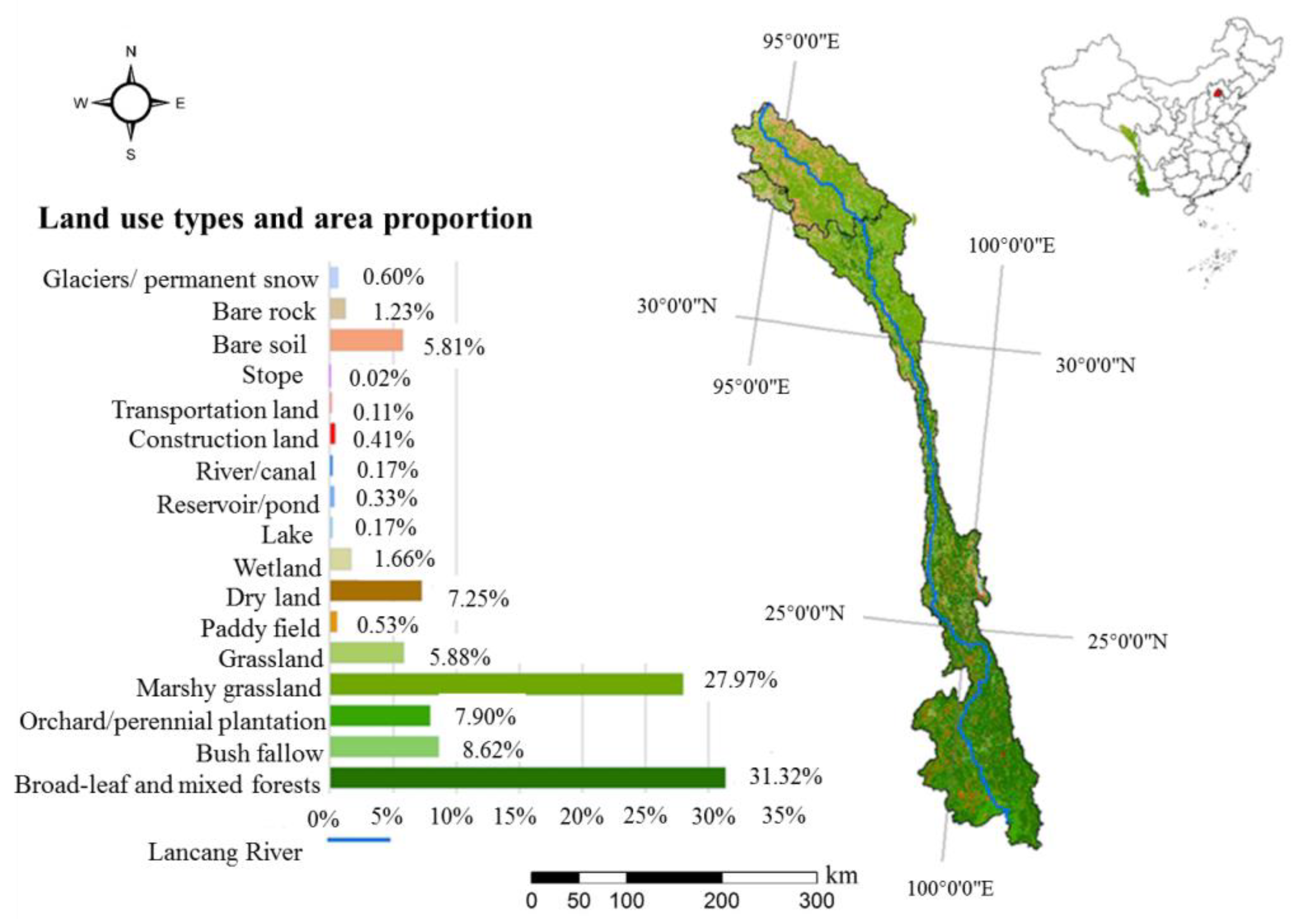
2.1. Study Area

The Lancang river valley is located in Southwest China (93°48′–101°48′ E, 21°07′–33°48′ N) with a total area of 165,383 km2 flowing through Qinghai, Tibet, Sichuan and Yunnan Province [34]. The valley is in the shape of a narrow strip in the north–south direction, wide upstream and downstream, and narrow midstream. The landform types are complex and diverse, and the upstream originates from the Qinghai–Tibet Plateau (QTP) with many alpine valleys. The midstream is hilly with a rugged terrain and multiple terraces, and the downstream is of alluvial plains with a flat terrain and frequent floods. The terrain is undulant with great spatial heterogeneity. The elevation in the upstream exceeds 4500 m and the relative vertical distance in the midstream is about 2000 m with a deep valley, while the terrain in the downstream is gentle and the minimum elevation is only 486 m.
The vertical difference in climate is remarkable. The upstream belongs to the alpine climate zone of the QTP with low temperature and low rainfall [35]. The mean annual temperature varies between −3 °C and 3 °C, and the mean annual precipitation ranges from 400 to 800 mm [35]. The midstream belongs to the subtropical climate of northwestern Yunnan, and the vertical change in temperature is obvious, which increases from north to south [36]. The mean annual temperature ranges between 12 °C and 15 °C, and the annual precipitation varies between 1000 and 2500 mm [36]. The downstream belongs to the tropical and subtropical climate of the southwestern Yunnan with temperatures increasing from north to south [37]. The mean annual temperature ranges between 15 °C and 22 °C, and the annual precipitation varies between 1000 and 3000 mm [37]. Overall, the whole basin belongs to the southwest monsoon climate with distinct dry and wet seasons [38]. The valley is very rich in water resources, and the mean annual runoff is approximately 4750 × 108 m3, which is about 9-fold greater than the annual runoff of the Yellow River [39]. The complex terrain and climate features form rich vegetation types with obvious latitude zonality and vertical zonality (Figure 1). Vegetation types mainly include alpine vegetation, meadows, shrubs, coniferous forests, broad-leaf and mixed forests, broad-leaf forests, cultivated vegetation and swamps, while meadows and shrubs are the main vegetation types of upstream [40]. The main land use types in the valley include agricultural land, forest land, grassland, urban land, water body, bare land and wetland. The proportion of cultivated land is relatively low, accounting for only 8.43% of the total area of the valley distributed in the downstream (Figure 1). Apart from that, there are large areas of bare rock and bare soil in the north part of the valley, accounting for 7.04% of the total area.

2.2. Data Sources and Processing

(1)
Land use and land cover.
In this study, land cover data with a 100 m × 100 m resolution in 2015 were provided by the Data Center for Resources and Environmental Sciences, Chinese Academy of Sciences (RESDC, Beijing) (http://www.resdc.cn, 1 September 2020). Based on the land cover data in 2015, we calculated the proportion of cultivated land and landscape pattern indexes, including the Largest Patch Index (LPI), Area Weighted Fractal Dimension of Patches (AWMPED) and Contagion Index (CONTAG) by Fragstats 4.2. Among them, LPI represents shape, AWMPED represents area and CONTAG represents aggregation aspects.
(2)
Gross Domestic Product (GDP) density.
In this study, GDP spatial distribution grid data with a 1 km × 1 km resolution in 2015 were provided by the Data Center for Resources and Environmental Sciences, Chinese Academy of Sciences (RESDC, Beijing) (http://www.resdc.cn, 5 September 2020).
(3)
Road and township data.
Township location point data were obtained from the GeoHey (https://geohey.com/, 10 September 2020). The road distribution data were obtained from the National Agriculture Science Data Sharing Center (http://www.agridata.cn, 8 September 2020).

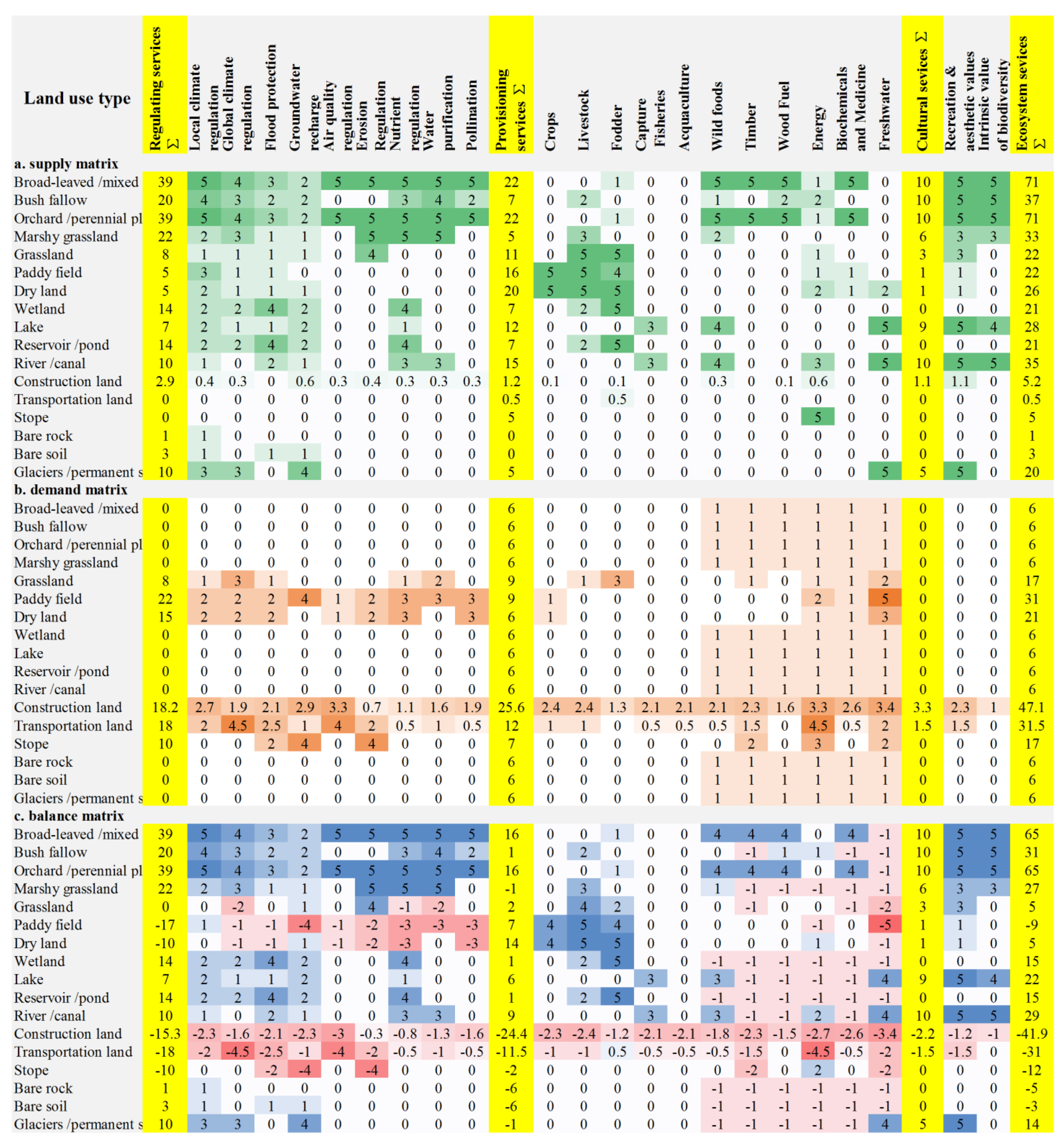
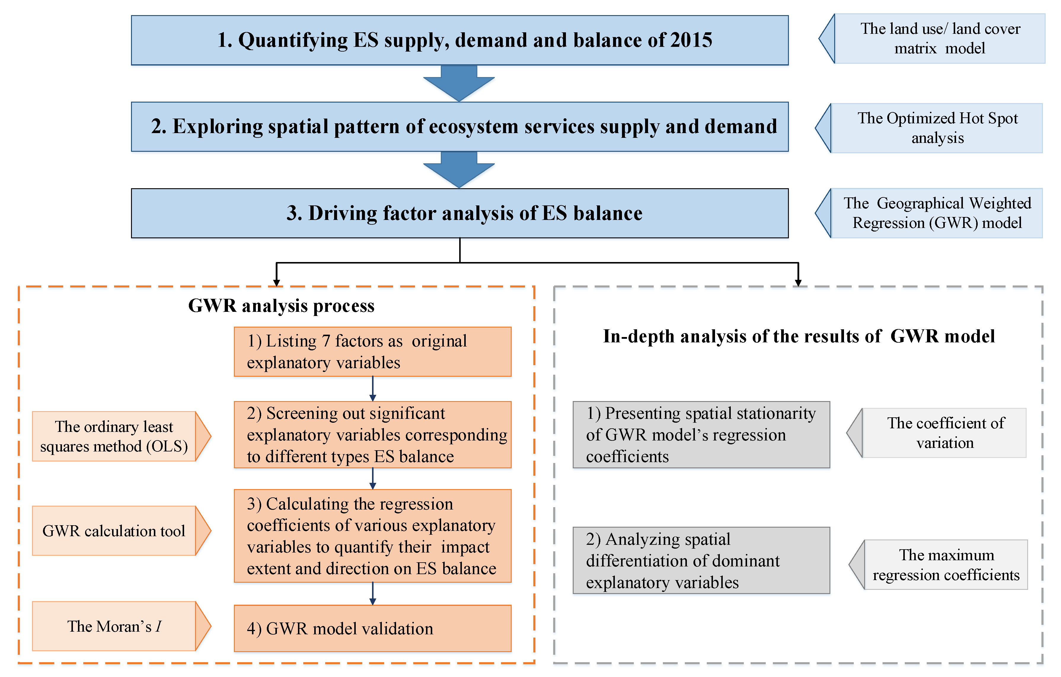
2.3. Quantification and Spatial Patterns of ES Supply, Demand and Balance

According to the LULC matrix model constructed by Burkhard et al., (2015) [8], we obtained the ES supply matrix and demand matrix by merging 44 land use types and 22 ES types of the original matrix into 25 land use types and 22 ES types (Figure 2). We assigned different values to the supply capacity and demand intensity of various ES types, including provisioning service (11 types), regulating service (9 types), and cultural service (2 types) for each land use type. The ES supply matrix was used to define the supply capacity of different land use types for various ESs (Figure 2a), while the ES demand matrix was used to reflect the actual demand intensity of humans for ESs for each land use type (Figure 2b). In these two matrixes, the evaluation levels of ES supply capacity and demand intensity vary from 0 to 5. It was reported that this method is a propagable and convenient method for ES quantification [3]. By subtracting the ES demand intensity by the ES supply capacity, we calculated the ES balance to identify the surplus and deficit of ES (Figure 2c). The evaluation scale ranges between −5 and 5. Negative values indicate that the demand for ESs exceeds the supply in a deficit state, and positive values indicate that ESs are in a surplus state. Based on the derived assessment matrixes of land use, the spatial quantitative analysis of ES supply, demand and balance of various ESs was carried out in the Lancang river valley. Then, the ES supply, demand, balance and total values were calculated by multiplying the area of 22 land use types by the quantitative values of ES supply, demand and balance to reflect the spatial variation of the ESs in the Lancang river valley. The formulas used are as follows:
E S j = i = 1 22 S i × V E S i   ( i = 1 ,   2 ,   3 .   22 )
    E S t o t a l = i = 1 3 E S j   (   j = 1 ,   2 ,   3 )
where VESi is the quantitative value of the ES category for land cover types i (i = 1, 2, 3… 22); Si is the area of land cover i; ESj is the ES value for ES categories j.
To verify the reliability of the method, the coefficient of sensitivity (CS) was further introduced to evaluate the response of total ES value to the change of the quantitative value. The formula used is as follows:
  C S = | ( E S V j E S V i ) / E S V i ( V C j k V C i k ) / V C i k |  
where i and j are the initial and adjusted values, respectively; adjustment quantity = ±50%; k is the land use type; VC is the quantitative value; and ESV is the total ES value. If CS ≥ 1, then ESV is flexible to VC, and the assessment method has poor accuracy and low credibility. If CS < 1, then ESV is inelastic to VC, and the method is credible.
In order to further explore the local performance of ES changes in space, Optimized Hot Spot analysis/Getis-Ord G* index in ArcGIS 10.5 was used to analyze the local correlation between coldspots and hotspots. The spatial pattern of the total ES supply and demand for each pixel (3 km × 3 km) was recognized to identify spatial clusters at a 99% significance level in the Lancang river valley in 2015. High-value clustered pixels were counted as hotspots; low-value clustered pixels were counted as coldspots; the high-value and low-value interval distributions were insignificant pixels. The formulas used are as follows:
  G i * = j = 1 n W i j X j X ¯ J = 1 n W i j S × [ n j = 1 n W i j 2 j = 1 n W i j ] 2 n 1
X ¯ = j = 1 n X j n
  S = j = 1 n X j 2 n 1 ( X ¯ ) 2
where W i j is the spatial weight; X i and X j are the observation values of the ith ESV evaluation unit and the jth ESV evaluation unit, respectively; and n is the sample size.

2.4. Driving Factor Analysis of ES Balance Based on Geographically Weighted Regression Model

The Geographical Weighted Regression (GWR) model is a kind of regression model that can detect the changes in the variable structure and variable relationship caused by geographical location changes, which is called spatial non-stationarity [41]. Compared with the general linear regression model, the GWR model effectively improves the goodness-of-fit, which has been widely used in spatial regression analysis [42,43,44]. The GWR model was calculated according to Equation (7) in ArcGIS 10.5.
  y i = β 0 ( u i , v i ) + i = 1 p β k ( u i , v i ) x i k + ε i
where ( u i , v i ) is the spatial position of the ith sample; x i k is the independent variable; β 0 ( u i , v i ) is the constant term estimate; β k ( u i , v i ) is the weight in the regression equation calculated according to the attenuation function, which is used to modify the parameter x i k ; p is the number of samples and ε i is the error correction term. The analysis process of the driving factor based on the GWR model is described as follows.
(1)
Driving factors screening.
In this study, 7 factors were initially selected to reflect human activity intensity as explanatory variables, including 4 direct reflection factors (GDP, cultivated land ratio, distance to road and distance to township point) and 3 indirect reflection factors describing the degree of landscape fragmentation (LPI, AWMPED and CONTAG). The balance values of four ES types were selected as the dependent variables, including regulating service balance, provisioning service balance, cultural service balance and total ES balance. In the GWR model, all variables were standardized, using the deviation standardization method.
(2)
GWR analysis process.
We divided the Lancang river valley into 18,325 grids (3 km × 3 km) and extracted the values of 4 dependent variables and 7 explanatory variables of each grid. Based on the above data, GWR analysis was performed in the 3 following steps:
Significant explanatory variables screening: The Ordinary Least Squares (OLS) method was used to carry out the regression analyses on 4 dependent variables and 7 explanatory variables to eliminate the insignificant variables and redundant variables, respectively. The screening criteria were that p-value was less than 0.05 and the Variance Inflation Factor (VIF) was less than 7.5. Then, OLS was performed again on the screened explanatory variables, and the obtained R2 was the goodness-of-fit of the global regression model. According to the OLS analysis, 4 corresponding explanatory variables were selected for provisioning service balance, including LPI, GDP, cultivated land ratio and distance to township points. For cultural services balance, 5 of the 7 corresponding explanatory variables (GDP, distance to road, distance to township point, LPI and AWMPED) were selected, except the CONTAG and cultivated land ratio. For regulating service balance and total ES balance, all of the 7 initial explanatory variables were screened out as corresponding explanatory variables.
GWR model performing: Using the Spatial Statistics/GWR tool in ArcGIS10.5, GWR model was respectively performed on 4 dependent variables and their corresponding explanatory variables. The weight function calibration method was adaptive, and the bandwidth determination method was AICc.
Moran’s I verification: The Spatial Autocorrelation (Moran’s I) tool was used to calculate the global Moran’s I of standardized residual in GWR model to test whether it was in a random distribution state.
(1)
Spatial stationarity analysis of GWR regression coefficients, and spatial differentiation analysis of dominant explanatory variables.
The coefficient of variation ( C v ) was calculated based on each regression coefficient in the GWR model to describe the spatial stationarity as follows:
C v = σ x ¯ × 100 %
where C v was the coefficient of variation; σ was the standard deviation; x ¯ was the average value.
The influence degree of various explanatory variables on ES balance value can be reflected by the regression coefficients of the pixel. In this study, we screened the maximum regression coefficients at pixel scale and performed the spatial differentiation analysis, which reflected the dominant explanatory variables of each pixel and their influence directions.
The research framework and corresponding methods were shown in Figure 3.

3. Results

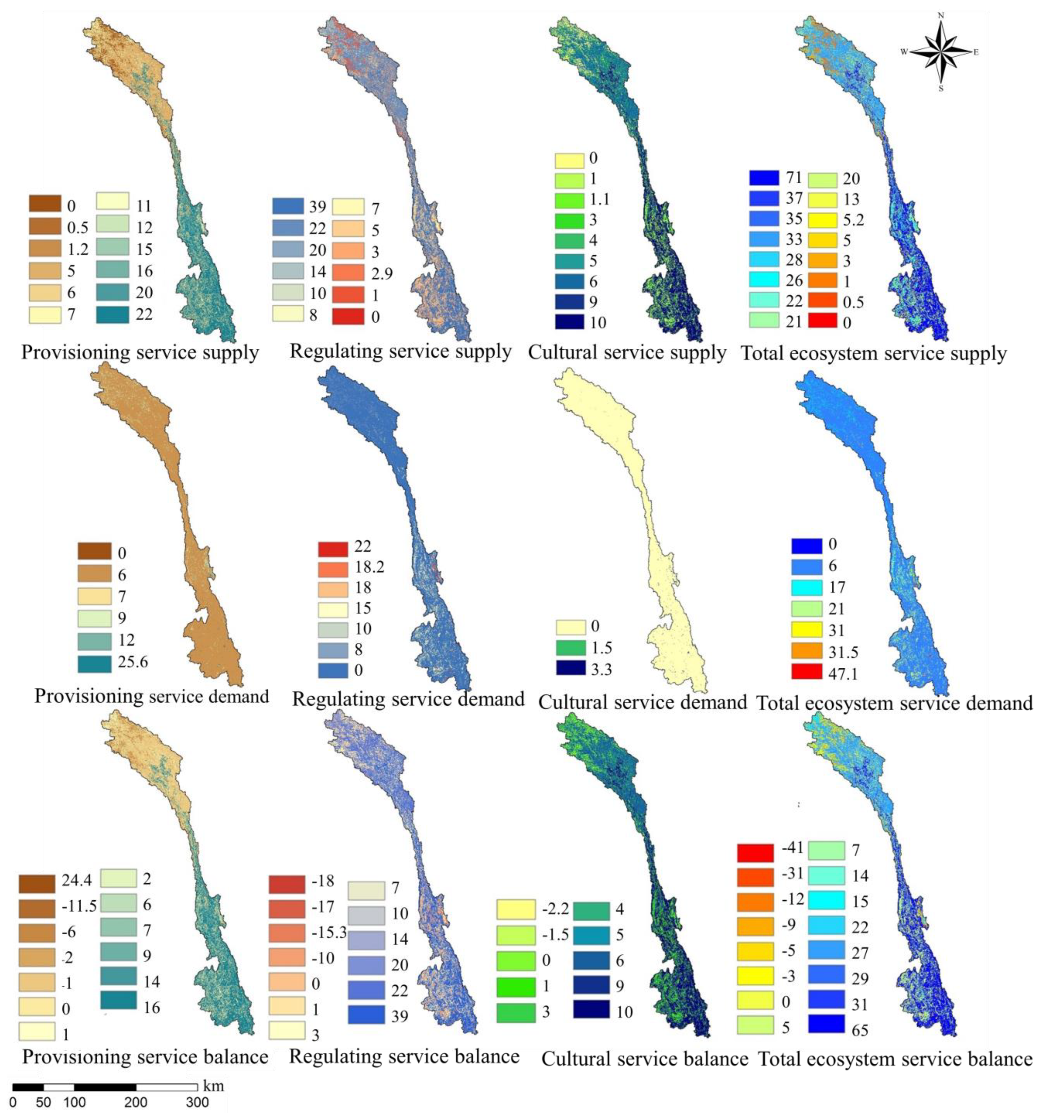
3.1. Spatial Distributions of ES Supply, Demand and Balance

As shown in Figure 4, the supply capacity of the provisioning service in the study area was low in the upstream and high in the downstream, similar to the spatial differentiation of elevation and climate [13,45]. The demand intensity of the provisioning service was generally low, and the high-value areas were scattered in the downstream, mainly in the Dali and Xishuangbanna cities. The deficit areas of provisioning service showed a continuous distribution in the upstream and a scattered distribution in the downstream. For regulating service, the supply capacity was overall high, and the low-value areas were mainly distributed in the Yushu, Puer and Lincang cities. The demand intensity of the regulating service was overall low with higher values in the downstream than in the upstream. Dali was the region where the high value of demand intensity was relatively concentrated. For cultural service, the supply capacity was high, especially in the southeastern part of the downstream, including Xishuangbanna and Puer. The demand of cultural service was low scattered in the whole study area. For total ES, the spatial characteristics of supply capacity was high in the downstream and low in the upstream. Although the demand intensity of total ES was also high in the downstream, the surplus of the downstream was much higher than that of the upstream, with only a small number of deficit areas scattered. In the upstream, deficit areas of total ES had a continuous distribution, but the degree of deficit was relatively low.

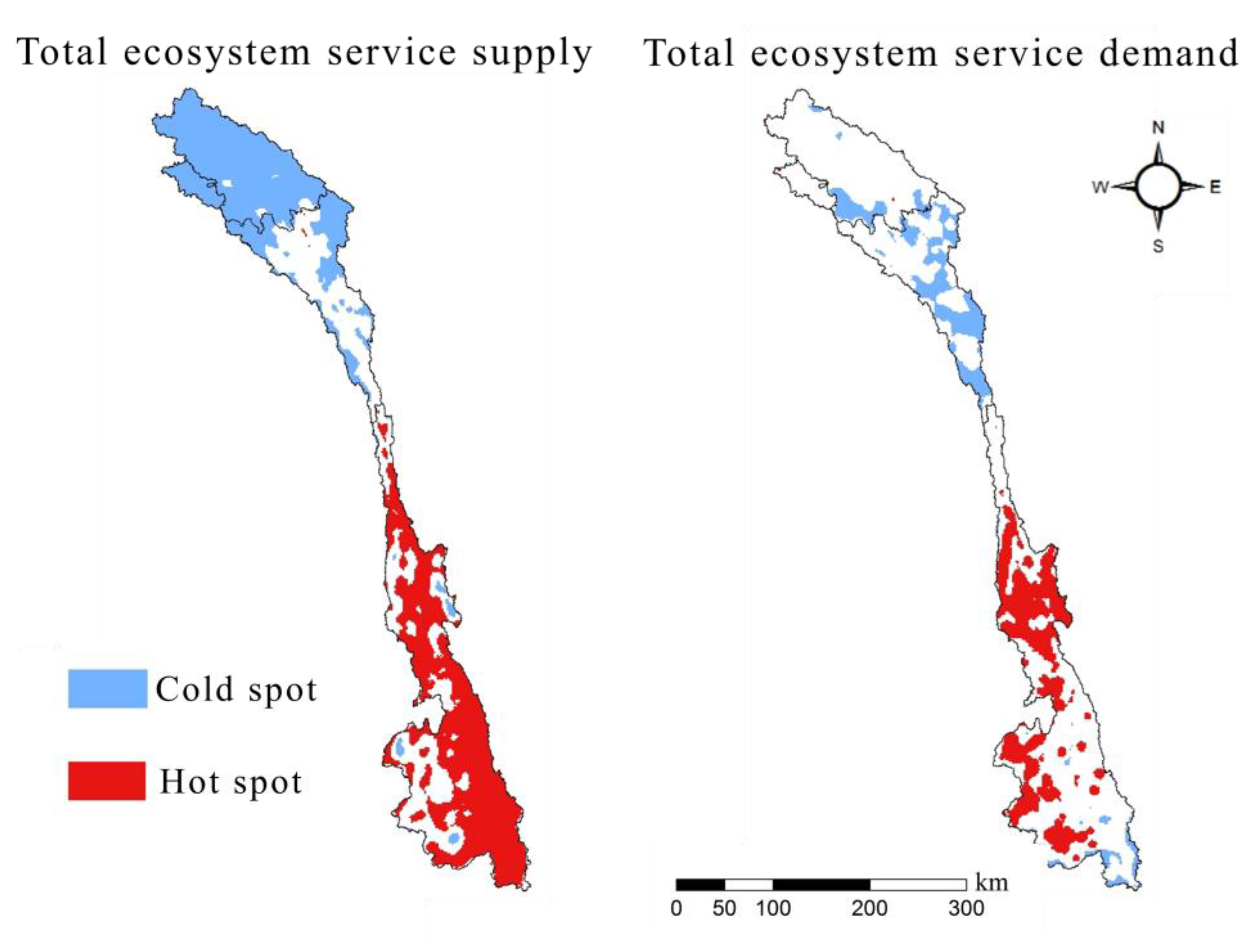
3.2. Spatial Patterns of Total ES Supply and Demand

The supply and demand of total ES in the study area were in a local, spatial aggregation pattern, as shown in Figure 5. For the total ES supply, the area of hotspots accounted for 35.87% of the Lancang river valley, concentrated in the eastern part of the downstream and scattered in the west. The area of coldspots accounted for 34.79% of the study area, concentrated in the upstream and scattered in the downstream. Compared with the total ES supply, the hotspots and coldspots of total ES demand represented a more dispersed distribution, being mainly distributed in Dali city and Nujiang Lisu Autonomous Prefecture with a small amount distributed in the western part of the downstream. The area of demand hotspots accounted for 18.84% of the total area. The number of coldspots was small, accounting for 13.71% of the study area, scattered in the Yushu and Changdu cities located in the upstream. When comparing the spatial pattern of the total ES supply with that of demand, the distribution of supply coldspots was more concentrated and northerly than that of demand coldspots. Both supply hotspots and demand hotspots were distributed in the downstream, representing mosaic distribution in the east–west direction, which explained the large spatial differences of total ES balance in the southern part of the study area.

3.3. Driving Factors Analysis of ES Balance Based on the OLS and GWR Models

3.3.1. OLS Analysis and Corresponding Explanatory Variable Selection

Comparing the OLS results of four dependent variables revealed that LPI was the major impact factor of all dependent variables (Table 1). The correlation coefficients were all greater than 0.7 and all were negatively impacted.

3.3.2. Validation of GWR Model and Spatial Stationarity of Explanatory Variables

Comparing the adjusted R2 of GWR and OLS demonstrated that the goodness-of-fit values of GWR models were higher than those of the corresponding OLS models in various ESs, indicating that the regression effect of the GWR model was better than that of the OLS model (Table 1). Meanwhile, based on the global Moran’s I, the z-scores of all four dependent variables were less than 1.65 and p-values were greater than 0.1, indicating that the standardized residuals showed random distribution and the GWR models passed the validation of the global Moran’s I (Table 1).
For the explanatory variables in the GWR model, the smaller the C v of the regression coefficient was, the larger the spatial stationarity and the more stable impact on ES balance were. In contrast, the larger C v was, the greater the fluctuation in space was and the more unstable the impact was. For different dependent variables, the spatial stationarity of different explanatory variables was as follows: (i) for the provisioning services balance, the explanatory variable with the largest spatial variability was GDP and the most stable explanatory variable was LPI; (ii) for the regulating services balance, the spatial stationarity of different explanatory variables was not much different, but the ratio of cultivated land showing the highest stability, and the explanatory variable with the largest spatial variability was GDP; (iii) for the cultural services balance, the spatial variabilities of the distance to road and distance to township points were the largest; and (iv) for the total ES balance, the explanatory variables with the largest spatial variabilities were GDP and AWMPED (Table 1).

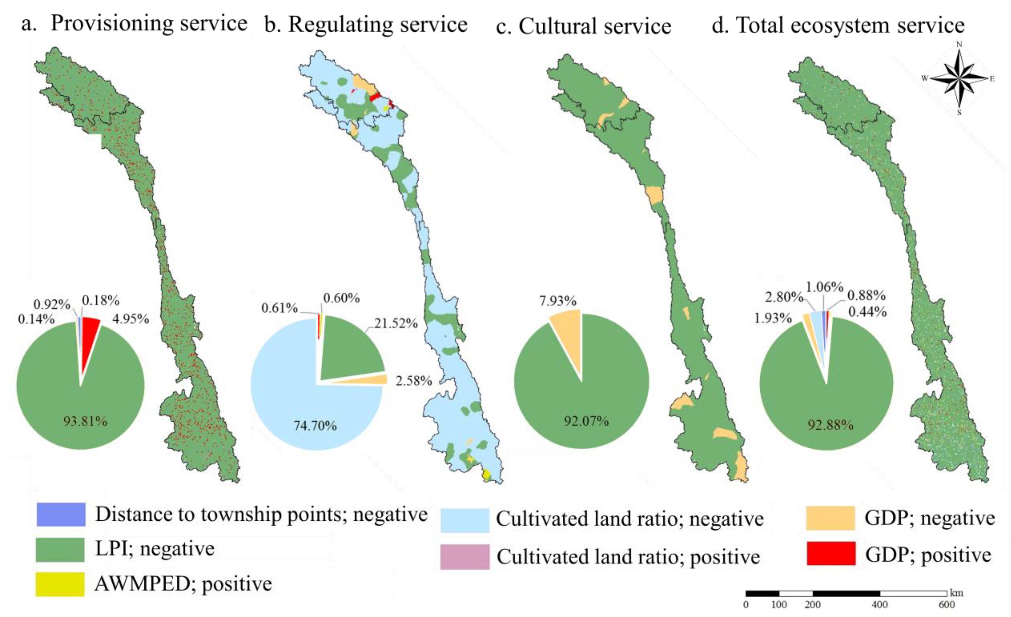
3.3.3. Spatial Differentiation Analysis of Dominant Explanatory Variables

The screening results of dominant explanatory variables at pixel scale indicated that four kinds of ES balance were affected by seven types dominant explanatory variables with negative or positive directions (Figure 6). For provisioning service balance, 93.81% of the pixels were negatively affected by LPI, and 4.95% of the pixels were positively affected by GDP. The remaining 1.24% of the pixels were affected by the other three variables. For regulating service balance, 74.70% of the pixels were negatively affected by the cultivated land ratio and 21.52% of the pixels were negatively affected by LPI. In addition, 2.58% of the pixels were negatively affected by GDP, concentrated in Yushu city. Cultural service balance only had two dominant explanatory variables. Specifically, 92.07% of the pixels were negatively affected by LPI, and the remaining pixels were negatively affected by GDP. The dominant explanation variables of total ES balance included six types, and 92.88% of the pixels were negatively affected by LPI. Overall, the impact of human activities on all kinds of ES balance was basically negative. Only the GDP, cultivated land ratio and AWMPED showed a positive influence on a few pixels.

4. Discussion

4.1. Spatial Variability of the ESs in the Lancang River Valley

The spatial patterns of the ESs indicated that the supply, demand and balance of various ESs presented low values in the upstream and high values in the downstream, which showed similar trends to the topographic and climatic distribution characteristics in study area [13,45]. The fundamental reason was that the spatial distribution of land use types is restricted by both natural conditions and human activities [46]. The restriction of natural conditions brought by the topographic and climatic features, and the contradictions between human and land jointly affected the land use status, thereby influencing the ES supply and demand [47].
Previous studies focusing on the values of ESs have proved that the ES values presented a regular distribution on the topographic and climatic gradients, which were affected by both elevation, slope, temperature and precipitation [45,48]. Taking the upper stream of the Min river as the study area, Zhu et al., (2017) analyzed the impact of the terrain niche on the ES values from the perspective of the selectivity of various land use types on topography [49]. Their results showed that, driven by the topography limitation and the human–land contradiction, the woodland and cultivated land with better topographic conditions were occupied by construction land, grassland and water, and the ES values varied in an inverted “V” shape with the rising topography [49]. Fang et al., (2020) quantified ES variations in elevation-associated vegetation types in a tropical region of China and found that ESs showed spatial differences along with different elevation levels in the Xishuangbanna area [47]. Furthermore, Jiang et al., (2016) assessed the ecosystem changes in the Three-River Headwater Region, and found that the increasing precipitation-intensified water erosion, and elevating temperature-induced glacier melting and permafrost degradation pose a threat to the ESs [50]. Lin et al., (2015) also concluded that climate, topography, land-use patterns and vegetation cover, as well as the interactions among them were the main factors that affected the spatial patterns of soil retention ESs in the Three Parallel Rivers Region [30].
The elevation is high in the upstream of the study area, and the midstream has a large elevation drop and steep slope, and the elevation in the downstream is constant. Thus, due to the undulating terrains, the land use types vary greatly in different parts of the Lancang river valley. Integrated with the driving effects of human activities, the study area forms the following land use characteristics: the downstream is mainly covered by woodland, construction land and cultivated land, and the upstream is mostly covered by grassland, bare soil and bare rock. Our study revealed the spatial variability of ESs at the watershed scale and found that the land use characteristics affect the spatial distribution of ES supply, demand and balance, similar to the distribution of topographic features [47].

4.2. Links between Landscape Pattern Indices on ES Balance

Landscape patterns can quantify the landscape structural composition and spatial configuration to reflect landscape dynamics and the ecological process [51]. Landscape composition and configuration impact the ability of ecosystems to provide goods and services, and the improvement or degradation in ESs can be detected by landscape pattern changes [52,53]. Landscape pattern indexes may be a valid tool to explore the effects of land-use changes and human activities on ESs [54,55]. The landscape pattern changes will affect the variation in landscape indexes and, thus, affect the change in ES supply and demand [56]. Therefore, combining landscape pattern indexes and ESs will contribute to exploring how landscape patterns influence the ES balance.
The results of our study showed that the ES balance was significantly correlated with the landscape pattern indexes, including LPI, AWMPED and CONTAG (Table 1). LPI was the dominant explanatory variable of ES balance for the majority pixels, characterized by strong influence and high spatial stability (Figure 6). Previous studies proved that the changes of landscape patterns had a regional impact on ES values [57]. Wang et al. found that there were significant positive correlations between ES values and landscape richness and aggregation, which showed a strong negative correlation between ES values and the complexity of patch shape [58]. The reliable links between landscape indexes and ESs in terms of land pattern and their implications should still be determined. In addition, the landscape patterns play a key role in the spatial variation of ES balance (Figure 6), consistent with the results of previous studies [52,59]. Yushanjiang et al. also quantified the spatial correlations between landscape patterns and ES values in Ebinur Lake Basin, Xinjiang, and their results showed that landscape metrics had direct spatial correlations with different ES types [52]. LPI had negative correlation with various ES balances, which can influence landscape fragmentation and connectivity [60,61]. It has been proved that social policies can effectively drive changes in landscape patterns, thus affecting the ES supply and demand [62]. Results of this research may provide scientific support for the formulation of regional ecosystem management policies from landscape perspectives.

4.3. Application and Advantages of GWR Model

Recently, several studies have proved that human activities and landscape patterns are important factors influencing ES supply, demand and balance [51,55]. Our results contributed to providing effective information and guidance for ES management. Previous studies on the driving factors of ESs focused on traditional analyses, such as correlation analysis, cluster analysis (CA) and principal component analysis (PCA) [63]. These methods could infer a preliminary assessment result about which human activity factors will have significant influence on ES balance. However, these studies lacked exploring the spatial distribution features of human activity factors’ effects on ES balance on a pixel scale, so they could not screen out the specific sites and types of human activity on spatial scale.
In this study, we used the OLS and GWR models to evaluate the driving influence of different human activity factors and landscape pattern indexes on ES balance, which could supply more detailed information for policy decision-making. The results of the OLS model showed that LPI had the greatest negative influence on various service types of ES balance, which has been proved by the front section. In agreement with the OLS model analysis, the GWR model also revealed that LPI showed the strongest negative effect on ES balance for the majority of the pixels (Figure 6). However, the difference between these two methods was that the GWR model could determine the weight of each sample point in the regression equation by establishing the distance attenuation function, whereas the OLS analysis could not. The constructed local regression equation conformed to the first law of geography and showed a higher goodness-of-fit than that of the OLS model (Table 1), which was consistent with the results of previous studies [42,44]. For example, Wu (2020) explored the spatio-temporal variations of the ecological footprint and its influencing factors in China’s provinces using the GWR model and concluded that the GWR model was superior to OLS considering the regression analysis of the goodness-of-fit, variance comparisons and the spatial auto-correlation of residual [42]. In addition, compared with global regression, the GWR model can obtain the influence degree of different human activity factors on the ES balance at pixel scale. All these findings imply the advantages of the GWR model over the OLS model in exploring the spatial distribution and driving force of ES balance at regional and spatial scales. By screening the dominant explanatory variables, the results can provide more detailed and effective guidance for the regulation of regional ESs.

4.4. Limitations and Implications for Ecological Management at the Watershed Scale

In this study, we applied the LULC matrix model to quantify and map ES supply, demand and balance in the Lancang river valley. According to the previous studies, due to the simplicity, the LUCC matrix method has been widely applied to quantify ES supply, demand and balance in many areas [2,8,64]. However, there are some uncertainties and criticisms for this method. This method was an expert-based evaluation method with high subjective limitations and lacked conformity [65]. Only land-use data were used in the ES assessment, but other influencing factors, such as population and GDP, were ignored, which may bring estimation mistakes. These above uncertainties would bring uncertain results for ES balance estimation with great discrepancies [7]. Thus, we further calculated the CS to verify the reliability of the LULC assessment method. The results showed that the CS values for various land use types were less than 1, which indicated the rationality and reliability of our method and results [2,17]. Therefore, in future studies, all possible uncertainties should be further considered at watershed scale to provide more valid assessment and support for ES management at the watershed scale.
In addition, many human activity factors and landscape indexes, namely GDP, cultivated land ratio, distance to road, distance to township point, LPI, AWMPED and CONTAG, have been used to explore the driving forces of ES balance in the Lancang river valley. These factors are some representative factors that we selected to better reflect the human activity intensity in the study. In previous studies, Zhao et al., (2015) selected population density, number of villages and road length to evaluate the human influence intensity on the QTP [66]; Li et al., (2018) introduced the electricity infrastructure, population density, land use intensity, road and railways, and grazing intensity to reflect human activity [27] but these human activity factors are insufficient. In addition, GDP, cultivation activity and landscape pattern indexes may be also important factors influencing human activity [3,52]. Therefore, compared to previous studies, we had a comprehensive consideration for the influence of human activities on ESs, which provided more reliable results. However, some other human activity and landscape factors may also influence the ES balance, such as population density, traffic volume, night-time light and tourism belonging to human activity factors, and patch density (PD), landscape division index (DIVISION) and landscape shape index (LSI) belonging to landscape pattern indexes [27,52,57]. The inadequate consideration of these impact factors in the Lancang river valley may underestimate the assessment results. Many studies showed that tourism and traffic volume would bring a significant and negative influence on ESs [67,68], but these data are usually difficult to obtain at watershed scale; thus, we excluded the data. Many potential human activity factors may threaten the ecosystem, thus more attention should be paid to consider all the possible factors of human activity intensity at the watershed scale in future studies.

5. Conclusions

Regional land use status is an important factor driving the change in ES supply and demand. In this study, based on the LULC matrix model, four kinds of ES supply, demand and balance in the Lancang river valley were quantified, and the spatial distribution maps of various ESs were obtained. On this basis, we analyzed the spatial pattern of total ES supply and demand and obtained the quantity and spatial characteristics of the hotspots and coldspots of total ES supply and demand, which performed as hotspots in the south and coldspots in the north. Furthermore, using the OLS and GWR models, we conducted a driving factor analysis on various ES balances, and screened human activity factors with significant influence. According to the regression coefficients of each explanatory variable, the dominant explanatory variables of each pixel were obtained. The results showed that the provisioning service and cultural service of the ES balance were significantly affected by four and five human activity factors, respectively, and regulating service of the ES balance and total ES balance were significantly affected by seven human activity factors. Among the factors, LPI was proved to be the dominant explanatory variable of the vast majority pixels and its influence direction was negative. The research also indicated that the impacts of human activities on various service types of ES balances were basically negative, and only GDP, cultivated land ratio and AWMPED had a positive influence on a small quantity of pixels. The research may provide scientific support for regional ES management and regulation.

Author Contributions

S.L.: Conceptualization, funding acquisition, visualization; Y.S.: Writing—review and editing, software, X.W.: Writing—original draft, software; W.L.: Visualization; Y.L.: Methodology; L.-S.P.T.: Validation, editing and revising. All authors have read and agreed to the published version of the manuscript.

Funding

The work was supported by the second scientific expedition to the Qinghai–Tibet Plateau (No. 2019QZKK0405-05), National Natural Sciences Foundation of China (No. 41571173) and National Key Research and Development Project (No. 2016YFC0502103).

Institutional Review Board Statement

Not applicable.

Informed Consent Statement

Not applicable.

Data Availability Statement

The data generated for this study are available on Dryad (https://0-doi-org.brum.beds.ac.uk/10.5061/dryad.d51c5b01h, 17 September 2020).

Acknowledgments

We would like to acknowledge all the teachers and students who participated in the data downloading and processing, and wrote, revised and reviewed the original draft.

Conflicts of Interest

The authors declare no conflict of interest.

References

  1. Xiao, Y.; Xie, G.; Lu, C.; Xu, J. Involvement of ecosystem service flows in human wellbeing based on the relationship between supply and demand. Sci. Total Environ. 2016, 36, 3096–3102. [Google Scholar]
  2. Sun, Y.; Liu, S.; Dong, Y.; An, Y.; Shi, F.; Dong, S.; Liu, G. Spatio-temporal evolution scenarios and the coupling analysis of ecosystem services with land use change in China. Sci. Total Environ. 2019, 681, 211–225. [Google Scholar] [CrossRef]
  3. Sun, Y.; Liu, S.; Shi, F.; An, Y.; Li, M.; Liu, Y. Spatio-temporal variations and coupling of human activity intensity and ecosystem services based on the four-quadrant model on the Qinghai-Tibet Plateau. Sci. Total Environ. 2020, 743, 140721. [Google Scholar]
  4. James, B.; Banzhaf, S. What are ecosystem services? The need for standardized environmental accounting units. Ecol. Econ. 2007, 63, 616–626. [Google Scholar]
  5. Pearson, C. The economics of ecosystems and biodiversity: Ecological and economic foundations. J. Environ. Manag. 2012, 19, 68–69. [Google Scholar]
  6. Xie, G.; Cao, S.; Lu, C.; Xiao, Y.; Zhang, Y. Human’s consumption of ecosystem services and ecological debt in China. J. Nat. Resour. 2010, 25, 43–51. [Google Scholar]
  7. Burkhard, B.; Kroll, F.; Nedkov, S.; Müller, F. Mapping ecosystem service supply, demand and budgets. Ecol. Indic. 2012, 21 (Suppl. C), 17–29. [Google Scholar] [CrossRef]
  8. Burkhard, B.; Müller, A.; Müller, F.; Grescho, V.; Anh, Q.; Arida, G.; Bustamante, J.V.; van Chien, H.; Heong, K.; Escalada, M.; et al. Land cover-based ecosystem service assessment of irrigated rice cropping systems in southeast Asia—An explorative study. Ecosyst. Serv. 2015, 14, 76–87. [Google Scholar] [CrossRef]
  9. Bai, Y.; Wang, M.; Li, H.; Huang, S.; Alatalo, J.M. Ecosystem service supply and demand: Theory and management application. Sci. Total Environ. 2017, 37, 5846–5852. [Google Scholar]
  10. Xie, G.; Zhen, L.; Lu, C.; Xiao, Y.; Chen, C. Expert knowledge based valuation method of ecosystem services in China. J. Nat. Resour. 2008, 23, 911–919. [Google Scholar]
  11. Xie, G.; Zhang, C.; Zhang, L.; Chen, W.; Li, S. Improvement of the evaluation method for ecosystem service value based on per unit area. J. Nat. Resour. 2015, 30, 1243–1254. [Google Scholar]
  12. Ma, C.; Wang, X.; Zhang, Y.; Li, S. Emergy analysis of ecosystem services supply and flow in Beijing ecological conservation area. Acta Geogr. Sin. 2017, 72, 974–985. [Google Scholar]
  13. Jiang, B.; Chen, Y.; Xiao, Y.; Zhao, J.; Ouyang, Z. Evaluation of the economic value of final ecosystem services from the Baiyangdian wetland. Sci. Total Environ. 2017, 37, 2497–2505. [Google Scholar]
  14. Bukvareva, E.; Zamolodchikov, D.; Kraev, G.; Grunewald, K.; Narykov, A. Supplied, demanded and consumed ecosystem services: Prospects for national assessment in Russia. Ecol. Indic. 2017, 78, 351–360. [Google Scholar] [CrossRef]
  15. Tolessa, T.; Senbeta, F.; Kidane, M. The impact of land use/land cover change on ecosystem services in the central highlands of Ethiopia. Ecosyst. Serv. 2017, 23, 47–54. [Google Scholar] [CrossRef]
  16. Burkhard, B.; Kroll, F.; Müller, F.; Windhorst, W. Landscapes’ capacities to provide ecosystem services—A concept for land-cover based assessments. Landsc. Online 2009, 15, 1–22. [Google Scholar] [CrossRef]
  17. Wu, X.; Liu, S.; Zhao, S.; Hou, X.; Xu, J.; Dong, S.; Liu, G. Quantification and driving force analysis of ecosystem services supply, demand and balance in China. Sci. Total Environ. 2019, 652, 1375–1386. [Google Scholar] [CrossRef]
  18. Yan, Y.; Zhu, J.; Wu, G.; Zhan, Y. Review and prospective applications of demand, supply, and consumption of ecosystem services. Sci. Total Environ. 2017, 37, 2489–2496. [Google Scholar]
  19. Lin, J.; Huang, J.; Prell, C.; Bryan, B.A. Changes in supply and demand mediate the effects of land-use change on freshwater ecosystem services flows. Sci. Total. Environ. 2021, 763, 143012. [Google Scholar] [CrossRef]
  20. Xu, J.; Chen, J.; Liu, Y. Partitioned responses of ecosystem services and their tradeoffs to human activities in the Belt and Road region. J. Clean. Prod. 2020, 276, 123205. [Google Scholar]
  21. Wu, L.; Yang, S.; Liu, X.; Luo, Y.; Zhou, X.; Zhao, H. Response analysis of land use change to the degree of human activities in Beiluo River basin since 1976. Sci. Total Environ. 2014, 69, 54–63. [Google Scholar]
  22. Zang, Z.; Zou, X.; Zuo, P.; Song, Q.; Wang, C.; Wang, J. Impact of landscape patterns on ecological vulnerability and ecosystem service values: An empirical analysis of Yancheng Nature Reserve in China. Ecol. Indic. 2017, 72, 142–152. [Google Scholar] [CrossRef]
  23. Kain, J.-H.; Larondelle, N.; Haase, D.; Kaczorowska, A. Exploring local consequences of two land-use alternatives for the supply of urban ecosystem services in Stockholm year 2050. Ecol. Indic. 2016, 70, 615–629. [Google Scholar] [CrossRef]
  24. Kim, J.H.; Jobbágy, E.G.; Jackson, R.B. Trade-offs in water and carbon ecosystem services with land-use changes in grasslands. Ecol. Appl. 2016, 26, 1633–1644. [Google Scholar] [CrossRef] [PubMed] [Green Version]
  25. Nicholson, C.C.; Koh, I.; Richardson, L.L.; Beauchemin, A.; Ricketts, T.H. Farm and landscape factors interact to affect the supply of pollination services. Agric. Ecosyst. Environ. 2017, 250, 113–122. [Google Scholar] [CrossRef]
  26. Rong, Y.; Li, C.; Xu, C.; Yan, Y. Ecosystem service values and spatial differentiation changes during urbanization: A case study of Huanghua City. Chin. J. Ecol. 2017, 36, 1374–1381. [Google Scholar]
  27. Li, S.; Zhang, Y.; Wang, Z.; Li, L. Mapping human influence intensity in the Tibetan Plateau for conservation of ecological service functions. Ecosyst. Serv. 2018, 30, 276–286. [Google Scholar] [CrossRef]
  28. Fan, N.; Xie, G.; Zhang, C.; Chen, L.; Li, W.; Cheng, S. Spatial-temporal dynamic changes of vegetation cover in Lancang River Basin during 2001–2010. Resour. Sci. 2012, 34, 1222–1231. [Google Scholar]
  29. Zhang, B.; Ding, W.; Xu, B.; Wang, L.; Li, Y.; Zhang, C. Spatial characteristics of total phosphorus loads from different sources in the Lancang River Basin. Sci. Total Environ. 2020, 722, 137863. [Google Scholar] [CrossRef]
  30. Lin, S.; Wu, R. The spatial pattern of soil retention ecosystem service in the Three Parallel Rivers Region. J. Yunnan Univ. Nat. Sci. 2015, 37, 295–302. [Google Scholar]
  31. Han, Z.; Song, W.; Deng, X.; Xu, X. Trade-Offs and Synergies in Ecosystem Service within the Three-Rivers Headwater Region, China. Water 2017, 9, 588. [Google Scholar] [CrossRef] [Green Version]
  32. Zhang, Y.; Hou, J.; Ma, G.; Zhai, X.; Lv, A.; Wang, W.; Wang, Z. Regional differences of water regulation services of terrestrial ecosystem in the Tibetan Plateau: Insights from multiple land covers. J. Clean. Prod. 2021, 283, 125216. [Google Scholar]
  33. Zhang, J.; Feng, Z.; Jiang, L.; Yang, Y.; Liu, X. Effect of road disturbance on landscape pattern in the Lancang River Valley. J. Nat. Resour. 2013, 28, 969–980. [Google Scholar]
  34. Chen, L.; Zhang, C.; Xie, G.; Liu, C.; Wang, H.; Li, Z.; Pei, S.; Qiao, Q. Vegetation Carbon Storage, Spatial Patterns and Response to Altitude in Lancang River Basin, Southwest China. Sustainability 2016, 8, 110. [Google Scholar] [CrossRef] [Green Version]
  35. Ouyang, W.; Wan, X.; Xu, Y.; Wang, X.; Lin, C. Vertical difference of climate change impacts on vegetation at temporal-spatial scales in the upper stream of the Mekong River Basin. Sci. Total Environ. 2020, 701, 134782. [Google Scholar] [CrossRef]
  36. Liu, S.; An, N.; Dong, S.; Zhao, C.; Coxixo, A.; Cheng, F.; Hou, X. Spatial variations of sedimentary organic carbon associated with soil loss influenced by cascading dams in the middle Lancang River. Ecol. Eng. 2017, 106, 323–332. [Google Scholar] [CrossRef]
  37. Juan, W.; Baoshan, C.; Huarong, Y. Spatio-temporal dynamic study on landscape patterns in Lancang River watershed of Yunnan province. J. Soil Water Conserv. 2007, 21, 85–89; 97. [Google Scholar]
  38. Yun, X.; Tang, Q.; Wang, J.; Liu, X.; Zhang, Y.; Lu, H.; Wang, Y.; Zhang, L.; Chen, D. Impacts of climate change and reservoir operation on streamflow and flood characteristics in the Lancang-Mekong River Basin. J. Hydrol. 2020, 590, 125472. [Google Scholar] [CrossRef]
  39. Tan, X.; Wang, J.; Tang, X.; Yang, N.; Luo, X.; Li, Y.; Wang, G. Variation trends of climate change and hydrological responses of individual regions in Lancang -Mekong River Basin from 1960–2012. J. Water Resour. Water Eng. 2020, 31, 1–8. [Google Scholar]
  40. Liu, S.; Dong, Y.; Deng, L.; Liu, Q.; Zhao, H.; Dong, S. Forest fragmentation and landscape connectivity change associated with road network extension and city expansion: A case study in the Lancang River Valley. Ecol. Indic. 2014, 36, 160–168. [Google Scholar] [CrossRef]
  41. Fotheringham, A.S.; Charlton, M.; Brunsdon, C. The geography of parameter space: An investigation of spatial non-stationarity. Int. J. Geogr. Inform. Syst. 1996, 10, 605–627. [Google Scholar] [CrossRef]
  42. Wu, D. Spatially and temporally varying relationships between ecological footprint and influencing factors in China’s provinces Using Geographically Weighted Regression (GWR). J. Clean. Prod. 2020, 261, 121089. [Google Scholar] [CrossRef]
  43. Sheng, J.; Han, X.; Zhou, H. Spatially varying patterns of afforestation/reforestation and socio-economic factors in China: A geographically weighted regression approach. J. Clean. Prod. 2017, 153, 362–371. [Google Scholar] [CrossRef]
  44. Zhao, R.; Zhan, L.; Yao, M.; Yang, L. A geographically weighted regression model augmented by Geodetector analysis and principal component analysis for the spatial distribution of PM2.5. Sustain. Cities Soc. 2020, 56, 102106. [Google Scholar] [CrossRef]
  45. Yang, S.H.; Hu, S.G.; Qu, S.J. Terrain gradient effect of ecosystem service value in middle reach of Yangtze River, China. Ying Yong Sheng Tai Xue Bao = J. Appl. Ecol. 2018, 29, 976–986. [Google Scholar]
  46. Gomes, L.C.; Bianchi, F.J.J.A.; Cardoso, I.M.; Filho, E.I.F.; Schulte, R.P.O. Land use change drives the spatio-temporal variation of ecosystem services and their interactions along an altitudinal gradient in Brazil. Landsc. Ecol. 2020, 35, 1571–1586. [Google Scholar] [CrossRef]
  47. Fang, Z.; Bai, Y.; Jiang, B.; Alatalo, J.M.; Liu, G.; Wang, H. Quantifying variations in ecosystem services in altitude-associated vegetation types in a tropical region of China. Sci. Total Environ. 2020, 726, 138565. [Google Scholar] [CrossRef]
  48. Wang, X.; Xue, Y.; Zhang, Y. Assessing the ecosystem service values in Shaanxi Province based on terrain. J. Glaciol. Geocryol. 2016, 38, 1432–1439. [Google Scholar]
  49. Zhu, C.; Zhang, J.; Zhao, Y.; Liu, C. Topographic gradient effects of typical watershed ecosystem services in the eastern Tibetan Plateau: A case study of the upper reaches of Minjiang River. Resour. Environ. Yangtze Basin. 2017, 26, 1687–1699. [Google Scholar]
  50. Jiang, C.; Zhang, L. Ecosystem change assessment in the Three-river Headwater Region, China: Patterns, causes, and implications. Ecol. Eng. 2016, 93, 24–36. [Google Scholar] [CrossRef]
  51. Zhang, J.; Qu, M.; Wang, C.; Zhao, J.; Cao, Y. Quantifying landscape pattern and ecosystem service value changes: A case study at the county level in the Chinese Loess Plateau. Glob. Ecol. Conserv. 2020, 23, e01110. [Google Scholar] [CrossRef]
  52. Yushanjiang, A.; Zhang, F.; Yu, H.; Kung, H.-T. Quantifying the spatial correlations between landscape pattern and ecosystem service value: A case study in Ebinur Lake Basin, Xinjiang, China. Ecol. Eng. 2018, 113, 94–104. [Google Scholar] [CrossRef]
  53. Estoque, R.C.; Murayama, Y. Quantifying landscape pattern and ecosystem service value changes in four rapidly urbanizing hill stations of Southeast Asia. Landsc. Ecol. 2016, 31, 1481–1507. [Google Scholar] [CrossRef]
  54. Su, S.; Xiao, R.; Jiang, Z.; Zhang, Y. Characterizing landscape pattern and ecosystem service value changes for urbanization impacts at an eco-regional scale. Appl. Geogr. 2012, 34, 295–305. [Google Scholar] [CrossRef]
  55. Zhao, Q.; Wen, Z.; Chen, S.; Ding, S.; Zhang, M. Quantifying Land Use/Land Cover and Landscape Pattern Changes and Impacts on Ecosystem Services. Int. J. Environ. Res. Public Health 2019, 17, 126. [Google Scholar] [CrossRef] [Green Version]
  56. Hou, L.; Wu, F.; Xie, X. The spatial characteristics and relationships between landscape pattern and ecosystem service value along an urban-rural gradient in Xi’an city, China. Ecol. Indic. 2020, 108, 105720. [Google Scholar] [CrossRef]
  57. Wu, J.; Li, Y. Variation of landscape pattern and its Influences on ecosystem service in value in Three Gorges Reservoir Area (Chongqing section). J. Ecol. Rural Environ. 2018, 34, 308–317. [Google Scholar]
  58. Wang, H.; Qin, F.; Zhu, J.; Zhang, C. The effects of land use structure and landscape pattern change on ecosystem service values. Sci. Total Environ. 2017, 37, 286–1296. [Google Scholar]
  59. Kindu, M.; Schneider, T.; Teketay, D.; Knoke, T. Changes of ecosystem service values in response to land use/land cover dynamics in Munessa–Shashemene landscape of the Ethiopian highlands. Sci. Total Environ. 2016, 547, 137–147. [Google Scholar] [CrossRef] [PubMed]
  60. Mitchell, M.G.; Bennett, E.M.; Gonzalez, A. Agricultural landscape structure affects arthropod diversity and arthropod-derived ecosystem services. Agric. Ecosyst. Environ. 2014, 192, 144–151. [Google Scholar] [CrossRef]
  61. Su, S.; Jiang, Z.; Zhang, Q.; Zhang, Y. Transformation of agricultural landscapes under rapid urbanization: A threat to sustainability in Hang-Jia-Hu region, China. Appl. Geogr. 2011, 31, 439–449. [Google Scholar] [CrossRef]
  62. Li, Y.; Chang, Y.; Hu, Y.; Ii, X.; Xiao, D. Research advance in effects of anthropogenic activity on forest landscape. Sci. Silvae Sin. 2006, 42, 119–126. [Google Scholar]
  63. Li, T.; Xiong, Q.; Luo, P.; Zhang, Y.; Gu, X.; Lin, B. Direct and indirect effects of environmental factors, spatial constraints, and functional traits on shaping the plant diversity of montane forests. Ecol. Evol. 2019, 10, 557–568. [Google Scholar] [CrossRef] [PubMed]
  64. Cai, W.; Gibbs, D.; Zhang, L.; Ferrier, G.; Cai, Y. Identifying hotspots and management of critical ecosystem services in rapidly urbanizing Yangtze River Delta Region, China. J. Environ. Manag. 2017, 191, 258–267. [Google Scholar] [CrossRef] [PubMed]
  65. Li, J.; Jiang, H.; Bai, Y.; Alatalo, J.M.; Li, X.; Jiang, H.; Liu, G.; Xu, J. Indicators for spatial–temporal comparisons of ecosystem service status between regions: A case study of the Taihu River Basin, China. Ecol. Indic. 2016, 60, 1008–1016. [Google Scholar] [CrossRef]
  66. Zhao, H.; Liu, S.; Dong, S.; Su, X.; Wang, X.; Wu, X.; Wu, L.; Zhang, X. Analysis of vegetation change associated with human disturbance using MODIS data on the rangelands of the Qinghai-Tibet Plateau. Rangel. J. 2015, 37, 77–87. [Google Scholar] [CrossRef]
  67. Gladstone, W.; Curley, B.; Shokri, M.R. Environmental impacts of tourism in the Gulf and the Red Sea. Mar. Pollut. Bull. 2013, 72, 375–388. [Google Scholar] [CrossRef] [PubMed]
  68. Theobald, D.M. Estimating natural landscape changes from 1992 to 2030 in the conterminous US. Landsc. Ecol. 2010, 25, 999–1011. [Google Scholar] [CrossRef]
Figure 1. Location and land use type distribution of study area.
Land 10 00522 g001
Figure 2. Assessment matrix of ES supply and demand for different land use types.
Land 10 00522 g002
Figure 3. Research framework and corresponding methods.
Land 10 00522 g003
Figure 4. Spatial distributions of ESs in the Lancang river valley.
Land 10 00522 g004
Figure 5. Local spatial patterns of ES supply and demand.
Land 10 00522 g005
Figure 6. Spatial differentiation of dominant explanatory variables.
Land 10 00522 g006
Table 1. Parameters and test results of OLS and GWR.
Balance TypeProvisioning ServicesRegulating ServicesCultural ServicesTotal ES Balance
OLSGWROLSGWROLSGWROLSGWR
1Largest Patch Index (LPI)−0.781 **0.191−6.350 **0.184−0.719 **0.11−0.767 **0.185
2Area Weighted Fractal Dimension of Patches (AWMPED)−0.024 **1.856−0.012 **1.932
3Contagion Index (CONTAG)−0.066 **0.8350.034 **0.8430.041 **1.281
4GDP−0.098 **13.786−0.086 **2.312−0.074 **0.593−0.098 **2.271
5The ratio of cultivated land0.077 **2.031−0.709 **0.167−0.454 **0.311
6Distance to road−0.041 **1.219−0.082 **1.488−0.032 **1.335
7Distance to township points0.024 **1.156−0.027 **0.927−0.085 **1.129−0.018 **0.99
8Adjusted R2 of OLS0.6310.6100.3790.570
9Adjusted R2 GWR0.7080.6600.3990.634
10Moran’s I-z-score0.409−1.324−1.561−0.814
11Moran’s I-p-value0.6830.1850.1180.416
** p < 0.01.
Publisher’s Note: MDPI stays neutral with regard to jurisdictional claims in published maps and institutional affiliations.

