1. Introduction
Land cover is defined as the biophysical cover of Earth’s surface, as artificial surfaces, agricultural areas, forests and semi-natural areas, water and wetlands by the Directive 2007/02 of the European Commission [
1,
2]. Different land cover types furnish various ecosystem services and support habitats; land cover is also considered a climate variable, an element for the description of the environment [
3]. Human activities depend on land cover and its evolution [
4]. Therefore, the comprehension of the processes that lead to the transformation of the territory are crucial for sustainable resource management, environmental protection, modelling of climate change scenarios, and for the assessment of the impacts on the earth system directly linked to human activities [
5]. Remote sensing is important to the study of Earth phenomena, which can be monitored and assessed at different spatial and temporal resolutions [
6,
7].
Several user communities such as decision-makers, non-governmental organizations, European communities, scientists and researchers require different types of land cover information for their activities and policies [
8]. For example, land cover information is used for evaluating progress towards UN Sustainable Development Goals (SDGs) targets [
9], such as target 15.3, which is related to the reach of the Land Degradation Neutrality (LDN) by 2030 [
10]. Despite the importance of land cover data in environmental monitoring and planning, the products currently available on a national scale are limited in number and their characteristics are not always adequate. The main national land cover and land use products are part of the Copernicus program (
https://land.copernicus.eu, accessed on 28 February 2021). The CORINE Land Cover (CLC) guarantees a high thematic detail and a long historical series, but is limited from the point of view of spatial detail and updating frequency (
https://land.copernicus.eu/pan-european/corine-land-cover, accessed on 28 February 2021). More recently, the High Resolution Layers (HRLs) have allowed the description with high spatial detail of the main land cover classes, maintaining a multi-year updating frequency (
https://land.copernicus.eu/pan-european/high-resolution-layers, accessed on 28 February 2021). There are other Copernicus products on a national scale, with high thematic and spatial detail but related to specific areas, such as Urban Atlas, Riparian Zones, Coastal Zones and Natura 2000 (
https://land.copernicus.eu/local, accessed on 28 February 2021). At the national level there is the National Land Consumption Map produced and updated by ISPRA and other land use and land cover maps on a regional scale. These regional products are often derived from CLC and are not up to date, with some exceptions such as in the Lombardy region. In this context, it is crucial to exploit the tools introduced by the Copernicus program, such as Sentinel data and DIAS computing resources. In 2014 the European Space Agency (ESA) launched Sentinel-1 and Sentinel-2 satellites, part of the Space component of the Copernicus program of Earth observation [
11]. Sentinel-1 performs C-band synthetic aperture radar (SAR) imaging. It operates both day and night, acquiring images regardless of the weather and supporting the absence of optical images, with a revisit period of six days [
12,
13,
14]. Sentinel-1 interacts with the structural properties of elements in different ways and through different signal polarizations (VV, VH) in relation to their roughness and moisture content [
15,
16]. The Sentinel-2 constellation (including Sentinel-2A and Sentinel-2B) has a 5-day revisit cycle and provides 13-band multispectral images from visible to Short Wave Infrared (SWIR), associated with three spatial resolutions from 10 to 60 m. Sentinel-2 data characteristics guarantee good results in the monitoring of land use and cover [
17,
18,
19]. Much research has confirmed that the joint use of information provided by Sentinel-1 and Sentinel-2 lead to overcoming the limitations of using single data products in the land cover (LC) and land cover changes (LCG) classification [
20], allowing the evaluation of different object characteristics, such as pigmentation, moisture, size and density [
21,
22,
23]. The integration of these two data sources can improve land cover detection [
24,
25], for example for grassland [
26], urban areas [
27] and land cover changes [
21] or hazard assessment [
28].
Land cover and land use (LU) are interconnected and influence each other and their changes impact on Earth’s natural resources and balances [
29]. The description of territory through its land use and land cover characteristics has led to the creation of many classification systems, conceived of different purposes and referring to various levels of detail and territorial areas. In many cases, a mixed approach has been adopted, which takes into consideration both the characteristics of the land cover and of land use, as in the case of CORINE Land Cover. The problem of comparing, interpreting and using data referring to different classification systems is well known [
30]. However, the increase in information sources and classification techniques makes a standardization of classification systems more necessary. To satisfy the requirements proposed by European legislation for monitoring activities, both at the European and national level, a list of criteria for a new data model has been created, and the EIONET Action Group on Land monitoring in Europe (EAGLE) Concept [
31] aims at being a tool for analytic class definitions and for linking recent and future nomenclatures. Moreover, it allows the harmonisation of European land monitoring systems and can be implemented as an object-oriented base for mapping and monitoring research. It is not a classification system, but a tool for unifying LC and LU information both in top-down and bottom-up approaches. The EAGLE concept is based on a clear distinction between land cover and land use and is summarized in a matrix composed by three separate descriptors: land cover components (LCC), land use attributes (LUA) and further characteristics (LCH). The descriptors can be combined in order to create specific classification systems for different needs, or to identify correspondences with existing classes, keeping the three descriptors independent [
32].
There are many algorithms for investigating land cover and land use starting from the classification of satellite images. The choice of the most suitable method depends on aspects such as the type of data, distribution of classes, research purposes and interpretability of the classifier, and also the balance between objectives and the available resources. In general, the automatic classification methods are time consuming with the increase of the data dimension and volume, and sometimes data interpretation can become difficult [
3,
33]. Supervised classifications can be used to analyse a large amount of data; they are based on the selection of an adequate number of training samples with known values [
34], which are used to predict unknown values of testing data [
35]. For this reason, it is important to select examples which completely represent the variability of the characteristics of the analysed territory. In the past few years the supervised classification technique increased in popularity [
36], thanks to the availability of ancillary data, which provide accurate information on ground truth [
37]. Ground truth information is also important to define thresholds values for the classification; these values are important for isolating objects from the background, in order to improve classification precision [
38]. Threshold methods are used for their simplicity and because they require few parameters [
39,
40]. The identification and use of thresholds related to the spectral characteristics and their variation over time are useful to assess both physical and biophysical characteristics of land cover [
41,
42], to classify cover change [
43], to define crop phenology for determining start and end of growing season [
40], and to classify tree species [
44,
45] or burned areas [
46]. Some supervised classification methods, for example parametric supervised classifiers (maximum likelihood, minimum distance), are difficult to use for classifying large multi-temporal datasets because they have limited flexibility in decision boundaries. Since these classifiers assume a normal data distribution, they furnish excellent results when data distribution is unimodal but they can be difficult to apply for multi-modal dataset analysis [
47]. Machine learning [
48] approaches are largely used in land cover mapping, thanks to their capacity to model class signatures, to elaborate many input data and to produce higher accuracy compared to traditional parametric classifiers, especially for complex data with many predictor variables [
49]. For example, decision trees and random forest are machine learning approaches which focus on decision rules on class boundaries which improve the classification of land cover types with unknown distribution and frequency [
50,
51,
52]. On the other hand, machine learning is characterized by higher computational intensity, unknown decision rules (black box) and the need of input parameters [
3,
53]; moreover, it is not easy to apply to large areas, because it is characterized by difficult computing, such as the manual choice of a large number of training areas [
54] and it is negatively influenced by noisy observations and over-fitting [
3].
This research aims to develop a methodology that can provide land cover and land cover change products for operational purposes which can achieve the following project requirements:
- -
allow the production of a 10 m land cover map on a national scale, exploiting the potential offered by free Sentinel-1 and Sentinel-2 data;
- -
allow at least annual updates for the entire Italian territory;
- -
ensure accuracy in line with Copernicus products;
- -
adopt a structure that allows the updating and expansion of the methodology;
- -
ensure compatibility with the main European and national initiatives in the field of land monitoring, such as Copernicus program and the Mirror Copernicus initiative of the Italian Ministry of Economic Development.
The main challenge of this research regards the creation of a tool capable of meeting all the indicated requirements, and this is also demonstrated by the absence of national and European products with these characteristics. In this sense, proven classification techniques were used, obtaining a methodology based on training areas and decision rules [
55,
56] for the production of pixel-based land cover classification products [
57].
The study is in continuity with other previous analysis conducted by this working group on land consumption [
58,
59] and forest areas [
60]. For the identification of the land cover classes mapped by the algorithm, an EAGLE-compliant classification system has been developed. In detail, eight land cover classes have been identified and characterized:
unvegetated abiotic surfaces (subdivided into artificial surfaces and natural surfaces);
vegetated biotic surfaces (distinguishing between woody vegetation, subdivided into broad-leaved and needle-leaved, and permanent and periodically herbaceous vegetation);
water surfaces (water bodies and permanent snow and ice).
Change detection classes regarded variations in artificial surfaces (land consumption and restoration) and forest disturbances, distinct into fires and other types of disturbances.
In order to test the methodology, this was applied to the Sentinel-1 and Sentinel-2 data series relating to 2018 for the classification of the land cover, and to the period 2017–2018 for the detection of land cover changes.
The methodology allowed the identification of land cover classes by exploiting only Sentinel-1 and Sentinel-2 data. The only ancillary data used is the National Land Consumption Map of ISPRA for the distinction of artificial abiotic surfaces.
2. Materials and Methods
2.1. Overview
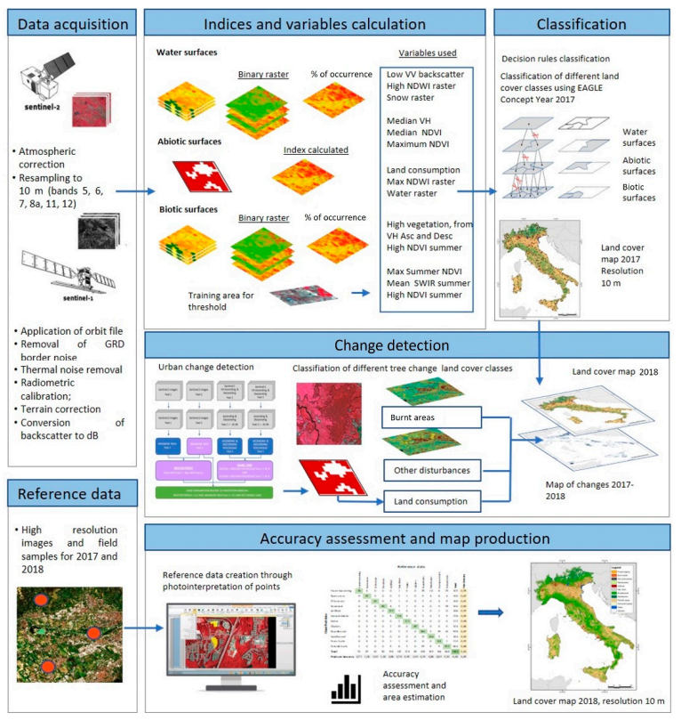
The methodology presented in this study uses Sentinel-1 GRD and Sentinel-2 images to map land cover and land cover changes in Italy, on a yearly basis (
Figure 1).
Decision rules are defined to identify land cover classes at pixel size of 10 m, setting fixed threshold values on composites (e.g., median, maximum) of multitemporal data. The rules are based on experience, on deep knowledge of literature and on previous analysis of temporal trend of spectral signatures, indexes and backscatter coefficients of each class. In this sense, the study is in continuity with other analysis published in previous scientific papers related with land consumption [
58,
59] and forest area monitoring [
18,
60]. Furthermore, the thresholds for vegetation classes were also defined using a collection of training areas. The output classifications were validated through the photo-interpretation of very high-resolution images.
The methodology was developed with Google Earth Engine (Javascript language program) but was also adapted for QGIS Semi-Automatic Classification Plugin and on a DIAS environment (ONDA
https://www.onda-dias.eu, accessed on 4 March 2021). This DIAS experimentation refers to the agreement between the Italian Space Agency (ASI) and ISPRA for habitat mapping.
2.2. Study Area
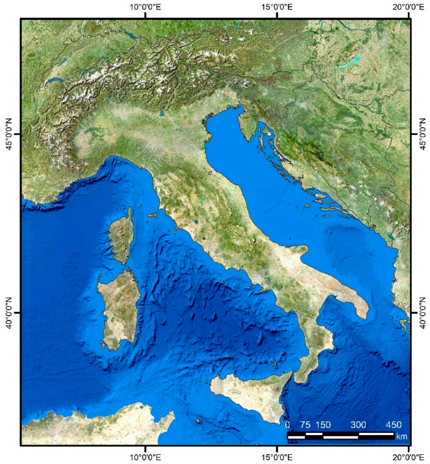
The study area is the Italian territory (
Figure 2), characterized by a total surface of 301,338 km
2. Geographically it is divided into three parts: The Alpine arc in the north, the peninsula in the south central part and the insular area that includes Sardinia and Sicily. The climate in the Italian territory is alpine in the north, continental in the peninsula and Mediterranean along the coast, with drier summers and milder winters. The average annual rainfall is higher in the mountain areas with a maximum of 2500–3500 mm and reaches a minimum of 500 mm in Apulia and Molise.
The territory is mainly composed of mountains (35.0%) or hills (41.6%) and plains (23.2%). The mountain belts are the northern area, forming the Alps with peaks reaching over 4000 m in the western part. The Appennines chain extends over the whole peninsula, reaching its highest peak with Gran Sasso (2912 m), located in Abruzzo. Due to these characteristics, the northern sector and the central chain are often covered by clouds or affected by perturbations that make it difficult to find cloud-free optical images for various periods of the year.
Land cover is characterized by forest, grassland, built-up areas and water (both liquid water and ice). Herbaceous vegetation is dominated by cropland and pastures and is mainly concentrated on coastal areas and, in Padana, plains. The orography conditions the distribution of the settlements, which are concentrated in the plains and on the coastal areas.
2.3. Classification System
The classification system defined for this research is consistent with the EAGLE group specifications [
32,
61] and it is composed of eight land cover classes, organized into three levels (
Table 1), and four land cover change classes (
Table 2).
The first classification level distinguishes three main land cover classes. It consists of land cover classes at the first two levels, while the “biotic-vegetated” class is then further articulated through a third classification level based on biophysical characteristics (broad-leaved, needle-laved) and temporal parameters (permanent herbaceous, temporary herbaceous).
- 1.
Abiotic-non vegetated: The class includes any unvegetated surfaces, either covered with man-made artificial structures or geologically natural material surfaces (with or without anthropogenic influence or impact). It includes consolidated or unconsolidated unvegetated natural surfaces, such as rocky regions and sands.
At the second classification level, the class is subdivided into artificial and natural surfaces.
- -
Artificial abiotic surfaces include impervious surfaces but also those of reversible land consumption [
62]. Impervious and sealed surfaces are mainly covered with features with a certain height above ground (artificial buildings and constructions) or features without a specific height above ground (flat waterproof surfaces) such as artificial surface pavements (e.g., asphalt, concrete, tarmacadam). Reversible land consumption includes all areas where natural surface material has been replaced by man-made material or where natural material has been removed, forming a non-impermeable and undeveloped surface. This includes soil compaction, excavation or temporary impervious cover. For example: unpaved roads, construction sites or courtyards or sports fields, permanent deposits of material, photovoltaic fields, and quarries not yet restored. The EAGLE classification system includes quarries and extraction sites in the 1.2.1.1 bare rock class, but in this research they are classified as artificial abiotic surfaces since quarries and extraction sites are strongly modified due to compaction and morphology changes caused by material removal. The physical characteristics of these areas are more similar to those of the EAGLE 1.1.2 “Non-Sealed Artificial Surfaces” class, which includes any open areas where natural surface material has been replaced by artificial material or where natural material has been removed from its place of origin as result of human activity forming an unsealed and non-built-up surface.
- -
Natural abiotic surfaces are any kind of surface material that remains in its natural consistence or form, either with or without anthropogenic influence. Consolidated and unconsolidated surfaces include: unvegetated rocky mountainous regions, sand, and bare soil.
- 2.
Biotic-vegetated: The class includes any terrestrial surface with spontaneous, semi-natural or artificial vegetation (e.g., crops and urban parks), with or without anthropogenic influence.
At the second classification level, biotic-vegetated surfaces are divided into woody vegetation and herbaceous vegetation.
- -
Woody vegetation includes perennial woody plants with a single, self-supporting main stem or trunk, containing woody tissue and branching into smaller branches and shoots.
A third classification level has been defined applying to the land cover class “trees” a characteristic related to the “leaf form”, allowing for distinguishing needle-leaved and broad-leaved trees.
- -
Herbaceous vegetation includes annual, biennial or perennial plants such as most ferns and grasses that do not have a persistent woody stem above ground. On the opposite to woody plants, the buds of herbaceous plants die at the end of the growing season, to regenerate from the tissues left above or below the ground (e.g., bulbs, rhizomes, tubers, seeds).
A third classification level has been defined applying to the land cover class “herbaceous vegetation”, a characteristic related to the “temporal parameter” of “duration”. In this way the class is divided on the basis of the persistence of the coverage throughout the year.
Permanent herbaceous areas are characterized by a continuous vegetation cover throughout a year. No bare soil occurs within a year. These areas are either unmanaged or extensively managed natural grasslands or permanently managed grasslands, or arable areas with a permanent vegetation cover or even set-aside land in agriculture.
Periodically herbaceous areas are characterized by at least one land cover change between bare soil and herbaceous vegetation within one year. Depending on the management intensities these areas can change between these two land cover components within a year. Normally these areas are arable areas.
- 3.
Water surfaces class includes water in its liquid or solid state of aggregation (snow and ice), both of natural formation (water basins, rivers, streams, stagnant waters, glaciers) and of artificial origin.
- -
Water bodies are water in a liquid state of aggregation regardless of location, shape, salinity and origin (natural or artificial). This includes all types of inland water surfaces without direct interference or interchange with open sea water, regardless of salinity and origin (natural or artificial). Watercourses (flowing water surfaces) come from: rivers, streams, canals, waterways. Stagnant waters (water surfaces of non-current waters, mainly lakes and ponds, or meanders of cut rivers) come from: natural lakes (both fresh and salt water), ponds, reservoirs, oxbow lakes, bottom pools, irrigation ponds, ponds for the production of artificial snow, river banks for the production of hydroelectric energy, and ponds for firefighting.
- -
Permanent snow and ice includes the snow cover that persists all year round, above the climatic snow limit and the persistent ice cover formed by the accumulation of snow.
The possible land cover change classes can be identified through a transformation matrix obtained starting from the considered land cover classes (
Table 3). This paper focused on the changes that can occur with a good probability within a year, between 2017 and 2018 (code 2 in
Table 3). These changes refer primarily to variations of artificial abiotic surfaces in terms of expansion (i.e., land consumption), reduction (i.e., restoration), and the loss of woody vegetation associated with forest disturbances (transformation from a woody vegetation class to natural abiotic surfaces or herbaceous vegetation). Code 1 of
Table 3 indicates changes that can be identified with good approximation by exploiting a series of multi-year images. The changes associated with these land cover classes have not been analysed in this paper, as the considered period is not wide enough to allow monitoring of transformations such as increases in woody vegetation increase or to distinguish seasonal variations from real changes in herbaceous classes. Finally, code 0 indicates transitions that are not within the objectives of the project.
A definition of the four land cover change classes analysed in this paper is provided below.
- 1.
Land consumption is the replacement of a non-artificial land cover to an artificial abiotic surface, both permanent and reversible. Artificial abiotic surfaces that have been changed by, or are under the influence of human activities resulting in a land consumption process can be sealed or unsealed.
- 2.
Restoration is the replacement of an artificial abiotic surface with a semi-natural land cover where permeable land is back, such as herbaceous (permanent and periodic), woody, or urban green.
- 3.
Forest disturbances are drastic decreases or disappearances of vegetation in areas classified as woody vegetation, not associated with land consumption. Forest disturbances are further distinguished into two classes, through the introduction of two elements relating to the status segment of the landscape characteristics of the EAGLE matrix.
- -
Burnt areas: The class includes natural woody vegetation affected by recent fires. This class includes recently burnt areas of forests, moors and heathlands, sclerophyllous vegetation, transitional forest-shrub formations, and areas with sparse vegetation.
- -
Other disturbances: The class “other disturbances” identifies the removal of all or most of the trees, large and small, on a surface, following a disturbance event other than a fire. Virtually all woody vegetation is removed from the site in preparation for the settlement of new wood or another class of biotic vegetation.
2.4. Pre-Processing of Images and Collection of Training Areas
Before the classification process, preliminary steps are required to collect training areas and preprocess the input images, in order to obtain the backscatter values for Sentinel-1 GRDs and reflectance values for Sentinel-2 images (
Figure 1).
Sentinel-2 L1C images were used in this study. The atmospheric disturbance affecting L1C pixels can increase the uncertainty of spectral signatures, therefore decreasing classification accuracy; however, Sentinel-2 L2A historical archive was not available at the time of research. The input images were cloud masked and pixels affected by clouds excluded from calculations. The cloud mask was made through a simple algorithm based on the quality assessment band as described in Google Earth Engine website (
https://developers.google.com/earth-engine/datasets/catalog/COPERNICUS_S2, accessed on 25 March 2021). It is worth highlighting that cloud mask products provided with Sentinel-2 images generally underestimate clouds [
63].
- -
application of orbit file;
- -
removal of GRD border noise (low intensity and invalid data);
- -
thermal noise removal to reduce discontinuities between sub-swaths;
- -
backscatter intensity calculation using radiometric calibration;
- -
terrain correction (orthorectification using the SRTM 30 m DEM);
- -
conversion of backscatter coefficient to dB; due to the wide dynamic range of SAR data, decibels were used to amplify the small variations and make the data more readable [
64].
The same preprocessing can be applied in the DIAS environment.
Sentinel-1 GRD and Sentinel-2 grids are not aligned and have different spatial resolution: in detail, the Sentinel-1 GRD have ground range geometry, and the pre-processing involves the geocoding to map coordinates. Sentinel-2 images are provided in WGS 84 UTM coordinates and cover the Italian territory with about 80 granules. In order to use both images in the same workflow, the spatial resampling to a common coordinate reference system and spatial resolution is required. In this study, Sentinel-1 data were aligned to the Sentinel-2 grid, in the WGS 84 UTM reference system.
Another preliminary operation is the photo-interpretation of 905 training areas. These are used for setting the thresholds in classifying woody vegetation and for the distinction between broad-leaved and needle leaved vegetation.
2.5. Classification Process
The production of the land cover map involves the calculation of multitemporal indices and decision rules that allows for the separation of land cover classes. The classification is pixel based: a pixel is assigned to a specific class if it has spectral and geometric characteristics that satisfy all the rules and thresholds defined for that class. The classification primarily regards the assignment to each pixel of one of the three classes at the first classification level (
Table 1). In detail, the water surfaces pixels were first identified. In the areas not classified as water surfaces, the presence of abiotic-non vegetated areas was evaluated, and finally the remaining pixels were attributed to the class of biotic-vegetated surfaces. This operation provides three masks, which are then further classified with reference to the second or third classification level, according to the methodology described below. For further details, please refer to
Appendix A.
Table 4 shows the spectral indices used for classification and calculations on the base of the Sentinel-2 images.
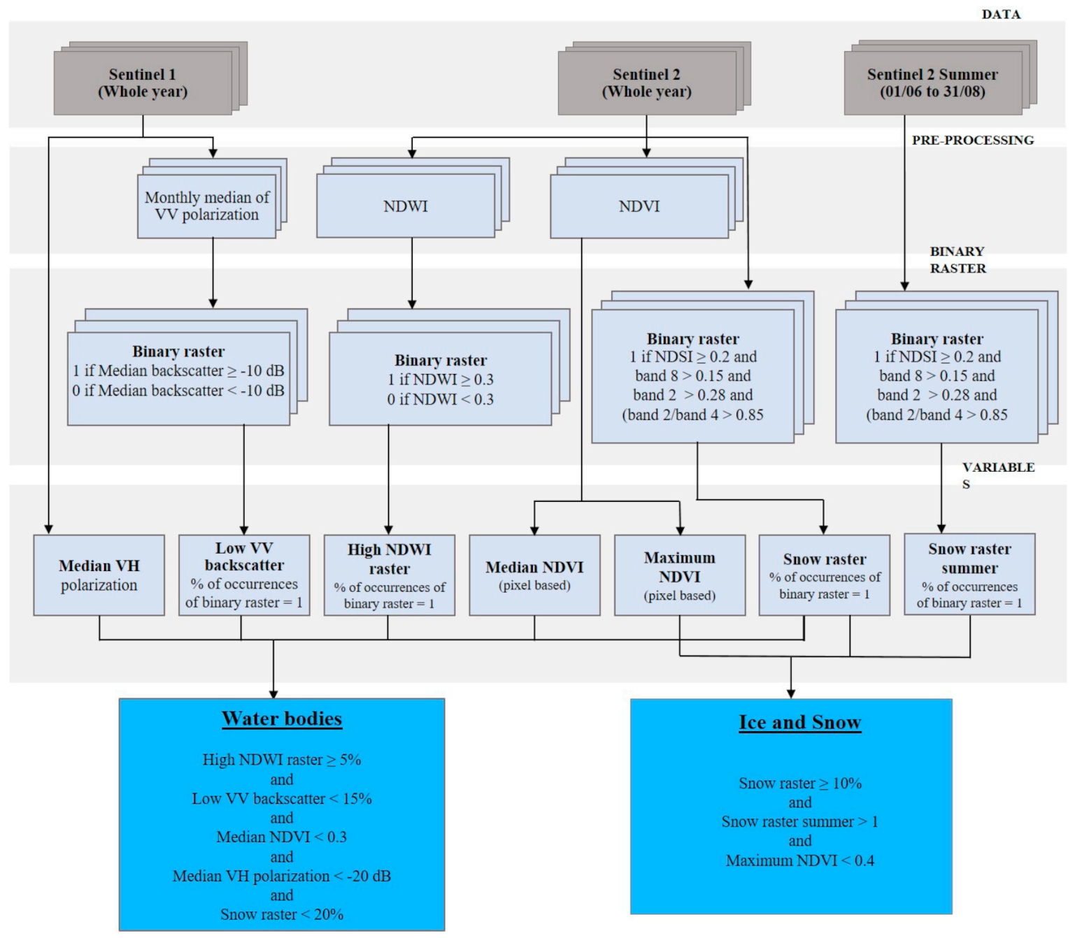
2.5.1. Water Surfaces
Water classes are required input for the classification of abiotic land cover classes; therefore, they must be classified before the others (
Figure A1).
Permanent Snow and Ice
The classification of permanent snow and ice is based on the definition of rules starting from the NDVI index and the “snow raster”. The “snow raster” derives from the methodology developed by ESA [
69] to detect snow surfaces, which are identified by pixels that have band reflectance lower than threshold values reported below:
and
and
and
The algorithm is based on the NDSI index, which exploits the property of snow surfaces to be very bright in the visible and dark in shortwave infrared bands (cloud and snow have similar reflectance in band 3 but band 11 reflectance for clouds is higher than snow). This index allows for the detection of snow and differentiating it from clouds, with values varying from −1 to 1. As a general rule, positive values define areas probably with a snow cover. The NDSI is flanked by three “filters” relating to band 8 (NIR), band 2 (blue) and the ratio between band 2 and 4. The thresholds are those indicated by ESA analysis. The snow raster represents the percentage of times that all the aforementioned conditions are satisfied during a specific reporting period.
The following three conditions are defined for the identification of permanent snow and ice.
- 1.
Snow raster ≥ 10%
The first condition to indicate the presence of permanent snow and ice in the pixel refers to the Sentinel-2 for the whole year. It defines that snow raster conditions must be verified in the pixel for at least 10% of valid observations. The threshold of 10% allows the elimination of outlier pixels.
- 2.
Snow raster summer > 1%
The second condition on the snow raster refers to Sentinel-2 images for the summer period (1 July–31 September) and a less conservative threshold of 1% has been adopted for the elimination of outliers.
- 3.
Maximum NDVI < 0.4
For each pixel, the maximum NDVI value is calculated with respect to the annual series of valid Sentinel-2 acquisitions. A threshold of 0.4 was defined to exclude areas with the presence of vegetation.
Water Bodies
Five conditions were considered in order to identify water bodies; each of them contributes to reduce possible mistakes between the spectral signature of water and other classes. Three rules are based on indices derived from Sentinel-2 images and two used Sentinel-1 GRD data sets.
- 1.
High NDWI raster ≥ 5%
It was observed by [
67] that water class has NDWI > 0 while non-water classes have NDWI < 0; a threshold value of 0.3 of NDWI was considered to better isolate water from the built up area and other surfaces [
70]. The first condition to indicate the presence of water bodies is based on NDWI values referring to Sentinel-2 for the whole year. It defines that NDWI ≥ 0.3 conditions must be verified in the pixel for at least 5% of valid observations. The threshold of 5% allows the elimination of outlier pixels.
- 2.
Median NDVI < 0.3
From the NDVI multi-temporal series for the whole year, the median of the NDVI for each pixel was calculated. A threshold of 0.3 was then defined in order to eliminate areas with vegetation.
- 3.
Snow raster < 20%
As for the class of perennial ice and snow, a “snow raster” was elaborated, relating to the annual Sentinel-2 series. The potential presence of water bodies was referred to pixels where snow raster conditions are verified in less than 20% of the annual valid observations.
- 4.
Median VH polarization < −20 dB
The backscatter values used in this classification are derived from tests carried out on sample areas and from values reported in the literature [
24,
71,
72]. The VH band discriminates quite well between the different classes presenting backscatter values around −20 dB, which remains constant throughout the year. Variations can be due to the wind, which makes the water surface rougher and modifies its backscatter. The potential presence of water bodies was referred to pixels with an annual median of the VH polarization < −20 dB.
- 5.
Low VV backscatter < −15%
The VV values are generally higher than VH ones. In the case of VV backscatter the value −10 dB was determined as a good threshold for identifying water [
24,
72]. A binary raster was produced starting from the monthly median (i.e., divided 12), attributing value 0 for values below −10 dB and 1 elsewhere. It was considered water class when the percentage of 1 throughout the year is less than 15%.
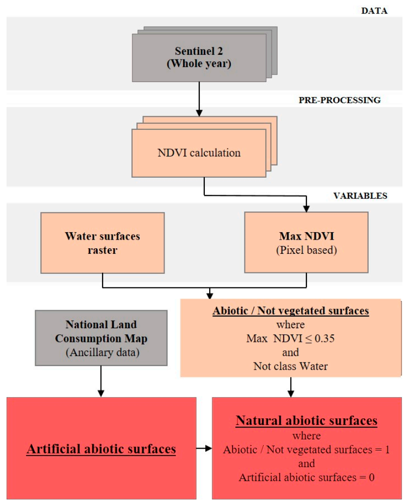
2.5.2. Abiotic Classes
The workflow for abiotic classes is based on the definition of two rules and requires only Sentinel-2 input images for the whole year. The abiotic surfaces are then distinguished between artificial and natural surfaces (
Figure A2).
- 1.
Maximum NDVI ≤ 0.35
A threshold of 0.35 is defined on the maximum annual NDVI value, in order to exclude areas that may present vegetation during the year. This calculation is in common with the processing of water classes; therefore, the same data were calculated only once.
- 2.
Not Water
Both the abiotic surface class and the water surfaces have low maximum NDVI values. To avoid commission errors, this second rule is defined, which excludes pixels previously classified as water surfaces.
Artificial Abiotic Surfaces
The distinction of natural and artificial abiotic classes is based on the National Land Consumption Map elaborated by ISPRA. The map was produced through supervied classification of RapidEye images using maximum likelihood algorithms [
73] and the methodology was then revised to use of Sentinel data. The map is updated every year through photointerpretation, with the help of masks of potential changes. The masks allow to reduce the area inspected by the photo interpreters, limiting the time and costs of the updating activity [
62]. This paper describes the results of the updating methodology, based on the use of Sentinel-1 and Sentinel-2 data; for details on the methodology for the production of the map, see Strollo et al. [
59] and ISPRA [
74].
Natural Abiotic Surfaces
Artificial surfaces and natural abiotic surfaces are very similar from a spectral point of view, so it is difficult to distinguish them only through the use of satellite images. The natural abiotic surfaces class has been identified considering the pixels classified at the first level as abiotic surfaces that have not already been classified as artificial abiotic surfaces.
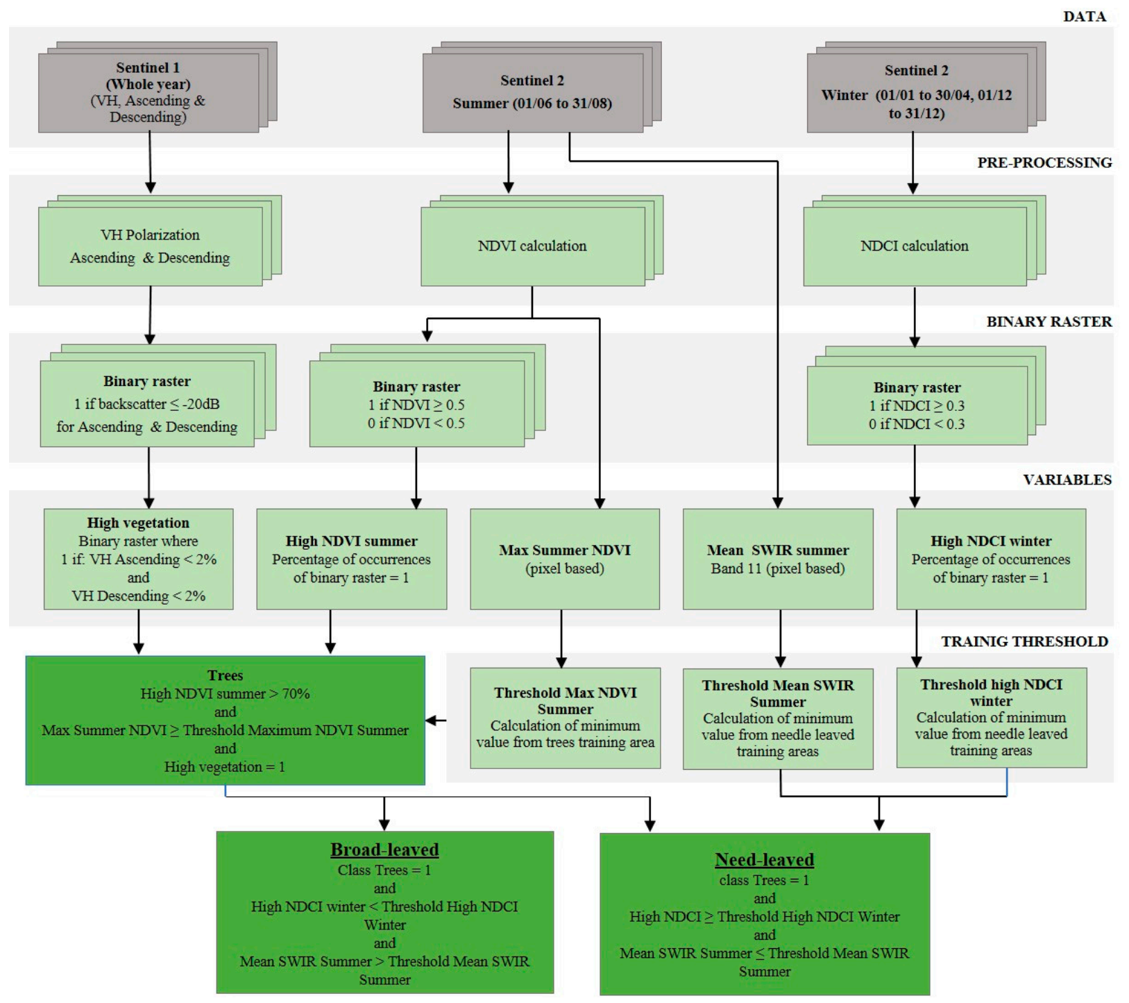
2.5.3. Biotic Classes
Biotic vegetation pixels are those that are not included in the classes of water and abiotic surfaces.
Woody vegetation was first identified and then divided into needle-leaved and broad-leaved trees. The land cover of the remaining areas was divided into periodically or permanent herbaceous, according to the EAGLE definition [
61].
The classification of biotic surfaces required the Sentinel-1 GRD dataset for the whole year and Sentinel-2 images for the whole year, for the summer period (1 June–31 August) and for the winter period (1 January–30 April and 1–31 December). Furthermore, 905 training areas were collected throughout the national territory, for the identification of the woody vegetation and for the distinction of needle-leaved and broad-leaved trees.
Woody Vegetation
Woody vegetation was identified through the definition of three rules. The first two rules are related to Sentinel-2 optical images, while the third is based on Sentinel-1 GRD data (
Figure A3).
- 1.
High NDVI summer ≥ 70%
The first condition to indicate the presence of woody vegetation is based on NDVI values referring to Sentinel-2 for the summer period (between 1 June to 31 August). It defines that NDVI ≥ 0.5 conditions must be verified in the pixel for at least 70% of the valid observations.
- 2.
Maximum NDVI summer ≥ Threshold on minimum value of the Maximum NDVI summer
The maximum NDVI value for the summer period (between 1 June to 31 August) was calculated for each pixel. This value was compared with a threshold obtained from the training area. In detail, the maximum summer NDVI was calculated in each pixel of the training areas and the lowest of them was taken as the reference threshold. Pixels with a maximum NDVI above the training area threshold are associated with the presence of woody vegetation.
- 3.
High vegetation
The backscatter of VH polarization for the whole year was used, as it can partially improve the detection between high vegetation (trees) and low vegetation (e.g., crops) [
75]. Since the acquisition orbit influences the angle of view, the ascending and descending orbits are considered separately. A conservative threshold of −20 dB has been defined for distinguishing low vegetation and fallow land (that generally have backscatter values lower than −11 dB [
76]), from trees (that generally have higher backscatter values). Pixels with backscatter values > −20 dB in at least 2% of valid observations, both for VH ascending and VH descending, were considered as woody vegetation. The 2% threshold is used to exclude possible outliers from time series of backscatter values.
Broad-Leaved and Needle-Leaved
Pixels classified as woody vegetation can be further distinguished in broad-leaved and needle-leaved using Sentinel-2 summer and winter images and training areas.
- 1.
Woody vegetation raster = 1
The conditions for distinguishing broad-leaved and needle-leaved are applied only to pixels classified as woody vegetation.
- 2.
Mean SWIR summer ≤ Threshold Mean SWIR summer (needle-leaved)
Mean SWIR summer > Threshold Mean SWIR summer (broad-leaved)
The spectral characteristics of needle-leaved and broad-leaved are very different in their wavelengths of short wave infrared (SWIR, band 11 of Sentinel-2 images). Starting from the training area of the needle-leaved pixels, the mean of the SWIR was calculated on the summer period (1 June–31 August) and the maximum value was set as a threshold. Needle-leaved pixels will have mean SWIR values for summer period lower than or equal to the threshold, while broad-leaved pixels will have higher.
- 3.
High NDCI winter > Threshold high NDCI winter (needle-leaved)
The third condition exploits a new empirical index developed in this research and called the “Normalized Difference Coniferous Index” (NDCI). The index is calculated on the winter subset of Sentinel-2 images (1 January–30 April and 1–31 December) and is the product of two normalized difference indexes: the first is based on band 6 (red edge, 740 nm) and band 12 (short wave infrared band, 2190 nm), and the second is based on band 8 (infrared, 842 nm) and band 11 (short wave infrared band, 1610 nm).
These bands show a more pronounced difference between needle-leaved and broad-leaved areas in winter than in summer. This is probably due to the drastic fall in the spectral response of broad-leaved trees compared to needle-leaved which do not drop their leaves in a senescence period [
44].
Starting from the needle-leaved training areas, the NDCI was calculated and a threshold of 0.3 was set. The percentage of times that NDCI > 0.3 in the winter period was then calculated for each pixel of the needle-leaved training area. The lowest of these percentages was set as a reference threshold for the distinction of needle-leaved and broad-leaved trees. Needle-leaved pixels will have frequencies of exceeding the threshold higher than or equal to the training area one, while broad-leaved will have lower.
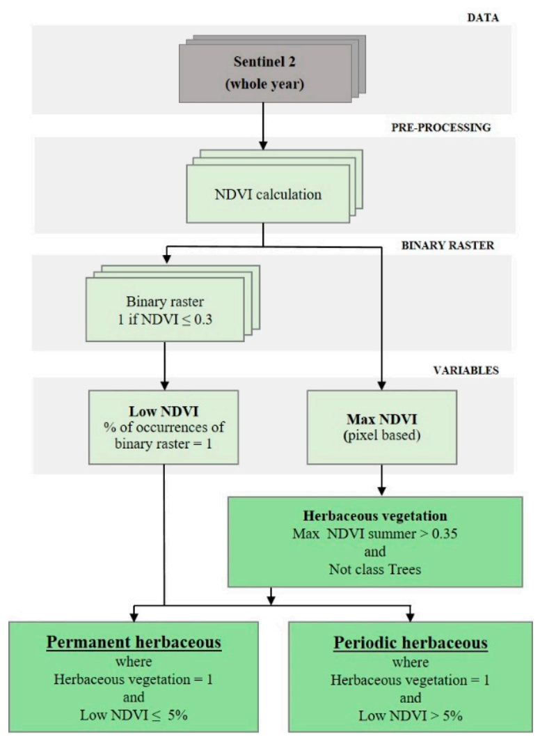
Herbaceous Vegetation
Herbaceous vegetation relates to pixels not previously assigned to other land cover classes (
Figure A4). These areas meet the following conditions:
As seen for the identification of abiotic surfaces, the condition distinguishes the vegetated areas from the unvegetated ones
- 2.
Not woody vegetation
Areas with vegetation cover but which do not respect the rules for falling into woody vegetation are considered herbaceous.
Permanent and Periodically Herbaceous
The pixels of herbaceous vegetation can be divided into permanent and periodically herbaceous, by defining conditions on the NDVI values calculated on the Sentinel-2 annual series:
- 1.
Low NDVI ≤ 5% (permanent herbaceous)
Low NDVI > 5% (periodically herbaceous)
Starting from the Sentinel-2 annual image series, the frequency with which NDVI < 0.35 (low NDVI) is calculated for each pixel. Pixels with NDVI values < 0.35 in less than 5% of valid observations have been classified as “permanent herbaceous”, since this condition implies a very constant presence of vegetation. Otherwise the pixel is classified as “periodically herbaceous”, since the vegetated cover was replaced by non-vegetated cover for several periods of the year. It is worth noticing that non-vegetated cover could also be snow cover.
2.6. Land Cover Changes
The algorithm allows the user to directly identify changes, through specific procedures, for the different change classes. This approach limits the propagation of errors that would occur if changes were sought by comparing two complete land cover classifications [
77]. The identification of changes of artificial abiotic surfaces involved the creation of masks of potential changes, used for the annual update of the National Land Consumption Map. In detail, Sentinel-1 and Sentinel-2 images for 2017 and 2018 were used. For Sentinel-1 data, thresholds on ascending and descending backscatter variations were defined, while for Sentinel-2 data thresholds regard the maximum NDVI value in the second year and the NDVI difference between the two years. Areas with high backscatter variations and/or strong reductions in NDVI between the two years were included in a raster of potential changes. The raster was used as a basis for the photo-interpretation activities, carried out for the updating of the National Land Consumption Map. The details of this study are described in another paper [
58].
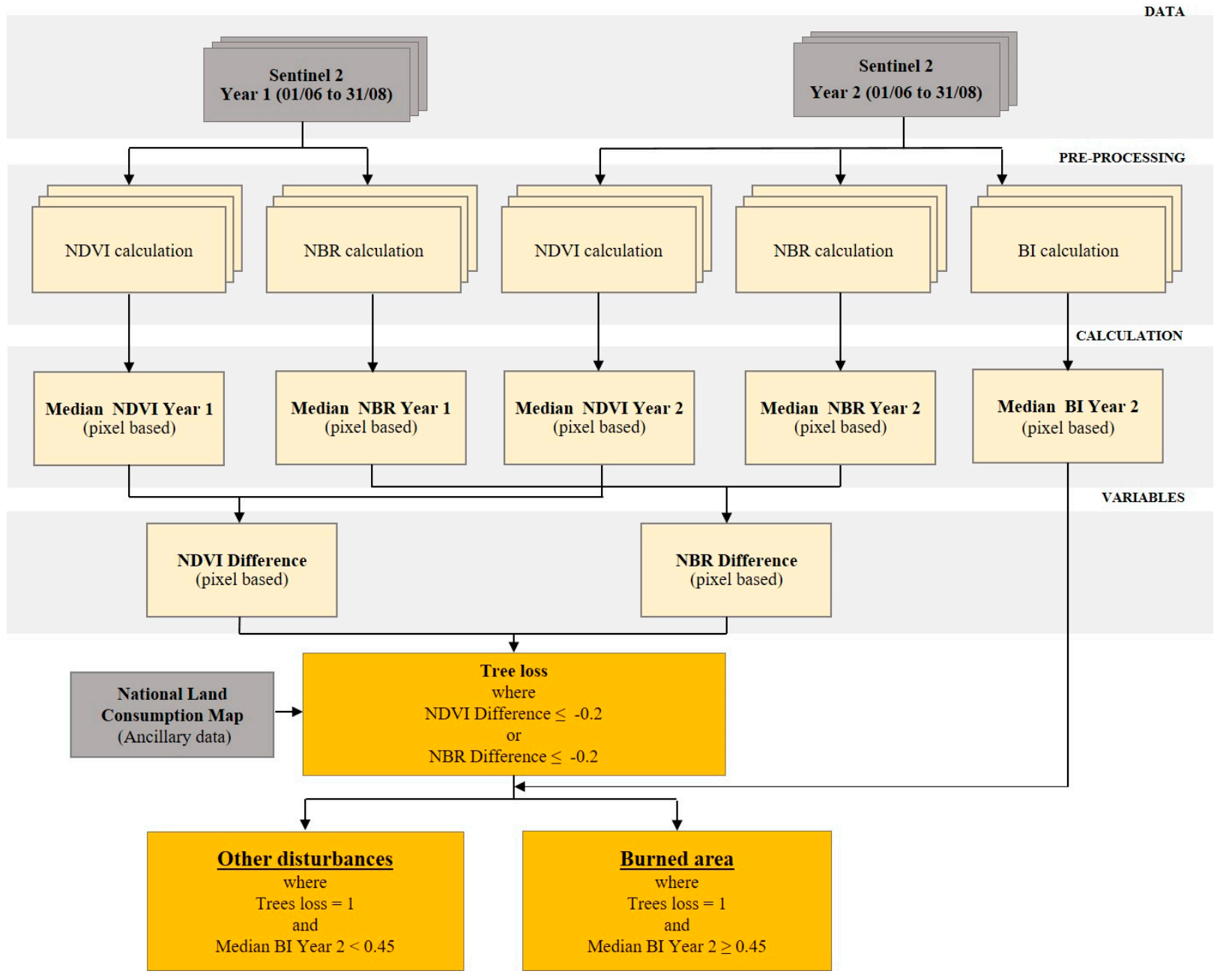
A specific methodology for mapping forest disturbance was developed, which also allows distinguishing burned areas from other kinds of changes such as forest harvesting (
Figure A5). The methodology is applied to areas classified as woody vegetation in the land cover map. This class acts as a mask for the delimitation of the forest area of year 1, within which the search for changes takes place. The input data used are the woody vegetation class for year 1 and the Sentinel-2 summer images (from 1 June to 31 August) for the two reference years. In this research, the changes that took place between 2017 and 2018 were analysed. Two spectral indices were calculated for the two reference years: NDVI and NBR [
78] (
Table 4).
NBR is useful for identifying areas that have been burned in the reference period. Notably, healthy vegetation has very high near-infrared reflectance and low reflectance in the shortwave infrared portion of the spectrum. Recently burned areas have a low reflectance in near infrared and a high reflectance in the short-wave infrared band.
NDVI is high in vegetated areas, while it decreases if there are reductions in vegetation cover.
To identify a forest disturbance, at least one of the following two conditions must be verified.
- 1.
NDVI Difference ≤ −0.2
The median of the summer NDVI is calculated for the two reference years and then the difference between the two values is considered:
If the difference is greater than 0.2, the change in NDVI indicates the presence of a change.
- 2.
NBR Difference ≤ −0.2
The difference between the median of the summer NBR of the two reference years is considered:
The threshold value 0.2 was identified empirically as optimal value for detecting tree loss and avoiding errors caused by phenological variations between years.
Distinction between “Burnt Areas” and “Other Distubances”
Starting from the pixels classified as forest disturbance, a distinction was made between “burned trees” and “other forest changes”, through an innovative burned index (BI) (
Table 4). The BI is higher for dark or brown pixels, as is in case of burned areas.
The median of BI of year 2 was calculated, obtaining a raster of “Median Burned Index Year 2”. Pixels already classified as forest disturbance can be further detailed in fires if Median BI Year 2 ≥ 0.45
The threshold value 0.45 was determined empirically as the optimal value for distinguishing burned areas and avoiding errors due to shadow areas where pixels tend to be dark.
2.7. Accuracy Assessment
The validation involved the 2018 land cover map with an eight-class classification system, integrated with the four land cover change classes.
First, a qualitative verification was carried out through a systematic visual search for macroscopic errors. An accuracy assessment on the base of Olofsson methodology was then performed [
79]; this approach is widely used in the literature [
79,
80,
81,
82].
The validation was carried out by identifying, ad hoc, a random sample of points which was then photo-interpreted using very high resolution images. The points were compared with the values of the land cover map at the same locations. The sample size (n) was calculated using the equation reported by Olofsson [
79] and referred to 5.25 in [
83].
where:
Wi—is area proportion of each classes derived from the map classification
Si—standard deviation of stratum
i,
Si = √(U
i(1−U
i)) ([
83], Eq. 5.55)
Ui—User accuracy of class i
S(Ô)—is the standard target standard error
Si influences the sample size, and its value is related to the Ui, which is unknown. A conservative scenario was assumed, considering Ui equal to 0.6 for all twelve classes.
The target standard error for overall accuracy was assumed to be 0.01 as suggested by Olofsson [
79], which corresponds to a confidence interval of 1%.
The application of (2) gives a sample of size 2400 (
Table 5).
The points were photo-interpreted with very high resolution images from Google Earth, considering 2018 as the reference year for the land cover classes and 2017 and 2018 for the land cover change classes. The photo-interpretation followed a pixel based approach, assigning to each point the class on which it falls exactly.
3. Results
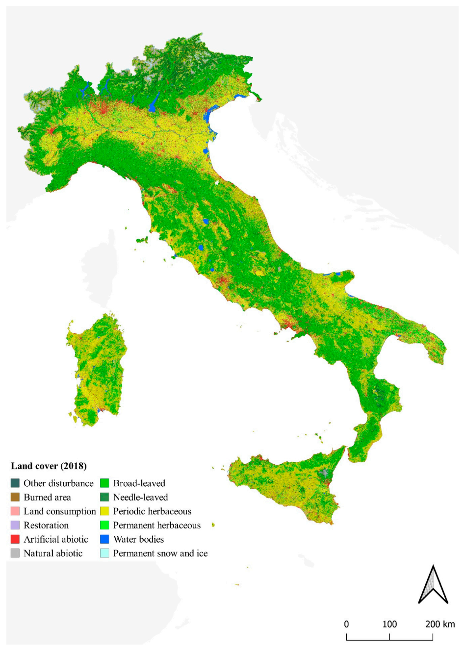
The land cover map shown in
Figure 3 was obtained from the application of the methodology. The map shows the eight land cover classes for 2018 and the four land cover change classes for 2017–2018 described above.
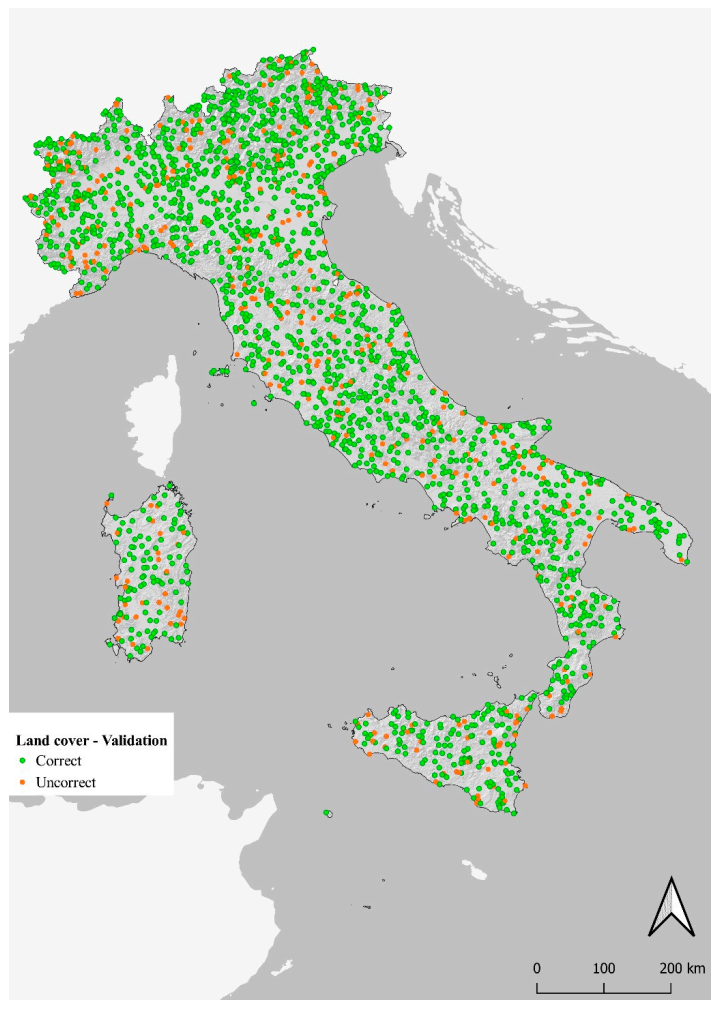
The map has 83% overall accuracy (
Table 7). This value offers a general estimation of the accuracy, but it is influenced by the distribution of the error between the classes, especially those of land cover change. This circumstance also affects the spatial distribution of the classification errors detected by the sample points of
Figure 4, since the land cover change classes do not have a specific distribution within the national territory.
Water bodies (98%), abiotic artificial surfaces (92%) and permanent herbaceous (92%) have the best user accuracy, while the land cover change classes show the lowest values, except for “land consumption” which presents a user accuracy of 81%.
As regarding the producer’s accuracy, four classes have values of 100%, and 9 out of 12 greater than 81%. The lowest values regard the land cover change class of “other disturbances” (71%) and the land cover class of permanent herbaceous (62%). Analysing the land cover data for 2018 and land cover change that occurred between 2017 and 2018 (
Table 8), 10.2% of the Italian territory is represented by abiotic surfaces, of which about 70% are artificial surfaces. The rest of the territory is divided between woody vegetation (45.2%, with a prevalence of broad-leaved trees) and herbaceous vegetation (42.8%, especially periodic herbaceous). The remaining 1.49% is represented by water bodies (1.1%) and perennial ice and snow (0.4%).
The four classes of change occupy 0.3% of the national territory and about 90% are forest disturbances.
Table 9 shows that between 2017 and 2018, land consumption (4231 hectares, i.e., 64.1% of total land consumption) and restoration (636 hectares, equal to 70.2% of restorations) occurred mainly in the periodically herbaceous class. The artificial abiotic surface is the class with more changes (both land consumption and restoration) compared to the class extension.
The decrease in vegetation caused by forest disturbances affects 89,596 hectares (
Table 10). 12.4% (11,106 ha) of forest disturbances are burnt areas, while 87.6% (78,490 ha) had other causes.
The “other disturbances” class was further analysed, showing that more than half of the disturbances are attributable to forest harvesting.
4. Discussion
The high overall accuracy of the map supports the rule-based classification method chosen, which allows the classification of the entire national territory with a relatively small number of training samples and frequent and fast updates of the map. Maxwell et al. and Thanh Noi et al. [
84,
85] assessed that the machine learning classification method achieves a high accuracy level; however, these methods are usually applied to limited areas, at a regional or local scale [
86,
87], or to a few land cover classes [
45,
88]. Moreover, as illustrated by Zhang et al. [
89], machine learning approaches such as random forest need to be trained with many samples, which must be balanced in order to avoid misclassification errors [
90], making the map update process slower.
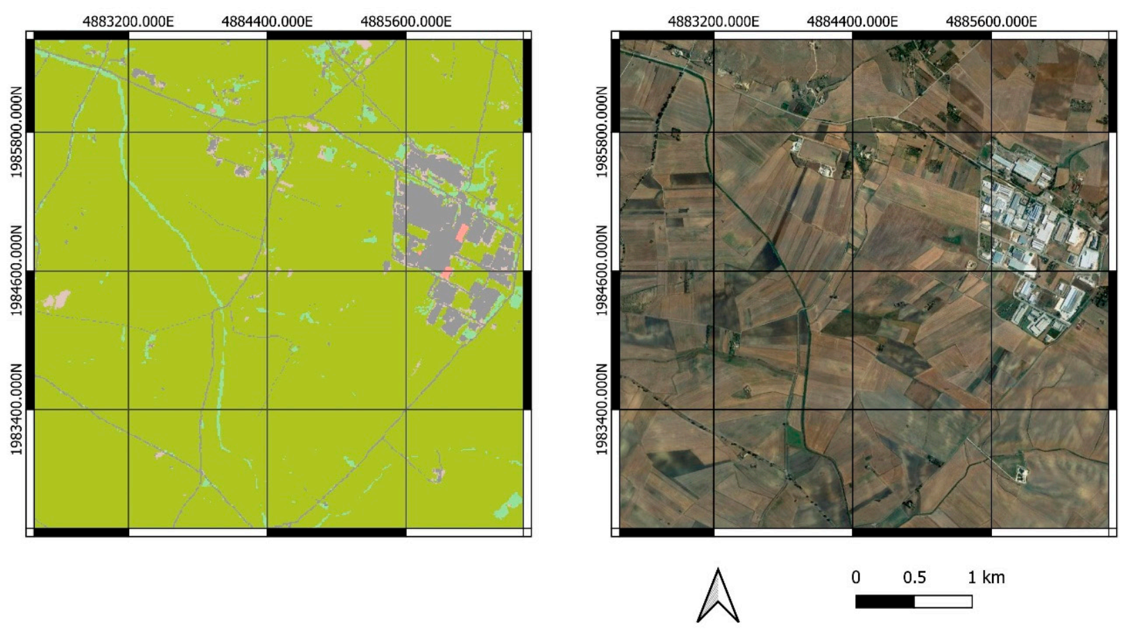
The developed methodology allowed for mapping the land cover and the changes in Italy, although with different results depending on the land cover class. The artificial abiotic surfaces and the changes related to land consumption were mapped using the National Land Consumption Map produced and updated by ISPRA. The use of ancillary data allowed for overcoming the issue related to spectral similarity between the natural abiotic surfaces and the artificial ones using Sentinel-2 images (
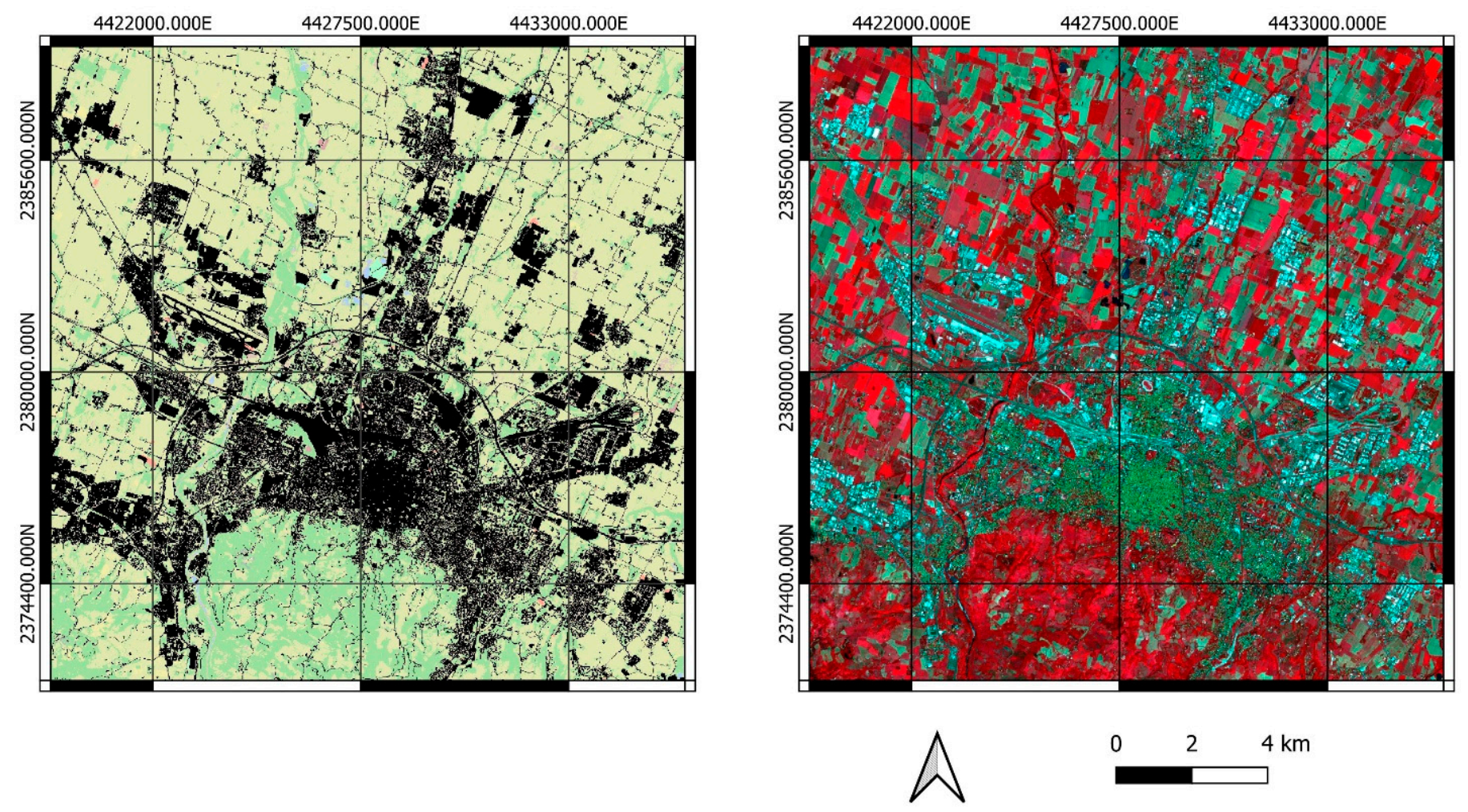
Figure 5). The data have high accuracy, due to periodic updates and improvements through photo-interpretation (
Figure 6). Hyperspectral images (such as PRISMA) could be used to improve the distinction of abiotic surfaces exploiting the bands in the SWIR region [
91].
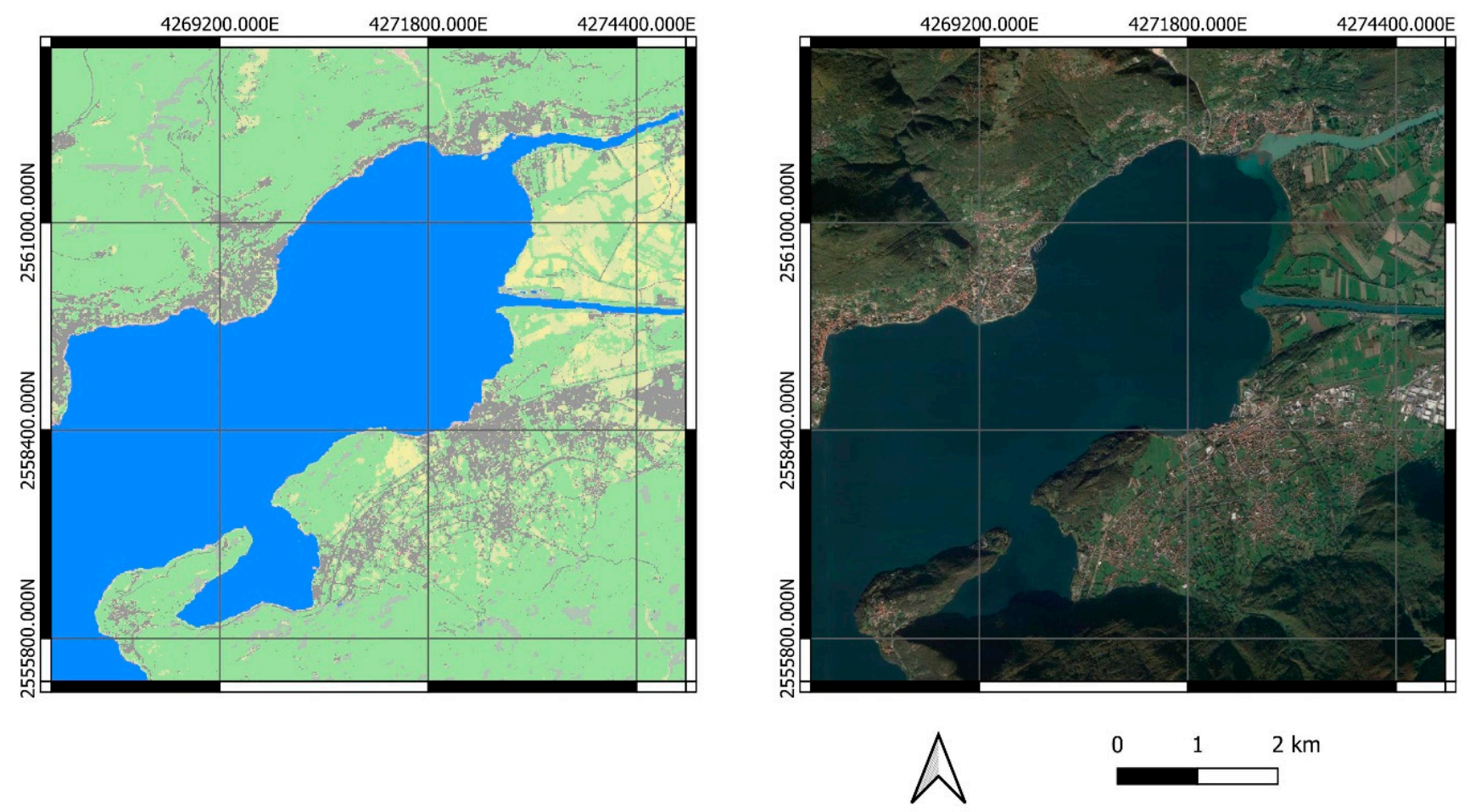
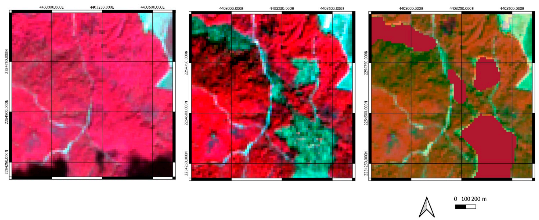
The class of permanent water bodies has an accuracy of over 90%, as the characteristics of the class can be well discriminated through the optical and radar instruments used in this research (
Figure 7). The few omission errors regard boundary areas between water bodies and other land cover classes, such as river and lake banks, and some wetlands.
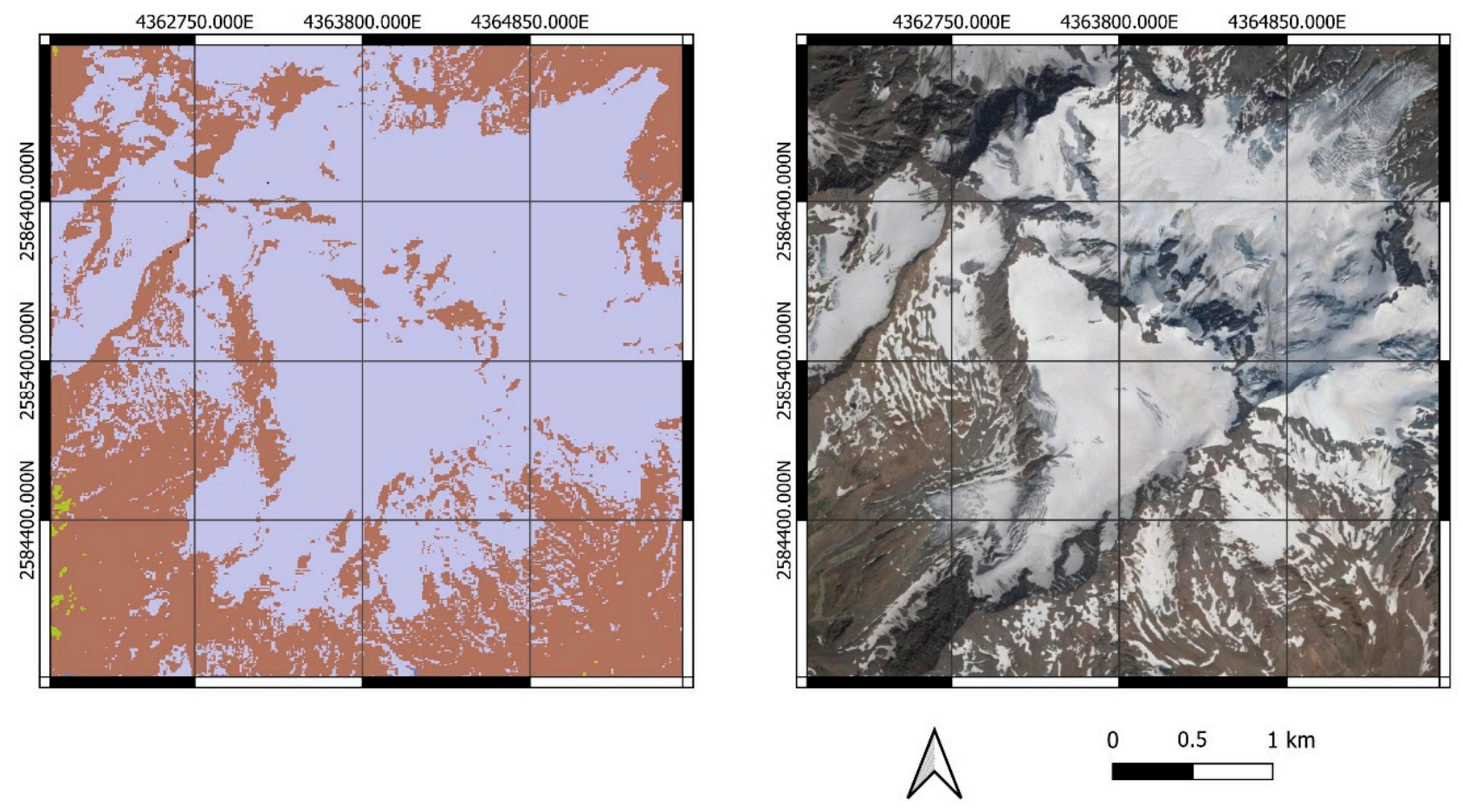
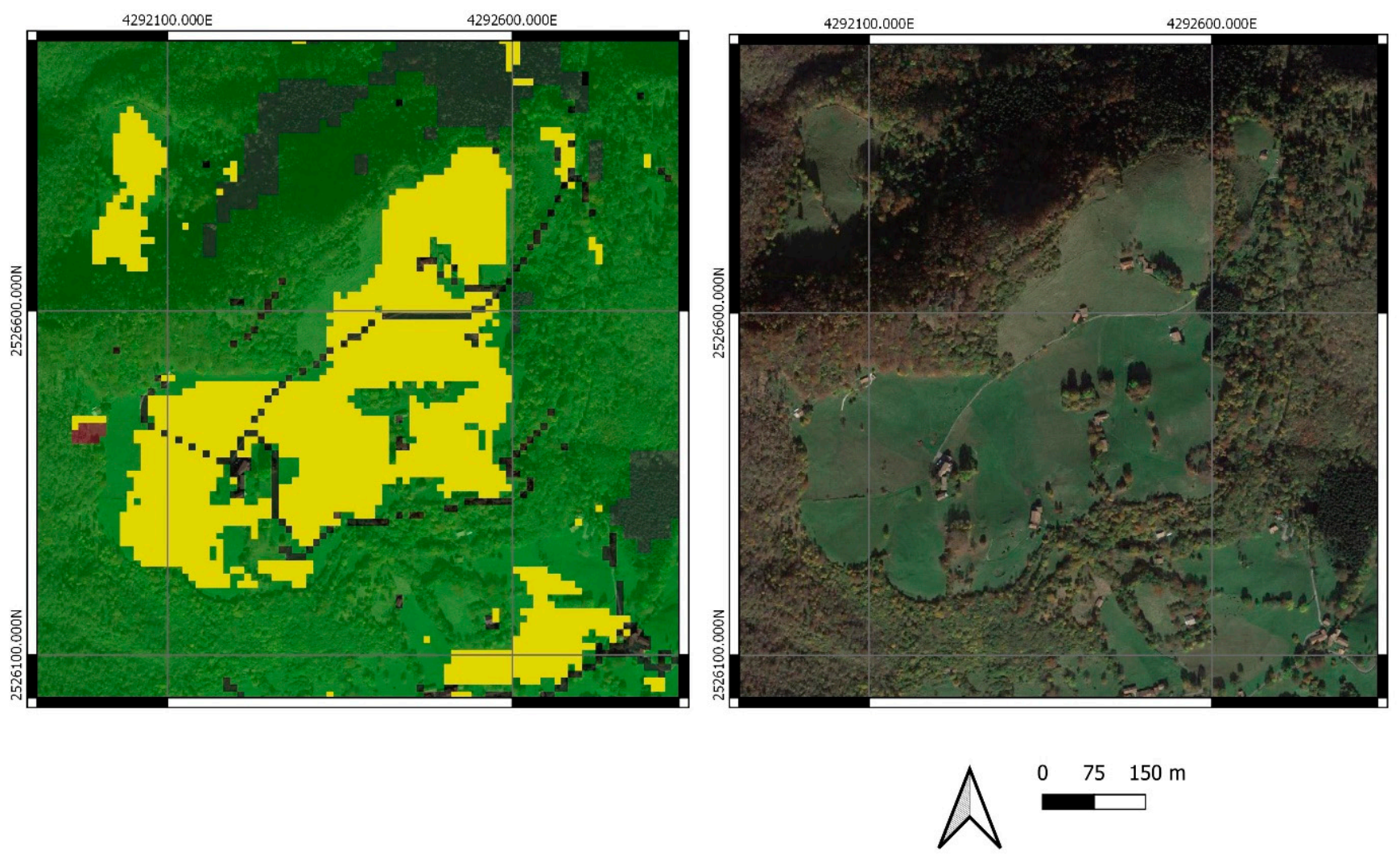
The class of permanent snow and ice has high accuracy (
Figure 8), although it is slightly lower than permanent water bodies (86%). The accuracy of the class is affected by commission errors related to the seasonal variation of snow cover.
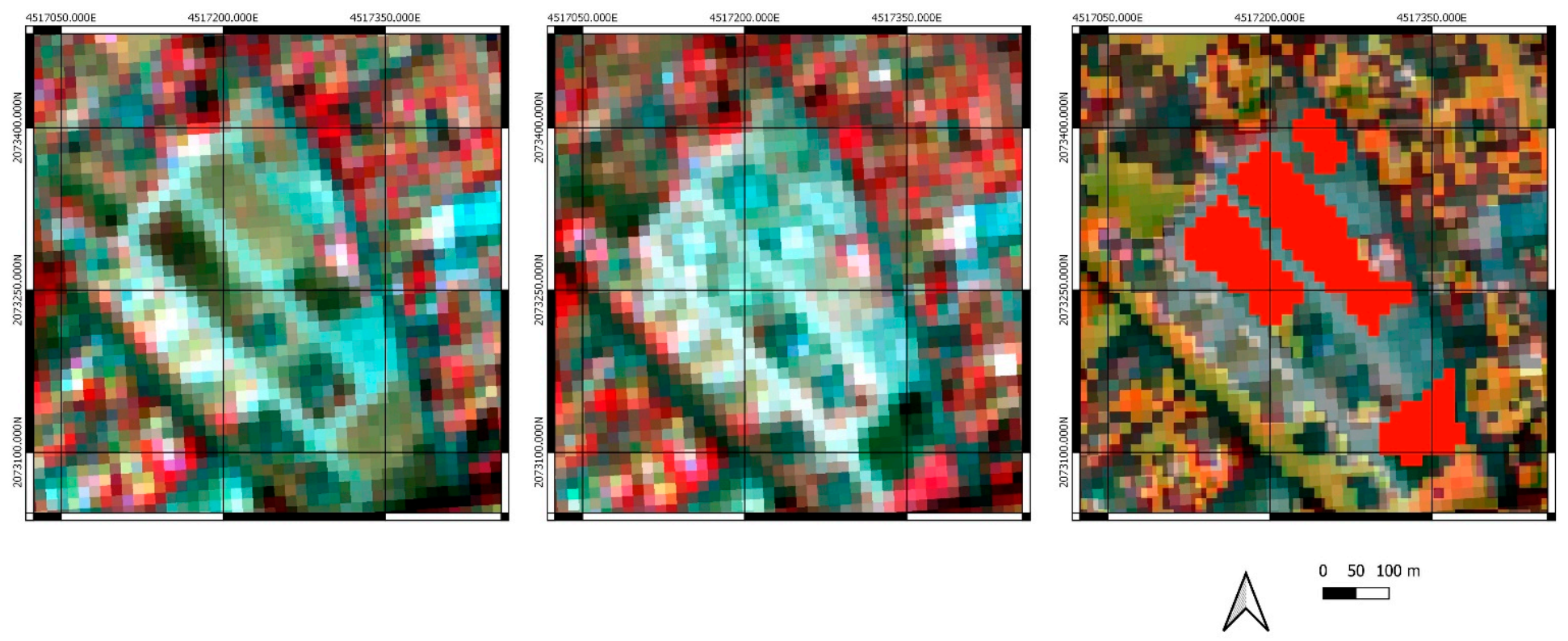
The classes of woody vegetation correctly distinguished between needle-leaved and broad-leaved trees in areas with homogeneous coverage, while in mixed forest pixels there are classification errors due to the spatial resolution of the data, causing mixed spectral signatures, and to the spectral similarity between the different types of trees (
Figure 9) [
6,
7,
92,
93].
The results obtained for the herbaceous cover are related with the definition of the classes of periodic (
Figure 10) and permanent (
Figure 11) herbaceous, which consider the persistence of the herbaceous cover in the pixel throughout the year. In detail, pixels showing herbaceous cover in at least 95% of valid observations were classified as permanent herbaceous. This threshold is conservative and aligned with the definitions of CLC+ products [
61], but it could be adapted to different temporal definitions.
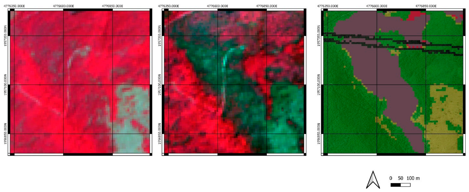
Forest disturbances (
Figure 12 and
Figure 13) are mainly affected by commission errors, due to the adoption of wide thresholds for the identification of the classes. Commissions are mainly related with permanent crops, since they have a spectral behavior similar to forest disturbances during the year.
The mapping of burned areas shows results aligned with the European Forest Fire Information System (EFFIS) (
https://effis.jrc.ec.europa.eu/, accessed on 25 February 2021).
The user accuracy of the class “other disturbances” is also low because it has been validated assimilating the class to “forest harvesting” only. The choice was made to evaluate the algorithm’s effectiveness in identifying this type of disturbance. Recently, several studies refer to the use of Sentinel data for monitoring forest disturbances, even if for limited areas [
94]. The size of the study area conditioned the identification of changes, since cuttings are conducted with different techniques which vary according to the geographical area; therefore, in some cases it is not possible to clearly associate the spectral variations to a certain type of disturbance. The detection of forest harvesting is more effective in Central Italy, while there are classification errors where selective logging method is practiced, such as on the Alps.
The observation of the areas of potential disturbance over a longer period can allow the improvement of the data [
60,
95].
The main objective of this research regards the formulation of a methodology that would allow the mapping and monitoring of land cover for the development of operational services, in compliance with the project requirements in terms of resolution, study area extension and update frequency. This paper presents a first product for 2018 that allowed the achievement of the project objectives and that actually lends itself to future refinements and improvements.
The EAGLE-based classification system allows for the introduction of new classes, such as shrubland, and can be modified for specific purposes, for example with land use attributes to identify agricultural activities in the herbaceous vegetation classes. The identification of shrubland will make possible a better description of Mediterranean macchia, permanent crops such as vineyards, transition areas and woodland boundaries. In this sense, it is necessary to conduct an in-depth analysis of the spectral behavior of shrubs, which are similar to scattered trees or to a mixed herbaceous and arboreal cover.
The use of Sentinel data constitutes an added value of the method, as they offer excellent results in the study of land cover at high spatial and temporal resolution, achieving high accuracy level with various classification algorithms [
57]. Furthermore, the free access policy also allows its use in contexts where financial resources for the acquisition of remotely sensed data are limited. Of course, additional classes would require additional methodologies, in the implementation of which the integration of hyperspectral data will be fundamental. The new HyperSpectral Precursor of the Application Mission (PRISMA) sensor, developed by the Italian Space Agency, has shown encouraging results in the distinction of forest types [
96]. This technology will be particularly useful with the launch of the “Hyperspectral Imaging Mission for the Environment” (CHIME) [
97], whose data will be freely accessible in the coming years.
A characteristic of the proposed method is the definition of thresholds and a set of rules which can be modified and adapted to different conditions. The use of a decision rules classification method has made it possible to develop ad-hoc rules for each land cover class, while the definition of fixed thresholds for the entire national territory makes the method easily controllable and implementable. On the other hand, the Italian territory presents a strong heterogeneity from the morphological and climatic points of view that cannot be neglected. In this sense, an important development of the methodology will regard the adaptation of the thresholds according to the characteristics of the territory, considering in the first place the influence of hydrometeorological variables and seasonal climatic variations on the indices. This topic is addressed by the working group in the publication by Spadoni et al. [
18], which involved a study area consisting of three Sentinel-2 granules and will be studied in depth. In this way it is possible to better analyse the phenological evolution of vegetation in order to improve the distinction between needle-leaved and broad-leaved trees and the identification of the different types of herbaceous classes and forest disturbances.
A further improvement regards the use of elevation models. At the moment this data has been used in the monitoring of changes associated with land consumption described by Luti et al. [
58] and will be able to guarantee important improvements in the land cover classification of mountain areas, especially in the shaded slopes of Alpine areas. In these areas it will be useful also to analyse the spatial correlation between pixels. This deepening can address the interpolation of missing or incomplete data [
98], enhancing some critical areas and allowing users to overcome classification errors due to input data characteristics (such as image shadows, or cloud coverage).
The versatility of the algorithm and of the classification system make the methodology suitable for future integrations and for adaptation for specific purposes, while remaining consistent with the requirements proposed at the national and European level.
5. Conclusions
The research has allowed the creation of a land cover classification methodology capable of providing nationwide products with high spatial resolution and accuracy. The methodology shows satisfactory results, allowing the achievement of all design requirements. It was conceived with the aim of obtaining products that can be used for operational purposes, with a high update frequency. Indeed, they fit well into the Mirror Copernicus initiative of the Space Economy Strategic Plan of the Italian Ministry of Economic Development, which provides for the creation of frequently updated products at a national scale, for the monitoring of the territory.
The approach based on decision rules guarantees the control of the choices adopted for the classification, and a high level of modularity. In this sense, the rules can be refined by inserting variable thresholds according to the characteristics of the area, such as latitude and phytoclimatic zone, hydrometeorological variables or elevation, but also they can be accompanied by other rules for the identification of additional classes. In this sense, the classification system based on EAGLE has an easily expandable structure, remaining consistent with the European indications in terms of classification systems. The methodology can be implemented quickly and easily and has a low computational cost, allowing the production of land cover maps that can be updated annually and with high spatial resolution.
The maps produced by the application of the methodology can also be used as ancillary data for the development of algorithms for monitoring and characterizing specific coverage classes, such as the detailed distinction of forest types, the characterization of agricultural areas or a more detailed analysis of forest disturbances. The methodology is therefore promising, thanks to the simplicity of the approach on which it is based and the ability to be applied to large areas while maintaining high spatial resolution and accuracy levels. In this sense, it is unique in the panorama of European and national land cover monitoring products.


 ,
, 


