Article

Identifying Urban Poverty Using High-Resolution Satellite Imagery and Machine Learning Approaches: Implications for Housing Inequality

1
School of Public Policy & Management, China University of Mining and Technology, Xuzhou 221116, China
2
School of Resource and Environmental Sciences, Wuhan University, Wuhan 430079, China
3
School of Urban Planning and Design, Shenzhen Graduate School, Peking University, Shenzhen 518055, China
4
Guangzhou Urban Planning & Design Survey Research Institute, Guangzhou 510060, China
*
Author to whom correspondence should be addressed.
Submission received: 7 May 2021 / Revised: 11 June 2021 / Accepted: 16 June 2021 / Published: 18 June 2021

Abstract

:
Enriching Asian perspectives on the rapid identification of urban poverty and its implications for housing inequality, this paper contributes empirical evidence about the utility of image features derived from high-resolution satellite imagery and machine learning approaches for identifying urban poverty in China at the community level. For the case of the Jiangxia District and Huangpi District of Wuhan, image features, including perimeter, line segment detector (LSD), Hough transform, gray-level cooccurrence matrix (GLCM), histogram of oriented gradients (HoG), and local binary patterns (LBP), are calculated, and four machine learning approaches and 25 variables are applied to identify urban poverty and relatively important variables. The results show that image features and machine learning approaches can be used to identify urban poverty with the best model performance with a coefficient of determination, R2, of 0.5341 and 0.5324 for Jiangxia and Huangpi, respectively, although some differences exist among the approaches and study areas. The importance of each variable differs for each approach and study area; however, the relatively important variables are similar. In particular, four variables achieved relatively satisfactory prediction results for all models and presented obvious differences in varying communities with different poverty levels. Housing inequality within low-income neighborhoods, which is a response to gaps in wealth, income, and housing affordability among social groups, is an important manifestation of urban poverty. Policy makers can implement these findings to rapidly identify urban poverty, and the findings have potential applications for addressing housing inequality and proving the rationality of urban planning for building a sustainable society.

1. Introduction

“End poverty in all its forms everywhere” was the first Sustainable Development Goal proposed by the United Nations in 2015. Poverty is a global problem that hinders sustainable development. Eradicating poverty is a global goal and one of the greatest challenges for developing countries. Measuring and monitoring poverty are essential for governments to help prevent poverty traps and promote resource reallocation. According to the poverty situation in middle-income countries, urban poverty has gradually become the main poverty problem associated with urbanization. For example, there were 244 million urban populations living on less than US $1.90 a day in China in 2015, according to the World Bank’s latest data. Urban and rural areas are interconnected organisms; thus, urban poverty research should be given the same attention as rural poverty research [1]. In particular, suburbs, as an important part of modern cities, have experienced a regional structural transformation from agriculture to manufacturing and services, and their population composition is diverse (e.g., landless farmers, intraurban residents, and immigrants) [2,3,4]. The social problems accompanied by rapid urbanization make suburban regions more vulnerable to poverty traps and regional inequality [5].
In recent decades, China has witnessed remarkable success in poverty reduction: the number of extremely poor was reduced by 646 million between 1993 and 2013 according to the World Bank’s statistical data [6]. However, poverty is still a serious problem in China based on new poverty characteristics [7]. One of the prominent features of poverty is that it has increasingly become urbanized. Since the reform and opening up of China in the 1980s, China’s economy has gradually moved from central planning to a market-oriented economy. During this period, China experienced rapid urbanization expansion, with an increase in over 39.45% of the urban population from 1978 to 2016, creating the world’s greatest population resettlement [8,9]. All population growth is expected to be absorbed by urban areas; however, some growth has occurred in less developed urban regions, and urban boundaries have extended beyond previous perimeters and into suburban areas [5]. Since the late 1990s, China has witnessed unprecedented suburbanization, with a large percentage of its population moving out of urban centers [10]. Subsequently, inner suburbs have been partly reconstructed, and with this increasing population, outer suburbs have attracted and activated local real estate development [11], which affects suburban development. Flourishing suburbanization has created inestimable socioeconomic benefits, especially improved residential housing conditions; however, this urbanization has also caused many problems, such as differentiation within urban low-income groups, problems caused by the development of suburban housing, and traffic jams, which increase suburban poverty and urban–suburban inequalities [5,12]. However, traditional poverty studies in China have focused on regional income inequality and rural poverty, and urban poverty was disregarded until the late 1990s [13,14]. Thus, with urbanization currently accelerating in China, it is worth focusing on raising the profile and enhancing our understanding of deprivation in urban contexts.
Urban poverty, as a comprehensive and complicated social phenomenon, has many indicators and dimensions for measurement [13,15]. Mapping and monitoring urban poverty have traditionally been conducted by household survey data or census data collected by National Bureau Statistics. These data are time consuming, expensive, and labor-intensive, which limits the ability to frequently and cyclically collect data in many areas. It is difficult to measure multidimensional urban poverty without focusing on the dimensions of living standards and housing conditions because they often reflect people’s consumption levels and basic economic situations [16,17,18]. Many scholars have explored the potential for using spatial, spectral, and textural features of built-up areas derived from high-resolution remote sensing imagery to measure urban poverty, which has been proven to be useful in monitoring local variations in poverty, especially when widely applied in exploring slum, informal, and formal settlements that are closely related to poverty [19,20,21,22,23,24,25,26,27]. These studies are mainly based on the premise that people who have similar demographic and social characteristics tend to cluster in neighborhoods with similar physical housing conditions. Remote sensing imagery, with the main advantages of higher frequencies, faster acquisition, and lower costs, has been increasingly utilized to explore urban poverty. For urban areas, different built-up areas share different unique sets of spatial and textural features (e.g., geometry, patterns, orientation, and spatial variability) that distinguish them from other areas [28]; therefore, local research is always needed.
Can the features of built-up areas extracted from remote sensing imagery be applied to rapidly explore urban poverty in China? There are many features that can be derived from imagery. Which features can be used to identify urban poverty in China, either in subsets or together? What do these features represent? To address these explorative questions, this study is organized as follows: After the introduction, Section 2 describes the study area, data source and processing, and methods. The experimental results are presented in Section 3 and discussed in Section 4. The last section summarizes this study and provides some implications.

2. Materials and Methods
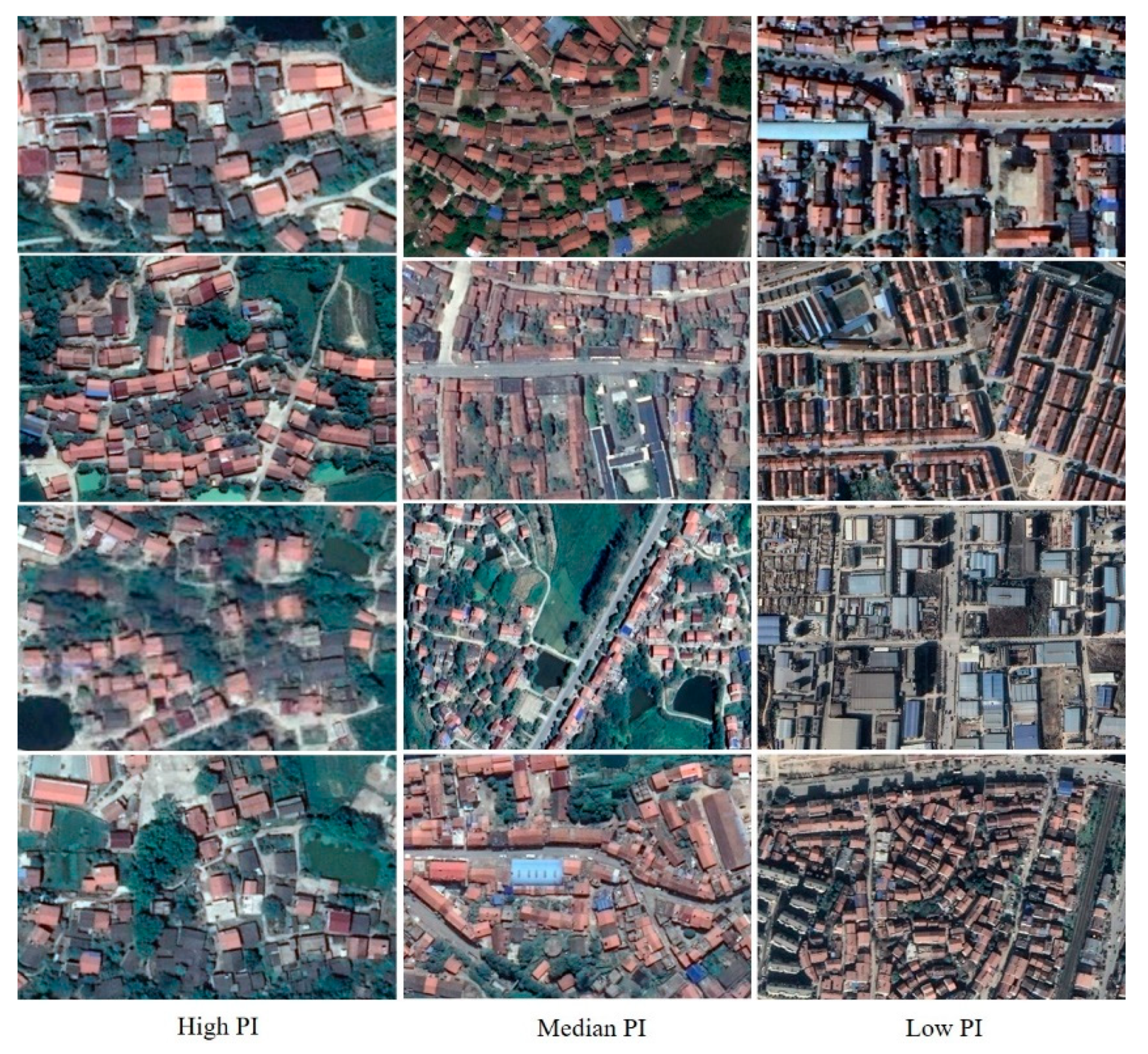
2.1. Study Areas

The case study areas are situated in the Jiangxia and Huangpi suburbs (Figure 1), which are located in Wuhan, China. Wuhan, the capital city of Hubei Province and the fast-growing metropolitan area with a strategic position in China, is situated in the eastern region of the Jianghan Plain at the intersection of the Yangzi River and Han River. Jiangxia, the southern gateway to Wuhan, is one of the six suburbs of Wuhan, with a total land area of 2018.3 km2 and a total resident population of 0.91 million in 2017. As an important connection and geographical location of the Wuhan metropolitan area, Jiangxia is experiencing an increasing population and urbanization rate. Huangpi, as the urban fringe of Wuhan, covers a total area of 2256.7 km2. Its regional gross domestic product (GDP) is approximately 70.25 billion Chinese yuan (CNY), with a total population of 1.13 million in 2017 and an urbanization rate of 45.52% in 2016.

2.2. Spatial Scale and Data Sources

This study assesses the relationship between urban poverty and the image features of built-up areas derived from remote sensing imagery at the lowest administrative level to ensure the relative homogeneity of regional built-up areas and efficient resource allocation by policy makers. The neighborhood committee or village committee, which is the lowest administrative level in China, serves urban communities. Influenced by the statistical unit of population data, some neighborhood/village committee units in Jiangxia have been split; thus, there are 408 spatial units in Jiangxia and 653 spatial units in Huangpi, which constitute the analytical region of this study.
The research data utilized in this study include the following data: (1) A collection of Google Earth (GE) imagery acquired in 2016, which contains 3 band multispectral (R: red wavelength, G: green wavelength, and B: blue wavelength) stacks with a 4.09 m spatial resolution, was applied to the analysis. GE imagery is an integration of satellite, aerial, and Street View images after data preprocessing; among them, the satellite imagery includes QuickBird, Landsat, and WorldView, and aerial data are mainly obtained from commercial companies. (2) A land cover dataset and boundary of administrative division from the Geographical Information Monitoring in 2016 was provided by the local department. (3) The 2016 population census and poor population statistics of neighborhood and village committees are sourced from the local department. All the datasets have geographic coordinate information, so we can combine them spatially. In this study, poverty incidence (PI) (proportion of poor to the regional total population) was selected to identify urban poverty, which is typically reported as one criterion to describe regional poverty.

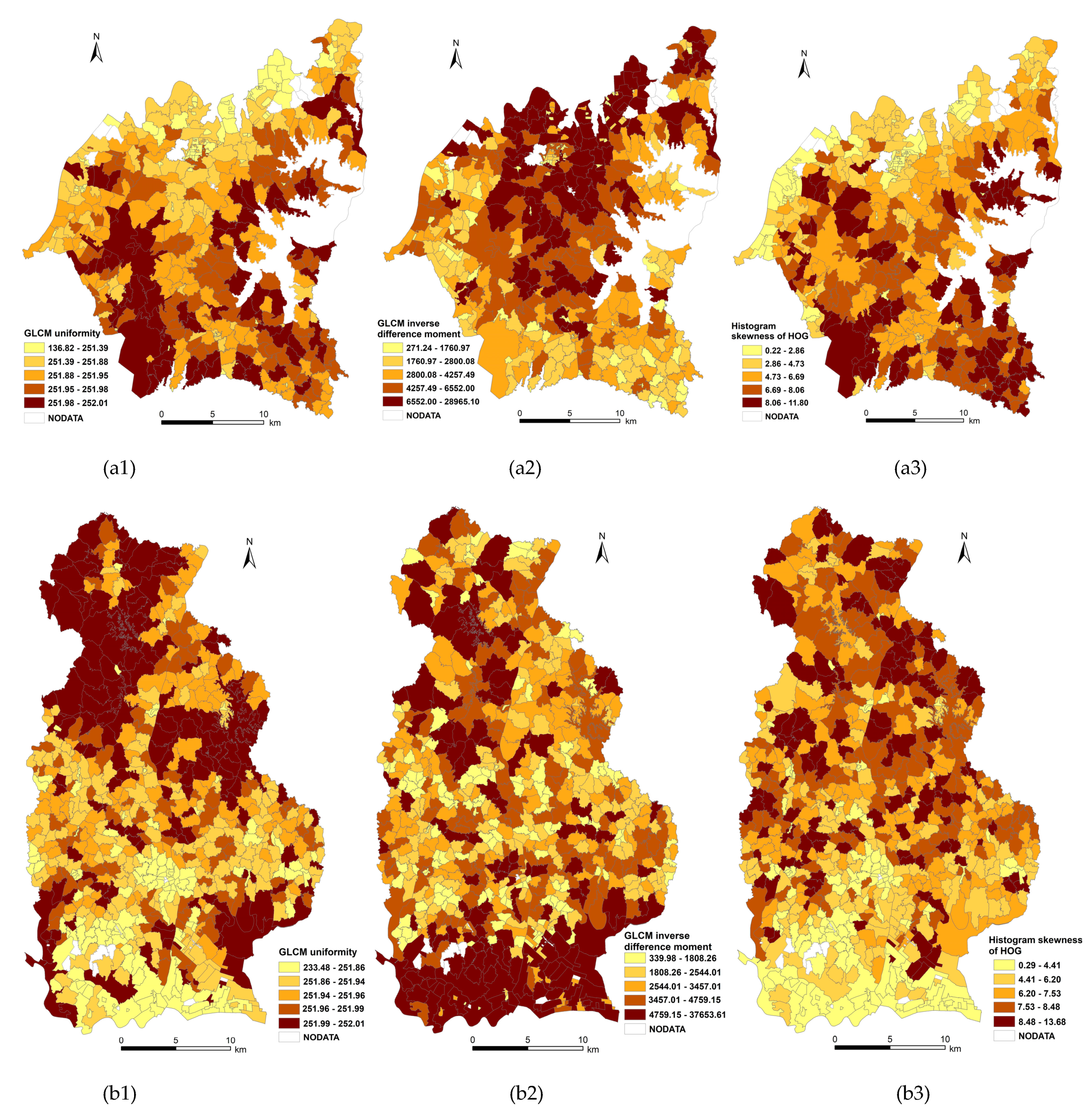
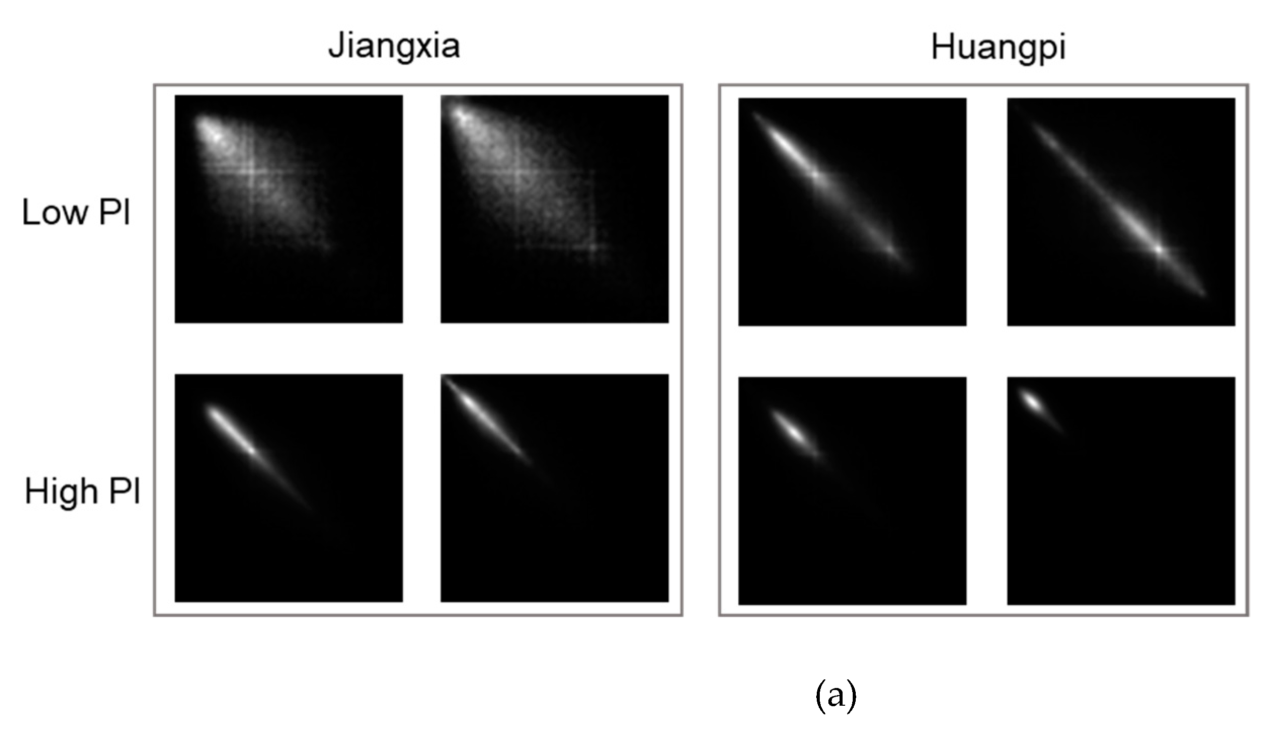
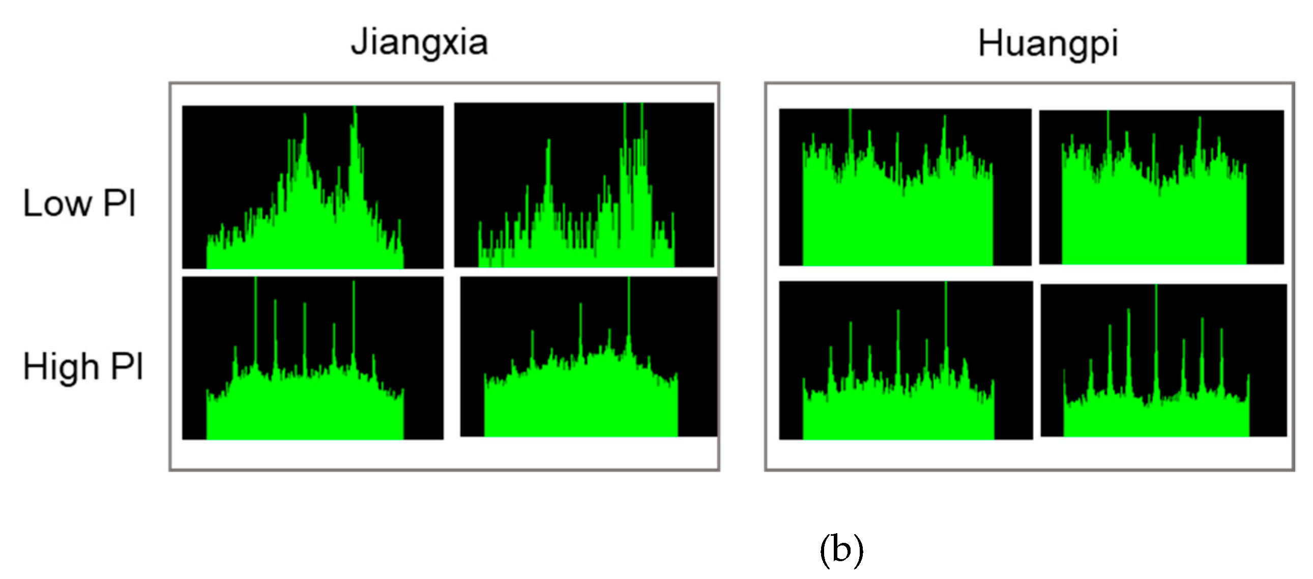
2.3. Calculation of Features

From the remote sensing perspective, image features such as geometric features, shape features, and texture features that are detectable and observable are variables with great potential to quantitatively distinguish the difference in built-up areas of committees with different poverty levels from the spatial patterning, texture, irregularity, and homogeneity of built-up layouts. Geometric features are constructed by a set of geometric elements such as lines, curves, or surfaces, which can be applied variables such as perimeter, orientation, and distance to differentiate objects. Shape features that are based on shape boundary information or boundary and interior content are the main basis of shape representation for describing the image content [29]. Reasonable shape descriptors, such as the line segment detector (LSD) [30] and Hough transform [31], can effectively distinguish similar shapes, although the database is affinely transformed. Textural features, which comprise an important low-level feature in the image, provide information about the spatial arrangement and distribution of the intensities or colors in an image. The gray-level co-occurrence matrix (GLCM) [32], histogram of oriented gradients (HoG) [33], and local binary patterns (LBP) [34] are significant measures that can be applied to quantify the perceived texture of an image by using texture features such as smoothness and coarseness.
To demonstrate the image features of built-up areas at the committee level, the six features calculated for this study were perimeter, LSD, Hough transform, GLCM, HoG, and LBP. Regional perimeters are especially useful in distinguishing simple or complex shapes. The simpler the shape is, the shorter the perimeter. The LSD aims to detect local straight contours on images, giving accurate subpixel-level results. The Hough transform is a measure for detecting curves based on the duality between points on a curve and the parameters of the curve. The GLCM is a typical method for describing image texture by exploring the cooccurrences of the pixel values, which is generally described by a set of textural variables, such as contrast, entropy, correlation, variance, inverse difference moment, and covariance. HoG, an edge and object detection method, captures the distribution of structure orientations [33]. LBP differentiates the forms of surfaces, edges, and corners and sorts them into a histogram [28]. Using the land cover dataset, the built-up area of imagery was obtained at the committee level. After processing, the built-up area of imagery and analytical region boundaries were employed to calculate the GLCM, Hough transform, and perimeter using the FETEX 2.0 software program [35], which is an interactive computer package that can be run in ENVI. LBP, HoG, and LSD were computed in Visual Studio 2017 using the Open Source Computer Vision Library (OpenCV), which is a cross-platform computer vision and machine learning library. Window size, a key parameter in image feature extraction, was chosen based on how many pixels the image feature calculation could differentiate in committees with different poverty levels in this study. Table 1 lists the variables that were included within the model to explore the relationship between the image features and urban poverty based on the variable selection procedure—the removal of variables that cannot be calculated for some committees or are unstable. In particular, random forests (RF), a technique for variable selection, can address instability and remove certain variables that do not significantly contribute to explaining results but can create random noise to prevent distinguishing the main effects [36]. Selected feature examples are shown in Figure 2. In particular, examples of screenshots of some features generated by FETEX 2.0 and OpenCV are presented in Figure 3.

2.4. Modeling Approaches

In an effort to explore whether features derived from remote sensing imagery are significant in differentiating urban poverty in China, 4 state-of-the-art machine learning regression approaches were selected in this research: Random Forest (RF), Gaussian Process Regression (GPR), Support Vector Regression (SVR), and Neural Network (NN). Machine learning approaches, which utilize example data or past experiences to optimize performance criteria to reflect nonlinear and complex relationships, have been increasingly applied to make predictions to guide or aid decision making [37]. As a branch of computer science, there are two major paradigms with machine learning approaches: regression and classification. Given that each approach has both merits and drawbacks, this study identified urban poverty by means of different regression models derived from the training data. In addition, two-thirds of the samples were selected for training, and the remainder were selected for validation.
Introduced by Breiman [38], RF is a regression or classifier model that consists of many regression trees, with each tree that is grown utilizing some form of randomization and with the same distribution for all trees in the dataset. This counterintuitive strategy performs better than many other classifiers and is robust against overfitting [39,40]. Originally developed as “kriging” in geostatistics, GPR is a nonparametric, nonlinear, Bayesian regression technique that is generally the most computationally demanding algorithm to train and that is useful in many fields because of its flexibility and expressiveness [41,42]. SVR, a kernel learning method, is based on the kernel technique for the distance-based optimization problem and linear approximation, which can achieve better accuracy and avoid computational complexity [43,44]. NN, an artificial neural network, is composed of artificial nodes or neurons, which can derive conclusions from a complex and weakly related set of information through self-learning from experiences that can occur within networks [45].
To select relatively important variables for identifying urban poverty, variable importance was calculated for all regression models used in this study. Variable importance quantification is an important procedure in pattern recognition, prediction, and phenomenon mining and for the interpretation of features and their effect on model accuracy [46,47]. The input variables for the different machine learning algorithms produce feature importance differences from one approach to another approach. In this study, the Mean Decrease Gini (MDG) and Permutation Accuracy Importance (PAI) are variable importance measures in RF, and the receiver operating characteristic curve (ROC) is applied to measure variable importance for GPR, SVR, and the NN. The MDG is the total decrease in node impurities measured by the Gini index and averaged over all trees. As the most advanced variable importance measure in an RF, PAI records the out-of-bag portion for each tree and after permuting each predictor feature. An ROC curve was created for each predictor, and the area under the curve (AUC) was calculated to measure variable importance. Relatively important variables are the independent variables needed for all the regression approaches in this study to achieve similar and better fitting results and are also important variables for identifying and explaining urban poverty. All modeling and variable importance for each regression model in this study were performed using the “caret”, “randomForest”, and “rpart” packages in R (version 3.5.2) and RStudio (version 1.1.463).

2.5. Model Performance Validation Method

The coefficient of determination (R2) was used in this study to quantify the model performance; it is defined in Equation (1).
R 2 = [ i = 1 n ( T i T ¯ ) ( P i P ¯ ) i = 1 n ( T i T ¯ ) 2 ( P i P ¯ ) 2 ] 2
where Ti, Pi, T ¯ , P ¯ , and n are the true values, predicted values, average true value at the ith analyzed unit, predicted PI value at the ith analyzed unit, and the number of analyzed units, respectively.

3. Results

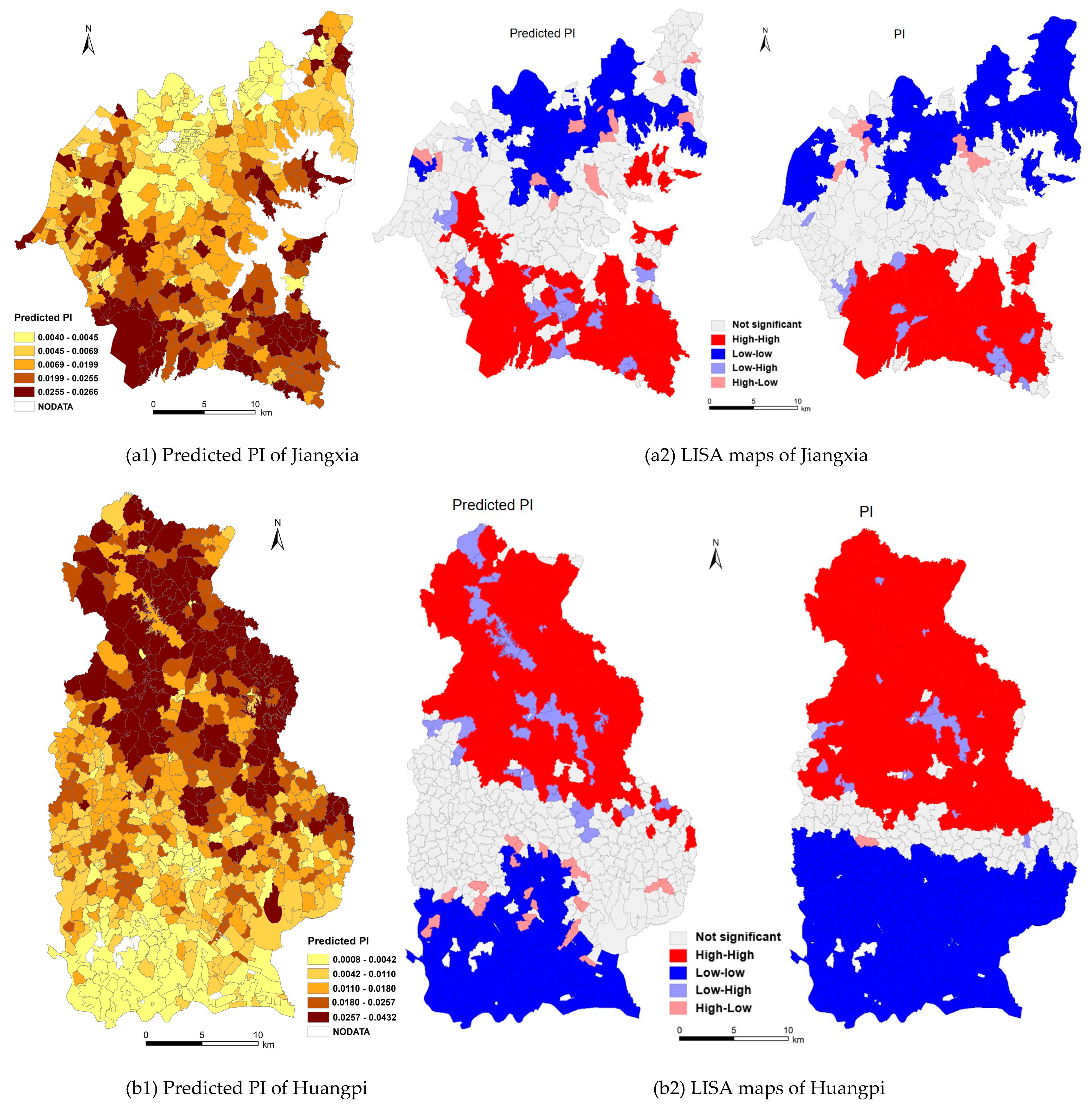
3.1. Model Performance

The best model performances are selected for each machine learning model by adjusting the parameters and number of sampling functions, which is defined as “set.seed” in the R software. Table 2 summarizes the model performances of the four models. The validation indicator of the regression results shows that the R2 that represents models’ performance of Jiangxia ranges from 0.3492 to 0.5341, and that of Huangpi ranges from 0.4231 to 0.5324. In particular, the results show that among the analyzed regressions, the SVR approach best presents the performance of Jiangxia and Huangpi, with R2 values of 0.5341 and 0.5324, respectively. It is concluded that in the best regression, features of built-up areas extracted from remote sensing imagery perform reasonably well independently for identifying urban poverty, exceeding 53% for explaining the poverty of Jiangxia and Huangpi. Compared to the prediction accuracy of Jiangxia, all of the algorithms, except for the SVR of Huangpi, generally present better model performances. Local indicator of spatial association (LISA) [48] is used to identify committees of concentrated poverty and to see if the predicted PI from remote sensing using NN can identify the same committees than the survey-based PI. Figure 4 shows a comparison of LISA maps of the predicted PI with the remote sensing-derived variables versus survey-based PI, which were both created using GeoDA. The maps show a general good match between the Low–Low and High–High committees, which means that the model fitted well throughout the Jiangxia and Huangpi rather than deviating toward high or low values. Although the model performance in this paper is general, it is acceptable for policy makers to rapidly determine which urban areas are poor.

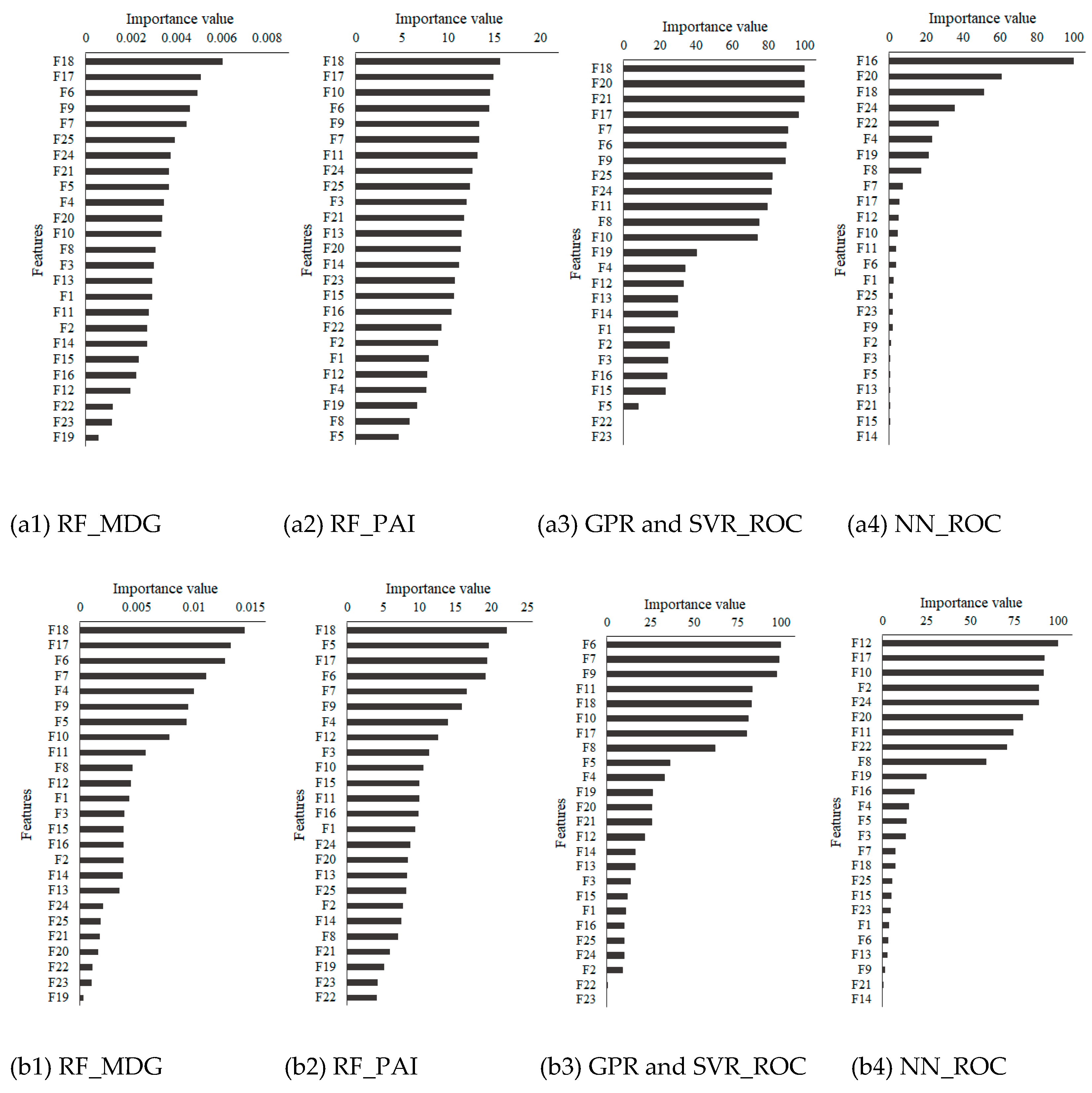
3.2. Important Variables for Identifying Urban Poverty

The relative importance of each variable for the applied machine learning models in this study is presented in Figure 5. The results show that the importance of each variable differs among the different models and study areas. In particular, the importance of each variable is similar when similar variable importance measures are employed for different models (e.g., GPR and SVR) and differs for the same approach (e.g., RF) when different variable importance measures are employed. Additionally, different study areas have a significant impact on the variable importance rankings. Although the importance of variables varies with models and study areas, the relatively important variables are similar and can be selected based on the frequency of occurrence in the order of variable importance. As shown in Figure 5, the variables that are relatively important for identifying urban poverty in the different machine learning models mainly include F18, F17, F7, F6, F9, and F10, representing the importance of GLCM and HoG for describing the characteristics of built-up areas with different poverty levels.
To better identify the variables that are most important for the regression results, we select several combinations of variables according to the frequency of each variable in the variable importance ranking for all models of Jiangxia and Huangpi to identify urban poverty. The model performance of the four models under five combinations of variables (4 variables: F18, F17, F7, and F6; 5 variables: F18, F17, F7, F6, and F9; 6 variables: F18, F17, F6, F7, F9, and F10; 10 variables: F18, F17, F6, F7, F9, F10, F11, F20, F24, and F5; 12 variables: F18, F17, F6, F7, F9, F10, F11, F24, F8, F4, F20, and F5) based on the proportion of variable importance of Jiangxia and Huangpi are summarized in Table 3. The results show that all models of Jiangxia and Huangpi with five combinations generally present relatively satisfactory prediction results, with R2 values that represent the models’ performance ranging from 0.2903 to 0.4793 and 0.3783 to 0.5189 for Jiangxia and Huangpi, respectively. Among them, the model performances for all models of Huangpi are mostly better than those of Jiangxia and vary among the five combinations. For the same model and study area, the five combinations have different model performances, and the best model performance does not correspond to the same combination. For example, the best model performance of NN in Jiangxia corresponds to four variables, while that of SVR corresponds to 10 variables. For different models and study areas, the model performance fluctuates with an increase in the number of variables, even achieving better results when there are four variables. Compared with Table 2, the results show that different models with different conditions can achieve better model performance, which is comparable to or even exceeds all variables included, indicating the effect of some important variables on the overall model performance. Although different models have different relatively important variables that guarantee better prediction results for each model, the top four variables (F18, F17, F7, and F6) achieved relatively satisfactory model performance for all of the models employed in this study, which indicates the importance of the four variables for identifying urban poverty in Wuhan city.
From Figure 5 and Table 2 and Table 3, the results show that a limited set of explicit features derived from imagery are sufficient for rapidly identifying urban poverty. In particular, F18, F17, F7, and F6 are the most relatively important variables in this paper, which suggests that textural features in terms of uniformity and entropy of pixels and kurtosis and skewness computed by a histogram should be considered more in similar future studies. Committees with positive HoG skewness and kurtosis represent a more uniform spatial layout, in which their buildings tend to be oriented homogeneously, as described in the histogram by most orientations falling into a minority of bins [25]. The uniformity and entropy demonstrate the complexity of committee texture features; specifically, the higher the value of entropy is, the more complex the gray distribution of the committee. To better understand the difference in important variables with lower and higher PI, the boxplots of F18, F17, F7, and F6 of Jiangxia and Huangpi are shown in Figure 6. From this figure, we can see that the four variables of Jiangxia and Huangpi present similar characteristics. For F18, F17, and F6, the variable value of relatively affluent committees is less than that of committees with a relatively low poverty level, while for F7, the characteristic is the opposite; that is, for Jiangxia and Huangpi, the layout of the less developed committees is more homogeneous, while the texture of built-up areas in the better developed committees is more complex. The well-developed committees are mostly mixed by residential land, commercial land, and industrial land, which makes the built-up areas of the committee quite different and heterogeneous. This phenomenon coincides with the current social situation in China, in which poor people are found to live in areas with a greater distance from social infrastructure. Thus, features calculated from high-resolution satellite imagery can be applied to study urban poverty, which has significance for rapidly monitoring and exploring regional poverty. Additionally, the application of those features can objectively reflect the rationality of urban planning, especially in China, with its rapid suburban development. In particular, the key to reducing suburban poverty is reasonable committee planning and developing a regional economy without increasing the problems caused by rapid suburbanization.

4. Discussion

Many scholars have proven that structural and textural features derived from remote sensing imagery that were applied to characterize the spatial pattern of the built-up layout are useful for slum index estimation and formal and informal identification [20,21,22]. Furthermore, some studies have evaluated the relationship between urban poverty or census-derived population characteristics and spatial and spectral features [19,28,49]. However, similar studies of Chinese cities are rare, especially studies in which only remote sensing imagery is employed. This gap in research may be attributed to a lack of obvious division among economic groups in China characterized by apparently different residential areas. Alternatively, this gap may be due to the lack of detailed urban poverty data and the focus on poverty alleviation in rural areas in China, which is determined by special national conditions. In an attempt to explore whether structural and textural features derived from high-resolution satellite imagery can be used to rapidly identify urban poverty in China, the better model performances of four machine learning approaches in two study areas provide a powerful response, which should demonstrate the exploration of urban poverty in China using remote sensing imagery that is objective and consistent. To further verify the relationship between structural features and textural features of built-up areas and urban poverty in China, we roughly divide the committees into three PI levels and compare the imagery of different levels of committees. Considering the limited imagery data source with an ultrahigh spatial resolution (0.26 m), Figure 7 presents some image captures showing areas of Jiangxia and Huangpi that have different levels of PI divided into three categories (high, median, and low) according to the PI value. The image captures are organized according to decreasing levels of PI from left to right to show the differences in the built-up area scenes as the level of PI decreases. From this figure, we can intuitively differentiate the spatial pattern of the urban layout of Jiangxia and Huangpi in terms of the settlement distribution on randomness or regularity, homogeneity or heterogeneity, and intensity and roughness as well as that of roads’ width, regularity, and type. Therefore, it is practical to identify urban poverty using structural and textural features from satellite imagery for Chinese cities. Since the settlement distribution is not the only aspect representing urban poverty, satellite imagery and machine learning approaches have shown the capacity to evaluate urban poverty at a reasonably high level of accuracy. Table 2 and Table 3 reveal the following phenomenon: the model performance of Jiangxia is generally lower than that of Huangpi, possibly because the PI of many committees in Jiangxia is 0 and Huangpi has more spatial units than Jiangxia, which inevitably affects model accuracy when it is sampled and calculated. In conclusion, the model performances from this study are acceptable, and it is feasible to rapidly explore urban poverty in China using high-resolution satellite imagery.
The results of the statistical analysis of this study indicate that the most important remote sensing predictors of urban poverty at the committee region level for Wuhan include histogram skewness (F18) and kurtosis (F17) of HOG, and entropy (F7) and uniformity (F6) of GLCM. These variables describe aspects of the spatial layout of buildings and the urban layout of texture features. Further analysis shows that the PI is higher in the analytical regions that registered higher homogeneity. However, there are some differences in the results compared to the findings of identification in favela, slum, and informal settlements or any other kind of urban poor area in other countries. In Medellin, the structural and texture descriptors indicate that a higher Slum Index registered higher overall complexity and lower variation in heterogeneity with distance [21]. The use of image texture measures for informal settlement identification has shown that these buildings have lower homogeneity and higher contrast. The authors of [20,22,24] found that the visual appearance and morphology of poor urban areas across the globe are very different, and the investigated areas showed a high spatiotemporal variability of morphological transformations. In particular, 13 cases indicated that the built-up structures led to a homogenous building alignment with decreasing complexity. These comparisons show that identifying urban poverty using satellite imagery for Chinese cities is needed. Further study is needed to determine how poor areas in Chinese cities have changed and the corresponding stages of transformation. Although high-resolution satellite imagery can be employed to identify urban poverty in China, the input remote sensing data are rather simple. Future research should address two main issues to improve existing models: (1) very high spatial resolution that can capture the differences in urban layout heterogeneity is needed; (2) additional datasets (e.g., Normalized Difference Vegetation Index, land cover classes, and nighttime light imagery) can be included to provide more details for poor urban areas in China.
However, this study also specifically found that although the model performance in identifying urban poverty using high spatial resolution imagery is often relatively satisfactory, the general variance that can be explained by those models often remains stable and not too high. Duque et al. [21] indicated that these variables derived from high spatial resolution image explain up to 59% in the Slum Index. In particular, Kraff et al. [24] revealed a high spatiotemporal variability of morphological transformations within studied areas, but the spatial patterns of building alignments remain predominantly constant. That is, identifying urban poverty using high spatial resolution imagery could provide a tendency and principal characteristics that cannot reflect all aspects of urban poverty. These results were expected. This may be explained by the multidimensional phenomenon in urban poverty, which involves many dimensions. The variables derived from high spatial resolution imagery reveal typical characteristics of the urban poor neighborhoods, which represent “morphological poverty”. Therefore, it is necessary to connect “ground survey data” obtained by in situ observations and interviews and “imagery variables” derived from high spatial resolution image to build valid and rigorous models. Only in this way a holistic and tangible reference for government decision makers is possible.
Housing is not only the basic space of urban activities, but it is also closely related to the social, economic, and spatial structure of a city. Poor people are found to live in areas of lower quality and densely populated neighborhoods, and the interior features of housing differ more widely between wealthier people and poor people [50]. There are many disadvantages of urban life for urban poor people of which housing is a prominent dimension [51]. The housing inequality pattern in China was formed before the country’s reform and still exists; housing consolidation has even occurred in recent years [52], while vulnerable groups contribute to experiencing housing difficulties. Thus, the rapid identification of urban poverty also reveals housing inequality. The significant spatial variation in urban poverty in Wuhan may be due to many geographic factors, including accessibility and proximity to various infrastructures, while housing inequality is more closely related to house prices and purchasing power. From a sustainability perspective, building economic housing in ideal urban areas where the poor can access basic services without excessive economic burden will not only contribute to social fairness but also help improve people’s livelihoods and well-being. It seems that the important variables for identifying urban poverty would be significant indicators for spatial analysis of housing inequality; disregarding geographic factors may fail to identify problems.

5. Conclusions

This paper seeks to identify urban poverty for one Chinese city solely using high-resolution satellite imagery at the community level. The usefulness of remote sensing data for estimating urban poverty was proven in the case of Jiangxia District and Huangpi District. Moreover, the variable importance of different models was used to identify relatively important variables for identifying urban poverty. The variables F18, F17, F7, and F6 achieved relatively good prediction results for all models, which indicates the importance of textural features for exploring urban poverty and deepens the understanding of the morphology of poor urban areas in China.
As an attempt at exploration for identifying Chinese urban poverty, this study confirms the validity of satellite imagery features, the existence of important variables, and implications for urban development and housing inequality. The findings can be applied to other cities as a directional and timely reference for policy makers to rapidly identify poor urban areas and provide assistance for renewal planning of poor communities. However, we should also have a clear understanding of the limitations of this study. First, restricted by data sources, we could only use relatively low-resolution imagery, and the study area did not include the main urban area of the city. Second, we only calculated a set of features and may have omitted other aspects. Third, data processing and the model performance of machine learning approaches should be improved in future studies. In future research, more detailed effects and applications of variables and methods of measurement can be applied to other cities with different social and environmental backgrounds.

Author Contributions

Conceptualization, G.L. and Z.C.; methodology, G.L. and Y.Q.; software, Y.Q.; validation, G.L., Z.C., Y.Q., and F.C.; writing—original draft preparation, G.L.; writing—review and editing, Z.C.; All authors have read and agreed to the published version of the manuscript.

Funding

This research was supported by “the Fundamental Research Funds for the Central Universities” [2021–11088].

Institutional Review Board Statement

Not applicable.

Informed Consent Statement

Not applicable.

Data Availability Statement

Not applicable.

Acknowledgments

We are grateful to the scholars whose work has inspired our own. Thank you to everyone who contributed to this study.

Conflicts of Interest

The authors declare no conflict of interest.

References

  1. Zhou, Y.; Liu, Y.S. The geography of poverty: Review and research prospects. J. Rural. Stud. 2019. [Google Scholar] [CrossRef]
  2. Christiaensen, L.; Todo, Y. Poverty Reduction during the Rural-Urban Transformation-the Role of the Missing Middle. World Dev. 2014, 63, 43–58. [Google Scholar] [CrossRef]
  3. Tang, S.S.; Pu, H.; Huang, X.J. Land Conversion and Urban Settlement Intentions of the Rural Population in China: A Case Study of Suburban Nanjing. Habitat. Int. 2016, 51, 149–158. [Google Scholar] [CrossRef]
  4. Sulemana, I.; Edward, N.A.; Emmanuel, A.C.; Jennifer, A.N.A. Urbanization and income inequality in Sub-Saharan Africa. Sustain. Cities Soc. 2019, 48, 1–8. [Google Scholar] [CrossRef]
  5. Xu, Y.; Zhang, X.L. The Residential Resettlement in Suburbs of Chinese Cities: A Case Study of Changsha. Cities 2017, 69, 46–55. [Google Scholar] [CrossRef]
  6. Chen, M.X.; Sui, Y.W.; Liu, W.D.; Liu, H.; Huang, Y.H. Urbanization Patterns and Poverty Reduction: A New Perspective to Explore the Countries along the Belt and Road. Habitat. Int. 2019, 84, 1–14. [Google Scholar] [CrossRef]
  7. Li, G.E.; Cai, Z.L.; Liu, X.J.; Liu, J.; Su, S.L. A Comparison of Machine Learning Approaches for Identifying High-Poverty Counties: Robust Features of DMSP/OLS Night-Time Light Imagery. Int. J. Remote. Sens. 2019, 40, 5716–5736. [Google Scholar] [CrossRef]
  8. Li, Y.H.; Jia, L.R.; Wu, W.H.; Yan, J.Y.; Liu, Y.S. Urbanization for Rural Sustainability--Rethinking China’s Urbanization Strategy. J. Clean. Prod. 2018, 178, 580–586. [Google Scholar] [CrossRef]
  9. Zeng, C.; Song, Y.; He, Q.S.; Liu, Y. Urban–rural income change: Influences of landscape pattern and administrative spatial spillover effect. Appl. Geogr. 2018, 97, 248–262. [Google Scholar] [CrossRef]
  10. Qin, H.; Liao, T.F. Labor Out-Migration and Agricultural Change in Rural China: A Systematic Review and Meta-Analysis. J. Rural. Stud. 2016, 47, 533–541. [Google Scholar] [CrossRef] [Green Version]
  11. Shi, Y.S.; Yu, Y.W. Whether Suburbanization Exacerbates or Alleviates Urban Diseases: Evidences from Shanghai, China. Econ. Geogr. 2016, 36, 47–54. [Google Scholar]
  12. Duque, J.C.; Royuela, V.; Noreña, M. A Stepwise Procedure to Determinate a Suitable Scale for the Spatial Delimitation of Urban Slums. In Defining the Spatial Scale in Modern Regional Analysis; Springer: Berlin/Heidelberg, Germany, 2012; pp. 237–254. [Google Scholar]
  13. He, S.J.; Liu, Y.T.; Wu, F.L.; Chris, W. Poverty Incidence and Concentration in Different Social Groups in Urban China, a Case Study of Nanjing. Cities 2008, 25, 121–132. [Google Scholar] [CrossRef]
  14. Chen, G.; Gu, C.L.; Wu, F.L. Urban Poverty in the Transitional Economy: A Case of Nanjing, China. Habitat. Int. 2006, 30, 1–26. [Google Scholar] [CrossRef]
  15. Appleton, S.; Song, L.; Xia, Q.J. Growing out of Poverty: Trends and Patterns of Urban Poverty in China 1988–2002. World Dev. 2010, 38, 665–678. [Google Scholar] [CrossRef] [Green Version]
  16. Panori, A.; Dimitris, B.; Psycharis, Y. SimAthens: A Spatial Microsimulation Approach to the Estimation and Analysis of Small Area Income Distributions and Poverty Rates in the City of Athens, Greece. Comput. Environ. Urban 2016, 63, 15–25. [Google Scholar] [CrossRef] [Green Version]
  17. Yuan, Y.; Xu, M.; Cao, X.Y.; Liu, S.J. Exploring Urban-Rural Disparity of the Multiple Deprivation Index in Guangzhou City from 2000 to 2010. Cities 2018, 79, 1–11. [Google Scholar] [CrossRef]
  18. Lucci, P.; Bhatkal, T.; Khan, K. Are We Underestimating Urban Poverty? World Dev. 2018, 103, 297–310. [Google Scholar] [CrossRef]
  19. Engstrom, R.; Newhouse, D.; Haldavanekar, V.; Copenhaver, A.; Hersh, J. Evaluating the Relationship between Spatial and Spectral Features Derived from High Spatial Resolution Satellite Data and Urban Poverty in Colombo, Sri Lanka. In Proceedings of the 2017 Joint Urban Remote Sensing Event (JURSE), Dubai, United Arab Emirates, 6–8 March 2017; Institute of Electrical and Electronics Engineers (IEEE): Piscataway, NJ, USA, 2017; pp. 1–4. [Google Scholar]
  20. Graesser, J.; Cheriyadat, A.; Vatsavai, R.R.; Chandola, V.; Long, J.; Bright, E. Image Based Characterization of Formal and Informal Neighborhoods in an Urban Landscape. IEEE J. Sel. Top. Appl. Earth Obs. Remote Sens. 2012, 5, 1164–1176. [Google Scholar] [CrossRef]
  21. Duque, J.C.; Patino, J.E.; Ruiz, L.A.; Pardo-Pascual, J.E. Measuring Intra-Urban Poverty Using Land Cover and Texture Metrics Derived from Remote Sensing Data. Landsc. Urban Plan. 2015, 135, 11–21. [Google Scholar] [CrossRef]
  22. Owen, K.K.; Wong, D.W. An Approach to Differentiate Informal Settlements Using Spectral, Texture, Geomorphology and Road Accessibility Metrics. Appl. Geogr. 2013, 38, 107–118. [Google Scholar] [CrossRef]
  23. Zhao, X.; Yu, B.; Liu, Y.; Chen, Z.; Li, Q.; Wang, C.; Wu, J. Estimation of poverty using random forest regression with multi-source data: A case study in Bangladesh. Remote Sens. 2019, 11, 375. [Google Scholar] [CrossRef] [Green Version]
  24. Kraff, N.J.; Wurm, M.; Taubenbck, H. The dynamics of poor urban areas—analyzing morphologic transformations across the globe using Earth observation data. Cities 2020, 107, 1–17. [Google Scholar] [CrossRef]
  25. Wang, J.; Kuffer, M.; Roy, D.; Pfeffer, K. Deprivation pockets through the lens of convolutional neural networks. Remote Sens. Environ. 2019, 234, 111448. [Google Scholar] [CrossRef]
  26. Wang, J.; Kuffer, M.; Pfeffer, K. The role of spatial heterogeneity in detecting urban slums. Comput. Environ. Urban Syst. 2019, 73, 95–107. [Google Scholar] [CrossRef]
  27. Müller, I.; Taubenbck, H.; Kuffer, M.; Wurm, M. Misperceptions of predominant slum locations? spatial analysis of slum locations in terms of topography based on earth observation data. Remote Sens. 2020, 12, 2474. [Google Scholar] [CrossRef]
  28. Sandborn, A.; Engstrom, R.N. Determining the Relationship between Census Data and Spatial Features Derived from High-Resolution Imagery in Accra, Ghana. IEEE J. Sel. Top. Appl. Earth Obs. Remote Sens. 2016, 9, 1970–1977. [Google Scholar] [CrossRef]
  29. Patel, M.N.; Tandel, P. A Survey on Feature Extraction Techniques for Shape Based Object Recognition. Int. J. Comput. Appl. T. 2016, 137, 16–20. [Google Scholar]
  30. Gioi, R.G.V.; Jakubowicz, J.; Morel, J.M.; Randall, G. LSD: A Fast Line Segment Detector with a False Detection Control. IEEE Trans. Pattern Anal. Mach. Intell. 2008, 32, 722–732. [Google Scholar] [CrossRef] [PubMed]
  31. Ballard, D.H. Generalizing the Hough Transform to Detect Arbitrary Shapes. Pattern. Recogn. 1981, 13, 111–122. [Google Scholar] [CrossRef] [Green Version]
  32. Baraldi, A.; Parmiggiani, F. An Investigation of the Textural Characteristics Associated with Gray Level Cooccurrence Matrix Statistical Parameters. IEEE Trans. Geosci. Remote Sens. 1995, 33, 293–304. [Google Scholar] [CrossRef]
  33. Dalal, N.; Triggs, B. Histograms of Oriented Gradients for Human Detection. In Proceedings of the IEEE Computer Society Conference on Computer Vision and Pattern Recognition (CVPR’05), San Diego, CA, USA, 20–25 June 2005; pp. 886–893. [Google Scholar]
  34. Ojala, T.; Pietikäinen, M.; Mäenpää, T. Multiresolution Gray-Scale and Rotation Invariant Texture Classification with Local Binary Patterns. IEEE Trans. Pattern Anal. Mach. Intell. 2002, 7, 971–987. [Google Scholar] [CrossRef]
  35. Ruiz, L.A.; Recio, J.A.; Fernández-Sarria, A.; Hermosilla, T. A Feature Extraction Software Tool for Agricultural Object-Based Image Analysis. Comput. Electron. Agric. 2011, 76, 284–296. [Google Scholar] [CrossRef] [Green Version]
  36. Sandri, M.; Zuccolotto, P. Variable Selection Using Random Forests. In Data Analysis, Classification and the Forward Search; Springer: Berlin/Heidelberg, Germany, 2006; pp. 263–270. [Google Scholar]
  37. Hu, L.R.; He, S.J.; Han, Z.X.; Xiao, H.; Su, S.L.; Weng, M.; Cai, Z.L. Monitoring Housing Rental Prices Based on Social Media: An Integrated Approach of Machine-Learning Algorithms and Hedonic Modeling to Inform Equitable Housing Policies. Land Use Policy 2019, 82, 657–673. [Google Scholar] [CrossRef]
  38. Breiman, L. Random Forests. Mach. Learn. 2001, 45, 5–32. [Google Scholar] [CrossRef] [Green Version]
  39. Liaw, A.; Wiener, M. Classification and Regression by RandomForest. R News 2002, 2, 18–22. [Google Scholar]
  40. Li, G.E.; Chang, L.Y.; Liu, X.J.; Su, S.L.; Cai, Z.L.; Huang, X.R.; Li, B.Z. Monitoring the Spatiotemporal Dynamics of Poor Counties in China: Implications for Global Sustainable Development Goals. J. Clean. Prod. 2019, 227, 392–404. [Google Scholar] [CrossRef]
  41. Cornejo, B.L.; Mateo, C.C.; Justo, J.S.; Sanz, S.S. Machine Learning Regressors for Solar Radiation Estimation from Satellite Data. Sol. Energy 2019, 183, 768–775. [Google Scholar] [CrossRef]
  42. Spradley, J.P.; Glazer, B.J.; Kay, R.F. Mammalian Faunas, Ecological Indices, and Machine-Learning Regression for the Purpose of Paleoenvironment Reconstruction in the Miocene of South America. Palaeogeogr. Palaeocl. 2019, 518, 155–171. [Google Scholar] [CrossRef]
  43. Cortes, C.; Vapnik, V. Support-Vector Networks. Mach. Learn. 1995, 20, 273–297. [Google Scholar] [CrossRef]
  44. Gonzalez, R.; Fiacchini, M.; Iagnemma, K. Slippage Prediction for Off-Road Mobile Robots via Machine Learning Regression and Proprioceptive Sensing. Robot. Auton. Syst. 2018, 105, 85–93. [Google Scholar] [CrossRef] [Green Version]
  45. Hopfield, J.J. Neural Networks and Physical Systems with Emergent Collective Computational Abilities. Proc. Natl. Acad. Sci. USA 1982, 79, 2554–2558. [Google Scholar] [CrossRef] [Green Version]
  46. Zeraatpisheh, M.; Ayoubi, S.; Jafari, A.; Tajik, S.; Finke, P. Digital Mapping of Soil Properties Using Multiple Machine Learning in a Semi-Arid Region, Central Iran. Geoderma 2019, 338, 445–452. [Google Scholar] [CrossRef]
  47. Strobl, C.; Boulesteix, A.L.; Zeileis, A.; Hothorn, T. Bias in Random Forest Variable Importance Measures: Illustrations, Sources and a Solution. BMC Bioinfor. 2007, 8, 25. [Google Scholar] [CrossRef] [PubMed] [Green Version]
  48. Anselin, L.; Syabri, I.; Kho, Y. GeoDa: An Introduction to Spatial Data Analysis. Geogr. Anal. 2006, 38, 5–22. [Google Scholar] [CrossRef]
  49. Niu, T.; Chen, Y.M.; Yuan, Y. Measuring urban poverty using multi-source data and a random forest algorithm: A case study in Guangzhou. Sustain. Cities Soc. 2020, 54, 102014. [Google Scholar] [CrossRef]
  50. Lejeune, Z.; Guillaume, X.; Marko, K. Housing quality as environmental inequality: The case of Wallonia, Belgium. J. Hous. Built. Environ. 2016, 31, 495–512. [Google Scholar] [CrossRef]
  51. Hu, L.R.; He, S.; Luo, Y.; Su, S.L.; Xin, J.; Weng, M. A social-media-based approach to assessing the effectiveness of equitable housing policy in mitigating education accessibility induced social inequalities in shanghai, China. Land Use Policy 2020, 94, 104513. [Google Scholar] [CrossRef]
  52. Zhou, Q.; Zhang, X.L.; Chen, J.; Zhang, Y.Y. Do double-edged swords cut both ways? Housing inequality and haze pollution in Chinese cities. Sci. Total Environ. 2020, 719, 137404. [Google Scholar] [CrossRef] [PubMed]
Figure 1. Study area map of Jiangxia and Huangpi with neighborhood and village boundaries.
Land 10 00648 g001
Figure 2. Selected feature examples showing the difference in feature of Jiangxia (a1a3) and Huangpi (b1b3) at the committee level.
Land 10 00648 g002
Figure 3. Examples of screenshots of some features generated by FETEX 2.0 and OpenCV: (a) gray-level image representation of the GLCM; (b) histogram image of HOG.
Land 10 00648 g003aLand 10 00648 g003b
Figure 4. Predicted PI (a1,b1) and LISA (a2,b2) maps of predicted PI with remote sensing-derived variables vs. survey-based PI of Jiangxia and Huangpi.
Land 10 00648 g004
Figure 5. Relative importance for the variables of different applied models in Jiangxia (a1a4) and Huangpi (b1b4).
Land 10 00648 g005
Figure 6. Boxplots of (a) F18, (b) F17, (c) F7, and (d) F6 of Jiangxia and Huangpi with lower and higher PI. The low PI of Jiangxia, high PI of Jiangxia, low PI of Huangpi, and high PI of Huangpi are represented as J_Low, J_High, H_Low, and H_High, respectively.
Land 10 00648 g006
Figure 7. Image captures from high-resolution satellite imagery (0.26 m) showing suburban areas that have different levels of PI.
Land 10 00648 g007
Table 1. Variables derived from remote sensing imagery.
Image FeatureMeasureVariableDescriptionAbbreviation
Geometric featuresPERIMETERPERPerimeter of each object F1
Shape featuresLSDLSD_TotNumTotal number of linesF2
LSD_TotLenTotal line lengthF3
LSD_MeanLenMean line lengthF4
LSD_VarLine varianceF5
Texture featuresGLCMUNIFORGLCM uniformityF6
ENTROPGLCM entropyF7
CONTRASGLCM contrastF8
IDMGLCM inverse difference momentF9
COVARGLCM covarianceF10
VARIANGLCM varianceF11
HOGHOG_MaxHistogram maximumF12
HOG_TotalHistogram totalF13
HOG_MeanHistogram meanF14
HOG_VarHistogram varianceF15
HOG_SDHistogram standard deviationF16
HOG_KurHistogram kurtosisF17
HOG_SkewHistogram skewnessF18
LBPLBP_MaxHistogram maximumF19
LBP_TotalHistogram totalF20
LBP_MeanHistogram meanF21
LBP_VarHistogram varianceF22
LBP_SDHistogram standard deviationF23
LBP_KurHistogram kurtosisF24
LBP_SkewHistogram skewF25
Table 2. Model performance of each machine learning model of Jiangxia and Huangpi.
RFGPRSVRNN
Jiangxia0.35810.36530.53410.3492
Huangpi0.50820.42310.53240.4937
Table 3. Model performance of each machine learning regression of Jiangxia and Huangpi with different numbers of variables.
VariablesRFGBRSVRNN
JiangxiaF18, F17, F7, F60.29740.30760.36740.3234
Huangpi0.39800.42370.48430.4647
JiangxiaF18, F17, F7, F6, F90.29030.31710.36550.2946
Huangpi0.39110.40790.48080.4269
JiangxiaF18, F17, F6, F7, F9, F100.29630.32460.41520.3110
Huangpi0.39590.38780.47540.3783
JiangxiaF18, F17, F6, F7, F9, F10, F11, F20, F24, F50.32580.31190.47930.3050
Huangpi0.44880.44770.51110.4389
JiangxiaF18, F17, F6, F7, F9, F10, F11, F24, F8, F4, F20, F50.35060.31940.44770.3019
Huangpi0.47960.46490.51890.4235
Publisher’s Note: MDPI stays neutral with regard to jurisdictional claims in published maps and institutional affiliations.

