Article

Normalizing the Local Incidence Angle in Sentinel-1 Imagery to Improve Leaf Area Index, Vegetation Height, and Crop Coefficient Estimations

1
Institute of Soil, Water and Environmental Sciences, Agricultural Research Organization—Volcani Institute, HaMaccabim Road 68, P.O. Box 15159, Rishon LeZion 7528809, Israel
2
Department of Soil and Water Sciences, Faculty of Agriculture, Food and Environment, The Hebrew University of Jerusalem, P.O. Box 12, Rehovot 76100, Israel
3
Amrita School of Agricultural Sciences, Amrita Vishwa Vidyapeetham, J. P. Nagar, Arasampalayam, Myleripalayam, Coimbatore 642 109, Tamil Nadu, India
4
HIT—Holon Institute of Technology, Holon 58102, Israel
*
Author to whom correspondence should be addressed.
Submission received: 29 May 2021 / Revised: 21 June 2021 / Accepted: 22 June 2021 / Published: 28 June 2021
(This article belongs to the Special Issue Land Surface Monitoring Based on Satellite Imagery)

Abstract

:
Public domain synthetic-aperture radar (SAR) imagery, particularly from Sentinel-1, has widened the scope of day and night vegetation monitoring, even when cloud cover limits optical Earth observation. Yet, it is challenging to combine SAR images acquired at different incidence angles and from ascending and descending orbits because of the backscatter dependence on the incidence angle. This study demonstrates two transformations that facilitate collective use of Sentinel-1 imagery, regardless of the acquisition geometry, for agricultural monitoring of several crops in Israel (wheat, processing tomatoes, and cotton). First, the radar backscattering coefficient (σ0) was multiplied by the local incidence angle (θ) of every pixel. This transformation improved the empirical prediction of the crop coefficient (Kc), leaf area index (LAI), and crop height in all three crops. The second method, which is based on the radar brightness coefficient (β0), proved useful for estimating Kc, LAI, and crop height in processing tomatoes and cotton. Following the suggested transformations, R2 increased by 0.0172 to 0.668, and RMSE improved by 5 to 52%. Additionally, the models based on the suggested transformations were found to be superior to the models based on the dual-polarization radar vegetation index (RVI). Consequently, vegetation monitoring using SAR imagery acquired at different viewing geometries became more effective.

1. Introduction

Spaceborne monitoring of agricultural landscapes is predominantly performed using optical sensors and synthetic-aperture radar (SAR). The use of passive optical remote sensing in the visual, near-infrared, shortwave infrared, and thermal spectral regions for the estimation of agricultural variables is well established [1,2,3,4,5,6,7,8,9,10]. However, optical sensors are limited by cloud cover. To overcome this problem, previous studies have suggested combining observations acquired at different times by several optical sensors [11,12,13,14,15], but even this approach does not always produce enough cloud-free observations to monitor cloudy regions effectively. Moreover, leaf area index (LAI) estimation from optical imagery suffers from a saturation effect when the LAI is greater than 3 [16,17,18,19,20]. Overcoming this limitation is desirable since LAI is commonly used as a measure of crop growth, nitrogen, and fertilization status estimation [21]. The LAI is also a good proxy for vegetation vigor [22,23], and a good yield predictor [24,25,26,27].
This study proposes complementing optical remote sensing with SAR to overcome these obstacles in monitoring vegetation properties and to facilitate better agricultural practices [28]. SAR penetration of the canopy can mitigate saturation in LAI estimation [29,30,31]. Moreover, since SAR can penetrate clouds, it produces high-quality imagery even in adverse weather conditions [32]. In addition to the LAI, remote sensing can be used to estimate other variables such as the crop coefficient (Kc) and height. Kc-based estimation of crop water consumption is one of the most commonly used irrigation management methods [33,34]. Crop height is a good predictor of the aboveground biomass [35] and is commonly used by growers as a proxy for crop development. Therefore, deriving reliable SAR-based LAI, Kc, and height estimation models can facilitate better agricultural monitoring, especially in cloudy regions.
Several studies have employed spaceborne SAR for agricultural purposes [36,37,38,39,40] and demonstrated that quad-polarization SAR (e.g., RADARSAT-2, TerraSAR-X/TanDEM-X) could be used for crop monitoring. However, quad-polarization SAR images currently come at a high cost that limits their use in routine monitoring of crops and in research. Since 2014, the Sentinel-1 mission, consisting of two polar-orbiting satellites, provides a dual-polarization alternative at no cost to the user. These satellites have a revisit time of six days at 30° latitude at the same viewing geometry and a 10 × 10 m pixel size, thus having significant potential for agricultural applications.
One of the most critical challenges in creating time series of SAR imagery is the dependence of radar backscatter on the incidence angle [41]. The incidence angle is defined by the incident radar beam and the vertical (normal) to the surface. More specifically, the local incidence angle (θ) takes into account the local relief. The backscatter is weaker in images acquired at shallow incidence angles compared to images acquired at steeper incidence angles; therefore, the same object has different and uncomparable backscatter values in images acquired with different incidence angles. Given the dependence of the backscatter’s intensity on the incidence angle, previous studies have underlined the need to correct this effect [42,43]. Until now, many studies using C-band SAR imagery from Sentinel-1, RADARSAT-2, and RISAT-1 for agricultural monitoring only used a subset of the available imagery acquired from either ascending or descending orbits with a limited range of incidence angles. Accordingly, these studies discarded imagery acquired at incidence angles that fell outside certain margins (Table 1). This practice might exclude more than half of the available images from the time series. Moreover, empirical models developed based on these limited datasets are likely applicable only for the same range of incidence angles. Therefore, the practice of excluding images from the time series reduces the applicability of SAR-based models.
Several different incidence angle normalization procedures were carried out in previous studies. For example, [44] normalized their selected subset of imagery (incidence angles between 32° and 42°) to 37° using a simplified correction method based on Lambert’s law of optics. However, this method is insufficiently effective because it is relatively reliable only at the center of the image [41,65]. Two new effective methods for incidence angle normalization were proposed by [65], but environmental conditions limited the applicability of these methods, and they have been used mostly for ocean monitoring. Other methods for incidence angle normalization, such as simplified normalization [43], radiative transfer-based models, and statistical methods, can be applied only under specific ground conditions [66]. Therefore, despite past attempts to deal with the heterogeneity of the incidence angle in the SAR time series, the challenge of incidence angle normalization remains.
Therefore, the main goal of this study was to propose methods to reduce the backscatter dependence on the local incidence angle to permit the use of all available Sentinel-1 images in a single dataset without defining a range of allowed incidence angles and omitting images that extend beyond it. The second goal of this study was to use the proposed methods to accurately estimate vegetation properties (Kc, LAI, and crop height) based on incidence angle-normalized Sentinel-1 imagery.

2. Materials and Methods

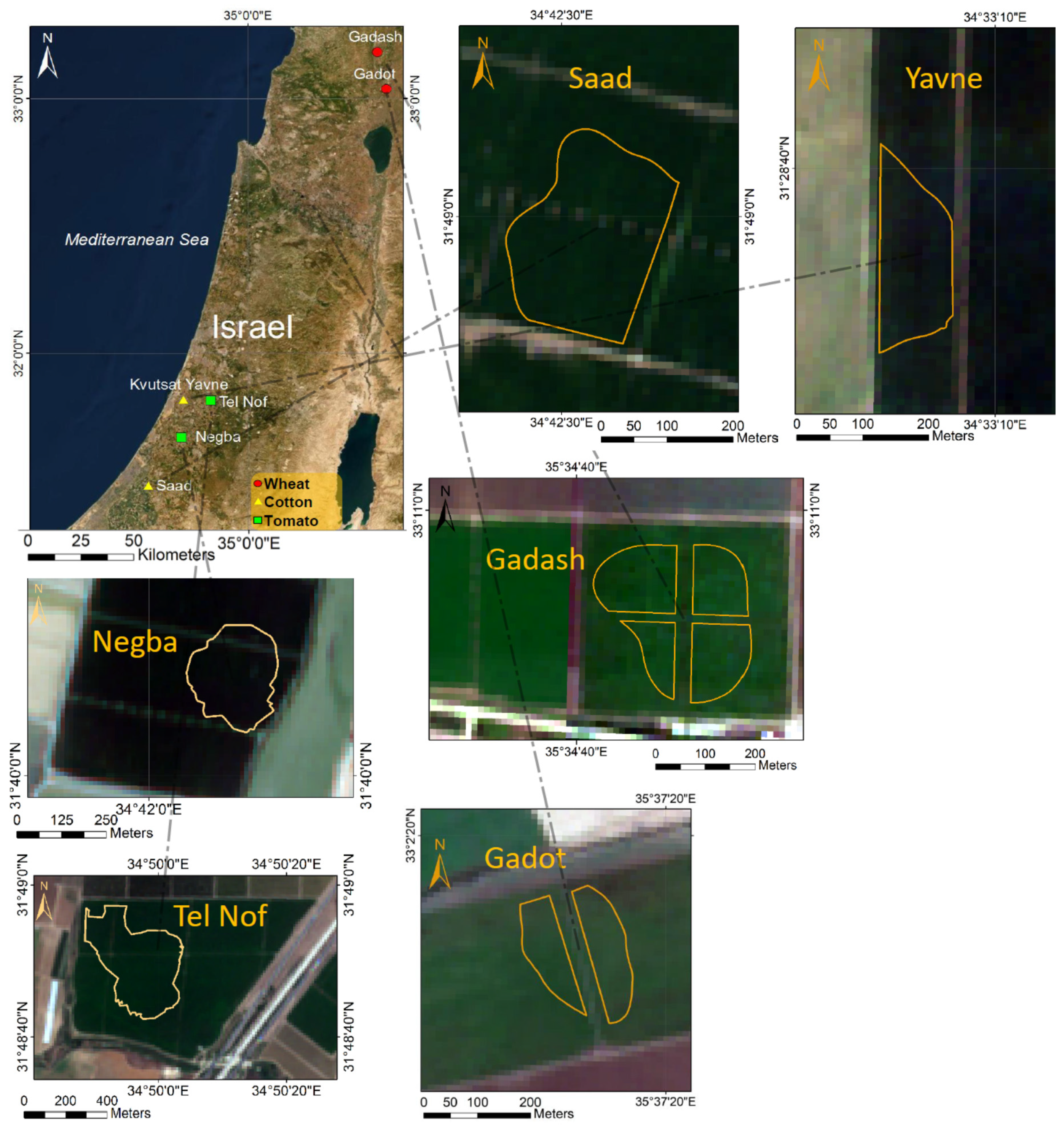
2.1. Test Sites and Field Measurements

The field measurements used in this study were carried out during two seasons of winter wheat, three seasons of processing tomatoes, and two seasons of cotton in different locations in Israel (Table 2, Figure 1). LAI was measured by a SunScan Canopy Analysis System—SS1 developed by Delta-T Company (Cambridge, United Kingdom) during two wheat seasons and two processing tomato seasons. The SunScan is an accurate, nondestructive LAI measurement system successfully employed in many previous studies [25,67]. Each LAI value is an average of at least 30 consecutive field measurements taken at 20-cm intervals along a transect perpendicular to the row direction. Vegetation height was measured at a precision of 1 cm using a tape measure and represented by an average of at least 30 plants per measurement date. LAI and vegetation height in wheat and processing tomatoes were measured throughout the growing seasons; therefore, they represent the full range of these variables. Cotton height was measured during the middle and late stages of one growing season. The backscattering coefficient (σ0) and the radar brightness coefficient (β0) were used in linear scale. Sentinel-1 backscatter values were averaged for a polygon that represented the eddy covariance measurement footprint calculated based on a two-dimensional footprint model [68]. All the empirical regression models in this study utilized the average values of either σ0 or β0, and the local incidence angle (θ) within the areas of interest and same-date field measurements. In cases of gaps in the time series, linearly interpolated values of field measurements from adjacent dates (crop height and LAI) were used. The number of SAR images used for the derivation of the various models was not uniform because each model was based on the period for which field measurements were available, resulting in different numbers of corresponding satellite images. For example, LAI could not be measured using the SunScan system when the plants were very small, while vegetation height was easily measured at any time using a ruler. Accordingly, the LAI models were based on shorter time spans and fewer images than were plant height models. In-field paths and their surrounding area were masked out from analysis polygons of the processing tomato experiments which took place in 2019 to remove bare soil areas and avoid border effects. These excluded areas consisted of approximately 20% of the overall areas of interest. Therefore, the Gadash 2019 area of interest consisted of four vegetated regions separated by paths, and the Gadot 2019 area of interest consisted of two regions.

2.2. Agro-Meteorological Measurements

Agro-meteorological measurements of the reference evapotranspiration (ET0) and actual evapotranspiration (ETc) were performed to derive the crop coefficient (Kc) as Kc = ETc/ET0. Kc is an important variable used to determine the irrigation dose [69]. Daily ETc was derived from water vapor flux measurements by eddy covariance systems [6,70]. The daily ET0 was calculated according to the Penman–Monteith method [33] based on meteorological measurements of air temperature, relative humidity, wind speed, and solar irradiance at the meteorological station closest to the field or at the flux tower itself (Table 2). Meteorological station data are publicly available at http://www.meteo.co.il/ (accessed on 24 June 2021) and http://www.mop-zafon.net/ (accessed on 24 June 2021). The Kc data used for developing the processing tomato models were smoothed in Python with the SciPy library using the cubic and the second-order splines. Smoothing spline is a non-parametric regression technique, which was previously used in various remote sensing applications [15,71,72,73]. ETc was measured throughout the growing seasons of wheat and processing tomatoes and from the middle of the cotton growing seasons. ETc data collected during the Gadash processing tomato experiment in 2018 and the Yavne 2019 wheat experiment were not used for the Kc model development because more than half the data were lost due to technical difficulties that emerged during the experiments.

2.3. Satellite Imagery

Sentinel-1 is part of the European Copernicus program for Earth observation. The payload of the two Sentinel-1 satellites includes a dual-polarization (VV and VH) C-band SAR instrument that is an active phased array antenna working at 5.405 GHz frequency (corresponding wavelength 5.55 cm). The resolution of the Level-1 Ground Range Detected (GRD) Interferometric Wide (IW) mode that was used in this study is 20 × 22 m, with a pixel size of 10 × 10 m, swath width of 250 km, and a revisit time of six days for images with the same geometry. Sentinel-1A and Sentinel-1B were launched on 3 April 2014 and on 25 April 2016, respectively. The Sentinel-1 incidence angle in the IW mode ranges approximately between 29° and 46°. Figure 2 shows the graphical representation of the local incidence angle. In this study, some sites were close to the edge of the images, resulting in an incidence angle range from 30.8° to 45.8°, and in local incidence angle values from 30.3° to 47.7° (Figure 3). Therefore, this study was based on a wide range of incidence angles. The areas within SAR imagery used in the present study are not affected by adverse geometrical effects, such as radar shadow, foreshortening, and layover. The SAR imagery used in this study was downloaded from the ESA Copernicus site (https://scihub.copernicus.eu/dhus/#/home, accessed on 23 June 2021). Overall, 38 SAR images were used to derive models for wheat (Table S1), 19 for cotton (Table S2), and 94 for processing tomatoes (Table S3), Figure 3).

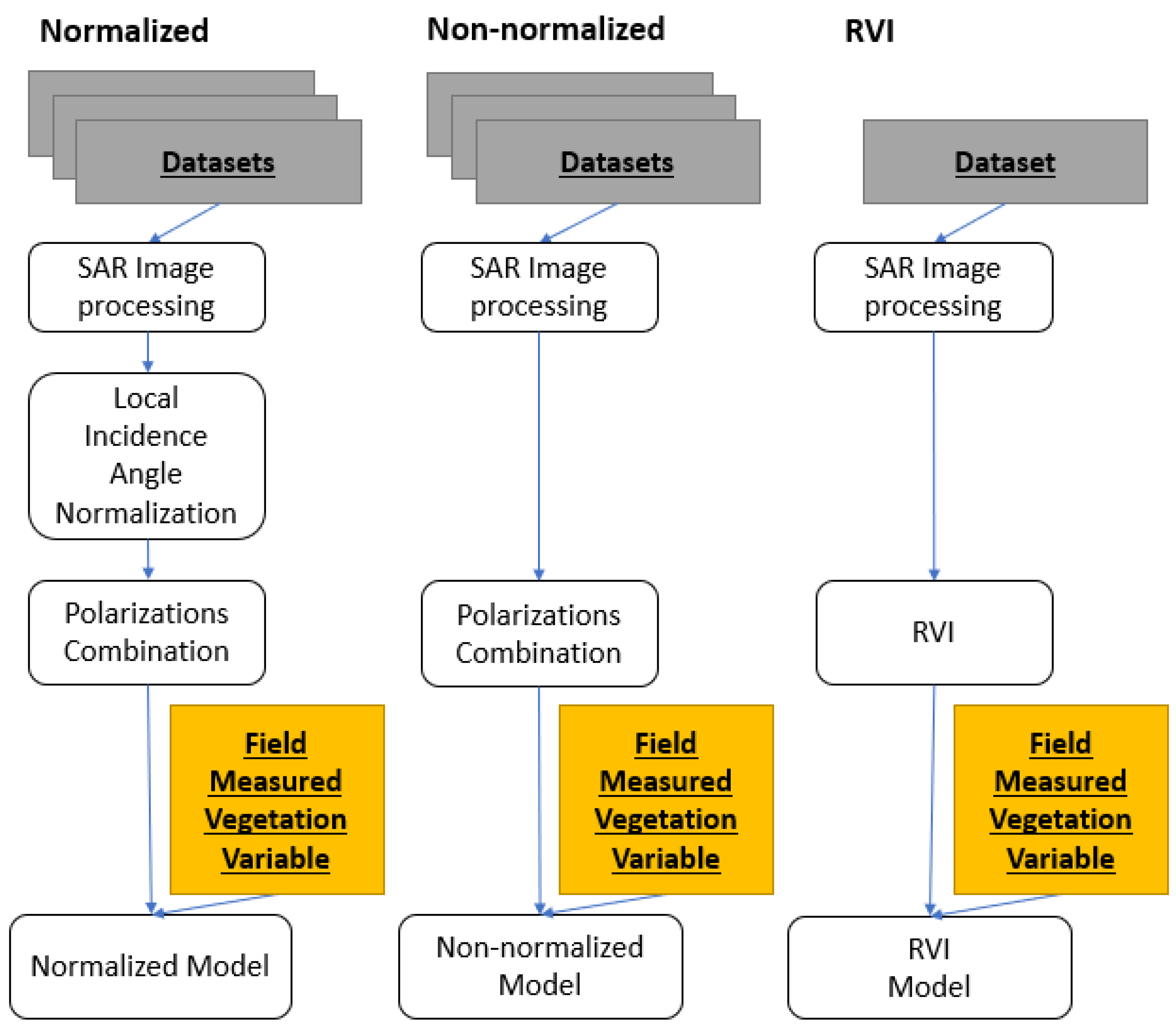
2.4. Image Processing

All images were pre-processed in the Sentinel Application Platform (SNAP versions 6.0 and 7.0, European Space Agency). The sequential pre-processing of the Sentinel-1 imagery was as follows: subsetting a region around the target area, applying the latest orbit file to correct for the satellite path, thermal noise removal, calibration to β0 and σ0 in a natural scale, range Doppler terrain correction using the Shuttle Radar Topography Mission (SRTM, [74]) digital elevation model (DEM) with 30 m resolution. These pre-processing steps were performed in the same sequence as in Song et al. [62], with the addition of the thermal noise removal step that was also performed by Van Tricht et al. [44]. The speckle filtering operation was avoided; therefore, the spatial resolution was retained [75,76,77].

2.5. Dual-Polarized RVI Algorithm

One of the conventional approaches for agricultural monitoring from quad-polarization SAR data is the calculation of the radar vegetation index (RVI) [40]. An adaptation for Sentinel-1 data assumes that σ VV 0 σ HH 0 [78,79,80], such that
RVI = 4 * σ VH 0 σ VH 0 + σ VV 0
The radar backscatter coefficient, σ0, also known as the radar cross-section (RCS) per unit area, is the conventional measure of the intensity of the signal reflected by the surface. It is a normalized dimensionless number that varies significantly with the incidence angle, wavelength, and polarization, as well as with properties of the scattering surface itself [81].
Each RVI model in the present study was based only on one dataset with the maximum number of images acquired at an ascending orbit with the same incidence angle. These are considered to be the most favorable conditions for determining the RVI without incidence angle normalization. An RVI-based Kc model for cotton was not produced because of the lack of imagery acquired at the same incidence angle over the specific fields where the agro-meteorological measurements were performed. The models based on the suggested methods for local incidence angle normalization methods described in Section 2.6 and Section 2.7 were compared to the models based on the RVI.

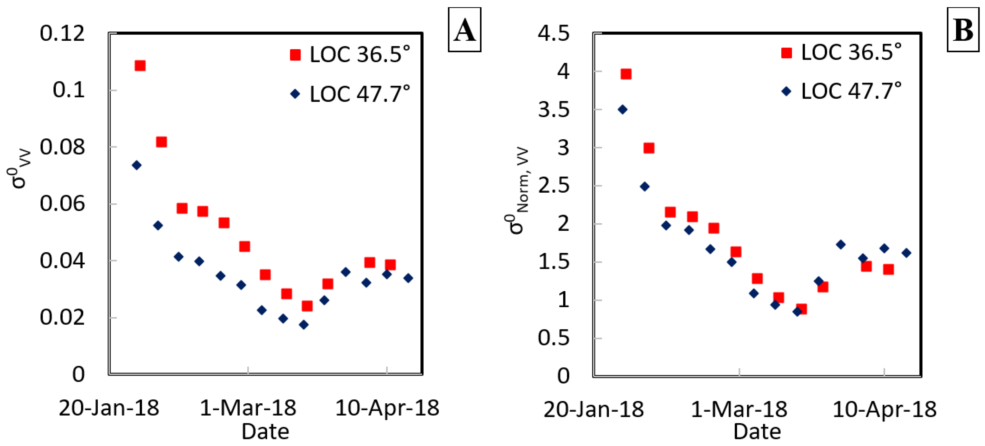
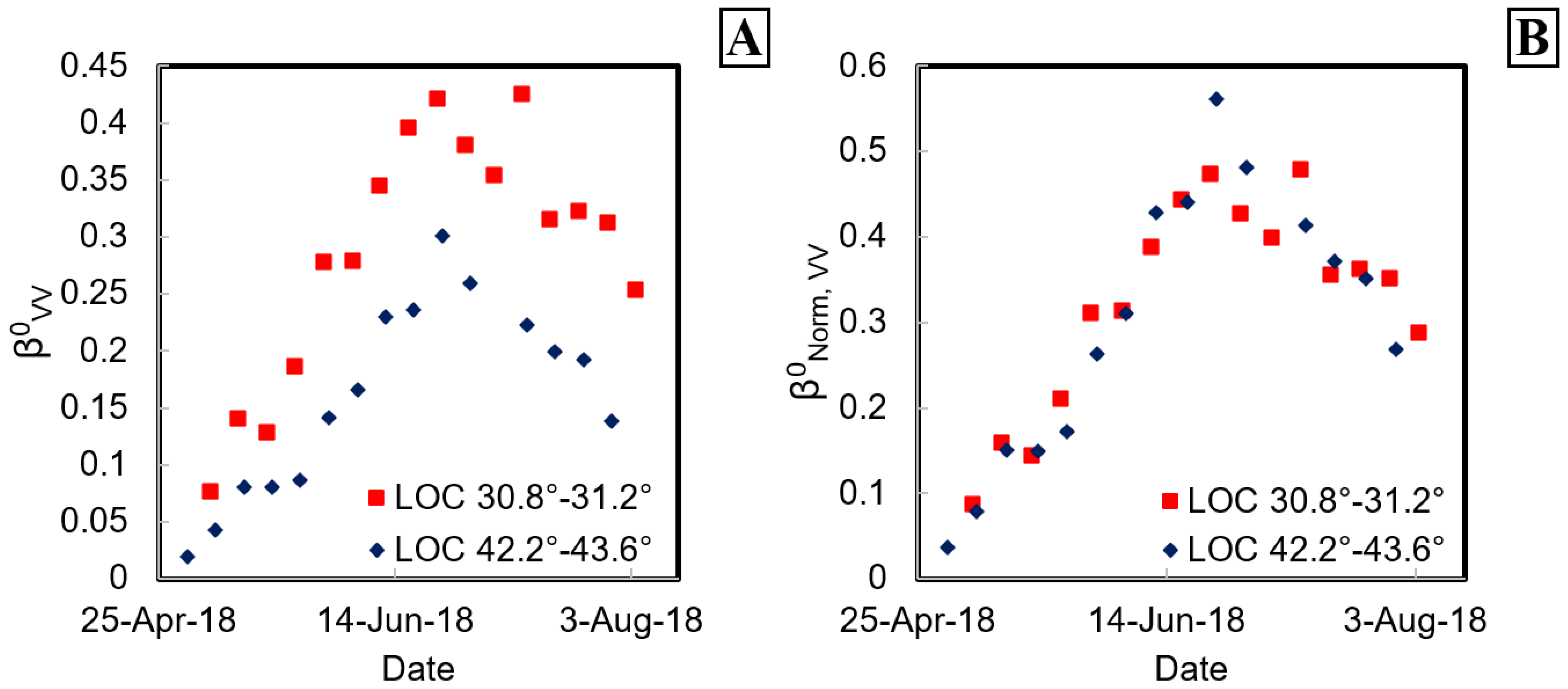
2.6. σ0-Based Local Incidence Angle Normalization

The radar backscatter intensity depends on the incidence angle, with σ0 decreasing proportionally to the incidence angle increase in the intermediate range of incidence angles typical for Sentinel-1 and the majority of spaceborne SAR missions [43,82,83,84]. Based on this understanding, σ0 was normalized by multiplying it with the local incidence angle (θ) in the decimal degree scale:
σ Norm 0 =   σ 0 * θ
The normalization of σ0 is achieved by multiplying lower σ0 values obtained under shallower local incidence angles by higher θ values than the higher σ0 values acquired under steeper local incidence angles. In this study, different VV and VH polarization combinations of normalized σ0 values were used to model Kc, LAI, and crop height. The models described below (Equations (3)–(5)) were produced using polarization combinations that showed the best R2 and RMSE values. The following polarization combination was used to model Kc and LAI in wheat, and LAI in processing tomatoes:
V = σ Norm ,   VH 0 + σ Norm ,   VV 0
where, and afterward, V is a vegetation variable being estimated.
The following polarization combination was used to model wheat and cotton height:
V = σ Norm ,   VH 0 σ Norm ,   VV 0
Processing tomato and cotton Kc estimation models were based on
V = σ Norm ,   VV 0
The descending winter wheat imagery showed a very low correlation with wheat variables and, therefore, was not used for the development of wheat models.

2.7. β0-Based Local Incidence Angle Normalization Method for Tomato and Cotton Height, LAI, and Kc Estimation

A radar beam transmitted at a shallow angle travels longer distances through the vegetation canopy than a beam transmitted under a steep angle; thus, the attenuation of the former is typically higher than that of the latter. Apart from the beam two-way travel distance through the vegetation, the radar backscatter is affected by soil roughness, dielectric properties, and a combination of different types of scatterers that exist in each pixel [85,86]. The wheat fields in this study are flat, and the vegetation growth is uniform. Hence, scattering from the soil surface is mostly specular in the early part of the season, and the volume scattering component increases as the vegetation develops [87,88]. Unlike the wheat fields, the structure of processing tomatoes and cotton fields is more complex, with mounds and furrows. The distance between planted mound centers in all three processing tomato fields is two meters, and it is one meter in cotton. The difference between the elevation of the mounds is up to 15 cm in processing tomatoes and 12 cm in cotton. Consequently, the standard deviation of the surface height is up to 7.5 cm and 6 cm in processing tomatoes and cotton, respectively. According to the Peake and Oliver roughness criterion [89], the surface is considered rough if
h rms > λ 4 * cos   δ
where hrms is the standard deviation of the surface height variation; λ is the wavelength; and δ is the incidence angle. The incidence angle is slightly different from the local incident angle for slopeless surfaces, but this difference does not affect the calculation of the roughness criterion. Accordingly, in C-band SAR with an incidence angle range of 30°–45°, the roughness threshold is hrms > 1.5 cm for an incidence angle of 30°, and hrms > 1.8 cm for an incidence angle of 45°. Therefore, the processing tomato and cotton fields are rough, decreasing backscatter dependence on the incidence angles [85], and modifying the rate of backscatter change as the incidence angle increases [90]. Unlike the smooth wheat fields, every pixel in processing tomato and cotton fields contains multiple types of scattering: specular (plant-free furrows), double bounce (corners between furrows and mounds), and volume scattering in the canopy. Moreover, at some incidence angles, Bragg scattering caused by the row frequency might occur [91,92].
Owing to the complex surface structure in cotton and processing tomato fields, another transformation method specific to these fields was derived empirically in addition to the σ0 normalization method. This new method is based on the polynomial regression between plant variables multiplied by the newly derived attenuation coefficient sin ( Radians ( 90 θ ) 3 ) and radar brightness (β0):
V *   sin ( Radians ( 90 θ ) 3 ) =   A *   ( β 0 ) 2 + B * ( β 0 ) + C
where V is the plant variable (such as height, LAI, or Kc); θ is the local incidence angle in degrees; A, B, and C are the specific model coefficients; and β0 is the radar brightness coefficient [41] at either VV (processing tomatoes) or the sum of VV and VH polarizations (cotton). β0 is a dimensionless coefficient that corresponds to the reflectivity per unit area in the slant range. β0 is used because the radiometric correction of σ0 is based on a sea-level ellipsoid [41,93] and, therefore, less suitable for monitoring of rough surfaces and areas with a rugged topography [94]. Previous studies found β0 to be the best unencumbered estimate SAR measurement [41,95,96]. Using radar brightness is an established practice for research in space [97,98] and common practice in the analysis of RADARSAT-1 imagery [85,99], but not of Sentinel-1 data.
The attenuation coefficient sin ( Radians ( 90 θ ) 3 ) is used to account for the dependence of beam attenuation on the local incidence angle. The SAR beam interaction with objects on the ground can be described as a triangle in which the radar beam is the hypotenuse, and the local incidence angle θ is the angle between the hypotenuse and vertical cathetus normal to the surface (Figure 2). β0 values are reconstructed to a normalized value by applying a sine function to a cubed value of the ( 90 θ ) value in radians. The attenuation coefficient is linearly and inversely proportional to the local incidence angle, as shown in Figure 4. Therefore, by applying the suggested normalization, higher β0 values obtained under steeper (closer to vertical) local incidence angles are divided by higher coefficient values compared to β0 values acquired under shallower local incidence angles. The main difference between the σ0 and β0 methods is that the former applies a steeper increase to the radar backscatter (σ0) as the local incidence angle increases than the latter (β0). This difference in the behavior of the methods was created to take into account that as the incidence angle increases, the radar backscatter decreases more slowly for rough surfaces than for smooth surfaces [90,100].
Therefore, the normalized β0 value can be written as
β Norm 0 = β 0 sin ( Radians ( 90 θ ) 3 )
where β N o r m 0 is the normalized radar brightness in VV or VH polarization, β0 is the radar brightness in VV or VH polarization, and sin ( Radians ( 90 θ ) 3 ) is the attenuation coefficient.
The processing tomato LAI model utilizes the sum of normalized β0 in both polarizations:
LAI = β VH 0 sin ( Radians ( 90 θ ) 3 ) + β VV 0 sin ( Radians ( 90 θ ) 3 )

2.8. Calibration and Validation of Empirical Vegetation Variable Estimation Models

The field-measured vegetation variables were used in regression models against the uncorrected radar backscatter parameters. Further, the proposed local incidence angle normalization methods were applied to the SAR images, and new empirical regression models were derived. Finally, the models based on the data prior to normalization and post-normalization and on the dual-polarized RVI were compared to assess the performance of the normalization process (Figure 5).
In every case, the same type of regression model (either linear or polynomial) and the same polarization combination were used in the comparison. Coefficients of determination in models based on non-normalized data were symbolized as R 0 2 , and their root-mean-square error was symbolized as RMSE0. The differences in the R2 and RMSE following the normalization procedures were calculated. In addition, the Steiger variation [101] of the two-tailed Fisher Z-score tests [102] was performed to determine whether the difference in the models’ R2 is significant (α ≤ 0.05). The significance of the RMSE difference was calculated using the two-tailed Wilcoxon signed-rank test [103] to determine whether the difference in the models’ RMSE was significant (α ≤ 0.05). According to the goals set in this study and due to a finite amount of available SAR imagery and ground truth data, all the available data were used to calibrate the empirical models to achieve the models’ maximum reliability and estimation accuracy [104]. In order to additionally validate the models’ estimation performance, the RMSE values of normalized models applied separately to each dataset (experiment) were also calculated and are presented in Tables S4–S8.

3. Results

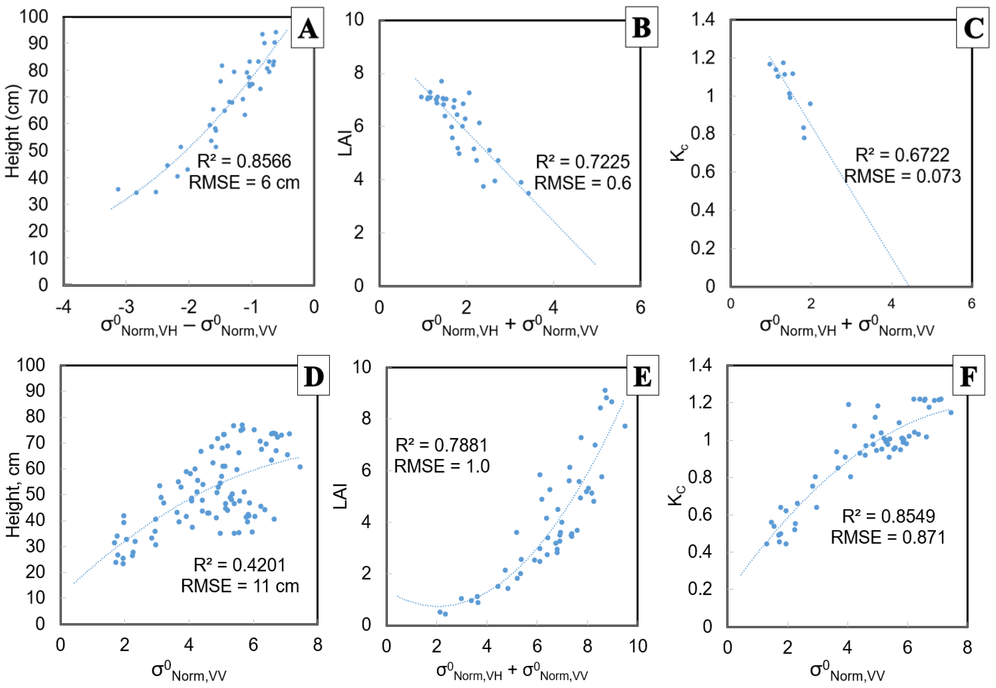
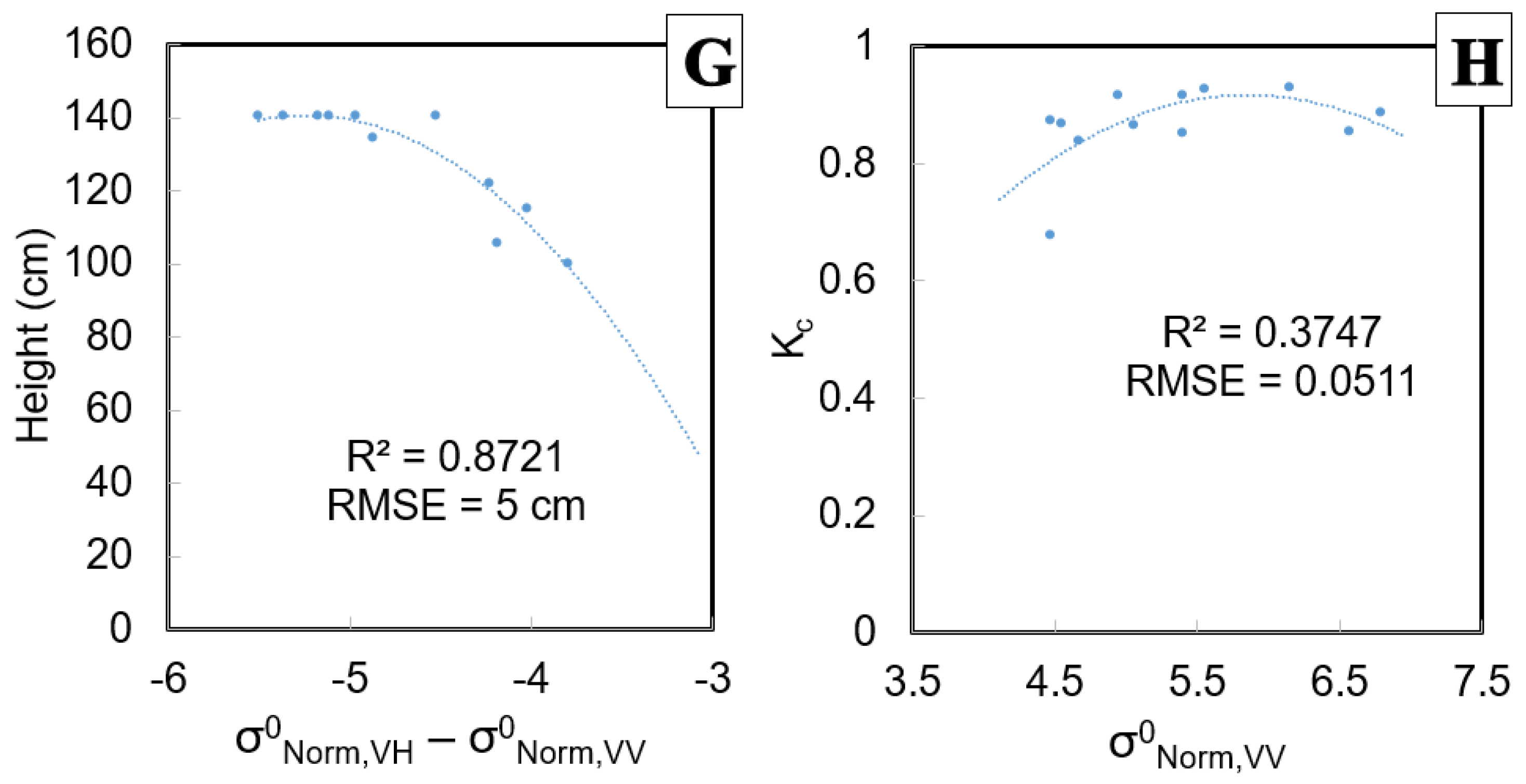
3.1. Wheat, Processing Tomato, and Cotton Height, LAI, and Kc Models Based on the σ0 Normalization Method

The effect of the proposed normalization (Equation (2)) on the SAR backscatter from two incidence angles is illustrated in Figure 6. Following the normalization process, the difference is greatly reduced, and a considerable improvement in the R2 and RMSE of all the σ0-based models is observed. In wheat, processing tomatoes, and cotton, the height, LAI, and Kc models’ R2 improved in the range of 0.0172–0.367, and the RMSE improved in the range of 5–52%. Table 3, Tables S4–S6, and Figure 7 show the performance of σ0-based height, LAI, and Kc models in wheat, processing tomatoes, and cotton.

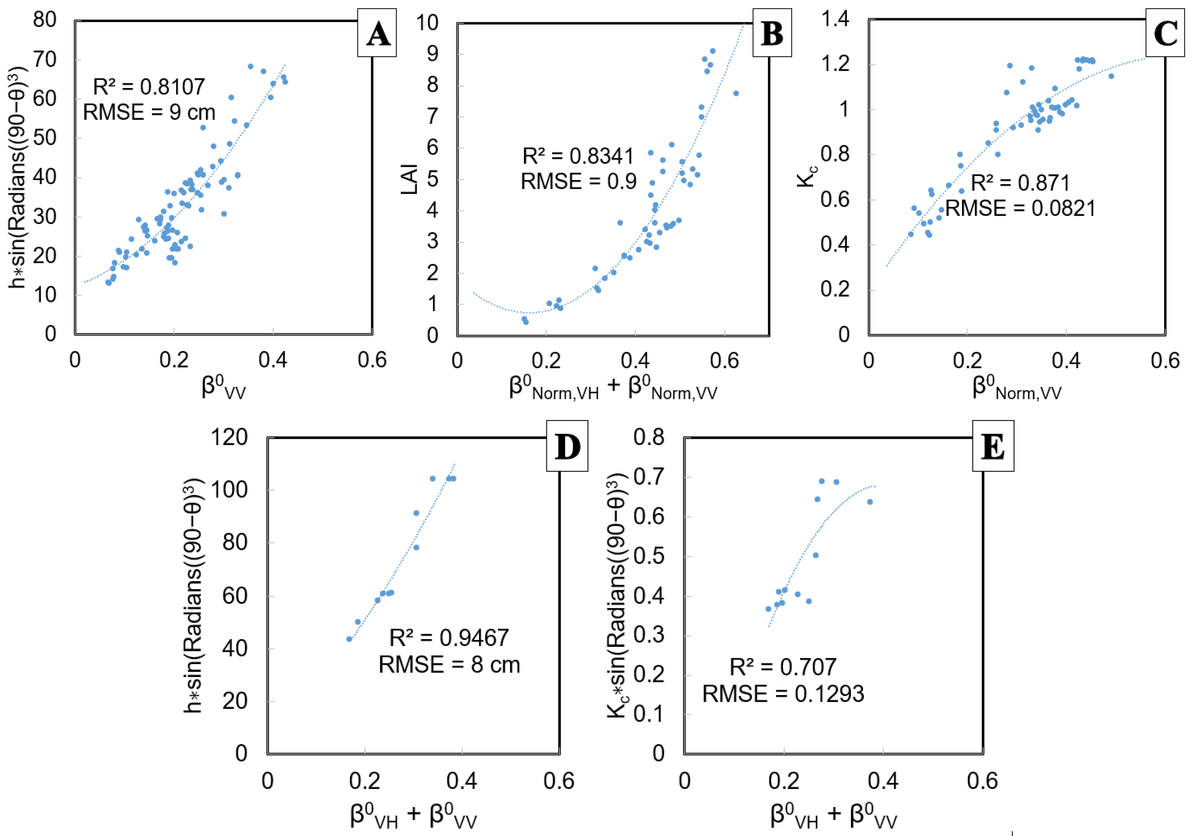
3.2. Processing Tomato and Cotton Height, LAI, and Kc Models Based on the β0 Normalization Method

The effect of the β0-based normalization (Equation (8)) that reduces the difference in β0 images acquired at different angles is shown in Figure 8.
The β0-based normalization method permitted achieving the improvement in the R2 and RMSE of all the β0-based models. For the processing tomato and cotton height, LAI, and Kc models, the R2 improved in the range of 0.1143–0.668, and the RMSE improved in the range of 18–44%. Table 3, Tables S7 and S8, and Figure 9 show the performance of processing tomato and cotton β0-based height, LAI, and Kc models. Table 3 shows the performance of all the σ0-based and β0-based normalized models developed in this study and their R2 and RMSE improvements over the non-normalized models.

3.3. Performance of the Dual-Polarized RVI

The dual-polarized RVI-based wheat, processing tomato, and cotton models are shown in Table 4. The wheat and cotton RVI models were compared against the σ0-based models, while the processing tomato RVI models were compared to the β0-based processing tomato models.

4. Discussion

In contrast with previous studies that mostly used images acquired under fixed or within narrow ranges of incidence angles, the correction derived in this study facilitates the use of imagery acquired under all typical geometrical conditions. By applying simple transformations to Sentinel-1 imagery acquired under a wide range of incidence angles, the dependency of σ0 and β0 on the local incidence angle decreased, and the empirical modeling of several crop properties was improved. This achievement is remarkable because monitoring crops using the full temporal resolution of SAR imagery is much more useful than using imagery acquired at a narrow range of angles. Moreover, vegetation variable estimation models calibrated in one region using the proposed methods can be applied to other areas.
The improvement in the R2 and RMSE of the models following the local incidence angle normalization procedure was found to be significant in many of the models: wheat height and LAI models; β0-based processing tomato LAI, height, and Kc models; σ0-based cotton Kc and height models; and β0-based cotton height model. Since the statistical significance of the difference between correlations is dependent on the number of images used for model development, some of the models yielded a difference that was not significant (wheat Kc model, processing tomato σ0-based LAI, height, and Kc models, and cotton Kc β0-based model). However, the trend of improvement following the proposed normalization procedures is clear, and the practical usefulness of the proposed methods can be better represented by the RMSE improvements because RMSE represents the vegetation variable estimation accuracy. The RMSE improvement was found to be significant in the following models: processing tomato σ0-based LAI and Kc models; and cotton Kc σ0 and β0-based models. The RMSE improvement was not significant in the following models: wheat, processing tomato σ0-based LAI, and processing tomato β0-based models, and cotton height σ0- and β0-based models. The R2 and RMSE of all the models calibrated in the present study improved following incidence angle normalization. The range of RMSE improvements varied from model to model (Table 3), from 5 to 52%. Moreover, the performance of the newly developed β0-based local incidence angle normalization method shows potential for overcoming the limitations of σ0-based modeling for agricultural purposes. The use of β0 to improve vegetation variable estimation is particularly useful in fields with a rough soil surface geometry. Using β0 is not common for Sentinel-1 imagery, and the users’ community could benefit from adopting this approach.
The models presented here for wheat and processing tomatoes were calibrated based on measurements taken throughout the entire duration of growing seasons and can, therefore, be applied at any time during crop development without restrictions. Nevertheless, the RMSE of LAI and height estimations was slightly higher at the peak of the season compared to the rest of the season. The relatively high accuracy of the models calibrated in this study and their independence from the incidence angle following the new normalization methods are advantageous compared to previous studies [47,55,60,61,64], in which the images used were limited to a narrow range of incidence angles. In addition, in contrast to [48] that presented models that can only be reliably applied to certain vegetation heights, the wheat and processing tomato models presented here are applicable to any height within the range measured in our experiments: 34–95 cm (wheat) and 24–77 cm (processing tomatoes). A comparison between several studies that used C-band SAR to estimate vegetation height and LAI is shown in Table 5 and Table 6.
The models for LAI estimation show a better performance than previous studies. Previous estimation based on imagery acquired under a narrow range of incidence angles and dual-polarization [47] only achieved R2 = 0.25. Moreover, the models in this study performed similarly to quad-polarization RADARSAT-2-based models for corn and soybean LAI estimation that utilized imagery acquired under a narrow range of incidence angles [39] and achieved R2 = 0.66 and RMSE = 0.75 and R2 = 0.64 and RMSE = 0.63, respectively. Another study [60] presented a wheat LAI estimation model, which has better prediction performance than the models obtained in the present study (RMSE = 0.4), but as in other previous models, it was based on images acquired under only one incidence angle. Unlike the LAI estimation based on optical imagery, the wheat and processing tomato LAI models developed in this study were not saturated even at the peak of vegetation development (wheat LAImax = 7.7, processing tomato LAImax = 9.1). Therefore, the LAI models in this paper might be applied throughout the whole season duration, which is useful because the LAI is a proxy for many vegetation variables [23], including crop productivity [105].
The use of SAR for agricultural purposes has also been significantly enhanced by this study. While several previous studies used SAR to estimate the wheat LAI and crop height, processing tomatoes were not studied enough. Moreover, estimating Kc of wheat, processing tomatoes, and cotton by SAR, to the best of our knowledge, was not previously conducted. Previously, the crop water requirement estimation of maize, soybean, pasture, and bean using SAR imagery acquired under a narrow range of incidence angles was conducted [49]. Another study showed a non-crop-specific region-wise correlation between only one Sentinel-1 image and the crop water stress index derived through the LANDSAT-8 image [106]. Finally, [107] used smoothed time series of Sentinel-1 backscatter values in different polarization combinations to estimate Kc in vineyards. Therefore, the wheat and processing tomato Kc estimation models derived in this study pave the way to accurate Kc estimation using all available SAR imagery. This study stands out by overcoming the limits imposed by the range of incidence angles typical for SAR imagery. As a result, the newly developed normalized wheat and processing tomato Kc estimation models can be used with confidence during the entire duration of a growing season.
Although the cotton models calibrated in this study showed good performance, they are based on the data recorded from the middle to late stages of growing seasons. Therefore, future studies should improve upon this by including the early stages of the growing seasons. In addition, we did not calibrate an LAI model for cotton in this paper, but this should be feasible given good field measurements. Therefore, additional field experiments should be carried out to calibrate models for crop variables throughout the growing season. Even though the cotton models developed in this study might have only limited use, all four cotton models showed a sizeable improvement in the R2 and RMSE over the non-normalized models. This result confirms the effectiveness of the novel angle normalization approach suggested in the present study.
The performance of models based on the new transformation was favorable compared to models based on the dual-polarized RVI. Although the RVI-based models in the present study were calibrated under the most favorable conditions possible, using only ascending overpass imagery acquired under only one incidence angle, the new models based on local incidence angle normalization methods outperformed them: the RMSE of RVI-based models was 40–203% higher. It should be noted that the assumption σ VV 0 σ HH 0 underlying the dual-polarized RVI is in contradiction to previous findings that show a typical difference of 5 dB between σ VV 0 and σ HH 0 in the intermediate range of incidence angles in the C band [91,108,109]. Therefore, we conclude that the dual-polarized RVI is not recommended where the assumption of the equality of backscatter in the two polarizations cannot be made.
Unlike previous studies that used only fields with rows perpendicular to the SAR beam [110], in this study, all the fields were used in model calibration. While this row geometry is less noticeable in wheat fields, particularly in the middle and later stages of the season, it should be noted that cotton and processing tomatoes are planted in rows of earth mounds with furrows between them. In addition, the spatial orientation of the rows in the fields in this study was not uniform between the locations. For example, in the processing tomato fields in Gadash, the rows were oriented from west to east, while in Gadot, the orientation was from west-southwest to east-northeast. This difference in the spatial orientation of rows affects the backscatter because the target’s radar cross-section depends on its angle relative to the satellite [111], and even minimal changes in the target aspect significantly affect the RCS [112,113]. Nevertheless, the processing tomato models were not sensitive to the crop row orientation because they showed a similar RMSE (Tables S5 and S7) when they were applied to different fields. Therefore, the proposed models seem to be insensitive to the row orientation and could likely be used in other fields with different row orientations relative to the satellite orbit. However, this should be further tested in future studies.
Despite the overall reliable performance of the newly developed models, it should be pointed out that winter images in descending orbits have much weaker correlations with the vegetation height, LAI, and Kc compared to images from ascending orbits. Consequently, SAR images acquired in descending orbits could not be used for the development of the wheat model. In the summer crops tested in this study, this phenomenon did not occur, rendering the imagery acquired from descending orbits usable for the modeling of crop variables.
A likely explanation for the weaker performance of wheat models based on imagery from descending orbits might be related to the higher relative humidity in the early morning (descending images were acquired around 03:40 GMT) compared to the relative humidity in the evening (ascending images were acquired around 15:40 GMT). This observation is confirmed by our meteorological measurements in Saad and Kvutsat Yavne, which showed a regular diurnal pattern of a decrease in relative humidity following sunrise: from up to 100% in early morning hours to 40–60% in the afternoons. At night and in the early morning, the relative humidity is very high, and the formation of fog and dew, along with increased topsoil moisture, causes increased scattering and attenuation of the SAR beam [114,115]. Additionally, the SAR beam can be affected by common atmospheric inhomogeneities in the morning hours over Israel that create radar echoes [116] and increase the atmospheric reflectance and attenuation of the transmitted energy [117]. In previous studies, datasets affected by these effects were binned. For example, [61] omitted a dataset that was affected by dew. The issue of the relatively lower performance of descending orbit-based models is an interesting direction that can be studied by analyzing data from other regions and coupling them with the complementary ground and atmospheric measurements.
Although the newly proposed local incidence angle normalization methods were tested on the typical incidence angle range of Sentinel-1 and most other spaceborne SAR missions, they are not expected to be effective for very steep incidence angles near to the “nadir hole” region [118] or for very shallow angles because of the non-linear dependence of the radar backscatter on the incidence angle in these ranges [90,91].
The proposed σ0 local incidence angle normalization method can be used not only for agricultural purposes but also for other SAR applications. Additional studies need to be carried out to determine if this method is ideal for general use. The β0 local incidence angle normalization method might be used for the vegetation variable estimation of crops other than processing tomatoes and cotton grown on rough soil surfaces. Future studies should pursue this.

5. Conclusions

The proposed σ0 and β0 local incidence angle normalization methods facilitate the use of all the images acquired by the Sentinel-1 constellation under the full range of typical incidence angles. This is supported by an improvement in the correlations between the SAR measurements and crop variables such as LAI, crop height, and Kc following these normalization procedures in three crops: cotton, tomatoes, and wheat. Models based on the suggested normalization of the incidence angle show considerable R2 and RMSE improvements over the models that were not based on these transformations. This increase in performance is the most notable for the wheat height and LAI models, processing tomato σ0-based LAI and β0-based height models, and the cotton models. Most Kc, LAI, and height models worked well with imagery acquired from ascending and descending orbits, but winter imagery performed better with ascending orbits. This approach to estimate vegetation variables is useful for routine vegetation and agricultural monitoring, having a higher temporal resolution and accuracy than the previous approaches. Despite these results, we wish to stress that the most important achievement is not only the improvement in the models’ performance but also the enablement of the conjoint use of images acquired under different incidence angles and even different orbits.

Supplementary Materials

The following are available online at https://0-www-mdpi-com.brum.beds.ac.uk/article/10.3390/land10070680/s1; Table S1: Sentinel-1 image inventory used in the development of models for wheat. Each line represents a dataset with specific geometrical parameters; Table S2: Sentinel-1 image inventory used in the development of models for cotton. Each line represents a dataset with specific geometrical parameters; Table S3: Sentinel-1 image inventory used in the development of models for processing tomatoes. Each line represents a dataset with specific geometrical parameters; Table S4: Wheat height, LAI, and Kc models; Table S5: Processing tomato height, LAI, and Kc models based on the σ0 normalization method; Table S6: Cotton height and Kc models based on the σ0 normalization method; Table S7: Processing tomato height, LAI, and Kc models based on the β0 normalization methods; Table S8: Cotton height and Kc models based on the β0 normalization method.

Author Contributions

Conceptualization, O.R., G.K.; methodology, G.K., software, G.K., L.F., V.L.; validation, G.K.; formal analysis, G.K.; investigation, G.K.; fieldwork, G.K., V.L., L.F., V.S.M.; writing—original draft preparation, G.K., O.R.; writing—review and editing, O.R., G.K., V.S.M., J.T.; visualization, G.K., V.S.M., O.R.; supervision, O.R.; project administration, O.R., J.T.; funding acquisition, O.R., J.T. All authors have read and agreed to the published version of the manuscript.

Funding

The cotton field measurements were funded by the Chief Scientist of the Ministry of Agriculture, Israel, under grant number 304-0505, and the wheat and tomato field measurements were funded by the Ministry of Science and Technology, Israel, under grant numbers 3-14559, 3-15605. Gregoriy Kaplan was supported by an absorption grant for new immigrant scientists provided by the Israeli Ministry of Immigrant Absorption. Manivasagam V.S. was supported by the ARO Postdoctoral Fellowship Program from the Agriculture Research Organization, Volcani Institute, Israel.

Institutional Review Board Statement

Not applicable.

Informed Consent Statement

Not applicable.

Data Availability Statement

Sentinel-1 data were obtained from the ESA Copernicus Open Access Hub website (https://scihub.copernicus.eu/dhus/#/home, accessed on 26 June 2021).

Acknowledgments

We thank Leonid Dinevich from Tel-Aviv University for his helpful advice. We thank Nitai Haymann for his contribution to software processing and fieldwork. We thank all the growers. We also thank the reviewers.

Conflicts of Interest

The authors declare no conflict of interest.

References

  1. Broge, N.H.; Thomsen, A.G.; Andersen, P.B. Comparison of Selected Vegetation Indices as Indicators of Crop Status. Available online: http://www.earsel.org/symposia/2002-symposium-Prague/pdf/083.pdf (accessed on 24 June 2021).
  2. González-Dugo, M.P.; Mateos, L. Spectral vegetation indices for benchmarking water productivity of irrigated cotton and sugarbeet crops. Agric. Water Manag. 2008, 95, 48–58. [Google Scholar] [CrossRef]
  3. Johnson, L.F.; Trout, T.J. Satellite NDVI Assisted Monitoring of Vegetable Crop Evapotranspiration in California’s San Joaquin Valley. Remote Sens. 2012, 4, 439–455. [Google Scholar] [CrossRef] [Green Version]
  4. Mróz, M.; Sobieraj, A. Comparison of several vegetation indices calculated on the basis of a seasonal SPOT XS time series, and their suitability for land cover and agricultural crop identification. Technol. Sci. 2004, 7, 39–66. [Google Scholar] [CrossRef]
  5. Purevdorj, T.S.; Tateishi, R.; Ishiyama, T.; Honda, Y. Relationships between percent vegetation cover and vegetation indices. Int. J. Remote Sens. 1998, 19, 3519–3535. [Google Scholar] [CrossRef]
  6. Rozenstein, O.; Haymann, N.; Kaplan, G.; Tanny, J. Estimating cotton water consumption using a time series of Sentinel-2 imagery. Agric. Water Manag. 2018, 207, 44–52. [Google Scholar] [CrossRef]
  7. Santos, C.L.M.d.O.; Lamparelli, R.A.C.; Figueiredo, G.K.D.A.; Dupuy, S.; Boury, J.; Luciano, A.C.d.S.; Torres, R.d.S.; le Maire, G. Classification of crops, pastures, and tree plantations along the season with multi-sensor image time series in a subtropical agricultural region. Remote Sens. 2019, 11, 334. [Google Scholar] [CrossRef] [Green Version]
  8. Viña, A.; Gitelson, A.A.; Nguy-Robertson, A.L.; Peng, Y. Comparison of different vegetation indices for the remote assessment of green leaf area index of crops. Remote Sens. Environ. 2011, 115, 3468–3478. [Google Scholar] [CrossRef]
  9. Nguy-Robertson, A.L.; Peng, Y.; Gitelson, A.A.; Arkebauer, T.J. Agricultural and Forest Meteorology Estimating green LAI in four crops Potential of determining optimal spectral bands for a universal algorithm. Agric. For. Meteorol. J. 2014, 192–193, 140–148. [Google Scholar] [CrossRef]
  10. Rozenstein, O.; Qin, Z.; Derimian, Y.; Karnieli, A. Derivation of land surface temperature for Landsat-8 TIRS using a split window algorithm. Sensors 2014, 14, 5768–5780. [Google Scholar] [CrossRef]
  11. Manivasagam, V.S.; Kaplan, G.; Rozenstein, O. Developing Transformation Functions for VENμS and Sentinel-2 Surface Reflectance over Israel. Remote Sens. 2019, 11, 1710. [Google Scholar] [CrossRef] [Green Version]
  12. Flood, N. Continuity of reflectance data between Landsat-7 ETM+ and Landsat-8 OLI, for both top-of-atmosphere and surface reflectance: A study in the Australian landscape. Remote Sens. 2014, 6, 7952–7970. [Google Scholar] [CrossRef] [Green Version]
  13. Bannari, A. Synergy Between Sentinel-MSI and Landsat-OLI to Support High Temporal Frequency for Soil Salinity Monitoring in an Arid Landscape. Res. Dev. Saline Agric. 2019. [Google Scholar] [CrossRef]
  14. Padró, J.C.; Pons, X.; Aragonés, D.; Díaz-Delgado, R.; García, D.; Bustamante, J.; Pesquer, L.; Domingo-Marimon, C.; González-Guerrero, Ò.; Cristóbal, J.; et al. Radiometric correction of simultaneously acquired Landsat-7/Landsat-8 and Sentinel-2A imagery using Pseudoinvariant Areas (PIA): Contributing to the Landsat time series legacy. Remote Sens. 2017, 9, 1319. [Google Scholar] [CrossRef] [Green Version]
  15. Kaplan, G.; Fine, L.; Lukyanov, V.; Manivasagam, V.S.; Malachy, N.; Tanny, J.; Rozenstein, O. Estimating Processing Tomato Water Consumption, Leaf Area Index, and Height Using Sentinel-2 and VENµS Imagery. Remote Sens. 2021, 13, 1046. [Google Scholar] [CrossRef]
  16. Asrar, G.; Fuchs, M.; Kanemasu, E.T.; Hatfield, J.L. Estimating Absorbed Photosynthetic Radiation and Leaf Area Index from Spectral Reflectance in Wheat. Agron. J. 1984, 76, 300. [Google Scholar] [CrossRef]
  17. Reichenau, T.G.; Korres, W.; Montzka, C.; Fiener, P.; Wilken, F.; Stadler, A.; Waldhoff, G.; Schneider, K. Spatial heterogeneity of Leaf Area Index (LAI) and its temporal course on arable land: Combining field measurements, remote sensing and simulation in a Comprehensive Data Analysis Approach (CDAA). PLoS ONE 2016, 11, 1–24. [Google Scholar] [CrossRef] [PubMed] [Green Version]
  18. Sun, Y.; Qin, Q.; Ren, H.; Zhang, T.; Chen, S. Red-Edge Band Vegetation Indices for Leaf Area Index Estimation from Sentinel-2/MSI Imagery. IEEE Trans. Geosci. Remote Sens. 2020, 58, 826–840. [Google Scholar] [CrossRef]
  19. Wang, C.; Feng, M.C.; Yang, W.D.; Ding, G.W.; Sun, H.; Liang, Z.Y.; Xie, Y.K.; Qiao, X.X. Impact of spectral saturation on leaf area index and aboveground biomass estimation of winter wheat. Spectrosc. Lett. 2016, 49, 241–248. [Google Scholar] [CrossRef]
  20. Kaplan, G.; Rozenstein, O. Spaceborne Estimation of Leaf Area Index in Cotton, Tomato, and Wheat Using Sentinel-2. Land 2021, 10, 505. [Google Scholar] [CrossRef]
  21. Simic Milas, A.; Romanko, M.; Reil, P.; Abeysinghe, T.; Marambe, A. The importance of leaf area index in mapping chlorophyll content of corn under different agricultural treatments using UAV images. Int. J. Remote Sens. 2018, 39, 5415–5431. [Google Scholar] [CrossRef]
  22. Ewert, F. Modelling plant responses to elevated CO2: How important is leaf area index? Ann. Bot. 2004, 93, 619–627. [Google Scholar] [CrossRef] [Green Version]
  23. Herrmann, I.; Pimstein, A.; Karnieli, A.; Cohen, Y.; Alchanatis, V.; Bonfil, D.J. LAI assessment of wheat and potato crops by VENμS and Sentinel-2 bands. Remote Sens. Environ. 2011, 115, 2141–2151. [Google Scholar] [CrossRef]
  24. Heuvelink, E.; Bakker, M.J.; Elings, A.; Kaarsemaker, R.; Marcelis, L.F.M. Effect of leaf area on tomato yield. Acta Hortic. 2005, 691, 43–50. [Google Scholar] [CrossRef]
  25. Sadeh, Y.; Zhu, X.; Dunkerley, D.; Walker, J.P.; Zhang, Y.; Rozenstein, O.; Manivasagam, V.S.; Chenu, K. Fusion of Sentinel-2 and PlanetScope time-series data into daily 3 m surface reflectance and wheat LAI monitoring. Int. J. Appl. Earth Obs. Geoinf. 2021, 96, 102260. [Google Scholar] [CrossRef]
  26. Manivasagam, V.S.; Rozenstein, O. Practices for upscaling crop simulation models from field scale to large regions. Comput. Electron. Agric. 2020, 175, 105554. [Google Scholar] [CrossRef]
  27. Manivasagam, V.S.; Sadeh, Y.; Kaplan, G.; Bonfil, D.J.; Rozenstein, O. Studying the Feasibility of Assimilating Sentinel-2 and PlanetScope Imagery into the SAFY Crop Model to Predict Within-Field Wheat Yield. Remote Sens. 2021, 13, 2395. [Google Scholar] [CrossRef]
  28. Qi, J.; Wang, C.; Inoue, Y.; Zhang, R.; Gao, W. Synergy of optical and radar remote sensing in agricultural applications. Ecosyst. Dyn. Agric. Remote Sens. Model. Site-Specific Agric. 2004, 5153, 153. [Google Scholar] [CrossRef]
  29. Luo, P.; Liao, J.; Shen, G. Combining Spectral and Texture Features for Estimating Leaf Area Index and Biomass of Maize Using Sentinel-1/2, and Landsat-8 Data. IEEE Access 2020, 8, 53614–53626. [Google Scholar] [CrossRef]
  30. Jin, X.; Yang, G.; Xu, X.; Yang, H.; Feng, H.; Li, Z.; Shen, J.; Zhao, C.; Lan, Y. Combined multi-temporal optical and radar parameters for estimating LAI and biomass in winter wheat using HJ and RADARSAR-2 data. Remote Sens. 2015, 7, 13251–13272. [Google Scholar] [CrossRef] [Green Version]
  31. Wang, J.; Xiao, X.; Bajgain, R.; Starks, P.; Steiner, J.; Doughty, R.B.; Chang, Q. Estimating leaf area index and aboveground biomass of grazing pastures using Sentinel-1, Sentinel-2 and Landsat images. ISPRS J. Photogramm. Remote Sens. 2019, 154, 189–201. [Google Scholar] [CrossRef] [Green Version]
  32. Reamer, R.E.; Stockton, W.O.; Stromfors, R.D. New military uses for Synthetic Aperture Radar (SAR). Airborne Reconnaiss. XVI 1993, 113–119. [Google Scholar] [CrossRef]
  33. Allen, R.G.; Pereira, L.S.; Dirk, R.; Smith, M. Crop Evapotranspiration-Guidelines For Computing Crop Water Requirements-FAO Irrigation And Drainage Paper 56; FAO: Rome, Italy, 1998; Volume 300, p. D05109. Available online: http://www.fao.org/3/X0490E/X0490E00.htm (accessed on 24 June 2021).
  34. Pereira, L.S.; Paredes, P.; Hunsaker, D.J.; López-Urrea, R.; Mohammadi Shad, Z. Standard single and basal crop coefficients for field crops. Updates and advances to the FAO56 crop water requirements method. Agric. Water Manag. 2021, 243, 1–35. [Google Scholar] [CrossRef]
  35. Trevisan, R.G.; Junior, N.d.S.V.; Portz, G.; Eitelwein, M.T.; Molin, J.P. Use of crop height and optical sensor readings to predict mid-season cotton biomass. In Proceedings of the Precision agriculture ’15, Volcani Center, Israel, 12–16 July 2015; p. 8. [Google Scholar]
  36. Asilo, S.; Nelson, A.; Bie, K.D.; Skidmore, A.; Laborte, A.; Maunahan, A.; Quilang, E.J.P. Relating X-band SAR Backscattering to Leaf Area Index of Rice in Different Phenological Phases. Remote Sens. 2019, 11, 1462. [Google Scholar] [CrossRef] [Green Version]
  37. Canisius, F.; Shang, J.; Liu, J.; Huang, X.; Ma, B.; Jiao, X.; Geng, X.; Kovacs, J.M.; Walters, D. Tracking crop phenological development using multi-temporal polarimetric Radarsat-2 data. Remote Sens. Environ. 2018, 210, 508–518. [Google Scholar] [CrossRef]
  38. McNairn, H.; Champagne, C.; Shang, J.; Holmstrom, D.; Reichert, G. Integration of optical and Synthetic Aperture Radar (SAR) imagery for delivering operational annual crop inventories. ISPRS J. Photogramm. Remote Sens. 2009, 64, 434–449. [Google Scholar] [CrossRef]
  39. Hosseini, M.; McNairn, H.; Merzouki, A.; Pacheco, A. Estimation of Leaf Area Index (LAI) in corn and soybeans using multi-polarization C- and L-band radar data. Remote Sens. Environ. 2015, 170, 77–89. [Google Scholar] [CrossRef]
  40. Kim, Y.; Jackson, T.; Bindlish, R.; Lee, H.; Hong, S. Radar vegetation index for estimating the vegetation water content of rice and soybean. IEEE Geosci. Remote Sens. Lett. 2012, 9, 564–568. [Google Scholar] [CrossRef]
  41. Small, D. Flattening Gamma: Radiometric Terrain Correction for SAR Imagery. IEEE Trans. Geosci. Remote Sens. 2011, 49, 3081–3093. [Google Scholar] [CrossRef]
  42. Makynen, M.; Karvonen, J. Incidence angle dependence of first-year sea ice backscattering coefficient in Sentinel-1 SAR imagery over the Kara Sea. IEEE Trans. Geosci. Remote Sens. 2017, 55, 6170–6181. [Google Scholar] [CrossRef]
  43. Widhalm, B.; Bartsch, A.; Goler, R. Simplified normalization of C-band synthetic aperture radar data for terrestrial applications in high latitude environments. Remote Sens. 2018, 10, 1–18. [Google Scholar] [CrossRef] [Green Version]
  44. Van Tricht, K.; Gobin, A.; Gilliams, S.; Piccard, I. Synergistic Use of Radar Sentinel-1 and Optical Sentinel-2 Imagery for Crop Mapping: A Case Study for Belgium. Remote Sens. 2018, 10, 1642. [Google Scholar] [CrossRef] [Green Version]
  45. Inoue, Y.; Sakaiya, E.; Wang, C. Capability of C-band backscattering coefficients from high-resolution satellite SAR sensors to assess biophysical variables in paddy rice. Remote Sens. Environ. 2014, 140, 257–266. [Google Scholar] [CrossRef]
  46. Veloso, A.; Mermoz, S.; Bouvet, A.; Le Toan, T.; Planells, M.; Dejoux, J.F.; Ceschia, E. Understanding the temporal behavior of crops using Sentinel-1 and Sentinel-2-like data for agricultural applications. Remote Sens. Environ. 2017, 199, 415–426. [Google Scholar] [CrossRef]
  47. Bousbih, S.; Zribi, M.; Lili-Chabaane, Z.; Baghdadi, N.; El Hajj, M.; Gao, Q.; Mougenot, B. Potential of Sentinel-1 Radar Data for the Assessment of Soil and Cereal Cover Parameters. Sensors 2017, 17, 2617. [Google Scholar] [CrossRef] [PubMed] [Green Version]
  48. Nasirzadehdizaji, R.; Balik Sanli, F.; Abdikan, S.; Cakir, Z.; Sekertekin, A.; Ustuner, M. Sensitivity Analysis of Multi-Temporal Sentinel-1 SAR Parameters to Crop Height and Canopy Coverage. Appl. Sci. 2019, 9, 655. [Google Scholar] [CrossRef] [Green Version]
  49. Navarro, A.; Rolim, J.; Miguel, I.; Catalão, J.; Silva, J.; Painho, M.; Vekerdy, Z. Crop Monitoring Based on SPOT-5 Take-5 and Sentinel-1A Data for the Estimation of Crop Water Requirements. Remote Sens. 2016, 8, 525. [Google Scholar] [CrossRef] [Green Version]
  50. Inglada, J.; Vincent, A.; Arias, M.; Marais-Sicre, C. Improved early crop type identification by joint use of high temporal resolution SAR and optical image time series. Remote Sens. 2016, 8, 362. [Google Scholar] [CrossRef] [Green Version]
  51. Hosseini, M.; McNairn, H.; Mitchell, S.; Davidson, A.; Robertson, L.D. Combination of optical and SAR sensors for monitoring biomass over corn fields. Int. Geosci. Remote Sens. Symp. 2018, 2018, 5952–5955. [Google Scholar] [CrossRef]
  52. Phan, H.; Le Toan, T.; Bouvet, A. Understanding Dense Time Series of Sentinel-1 Backscatter from Rice Fields: Case Study in a Province of the Mekong Delta, Vietnam. Remote Sens. 2021, 13, 921. [Google Scholar] [CrossRef]
  53. Molijn, R.; Iannini, L.; Vieira Rocha, J.; Hanssen, R. Sugarcane Productivity Mapping through C-Band and L-Band SAR and Optical Satellite Imagery. Remote Sens. 2019, 11, 1109. [Google Scholar] [CrossRef] [Green Version]
  54. Demarez, V.; Helen, F.; Marais-Sicre, C.; Baup, F. In-Season Mapping of Irrigated Crops Using Landsat 8 and Sentinel-1 Time Series. Remote Sens. 2019, 11, 118. [Google Scholar] [CrossRef] [Green Version]
  55. Srivastava, H.S.; Sivasankar, T. Potential of C-Band Hybrid Polarimetric RISAT-1 SAR Data To Estimate Wheat Crop Height. In Proceedings of the ISPRS-GEOGLAM-ISRS International Workshop on ‘Earth Observations for Agricultural Monitoring’, New Delhi, India, 18–20 February 2019. [Google Scholar]
  56. Srivastava, H.S.; Sivasankar, T.; Patel, P. The sensitivity of C-band hybrid polarimetric RISAT-1 SAR data to leaf area index of paddy crop. ISPRS Ann. Photogramm. Remote Sens. Spat. Inf. Sci. 2018, 4, 215–222. [Google Scholar] [CrossRef] [Green Version]
  57. Benabdelouahab, T.; Dominique, D.; Hayat, L.; Hadria, R.; Tychon, B.; Boudhar, A.; Balaghi, R.; Lebrini, Y.; Maaroufi, H.; Barbier, C. Using SAR Data to Detect Wheat Irrigation Supply in an Irrigated Semi-arid Area. J. Agric. Sci. 2018, 11, 1916–9760. [Google Scholar] [CrossRef]
  58. Han, D.; Liu, S.; Du, Y.; Xie, X.; Fan, L.; Lei, L.; Li, Z.; Yang, H.; Yang, G. Crop Water Content of Winter Wheat Revealed with Sentinel-1 and Sentinel-2 Imagery. Sensors 2019, 19, 4013. [Google Scholar] [CrossRef] [Green Version]
  59. Yadav, V.P.; Prasad, R.; Bala, R. Leaf area index estimation of wheat crop using modified water cloud model from the time-series SAR and optical satellite data. Geocarto Int. 2019, 36, 791–802. [Google Scholar] [CrossRef]
  60. Chauhan, S.; Srivastava, H.S.; Patel, P. Wheat crop biophysical parameters retrieval using hybrid-polarized RISAT-1 SAR data. Remote Sens. Environ. 2018, 216, 28–43. [Google Scholar] [CrossRef]
  61. Harfenmeister, K.; Spengler, D.; Weltzien, C. Analyzing temporal and spatial characteristics of crop parameters using Sentinel-1 backscatter data. Remote Sens. 2019, 11, 1569. [Google Scholar] [CrossRef] [Green Version]
  62. Song, Y.; Wang, J. Mapping Winter Wheat Planting Area and Monitoring Its Phenology Using Sentinel-1 Backscatter Time Series. Remote Sens. 2019, 11, 449. [Google Scholar] [CrossRef] [Green Version]
  63. Ashmitha, M.N.; Ahamed, M.J.; Pazhanivelan, S.; Kumaraperumal, R.; Ganesha Raj, K. Estimation of cotton and maize crop area in Perambalur district of Tamil Nadu using multi-date Sentinel-1A SAR data. Int. Arch. Photogramm. Remote Sens. Spat. Inf. Sci. ISPRS Arch. 2019, 42, 67–71. [Google Scholar] [CrossRef] [Green Version]
  64. Vreugdenhil, M.; Wagner, W.; Bauer-Marschallinger, B.; Pfeil, I.; Teubner, I.; Rüdiger, C.; Strauss, P. Sensitivity of Sentinel-1 backscatter to vegetation dynamics: An Austrian case study. Remote Sens. 2018, 10, 1396. [Google Scholar] [CrossRef] [Green Version]
  65. Topouzelis, K.; Singha, S. Incidence angle Normalization of Wide Swath SAR Data for Oceanographic Applications. Open Geosci. 2016, 8, 450–464. [Google Scholar] [CrossRef] [Green Version]
  66. Mladenova, I.E.; Jackson, T.J.; Bindlish, R.; Hensley, S. Incidence Angle Normalization of Radar Backscatter Data. IEEE Trans. Geosci. Remote Sens. 2013, 51, 1791–1804. [Google Scholar] [CrossRef]
  67. Revill, A.; Florence, A.; Macarthur, A.; Hoad, S.; Rees, R.; Williams, M. Quantifying uncertainty and bridging the scaling gap in the retrieval of leaf area index by coupling Sentinel-2 and UAV observations. Remote Sens. 2020, 12, 1843. [Google Scholar] [CrossRef]
  68. Kljun, N.; Calanca, P.; Rotach, M.W.; Schmid, H.P. A simple two-dimensional parameterisation for Flux Footprint Prediction (FFP). Geosci. Model Dev. 2015, 8, 3695–3713. [Google Scholar] [CrossRef] [Green Version]
  69. Corbari, C.; Ravazzani, G.; Galvagno, M.; Cremonese, E.; Mancini, M. Assessing crop coefficients for natural vegetated areas using satellite data and eddy covariance stations. Sensors 2017, 17, 2664. [Google Scholar] [CrossRef] [Green Version]
  70. Rozenstein, O.; Haymann, N.; Kaplan, G.; Tanny, J. Validation of the cotton crop coefficient estimation model based on Sentinel-2 imagery and eddy covariance measurements. Agric. Water Manag. 2019, 223, 105715. [Google Scholar] [CrossRef]
  71. Huang, C.; Zheng, X.; Tait, A.; Dai, Y.; Yang, C.; Chen, Z.; Li, T.; Wang, Z. On using smoothing spline and residual correction to fuse rain gauge observations and remote sensing data. J. Hydrol. 2014, 508, 410–417. [Google Scholar] [CrossRef]
  72. Wright, J.; Lillesand, T.M.; Kiefer, R.W. Remote Sensing and Image Interpretation, 5th ed.; Flahive, R., Powell, D., Eds.; Wiley: Hoboken, NJ, USA, 2004; ISBN 0471026093. [Google Scholar]
  73. Stateczny, A.; Kazimierski, W.; Kulpa, K. Radar and Sonar Imaging and Processing. Remote Sens. 2020, 12, 1811. [Google Scholar] [CrossRef]
  74. Farr, T.G.; Rosen, P.A.; Caro, E.; Crippen, R.; Duren, R.; Hensley, S.; Kobrick, M.; Paller, M.; Rodriguez, E.; Roth, L.; et al. The Shuttle Radar Topography Mission. Rev. Geophys. 2007, 45, 44. [Google Scholar] [CrossRef] [Green Version]
  75. Inoue, Y.; Sakaiya, E.; Wang, C. Potential of X-Band Images from High-Resolution Satellite SAR Sensors to Assess Growth and Yield in Paddy Rice. Remote Sens. 2014, 6, 5995–6019. [Google Scholar] [CrossRef] [Green Version]
  76. Ndikumana, E.; Minh, D.H.T.; Nguyen, H.T.D.; Baghdadi, N.; Courault, D.; Hossard, L.; Moussawi, I. El Estimation of rice height and biomass using multitemporal SAR Sentinel-1 for Camargue, Southern France. Remote Sens. 2018, 10, 1394. [Google Scholar] [CrossRef] [Green Version]
  77. Flores, A.; Herndon, K.; Thapa, R.; Cherrington, E. SAR Handbook: Comprehensive Methodologies for Forest Monitoring and Biomass Estimation, 1st ed.; SERVIR Global: Huntsville, AL, USA, 2019. [Google Scholar]
  78. Kumar, D.; Rao, S.; Sharma, J.R. Radar Vegetation Index as an Alternative to NDVI for Monitoring of Soyabean and Cotton. In Proceedings of the XXXIII INCA International Congress, Jodhpur, India, 19–21 September 2013; pp. 91–96. [Google Scholar]
  79. Trudel, M.; Charbonneau, F.; Leconte, R. Using RADARSAT-2 polarimetric and ENVISAT-ASAR dual-polarization data for estimating soil moisture over agricultural fields. Can. J. Remote Sens. 2012, 38, 514–527. [Google Scholar] [CrossRef]
  80. Holtgrave, A.-K.; Röder, N.; Ackermann, A.; Erasmi, S.; Kleinschmit, B. Comparing Sentinel-1 and -2 Data and Indices for Agricultural Land Use Monitoring. Remote Sens. 2020, 12, 2919. [Google Scholar] [CrossRef]
  81. Richards, M. Fundamentals of Radar Signal Processing; McGraw-Hill: New York, NY, USA, 2005; ISBN 0-07-144474-2. [Google Scholar]
  82. Mäkynen, M.P.; Manninen, A.T.; Similä, M.H.; Karvonen, J.A.; Hallikainen, M.T. Incidence angle dependence of the statistical properties of C-band HH-polarization backscattering signatures of the Baltic Sea ice. IEEE Trans. Geosci. Remote Sens. 2002, 40, 2593–2605. [Google Scholar] [CrossRef]
  83. Sabel, D.; Pathe, C.; Wagner, W.; Hasenauer, S.; Bartsch, A.; Künzer, C.; Scipal, K. Using ENVISAT ScanSAR data for characterising scaling properties of scatterometer derived soil moisture information over Southern Africa. In Proceedings of the ENVISAT Symposium, Montreux, Switzerland, 23–27 April 2007. [Google Scholar]
  84. Lecomte, P.; Wagner, W. ERS Wind Scatterometer Commissioning and In-Flight Calibration. Available online: https://earth.esa.int/documents/10174/1602497/WSC12.pdf (accessed on 25 June 2021).
  85. Skolnik, M. Radar Handbook, 3rd ed.; McGraw-Hill: New York, NY, USA, 2008; ISBN 978-0-07-148547-0. [Google Scholar]
  86. Rozenstein, O.; Siegal, Z.; Blumberg, D.G.; Adamowski, J. Investigating the backscatter contrast anomaly in synthetic aperture radar (SAR) imagery of the dunes along the Israel—Egypt border. Int. J. Appl. Earth Obs. Geoinf. 2016, 46, 13–21. [Google Scholar] [CrossRef]
  87. Srivastava, H.S.; Patel, P.; Sharma, K.P.; Krishnamurthy, Y.V.N.; Dadhwal, V.K. A semi-empirical modelling approach to calculate two-way attenuation in radar backscatter from soil due to crop cover. Curr. Sci. 2011, 100, 1871–1874. [Google Scholar]
  88. Ulaby, F. Radar response to vegetation. IEEE Trans. Antennas Propag. 1975, 23, 36–45. [Google Scholar] [CrossRef]
  89. Da Silva, A.d.Q.; Paradella, W.R.; Freitas, C.C.; Oliveira, C.G. Evaluation of digital classification of polarimetric SAR data for iron-mineralized laterites mapping in the Amazon region. Remote Sens. 2013, 5, 3101–3122. [Google Scholar] [CrossRef] [Green Version]
  90. Carver, K.R.; Elachi, C.; Ulaby, F.T. Microwave remote sensing from space. Proc. IEEE 1985, 73, 970–996. [Google Scholar] [CrossRef]
  91. Richards, J.A. Remote Sensing with Imaging Radar; Signals and Communication Technology; Springer: Berlin/Heidelberg, Germany, 2009; ISBN 978-3-642-02019-3. [Google Scholar]
  92. Moreira, A.; Prats-Iraola, P.; Younis, M.; Krieger, G.; Hajnsek, I.; Papathanassiou, K.P. A tutorial on synthetic aperture radar. IEEE Geosci. Remote Sens. Mag. 2013, 1, 6–43. [Google Scholar] [CrossRef] [Green Version]
  93. Small, D.; Rohner, C.; Miranda, N.; Ruetschi, M.; Schaepman, M.E. Wide-Area Analysis-Ready Radar Backscatter Composites. IEEE Trans. Geosci. Remote Sens. 2021, 1–14. [Google Scholar] [CrossRef]
  94. Frey, O.; Santoro, M.; Werner, C.L.; Wegmüller, U. DEM-based SAR pixel-area estimation for enhanced geocoding refinement and radiometric normalization. IEEE Geosci. Remote Sens. Lett. 2013, 10, 48–52. [Google Scholar] [CrossRef]
  95. Raney, R.K.; Freeman, T.; Hawkins, R.W.; Bamler, R. A plea for radar brightness. In Proceedings of the Proceedings of IGARSS ’94—1994 IEEE International Geoscience and Remote Sensing Symposium, Pasadena, CA, USA, 8–12 August 1994; Volume 2, pp. 1090–1092. [Google Scholar]
  96. El-Darymli, K.; Mcguire, P. Understanding the Significance of Radiometric Calibration for Synthetic Aperture Radar Imagery. In Proceedings of the 2014 IEEE 27th Canadian Conference on Electrical and Computer Engineering (CCECE), Toronto, ON, Canada, 4–7 May 2014; 2014; pp. 1–6. [Google Scholar]
  97. Kreslavsky, M. Venera-15,-16 radar brightness of Venus surface: Comparison with Magellan data. Abstr. Lunar Planet. Sci. Conf. 1995, 26, 799. [Google Scholar]
  98. Goldstein, R.M.; Melbourne, W.G.; Morris, G.A.; Downs, G.S.; Handley, D.A.O. Preliminary radar results of Mars. Radio Sci. 1970, 5, 475–478. [Google Scholar] [CrossRef]
  99. Meyer, F.; Hinz, S. Automatic ship detection in space-borne SAR imagery. Int. Arch. Photogram. Remote Sens. Spat. Inform. Sci. 2009, 38, 1–6. [Google Scholar]
  100. Maître, H. Processing of Synthetic Aperture Radar Images; Matre, H., Ed.; ISTE: London, UK, 2008; ISBN 9780470611111. [Google Scholar]
  101. Steiger, J.H. Tests for comparing elements of a correlation matrix. Psychol. Bull. 1980, 87, 245–251. [Google Scholar] [CrossRef]
  102. Fisher, R.A. On the Probable Error of a Coefficient of Correlation Deduced from a Small Sample. Metron 1921, 1, 3–32. [Google Scholar]
  103. Wilcoxon, F. Individual Comparisons by Ranking Methods. Biometrics Bull. 1945, 1, 80–83. [Google Scholar] [CrossRef]
  104. Button, K.S.; Ioannidis, J.P.A.; Mokrysz, C.; Nosek, B.A.; Flint, J.; Robinson, E.S.J.; Munafò, M.R. Power failure: Why small sample size undermines the reliability of neuroscience. Nat. Rev. Neurosci. 2013, 14, 365–376. [Google Scholar] [CrossRef] [Green Version]
  105. Bréda, N.J.J. Ground-based measurements of leaf area index: A review of methods, instruments and current controversies. J. Exp. Bot. 2003, 54, 2403–2417. [Google Scholar] [CrossRef]
  106. El-Shirbeny, M.A.; Abutaleb, K. Sentinel-1 Radar Data Assessment to Estimate Crop Water Stress. World J. Eng. Technol. 2017, 05, 47–55. [Google Scholar] [CrossRef] [Green Version]
  107. Beeri, O.; Netzer, Y.; Munitz, S.; Mintz, D.F.; Pelta, R.; Shilo, T.; Horesh, A.; Mey-tal, S. Kc and LAI Estimations Using Optical and SAR Remote Sensing Imagery for Vineyards Plots. Remote Sens. 2020, 12, 3478. [Google Scholar] [CrossRef]
  108. Cloude, S. Polarisation: Applications in Remote Sensing; Oxford University Press: Oxford, UK, 2010; ISBN 978-0-19-956973-1. [Google Scholar]
  109. Verba, V.S.; Neronskiy, L.B.; Osipov, V.E.; Turuk, I.G. Spaceborne Earth Surveillance Radar Systems; Radiotechnika: Moscow, Russia, 2010. [Google Scholar]
  110. Léonard, A.; Bériaux, E.; Defourny, P. Complementarity of Linear Polarizations in C-Band SAR Imagery to Estimate Leaf Area Index for Maize and Winter Wheat. Available online: https://ftp.space.dtu.dk/pub/Ioana/papers/s444_1leon.pdf (accessed on 25 June 2021).
  111. Naval Air Systems Command Electronic Warfare and Radar Systems Engineering Handbook, 2nd ed.; Naval Air Warfare Center: Point Mugu, CA, USA, 1999.
  112. Skolnik, M. Introduction to Radar Systems, 2nd ed.; McGraw-Hili Book Co.: New York, NY, USA, 1981; ISBN 9786069276969. [Google Scholar]
  113. Zikidis, K. Early Warning Against Stealth Aircraft, Missiles and Unmanned Aerial Vehicles. In Surveillance in Action. Advanced Sciences and Technologies for Security Applications; Karampelas, P., Bourlai, T., Eds.; Springer International Publishing: Cham, Switzerland, 2018; ISBN 978-3-319-68532-8. [Google Scholar]
  114. Shoshany, M.; Svoray, T.; Svoray, T.; Curran, P.J.; Foody, G.M.; Perevolotsky, A. The relationship between ERS-2 SAR backscatter and soil moisture: Generalization from a humid to semi-arid transect. Int. J. Remote Sens. 2000, 21, 2337–2343. [Google Scholar] [CrossRef]
  115. Filgueiras, R.; Mantovani, E.C.; Althoff, D.; Fernandes Filho, E.I.; Cunha, F.F. da Crop NDVI Monitoring Based on Sentinel-1. Remote Sens. 2019, 11, 1441. [Google Scholar] [CrossRef] [Green Version]
  116. Dinevich, L. Improving the accuracy of selection of bird radar echoes against a background of atomized clouds and atmospheric inhomogeneities. Ring 2016, 37, 3–18. [Google Scholar] [CrossRef] [Green Version]
  117. NAWCWD Avionics Department. Electronic Warfare and Radar Systems. Engineering Handbook, 4th ed.; Naval Air Warfare Center: Point Mugu, CA, USA, 2013; ISBN 9781608077052. [Google Scholar]
  118. Fenn, A.J. Adaptive Antennas and Phased Arrays for Radar and Communications; Artech House: Norwood, MA, USA, 2008; ISBN 9781596932739. [Google Scholar]
Figure 1. Locations of analysis polygons in the experiments conducted in Israel in 2016–2019.
Land 10 00680 g001
Figure 2. Local incidence angle (θ). The local incidence angle (θ) is defined as the angle between the incidence radar beam and a line that is normal to the surface, considering local relief, typically derived from a DEM.
Land 10 00680 g002
Figure 3. The number of SAR images acquired at different local incidence angles used in the modeling of different crops.
Land 10 00680 g003
Figure 4. The attenuation coefficient ( sin ( Radians ( 90 θ ) 3 ) ), as a function of θ (in degrees), and the local incidence angle. This attenuation coefficient was used to correct for the dependence of radar brightness β 0   values on the local incidence angle.
Land 10 00680 g004
Figure 5. Derivation of the dual-polarized normalized (with σ0 or β0 normalization), non-normalized, and RVI models.
Land 10 00680 g005
Figure 6. A time series of VV polarization values recorded by Sentinel-1 on its ascending overpasses with local incidence angles of 36.5° and 47.7° during the wheat experiment in Saad: (A) prior to applying the σ0 normalization; (B) post-normalization.
Land 10 00680 g006
Figure 7. Models based on field measurements and the σ0 normalization method: (A) wheat height; (B) wheat LAI; (C) wheat Kc; (D) processing tomato height; (E) processing tomato LAI; (F) processing tomato Kc; (G) cotton height; (H) cotton Kc.
Land 10 00680 g007aLand 10 00680 g007b
Figure 8. A time series of VV polarization values recorded by Sentinel-1 on its descending overpasses with local incidence angles in the ranges of 30.8°–31.2° and 42.2°–43.6° during the processing tomato experiment in Gadash, 2018: (A) prior to applying the β0 normalization; (B) post-normalization.
Land 10 00680 g008
Figure 9. Models based on field measurements and the β0 normalization method: (A) processing tomato height; (B) processing tomato LAI; (C) processing tomato Kc; (D) cotton height; (E) cotton Kc.
Land 10 00680 g009
Table 1. Summary of the incidence angle range considered in past studies.
StudyIncidence Angle (°)SatelliteCropApplication
Van Tricht et al. (2018) [44]32–42Sentinel-1Many cropsCrop classification
Inoue et al. (2014) [45] 25–35RADARSAT-2Paddy riceVarious biophysical variables
Veloso et al. (2017) [46]38–41Sentinel-1Wheat, rapeseed, maize, soybean, sunflowerTemporal behavior
Bousbih et al. (2017) [47] 39–40Sentinel-1CerealsCrop height and LAI
Nasirzadehdizaji et al. (2019) [48]39–40Sentinel-1Maize, sunflower, wheatCrop height and canopy coverage
Navarro et al. (2016) [49]38.87–39.26Sentinel-1Maize, soybean, bean, pastureCrop water requirements
Inglada et al. (2016) [50]38.89–39.05Sentinel-1Wheat, rapeseed, barley, corn, sunflowerCrop classification
Hosseini et al. (2018) [51]20.63–28.16RADARSAT-2CornBiomass
Phan et al. (2021) [52]42–44Sentinel-1RiceVarious biophysical variables
Molijn et al. (2019) [53]36.0–36.6Sentinel-1SugarcaneProductivity mapping
Demarez et al. (2019) [54]30Sentinel-1MaizeCrop mapping
Srivastava et al. (2019) [55]31RISAT-1WheatCrop height
Srivastava et al. (2018) [56]32RISAT-1PaddyLAI
Benabdelouahab et al. (2018) [57]23.3ERS-1WheatIrrigation supply detection
Han et al. (2019) [58]42.5Sentinel-1WheatCrop water content
Yadav et al. (2019) [59]40Sentinel-1WheatLAI
Chauhan et al. (2018) [60]38RISAT-1WheatVarious biophysical variables
Harfenmeister et al. (2019) [61]Constant. Undisclosed.Sentinel-1Wheat, barleyVarious biophysical variables
Song and Wang (2019) [62]Constant. Undisclosed.Sentinel-1WheatCrop classification and phenology monitoring
Nihar et al. (2019) [63]Constant. Undisclosed.Sentinel-1Cotton, maizeCrop classification
Vreugdenhil et al. (2018) [64]Constant. Undisclosed.Sentinel-1Corn, cereals, oilseed rapeVarious biophysical variables
Table 2. Summary of seven field experiments conducted at six locations in Israel.
Experiment AreaCropPeriod *# Crop Height Measurements# LAI MeasurementsArea Size (# Sentinel-1 Pixels)Nearest Meteorological Station ET0 DataDistance and Bearing to the Meteorological Station
SaadWheat1-Jan-2018
9-Apr-2018
86260Dorot9.5 km NE
YavneWheat18-Dec-2018
10-Apr-2019
77550--
Tel NofCotton6-Jun-2016
17-Sep-2016
7-1300Revadim5 km S
NegbaCotton25-Jul-2017
11-Sep-2017
--460Negba2.5 km SW
GadashProcessing tomatoes9-May-2018
30-Jul-2018
8-250--
GadashProcessing tomatoes3-May-2019
24-Jul-2019
76500Gadash250 m SE
GadotProcessing tomatoes25-Apr-2019
14-Aug-2019
1111300Gadot1.5 km SW
Note: * Period indicates the starting and ending dates.
Table 3. R2 and RMSE improvements following the local incidence angle normalization procedure. Significance is marked by *. The percentage values in the brackets show improvement in RMSE after normalization (i.e., the reduction in prediction error).
Model# ImagesR2RMSER2 ImprovementRMSE Improvement (%)
Wheat height380.85666 cm0.0738 *2 cm, (25%)
Wheat LAI340.71940.60.1639 *0.2, (25%)
Wheat Kc110.67220.0730.16010.016, (18%)
Tomato Kc σ0-based590.85490.08710.01720.005, (5%) *
Tomato LAI σ0-based500.78811.00.10011.1, (52%) *
Tomato height σ0-based940.420111 cm0.04461 cm, (8%)
Tomato Kc β0-based590.8710.08210.1143 *0.0307, (27%)
Tomato LAI β0-based500.83410.90.352 *0.7, (44%)
Tomato height β0-based940.81079 cm0.3442 *2 cm, (18%)
Cotton height σ0-based110.87215 cm0.367 *5 cm, (50%)
Cotton Kc σ0-based120.37420.05110.3543 *0.0128, (21%) *
Cotton height β0-based110.94678 cm0.668 *5 cm, (38%)
Cotton Kc β0-based120.7070.12930.63530.0379, (23%) *
Table 4. RVI models for wheat, processing tomato, and cotton height, LAI, and Kc. The differences in R2 and RMSE indicate the difference in performance compared to models based on either the σ0 (wheat and cotton models) or β0 (processing tomatoes) local incidence angle normalization methods in Table 3. Negative values represent lower R2 and higher RMSE of the RVI models.
HeightLAIKc
Wheat
OverpassAscAscAsc
# SAR images used26256
Local incidence angle (°)35.3–36.635.3–36.647.7
R20.42480.13890.2912
R2 difference−0.2626−0.5805−0.381
RMSE13 cm1.60.102
RMSE difference−4 cm−1.0−0.029
(%)(−44)(−167)(−40)
Processing tomatoes
OverpassAscAscAsc
# SAR images used253127
Local incidence angle (°)42.0–43.142.0–43.142.0–43.1
R20.15840.34250.5635
R2 difference−0.6523−0.4916−0.3075
RMSE14 cm1.90.2488
RMSE difference−5 cm−1.0−0.1667
(%)(−56)(−111)(−203)
Cotton
OverpassAsc
# SAR images used5
Local incidence angle (°)35.9
R20.3297
R2 difference−0.5424
RMSE12 cm
RMSE difference−7 cm
(%)(−140)
Table 5. Comparison of vegetation height estimation models based on Sentinel-1 and RISAT-1 C-band SAR.
ModelSatelliteCropIncidence Angle (°)R2Accuracy (RMSE)
Wheat (this study)Sentinel-1Wheat34.6–45.80.85666 cm
Processing tomatoes σ0-based (this study)Sentinel-1Tomato30.8–43.10.420111 cm
Processing tomatoes
β0-based (this study)
Sentinel-1Tomato30.8–43.10.81079 cm
Bousbih et al. (2017) [47]Sentinel-1Cereals39–400.54Not given
Nasirzadehdizaji et al. (2019) [48]Sentinel-1Wheat39–400.67 (<53 cm)
0.07 (≥53 cm)
Not given
Srivastava (2019) [55]RISAT-1Wheat310.3718 cm
Vreugdenhil et al. (2018) [64]Sentinel-1CerealsConstant0.68Not given
Harfenmeister et al. (2019) [61]Sentinel-1WheatConstant0.41Not given
Table 6. Comparison of vegetation LAI estimation models based on Sentinel-1 and RISAT-1 C-band SAR.
ModelSatelliteCropIncidence Angle (°)R2Accuracy (RMSE)
Wheat (this study)Sentinel-1Wheat34.6–45.80.72250.6
Processing tomatoes σ0-based (this study)Sentinel-1Tomato30.8–43.00.78811.0
Processing tomatoes β0-based (this study)Sentinel-1Tomato30.8–43.00.83410.9
Chauhan et al. (2018) [60] RISAT-1Wheat380.760.4
Bousbih et al. (2017) [47]Sentinel-1Cereals39–400.25Not given
Vreugdenhil et al. (2018) [64]Sentinel-1CerealsConstant0.30Not given
Harfenmeister et al. (2019) [61]Sentinel-1WheatConstant0.48Not given
Publisher’s Note: MDPI stays neutral with regard to jurisdictional claims in published maps and institutional affiliations.

