Exploring the Spatio-Temporal Dynamics of Development of Specialized Agricultural Villages in the Underdeveloped Region of China

Abstract

The development of specialized agricultural villages (DSAVs) is essential for rural revitalization. However, most current studies focus on the formation of specialized agricultural villages (SAVs), while the interpretation of DSAVs from the perspective of the geographical factors is still missing. In this study, we firstly employed the kernel density estimation to analyze the spatial pattern of DSAVs and then utilized the Geographic Detectors to explore which geographical factor(s) affected the SAVs of Henan, China in the formation (in 2010), steady (2011–2014), and rapid development (2015–2019) period of SAVs. The DSAVs were measured by gross product (GP), the employment rate (ER), and farmers’ income (FI) of SAVs. Eleven indicators described the geographic factors in five categories: terrains, resources, locations, markets, and economy. The results showed that the spatial pattern of DSAVs was from relatively uneven in the early formation to significantly clustering in the development period of SAVs. Specialized shiitake and Chinese herbal villages clustered in the mountain–plain transition zone. The aggregation of specialized coarse cereals villages was in the hill–plain transition zone. Specialized fruit and livestock villages gathered in the plain region. Further analyses were in these regions; compared with SAVs’ formation’s critical factors, the importance of terrain and location factors to DSAVs was decreasing, while market and economic factors were increasing in the development period of SAVs. The strongest changing was the development of specialized shiitake villages in the mountain–plain transition zone. These findings could provide guidance for the direction of DSAVs in underdeveloped areas.

1. Introduction

As China’s urbanization thrived in the past few decades, most rural villages have begun to show signs of recession. However, specialized agricultural villages (SAVs) have shown vitality and have become spotlights in China’s contemporary rural economy [1]. Specialized agricultural villages refer to rural settlements, often villages, that are established by the government, who makes the decisions about the direction of production and choice of crops—a collective agribusinessman, the output value of which constitutes the majority of that of the village [2]. Examples include those specializing in cereal, vegetable, and fruit cultivation, or even certain types of manufacturing. The dominant activity itself is often the combined result of economic incentives and cultivation history in the region [3]. According to the statistics of the Ministry of Agriculture and Rural Affairs of China, there were 60,473 SAVs in China as of 2016, of which 2398 had total annual revenues exceeding $14,082,523, and 151 were over $140,825,230 [4]. The number of specialized farming households reached 17.46 million, accounting for 80.4% of the total. The per capita disposable income in SAVs was $1982, which is 13.8% higher than nationwide [5]. SAVs have become an essential part of the core competitiveness of China’s rural economy.

SAVs in China have had unique developmental characteristics. While rural specialization in developed countries, mostly estates dedicated to the production and sale of high-quality wines, rural cooperatives of specific cheeses such as in France, Spain, Italy, and Switzerland [6,7,8], were largely affected by transportation cost, market transaction fee, materials and technical resources, market price risks and scope, and agricultural policies [9,10,11], factors such as rural elites, terrains, resources, locations, markets, governments, and economic status played critical rules in the formation of SAVs in China [4,8,12,13]. At present, most studies have focused on the formation of SAVs and its influencing factors [4,14,15], the spatial agglomeration and evolution of SAVs [16,17], and the spatial continuity of crop planting and its influencing factors [18]. However, rural elites are not widespread, and their emergence is often incidental and regional [19]. On the other hand, geographical environment (such as, topography, resources, and location), and socio-economic (for example, market and economic) factors are objective and more common, and therefore are of practical significance to the formation of SAVs. Topography, resources, and location played a fundamental role in the formation of SAVs [15]. Generally speaking, low elevation, gentle slope, sufficient water resources, and fertile land support the development of large-scale commercialized agricultural production [14]. The closer a village is to the road network, the lower the transportation cost of agricultural products, which is more conducive to the formation of SAVs [8]. Market and economic foundation played a catalytic role in the formation of SAVs [15]. Market reflects the demand for agricultural products in an area. It is easier for villages around the markets to develop into SAVs [13]. The higher level of economic development and more agricultural-related enterprises may increase agricultural investments and the willingness of enterprises to upgrade production technology, which provided better financial foundation and agricultural technical support for the formation of SAVs [20]. For example, Li et al. [14] integrated SAVs data of Henan Province (China) in 2010 and applied the distance attenuation and the theory of neighborhood effects to analyze the relationship of the formation of SAVs and environmental variables (landform, location, arable land area, and labor). The study found that these environment variables decided the type of SAVs.

While these studies have shed light on the formation of SAVs in general, they offer limited guidance to the development of specialized agricultural villages (DSAVs), which occupy a substantial proportion of underdeveloped areas and are more unique than they are similar to the other specialized villages (i.e., specialized villages of processing industry, transportation industry, clothing industry, etc.). Furthermore, while the key drivers during the formation stage of SAVs may still play a part in the villages’ future development, their impact will surely change with variations in economic development and market conditions. In addition, new factors may come into play in the development of these SAVs.

Thus, we must recognize that compared with the formation of SAVs, it is their continued development that contributes to inclusive rural development and helps reduce poverty in underdeveloped areas. In this regard, looking at the spatial pattern of DSAVs and finding out which geographical factor(s) affected the continued development of SAVs in the underdeveloped areas are of great theoretical and practical value. With this in mind, we used the SAV data of Henan province in the times of their initial growth (2011–2014) and rapid development (2015–2019) to explore their spatial patterns using the kernel density estimation. Then, we constructed a specialized agriculture village development index (SAVDI), quantified the geographical factors, and utilized Geographic Detector to explore the spatio-temporal dynamics of the SAVs in their agglomerates and the underlying geographical factors’ influences. Our results provide a scientific basis for formulating appropriate policies for developing agricultural specialization in underdeveloped areas.

2. Study Area and Data Processing

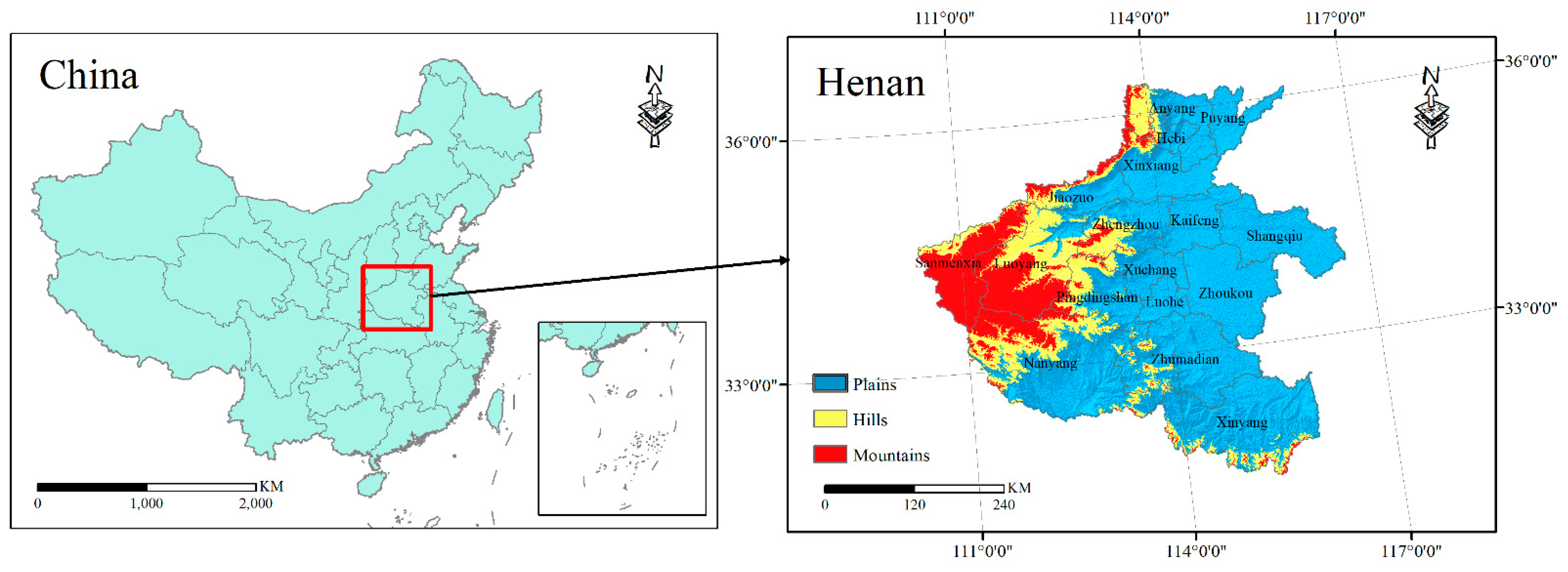
Our study area is Henan province, which is the underdeveloped and largest agricultural province in central China (Figure 1). In 2019, Henan’s total grain output was 66.95 million tons, which is more than one-tenth of China’s total grain output. The agricultural output value was $70.9 billion, and the per capita Gross Domestic Product (GDP) was $8627.30, ranking 3rd and 17th in China, respectively. Henan province has always played the leading role in the formation and development of specialized agricultural villages. Its geography ranges from the mountains in the northwest, west, and south, to the plains in the central and eastern regions. Most of the province is in the warm temperate continental zone, while the southern part has a subtropical continental climate. The average annual temperature, rainfall, and illumination are 10.5–16.7 °C, 407.7–1295.8 mm, and 2000 h. The yearly frost-free period exceeds 250 days [21]. The climatic conditions are helpful for the growth of crops and the development of agriculture.

SAVs data in 2010–2019 were obtained from the Department of Agricultural–Rural Affairs of Henan province. Each record of SAVs contains the name, population, leading industry, total economic product, the number of employees, and per capita disposable income. From these, GP = domestic product, ER = the number of employees/populations of SAV, FI = $\mathrm{per}\mathrm{capita}\mathrm{disposable}\mathrm{income} \ast \mathrm{population}\mathrm{of}\mathrm{SAVs}$. Then, we calculated $\Delta \mathrm{GP}$, $\Delta \mathrm{ER}$, and $\Delta \mathrm{FI}$ of each SAV using Equations (1)–(3), and the proportion of various SAVs in 2011–2014, 2015–2019. Five types of 856 SAVs were selected as research objects since $\Delta \mathrm{GP}$> 0, $\Delta \mathrm{ER}>0$, $\Delta \mathrm{FI}>0$, and each accounted for more than 5% of the total SAVs. Five types of SAVs were shiitakes (37.76%), coarse cereals (21.08%), fruit (12.48%), livestock (11.02%), and Chinese herbal medicine (5.31%), respectively. These SAVs were geocoded with Baidu Maps (the online map servicer of China).

$$\Delta \mathrm{GP}={\mathrm{GP}}_{\mathrm{m}}-{\mathrm{GP}}_{\mathrm{n}}$$

(1)

$$\Delta \mathrm{ER}={\mathrm{ER}}_{\mathrm{m}}-{\mathrm{ER}}_{\mathrm{n}}$$

(2)

$$\Delta \mathrm{FI}={\mathrm{FI}}_{\mathrm{m}}-{\mathrm{FI}}_{\mathrm{n}}$$

(3)

where if m = 2019, n = 2014, else if m = 2014, n = 2010, else if m = 2010,$\Delta \mathrm{GP}={\mathrm{GP}}_{\mathrm{m}}$, $\Delta \mathrm{ER}={\mathrm{ER}}_{\mathrm{m}}$, and $\Delta \mathrm{FI}={\mathrm{FI}}_{\mathrm{m}}$.

The SRTM DEM 30 m data was obtained from the Chinese Academy of Sciences Resource Environment Data Cloud Platform, and it was used to derive the arithmetic mean elevation of SAVs using the zonal statistics as a table tool in ArcGIS 10.7. The window analysis calculated the slope (window size: 2.15 km²) with the SRTM DEM 30 m data. The primary river data of Henan province came from the same platform; it was used to calculate the spatial distance from each SAV to its main river by the near tool available in ArcGIS 10.7. The average annual rainfall data were from the China National Meteorological Data Center to get the average annual rainfall of SAVs. Soil quality data were derived from the land–air interaction research team of Sun Yat-sen University to get the soil quality grade of SAVs. Road network data of Henan province were obtained from the Land Resources Survey and Planning Institute of Henan Province. We used it to calculate the road network distance from each SAV to its county seat, prefecture-level city center, national road, and provincial road. The population, disposable income, and the number of county enterprises were derived from statistical yearbooks.

3. Method

The study presented a data-driven framework to investigate DSAVs and explore the effects of geographical factors. The framework contained four steps: (1) measuring the DSAVs by the construction of SAVDI, (2) quantifying the potential association factors, (3) analyzing the spatial pattern of DSAVs in 2011–2014 and 2015–2019, and (4) evaluating the significantly associated factors and finding the key influencing factor on DSAVs in the SAVs agglomeration regions.

3.1. Measurement of DSAVs

Factor analysis (FA) is a statistical method for extracting common factors from variable groups. This method has been widely used in geography, ecology, and epidemiology. Compared with principal component analysis (PCA), FA better describes the correlation between the original variables [22]. In our study, FA was used to compose the SAVDI to measure the development of each type of SAVs based on three variables—gross product (GP), the employment rate (ER), and farmers’ income (FI). Since there were five main types of SAVs in our study, the SAVDI was further broken down into five indices (see

Table 1. Potential influencing factors on SAVs.

First-Order	Second-Order	Detailed Indicators
Terrain	Elevation	Elevation (T1) *, Mean coefficient of elevation (T2) *, Extreme coefficient of elevation (T3) *
	Slope	Slope (T4) *, Mean coefficient of slope (T5) *, Extreme coefficient of slope (T6) *
Resource	Water resource	Spatial distance from SAVs to river (R1) *, Mean coefficient of spatial distance from SAV to River (R2) *, Extreme coefficient of spatial distance to the river, Rainfall (R3) *, Mean coefficient of rainfall, Extreme value coefficient
	Soil resource	Soil quality grade (R4) *, Mean coefficient, Extreme value coefficient
Location	Distance to city	Spatial distance from SAVs to county (L1) *, Spatial distance from SAV to city
	Traffic accessibility	Network distance from SAVs to road network (L2) *, Mean coefficient of the network distance from SAVs to road network (L3) *, Extreme coefficient of the network distance from SAVs to road network (L4) *
Market	Market scale	County urbanization population (M1) *, Prefecture-level urban population,
	Degree of supply and demand	County urbanization rate (M2) *, Prefecture-level urbanization rate
	Consumption level	Disposable income of urban residents in the county (M3) *
Economy	Total output value	Mean county GDP of former 5 years (E1) *, Mean municipal GDP of former 5 years
	Number of enterprises	The number of agricultural enterprises in the county (E2) *

Note: * indicates the association indicators with VIF no more than 3.

). SAVDI included the specialized shiitake village development index (SSVDI), specialized coarse cereals village development index (SCCVDI), specialized fruit village development index (SFVDI), specialized livestock village development index (SLVDI), and specialized Chinese herbal villages development index (SCVDI). The SAVDI in each period was computed using Equation (4).

$$\mathrm{SAVDI}=\mathrm{a} \ast \left(\mathrm{N}\Delta \mathrm{GP}\right)+\mathrm{b} \ast \left(\mathrm{N}\Delta \mathrm{ER}\right)+\mathrm{c} \ast \left(\mathrm{N}\Delta \mathrm{FI}\right)$$

(4)

where $\mathrm{N}\Delta \mathrm{GP},\mathrm{N}\Delta \mathrm{ER},\mathrm{N}\Delta \mathrm{FI}$ are the normalization results of $\Delta \mathrm{GP}$, $\Delta \mathrm{ER}$, $\Delta \mathrm{FI}$. a, b, and c are the component score coefficients.

3.2. Quantification of the Potential Association Factors

Our study introduced the mean and extreme coefficients to characterize the relative situation of SAVs in its township administrative region. Each township includes many villages in China. Some villages may be SAVs; the number may be 1, 2, or 3. The mean coefficient is the ratio of this specialized agricultural village’s index value to its township administrative area’s average value. The extreme coefficient is the standardized deviation of the index value of SAVs in its township administrative region. The potential influencing indicators (Table 1) were constructed to evaluate the DSAVs from the terrains, resources, locations, markets, and economy. We used elevation, slope, mean, and extreme coefficients to measure terrain, average annual rainfall, and rivers’ spatial distance. Soil grade was used to measure resources. Road network distance and traffic accessibility were utilized to measure economic and transportation characteristics. Market scale, market consumption capacity, and consumption level were used to calculate market characteristics such as supply and demand. GDP and the number of agriculture-related enterprises were used to measure economic development. Then, we assessed the multicollinearity of these variables by analyzing their variance inflation factors (VIF). To ensure that each first-grade index contains the appropriate variables, we used VIF <= 5 as the standard for selecting factors. The results are shown in the * indicators in Table 1, a total of five categories and 11 variables.

According to the potential associated factors in Table 1, we set the independent variables in this study. The independent variables were NT1 = the normalization of mean elevation value (T1) of SAVs, NT4 = the normalization of arithmetic mean slope value (T4) of SAVs. $\mathrm{NR}1=\mathrm{NOR}\left(\mathrm{R}{1}_{\mathrm{i}}-\mathrm{R}{1}_{\mathrm{j}}\right)$, NR3 = the normalization of arithmetic mean rainfall value of SAVs, NR4 = the normalization of arithmetic mean soil quality grade (R4) value of SAVs. $\mathrm{NL}1=\mathrm{NOR}\left(\mathrm{L}{1}_{\mathrm{i}}-\mathrm{L}{1}_{\mathrm{j}}\right)$,$\mathrm{NL}2=\mathrm{NOR}\left(\mathrm{L}{2}_{\mathrm{i}}-\mathrm{L}{2}_{\mathrm{j}}\right)$. $\mathrm{NM}1=\mathrm{NOR}\left(\mathrm{M}{1}_{\mathrm{i}}-\mathrm{M}{1}_{\mathrm{j}}\right)$, $\mathrm{NM}2=\mathrm{M}{2}_{\mathrm{i}}-\mathrm{M}{2}_{\mathrm{j}}$. NE1= the normalization of $\mathrm{E}{1}_{\mathrm{j}}$, $\mathrm{NE}2=\mathrm{NOR}\left(\mathrm{E}{2}_{\mathrm{i}}-\mathrm{E}{2}_{\mathrm{j}}\right)$. Here, $\mathrm{NOR}$ is the normalization function, if i = 2019, j = 2014; when i = 2014, j = 2010.

3.3. Global Moran’s I

Moran’s I is a measure of spatial autocorrelation of DSAVs [23]. Moran’s I test of DSAVs were using $\mathrm{N}\Delta \mathrm{GP}$, $\mathrm{N}\Delta \mathrm{ER}$, $\mathrm{N}\Delta \mathrm{FI}$, and SAVDI by Equations (5) and (6) in this study.

$$\mathrm{I}=\frac{\mathrm{N}{{\displaystyle \sum }}_{\mathrm{i}=1}^{\mathrm{n}}{{\displaystyle \sum }}_{\mathrm{j}=1}^{\mathrm{n}}{\mathrm{W}}_{\mathrm{ij}}\left({\mathrm{x}}_{\mathrm{i}}-{\mathrm{x}}^{\prime }\right)\left({\mathrm{x}}_{\mathrm{j}}-{\mathrm{x}}^{\prime }\right)}{{{\displaystyle \sum }}_{\mathrm{i}=1}^{\mathrm{n}}{{\displaystyle \sum }}_{\mathrm{j}=1}^{\mathrm{n}}{\mathrm{W}}_{\mathrm{ij}}{\left({\mathrm{x}}_{\mathrm{i}}-{\mathrm{x}}^{\prime }\right)}^2}$$

(5)

$$\mathrm{Z}=\frac{\mathrm{I}-\mathrm{E}\left(\mathrm{I}\right)}{\sqrt{\mathrm{VAR}\left(\mathrm{I}\right)}}$$

(6)

where I is the Moran index; n is the number of SAVs; x_i and x_j are the N∆GP, N∆ER, N∆FI, and SAVDI values of ith and jth SAV; ${\mathrm{x}}^{\prime }$ represents the average value of N∆GP, N∆ER, N∆FI, and SAVDI of all SAVs; W_ij is the spatial weight matrix. The spatial weight matrix describes the degree of position association between every two SAVs. W_ij = 1 means that ith and jth SAV are “neighbors”; otherwise, W_ij = 0. The significant differences may appear in the autocorrelation analysis using different spatial weight matrices. I > 0 means positive correlation as a whole; I = 0 means the random distribution; I < 0 means the negative correlation as a whole. VAR(I) is the variance of the global Morin index; E(I) is the expected value of the global Morin index.

3.4. Analyzing the Spatial Pattern of DSAVs

Kernel density estimation is a non-parametric method that uses local information defined by a window (also known as the kernel) to estimate a specified feature’s density at a given location [24]. The kernel density estimation was utilized to analyze the spatial pattern of DSAV by Equations (7)–(9).

$$\hat{\mathrm{f}}\left(\mathrm{x},\mathrm{y}\right)=\frac{1}{{\mathrm{nh}}^2}{\displaystyle \sum }_{\mathrm{i}=1}^{\mathrm{n}}({\mathrm{SAVDI}}_{\mathrm{i}})\mathrm{K}(\frac{{\mathrm{d}}_{\mathrm{i},\left(\mathrm{x},\mathrm{y}\right)}}{\mathrm{h}})$$

(7)

$$\mathrm{K}\left(\frac{{\mathrm{d}}_{\mathrm{i},\left(\mathrm{x},\mathrm{y}\right)}}{\mathrm{h}}\right)=\frac{3}{\mathsf{\pi }}{\left({\left(\frac{{\mathrm{d}}_{\mathrm{i},\left(\mathrm{x},\mathrm{y}\right)}}{\mathrm{h}}\right)}^2\right)}^2$$

(8)

$$\mathrm{h}=\mathsf{\delta }{\left[\underset{-\infty }{\overset{+\infty }{{\displaystyle \int }}}{\mathrm{f}}^{″}{\left({\mathrm{d}}_{\mathrm{i},\left(\mathrm{x},\mathrm{y}\right)}\right)}^2{\mathrm{d}}_{\mathrm{i},\left(\mathrm{x},\mathrm{y}\right)}\right]}^{-0.2}{\mathrm{n}}^{-0.2}$$

(9)

where $\hat{\mathrm{f}}\left(\mathrm{x},\mathrm{y}\right)$ is the density value of the estimated point (x, y); $\mathrm{h}$ represents kernel bandwidth; $\mathrm{n}$ is the sum of $\mathrm{SAVDI}$ within a certain bandwidth range; ${\mathrm{d}}_{\mathrm{i},\left(\mathrm{x},\mathrm{y}\right)}$ is the distance between the event point i and the position (x, y); K is a density function that describes how the contribution of the point i changed with ${\mathrm{d}}_{\mathrm{i},\left(\mathrm{x},\mathrm{y}\right)}$.

3.5. Using Geographic Detectors to Identify the Significant Factors of DSAVs

Geographic Detectors (GDs) are statistical methods that detect spatial differences to reveal the phenomenon’s driving forces. GDs contain 4 detectors (differentiation and factor detection, interaction detection, risk area detection, ecological detection). Compared with traditional classification or partitioning algorithms such as K-means and SOM, the GDs have obvious advantages in spatial differentiation [25]. GDs have been used in land use [26], regional economy [27], public health [28], etc. In this study, we used the differential and factor detector (Equation (10)) to detect the explanatory power of the factors affecting DSAVs. The explanatory power of each factor could be interpreted with the value q. A larger q value indicates that the factor has stronger explanatory power and greater influence on the spatial pattern of DSAVs.

$$\mathrm{q}=1-\frac{{{\displaystyle \sum }}_{\mathrm{h}=1}^{\mathrm{L}}{\mathrm{N}}_{\mathrm{h}}{\mathsf{\sigma }}_{\mathrm{h}}^2}{{\mathrm{N}\mathsf{\sigma }}^2}$$

(10)

where q represents the influencing factor interpretation of DSAVs and ranges from 0 to 1; h is a region (e.g., the prefecture-level village of this study); L is the number of areas of the type; N_h is the number of SAVs in a given area; N is the number of SAVs in the region; ${\mathsf{\sigma }}_{\mathrm{h}}^2$ is the kernel density variance of SAVDI in an SAV; ${\mathsf{\sigma }}^2$ is the kernel density variance of SAVDI throughout regions 1, 2, and 3 in this study.

4. Results

4.1. Spatial Pattern of DSAVs

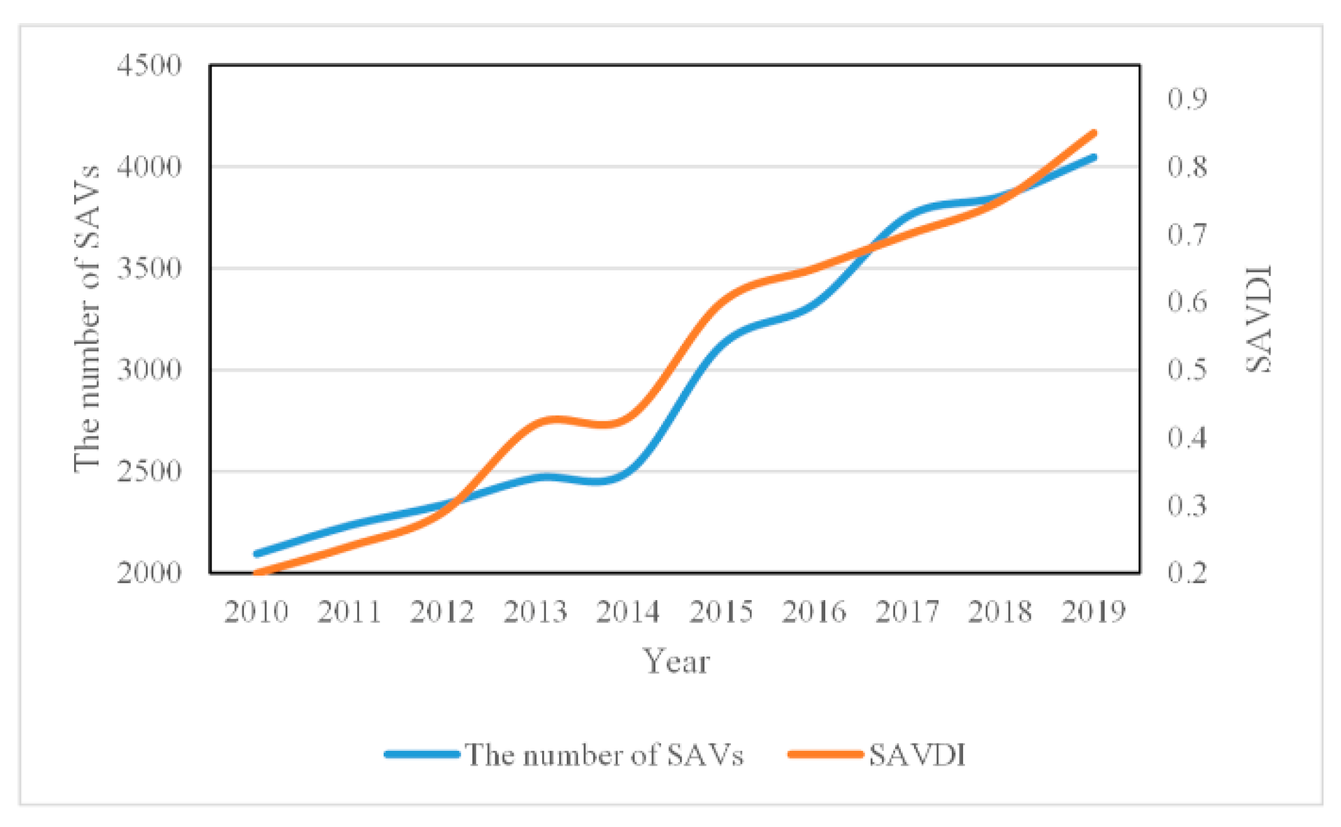
From the changing of the number of SAVs and the value of SAVDI (Section 3.1 for the calculation method) from 2010 to 2019 (Figure 2), this study found that the number of SAVs and the value of SAVDI were an obvious breakpoint in 2014. From 2010 to 2014, the number of SAVs and the value of SAVDI increased relatively flatly over time. After 2014, they have greatly increased from 2015 to 2019. Therefore, this research sets 2011–2014 and 2015–2019 as the periods for this study. The number of SAVs are 2094 (in 2010), 2500 (in 2014), and 4047 (in 2019), respectively.

The results Moran’s I test of DSAVs were using $\mathrm{N}\Delta \mathrm{GP}$, $\mathrm{N}\Delta \mathrm{ER}$, $\mathrm{N}\Delta \mathrm{FI}$, and SAVDI in

Table 2. Moran’s I test of DSAVs.

DSAV.	Global Moran’s I	Z-Value	P-Value
$\mathrm{N}\Delta \mathrm{GP}$	0.47	19.25	0.001
$\mathrm{N}\Delta \mathrm{ER}$	0.51	18.12	0.001
$\mathrm{N}\Delta \mathrm{FI}$	0.49	15.25	0.001
SAVDI	0.45	17.56	0.001

Note: The development of specialized agricultural villages (DSAVs), $\mathrm{N}\Delta \mathrm{GP},\mathrm{N}\Delta \mathrm{ER},\mathrm{and}\mathrm{N}\Delta \mathrm{FI}$ are the normalization results of $\Delta \mathrm{GP}$, $\Delta \mathrm{ER}$, and $\Delta \mathrm{FI}$. $\Delta \mathrm{GP}$, $\Delta \mathrm{ER}$, and $\Delta \mathrm{FI}$ are the changing value of gross product (GP), the employment rate (ER), and farmers’ income (FI) with time for the specialized agriculture village development index (SAVDI).

. Spatial autocorrelation can be observed for all z-values above 15. This finding verified the general consistency derived from SAVDI using multi-source data.

The SAVDI in 2011–2014, 2015–2019 was as the dependent variables and computed by Equation (4) and the component score coefficient matrix of FA in

Table 3. Component score coefficient matrix of factor analysis.

Period of Time	Original Variables	Factors
		SSVDI	SGVDI	SFVDI	SLVDI	SCVDI
2011–2014	$\mathrm{N}\Delta \mathrm{GP}$	0.332	0.258	0.102	0.155	0.752
	$\mathrm{N}\Delta \mathrm{ER}$	0.211	0.554	0.552	0.641	0.341
	$\mathrm{N}\Delta \mathrm{FI}$	0.635	0.285	0.311	0.166	0.156
2015–2019	$\mathrm{N}\Delta \mathrm{GP}$	0.212	0.125	0.158	0.265	0.711
	$\mathrm{N}\Delta \mathrm{ER}$	0.601	0.561	0.441	0.421	0.256
	$\mathrm{N}\Delta \mathrm{FI}$	0.635	0.251	0.321	0.321	0.100

Note: Specialized shiitake village development index (SSVDI), specialized coarse cereals village development index (SCCVDI), specialized fruit village development index (SFVDI), specialized livestock village development index (SLVDI), and specialized Chinese herbal villages development index (SCVDI). $\mathrm{N}\Delta \mathrm{GP},\mathrm{N}\Delta \mathrm{ER},\mathrm{and}\mathrm{N}\Delta \mathrm{FI}$ are the normalization results of $\Delta \mathrm{GP}$, $\Delta \mathrm{ER}$, and $\Delta \mathrm{FI}$. $\Delta \mathrm{GP}$, $\Delta \mathrm{ER}$, and $\Delta \mathrm{FI}$ are the changing value of gross product (GP), the employment rate (ER), and farmers’ income (FI) with time.

. Here, when we calculated SSVDI in 2011–2014, a = 0.332, b= 0.211, and c = 0.635 in Equation (4). By analogy, we used the same scheme to calculate the SCCVDI, SFVDI, SLVDI, and SCVDI in 2011–2014, 2015–2019, respectively.

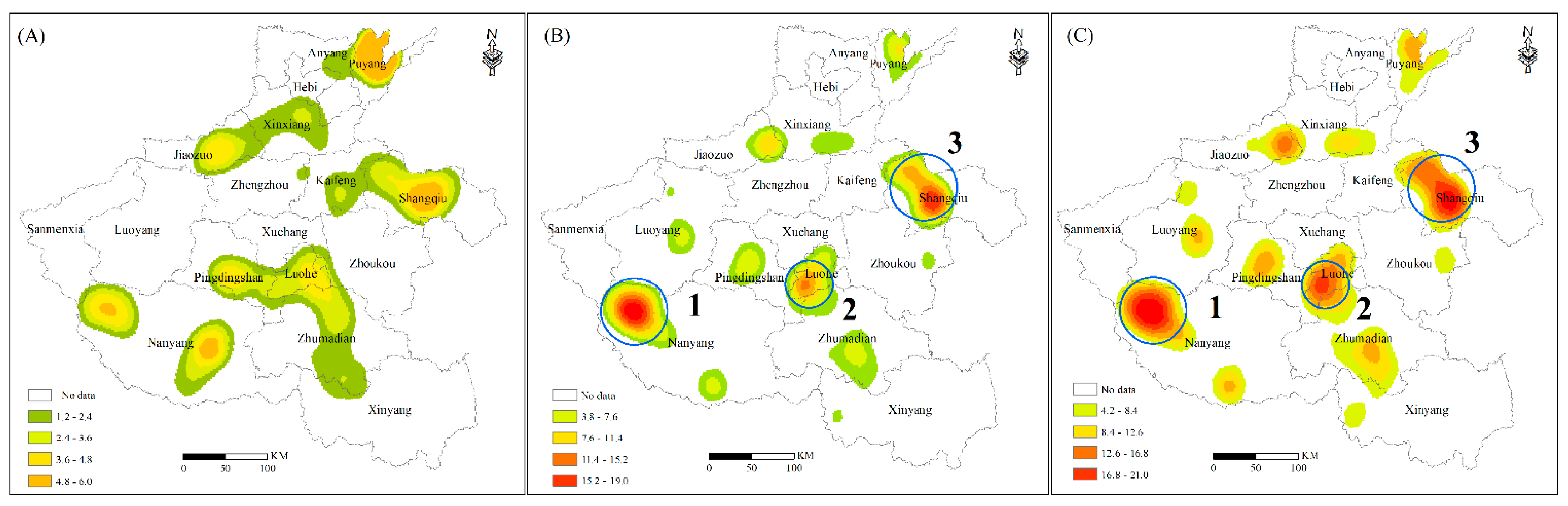
The results of the kernel density analysis of SAVDI are shown in Figure 3. We found that SAVs were unevenly distributed in 2010 (Figure 3A), and the degree of aggregation increased from 2010 to 2019 (Figure 3B,C). The agglomeration of SAVs concentrated in the province’s marginal area and then enhanced in the periphery of Luohe (Figure 3). The kernel density values were above 10.0 pcs/10,000 km² in the western Nanyang (region 1), Luohe (region 2), and northwestern Shangqiu (region 3) from 2010 to 2014 (Figure 3B). The SAVs clustered in Luohe, Puyang, Jiaozuo, northwestern Shangqiu, and western Nanyang from 2015 to 2019, and the kernel density values were over 13 pcs/10,000 km² (Figure 3C). In these two time periods, region 1 (mountain–plain area), region 2 (hill–plain area), and region 3 (plain area) are areas where hot spots of SAVs persisted, but their development capabilities are different. Specifically, the accumulation of specialized shiitake villages was in region 1. The kernel density values were above 12.0 (in 2011–2014) and 15.0 (in 2015–2019). Specialized coarse cereals villages clustered in region 2 from 2010 to 2019. Specialized fruit and livestock villages were growing in region 3 from 2010 to 2019. Specialized Chinese herbal villages agglomerated in region 1, and the kernel density value was increasing from 2010 to 2019.

4.2. Identifying the Key Influencing Factors of DSAVs

The DSAVs were affected by multiple factors. With the elimination of numerous co-linear effects, influencing factors ended up with 11 indicators in five categories: terrain, resources, location, market, and economy. As illustrated in

Table 4. Geographical detector analysis results of the impact factors of SVAD.

Indicator	SAVDI (2011–2014)		SAVDI (2015–2019)
	q Statistic	p Value	q Statistic	p Value
T1	0.1311	0.0000	0.1012	0.0000
T4	0.3158	0.0000	0.1581	0.0000
R1	0.1521	0.0000	0.0325	0.0311
R3	0.1112	0.0000	-	-
R4	-	-	0.0125	0.0221
L1	0.4120	0.0000	0.1251	0.0000
L2	0.1985	0.0000	-	-
M1	0.1421	0.0000	0.3814	0.0000
M2	0.1025	0.0000	0.1528	0.0000
M3	0.0211	0.0325	0.1645	0.0000
E1	-	-	0.4021	0.0000
E2	0.0112	0.0412	0.1514	0.0000

Note: T1: elevation value, T4: slope, R1: the spatial distance from SAV to river, R3: rainfall, R4: soil quality grade, L1: the spatial distance from SAV to county, L2: the spatial distance from SAV to road network, M1: county urbanization population, M2: county urbanization rate, M3: disposable income of urban residents in the county, E1: mean county GDP of former 5 years; E2: the number of agricultural enterprises in the county.

, most of the indicators had significant (p < 0.01) impacts on DSAVs in the SAVs agglomeration regions 1, 2, and 3. Terrain and location factors were the key influencing factors in 2011–2014; economic and market factors were the key factors in 2015–2019.

Geographical detector analysis results in region 1 (

Table 5. Geographical detector analysis results of the impact factors of the development of specialized shiitake villages in region 1.

Indicator	SSVDI (2011–2014)		SSVDI (2015–2019)
	q Statistic	p Value	q Statistic	p Value
T1	0.1211	0.0000	0.1010	0.0000
T4	0.1158	0.0000	0.1147	0.0000
R1	0.1521	0.0000	0.1245	0.0000
R3	0.1011	0.0000	-	-
R4	-	-	-	-
L1	0.1623	0.0000	0.1058	0.0000
L2	0.4712	0.0000	0.0812	0.0301
M1	0.1371	0.0000	0.1821	0.0000
M2	0.1125	0.0000	0.1258	0.0000
M3	-	-	0.4513	0.0000
E1	0.1123	0.0000	0.1122	0.0000
E2	0.1128	0.0000	0.2115	0.0000

and

Table 6. Geographical detector analysis results of the impact factors of the development of specialized Chinese herbal medicine villages in region 1.

Indicator	SCVDI (2011–2014)		SCVDI (2015–2019)
	q Statistic	p Value	q Statistic	p Value
T1	0.2211	0.0000	0.1561	0.0000
T4	0.1350	0.0000	0.1012	0.0000
R1	0.0121	0.0000	0.0000	0.0000
R3	0.0011	0.0000	-	-
R4	-	-	0.0320	0.0221
L1	0.1214	0.0000	0.0058	0.0311
L2	0.1104	0.0000	0.1012	0.0000
M1	0.0121	0.0111	0.0032	0.0124
M2	0.0352	0.0344	0.1058	0.0000
M3	0.0214	0.0221	0.0522	0.0000
E1	0.1251	0.0000	0.2136	0.0000
E2	0.3258	0.0000	0.4125	0.0000

Note: Specialized shiitake village development index (SSVDI), specialized Chinese herbal villages development index (SCVDI); T1: elevation value, T4: slope, R1: the spatial distance from SAV to river, R3: rainfall, R4: soil quality grade, L1: the spatial distance from SAV to county, L2: the spatial distance from SAV to road network, M1: county urbanization population, M2: county urbanization rate, M3: disposable income of urban residents in the county, E1: mean county GDP of former 5 years; E2: the number of agricultural enterprises in the county.

) showed that the development of specialized shiitake villages was mainly affected by the distances of SAVs to the road network (q statistic = 0.4712, p < 0.01), the spatial distance to the county (q statistic = 0.1623, p < 0.01) in 2011–2014; the disposable income of urban residents in the county (q statistic = 0.4513, p <0.01), and the number of agricultural enterprises in the county (q statistic = 0.2115, p < 0.01) from 2015 to 2019. The development of specialized Chinese herbal medicine villages was affected by the number of agricultural enterprises of the county in 2011–2014 and 2015–2019 (q statistic = 0.3258 and 0.4125, respectively, p <0.01).

In region 2, the development of specialized coarse cereals villages (

Table 7. Geographical detector analysis results of the impact factors of the development of specialized coarse cereals villages in region 2.

Indicator	SCCVDI (2011–2014)		SCCVDI (2015–2019)
	q Statistic	p Value	q Statistic	p Value
T1	0.1444	0.0000	0.1015	0.0000
T4	0.1026	0.0000	0.1145	0.0000
R1	0.2521	0.0365	0.0056	0.0311
R3	0.1147	0.0000	0.0651	0.0452
R4	0.1256	0.000	-	-
L1	0.3521	0.0000	0.4114	0.0000
L2	0.1099	0.0000	0.1789	0.0000
M1	0.0547	0.0211	0.3796	0.0000
M2	0.0158	0.0355	0.1485	0.0000
M3	-	-	0.1254	0.0000
E1	-	-	0.4388	0.0000
E2	0.1125	0.0000	0.2411	0.0000

Note: Specialized coarse cereals village development index (SCCVDI); T1: elevation value, T4: slope, R1: the spatial distance from SAV to river, R3: rainfall, R4: soil quality grade, L1: the spatial distance from SAV to county, L2: the spatial distance from SAV to road network, M1: county urbanization population, M2: county urbanization rate, M3: disposable income of urban residents in the county, E1: mean county GDP of former 5 years; E2: the number of agricultural enterprises in the county.

) was impacted by the spatial distance from SAV to the county (q statistic = 0.3521, p < 0.01) in 2011–2014, and 2015–2019 (q statistic = 0.4114, p < 0.01), which was followed by the spatial distance from SAVs to a river in 2011–2014 (q statistic = 0.2521, p < 0.01) and the number of agricultural enterprises in the county in 2015–2019 (q statistic = 0.2411, p < 0.01).

In region 3 (

Table 8. Geographical detector analysis results of the impact factors of the development of specialized fruit villages in region 3.

Indicator	SFVDI (2011–2014)		SFVDI (2015–2019)
	q Statistic	p Value	q Statistic	p Value
T1	0.0325	0.0362	0.0025	0.0488
T4	0.0012	0.0500	0.0204	0.0362
R1	0.2111	0.0000	0.1145	0.0000
R3	0.1525	0.0000	0.1741	0.0000
R4	0.2855	0.0000	0.1401	0.0000
L1	0.1117	0.0000	-	-
L2	0.1109	0.0000	0.1789	0.0000
M1	0.0547	0.0311	-	-
M2	0.1425	0.0000	0.1811	0.0000
M3	0.1845	0.0000	0.3477	0.0000
E1	-	-	0.1201	0.0000
E2	0.1114	0.0000	0.1000	0.0000

and

Table 9. Geographical detector analysis results of the impact factors of specialized livestock villages’ development.

Indicator	SAVDI (2011–2014)		SAVDI (2015–2019)
	q Statistic	p Value	q Statistic	p Value
T1	-	-	-	-
T4	-	-	-	-
R1	0.0045	0.0211	0.1156	0.0359
R3	-	-	-	-
R4	-	-	-	-
L1	0.1147	0.0000	0.1341	0.0000
L2	0.3250	0.0000	0.1658	0.0000
M1	0.1166	0.0000	0.1230	0.0000
M2	0.1014	0.0000	0.1552	0.0000
M3	0.1254	0.0000	0.3125	0.0000
E1	0.1030	0.0000	0.1311	0.0000
E2	0.1141	0.0000	0.1115	0.0000

Note: Specialized fruit village development index (SFVDI), specialized livestock village development index (SLVDI); T1: elevation value, T4: slope, R1: the spatial distance from SAV to a river, R3: rainfall, R4: soil quality grade, L1: the spatial distance from SAV to the county, L2: the spatial distance from SAV to the road network, M1: county urbanization population, M2: county urbanization rate, M3: disposable income of urban residents in the county, E1: mean county GDP of former 5 years; E2: the number of agricultural enterprises in the county.

), the largest influence factors of the development of specialized fruit villages were soil quality (q statistic = 0.2855, p < 0.01) and the disposable income of urban residents in the county (q statistic = 0.3477, p < 0.01) for 2011–2014 and 2015–2019, respectively. The second largest influence factors of the development of specialized fruit villages were the spatial distances to rivers (q statistic = 0.2111, p < 0.01) and county urbanization rate (q statistic = 0.1811, p < 0.01) in 2011–2014 and 2015–2019, respectively. Specialized livestock villages’ development was mainly influenced by the spatial distances from villages to the road network in 2011–2014 (q statistic = 0.3250, p < 0.01). This pattern changed in 2015–2019; the key factor become the disposable income of urban residents in the county in 2015–2019 (q statistic = 0.3125, p < 0.01).

5. Discussion

Studies show that the SAVs in Henan province began to form in the late 2000s and saw the steady growth in the early 2010s [2]. It was not until later that decade, when the national government diverted more attention and resources to rural development that these SAVs flourished unprecedently [15]. The average and extreme coefficients of the influencing factors of SAVs have remained stable. The average coefficients of various indicators fluctuated around 0.8, and the extreme coefficients fluctuated around 0.2 in 2010 (

Table 10. Statistical mean and extreme coefficient of influencing factors of SAVs (2010).

Indicator	Shiitake	Coarse Cereals	Fruit	Livestock	Chinese Herbal Medicine
T2	0.84	0.85	0.8	0.94	0.83
T3	0.2	0.22	0.18	0.21	0.19
T5	0.75	0.73	0.83	0.82	0.81
T6	0.16	0.18	0.2	0.22	0.23
R2	0.85	0.91	0.88	1.03	0.93
L3	0.78	0.72	0.79	0.8	0.77
L4	0.19	0.21	0.21	0.20	0.23

Note: T2: mean coefficient of elevation, T4: slope, T3: Extreme coefficient of elevation, T5: mean coefficient of slope, T6: the extreme coefficient of slope, R2: mean coefficient of spatial distance from SAV to river, L3: mean coefficient of the network distance from SAVs to road network, L4: extreme coefficient of the network distance from SAVs to road network.

). SAVs converged toward regions that were relatively superior in terms of terrains, resources, and locations. However, with the improving infrastructure such as roads, rail, etc., the influencing factors on DSAVs were also changing. Compared with 2010 (during the initial stage of SAVs’ formation), the importance of terrain and location factors to SAVs decreased, while the importance of market and economic factors was increasing in 2011–2014 and 2015–2019. Market and economic factors became the key factors affecting DSAVs in Henan.

The fact that the market and economic factors gradually became more critical overtime was in line with previous research on the development of rural areas at the township level [29]. With the economy’s improvement, traditional geographical factors such as topography, resources, and location on economic development in agricultural regions have gradually decreased, and geographical proximity became a significant driver of economic accumulation. The importance of economic factors has steadily increased. The similarity of the findings indicates that the DSAVs at the township level or the village level and economic activities other than agriculture have gradually increased, and the importance of economic development factors has also increased.

While research pointed to market demand as the only factors affecting SAVs in China’s northern plain–hill areas [4], it was for a specific time (in 2011 or 2017). Thus, it focuses on a particular section in DSAVs. However, our study of Henan province, which is also dominated by plains and hilly areas (more than 60%), points to a gradual but steady shift of importance from topography, resources to market, and economic factors. This reveals the long-term development pattern of SAVs and their changing trends at the macro time scale.

As location factors had become less important and were slowly eclipsed by market and resource factors in the development of specialized shiitake and fruit villages, we could consider relocating and merging them with small-scale underdeveloped villages. In doing so, we tap into the high-value agricultural products in a planned way. Similarly, the importance of location and resource factors to specialized coarse cereals, livestock, and Chinese herbal medicine villages was slowly surpassed by market and economic factors. The continued development of these SAVs requires that measures be taken, including in-depth analysis of the agricultural product markets, improving the quality of agricultural products, establishing smooth transportation channels for markets, etc.

Even though the key influencing factors of the development of various SAVs were similar, their respective importance was quite different. A case in point is the key factors influencing the development of specialized shiitake and fruit villages. While both were market elements, the explanatory powers and specific indicators were different. The disposable income of urban residents in the county was the key factor for specialized shiitake villages in 2015–2019 (q statistic = 0.4642, p < 0.01), while for specialized fruit villages, the driving factor was the county urbanization population in 2015–2019 (q statistic = 0.3275, p < 0.05). Therefore, when guiding the DSAVs, relevant authorities need to pay attention to the importance of the factors affecting DSAVs and the differences brought forward by change of the village types to realize the refined guidance for DSAVs.

6. Conclusions

The geographical factors play an essential role in the development of SAVs in undeveloped regions in China. However, perhaps simply due to a lack of long-term data of SAVs, few studies focused on the continued development of SAVs over a longer temporal scale. Responding to this deficiency, we integrated multi-source data, applied the geographic detector and other methods to analyze the spatial pattern of SAVs, and explored DSAVs as affected by the geographical environment in Henan Province, China. The main conclusions are as follows. (1) The spatial pattern of DSAVs presented the characteristics of aggregation in the marginal area of the provincial boundary and the significantly growing cluster in the western Nanyang (mountain), Luohe (hill–plain), and northwestern Shangqiu (plain). (2) The importance of terrain and transportation to DSAVs is decreasing, while the importance of market and economy is increasing. (3) According to the explanatory power changing of influencing factors of various SAVs in the different regions, the strongest changing was specialized shiitake villages in the western Nanyang (mountain region).

DSAVs is often affected by multiple factors, such as rural elites and rural self-development capabilities. However, it is challenging to find indicators that reflect the emergence of rural elites, rural self-development capabilities, and other factors in this research. One possible solution is to introduce new data and indicator systems to look at potential factors (e.g., availability of skilled labor, ready supply of inputs, climate change, risks and export markets) in future research. This will support decision making for the underdeveloped areas to formulate rural development strategies tailored to local conditions.

References

- Liu, Y.; Li, Y. Revitalize the world’s countryside. Nature 2018, 548, 275–277. [Google Scholar] [CrossRef]
- Li, X.; Zhou, X.; Zheng, C.; Scott, R. Development of Specialized Villages in Various Environments of Less Developed China. Acta Geogr. Sin. 2012, 67, 783–792. (In Chinese) [Google Scholar]
- Bellandi, M.; Di Tommaso, M.R. The case of specialized towns in Guangdong, China. Eur. Plan. Stud. 2005, 13, 707–729. [Google Scholar] [CrossRef]
- Cao, Z.; Liu, Y.; Li, Y.; Wang, Y. Spatial pattern and its influencing factors of specialized villages and towns in China. Acta Geogr. Sin. 2020, 75, 1647–1666. (In Chinese) [Google Scholar]
- MARAC. Reply to Recommendation No. 3421 of the Fifth Session of the Twelfth National People’s Congress. Available online: http://www.moa.gov.cn/gk/jyta/201710/t20171017_5842497.htm (accessed on 18 October 2017).
- Omamo, S.W. Farm to market transaction costs and specialisation in small scale agriculture: Explorations with a non-separable household model. J. Dev. Stud. 1998, 35, 152–163. [Google Scholar] [CrossRef]
- Leaman, J.H.; Conkling, E.C. Transport change and agricultural specialization. Ann. Assoc. Am. Geogr. 1975, 65, 425–432. [Google Scholar] [CrossRef]
- Pachoud, C.; Delay, E.; Re, R.D.; Ramanzin, M.; Sturaro, E. A relational approach to studying collective action in dairy cooperatives producing mountain cheeses in the Alps: The case of the primiero cooperative in the eastern Italians Alps. Sustainability 2020, 12, 4596. [Google Scholar] [CrossRef]
- De Roest, K.; Ferrari, P.; Knickel, K. Specialisation and economies of scale or diversification and economies of scope? Assessing different agricultural development pathways. J. Rural Stud. 2017, 59, 222–231. [Google Scholar] [CrossRef]
- Emran, M.S.; Shilpi, F. The Extent of the Market and Stages of Agricultural Specialization; The World Bank: Washington, DC, USA, 2008; pp. 1123–1126. [Google Scholar]
- Mora, R.; San Juan, C. Geographical specialisation in Spanish agriculture before and after integration in the European Union. Reg. Sci. Urban. Econ. 2004, 34, 309–320. [Google Scholar] [CrossRef] [Green Version]
- Li, Y.; Fan, P.; Liu, Y. What makes better village development in traditional agricultural areas of China? Evidence from long-term observation of typical villages. Habitat. Int. 2019, 83, 111–124. [Google Scholar] [CrossRef]
- Chen, G.; Hamori, S. Rural Labor Migration, Discrimination, and the New Dual Labor Market in China; Springer Science & Business Media: Berlin, Germany, 2013; pp. 154–196. [Google Scholar]
- Li, X.; Ye, X.; Zhou, X.; Zheng, C.; Leipnik, M.; Lou, F. Specialized villages in inland China: Spatial and developmental issues. Sustainability 2018, 10, 2994. [Google Scholar] [CrossRef] [Green Version]
- Gao, G.; Shi, L. The formation process of specialized village and its influence factors-a case study for three sample villages in the southwest of Henan province. Econ. Geogr. 2011, 31, 1165–1170. (In Chinese) [Google Scholar]
- Qiao, J.; Lee, J.; Ye, X. Spatiotemporal evolution of specialized villages and rural development: A case study of Henan province, China. Ann. Am. Assoc. Geogr. 2016, 106, 57–75. [Google Scholar] [CrossRef]
- Wu, N.; Li, E.; Li, X. Spatial distribution of specialized vegetable cultivation villages and its influencing factors: A case study of capsicum plantation in Zhecheng County, Henan Province. Geogr. Res. 2013, 32, 1303. (In Chinese) [Google Scholar]
- Wu, N.; Li, L.; Li, E.; Li, X. The Spatial Continuity of Specialized Plantation: A Case Study of Raspberry Farm in Fengqiu County, Henan Province. Sci. Geogr. Sin. 2018, 38, 428–436. (In Chinese) [Google Scholar]
- Liu, Y.; Lu, S.; Chen, Y. Spatio-temporal change of urban–rural equalized development patterns in China and its driving factors. J. Rural Stud. 2013, 32, 320–330. [Google Scholar] [CrossRef]
- Ngugi, J.; Bwisa, H. Factors influencing growth of group owned small and medium enterprises: A case of one village one product enterprises. Int. Educ. Res. J. 2013, 1, 1–14. [Google Scholar]
- Liu, S.; Qin, Y.; Xu, Y. Inequality and influencing factors of spatial accessibility of medical facilities in rural areas of China: A case study of Henan province. Int. J. Environ. Res. Public Health 2019, 16, 1833. [Google Scholar] [CrossRef] [PubMed] [Green Version]
- Gudjonsson, G. An easy guide to factor analysis. Personal. Individ. Differ. 1994, 17, 302. [Google Scholar] [CrossRef]
- Moran, P.A. Notes on continuous stochastic phenomena. Biometrika 1950, 37, 17–23. [Google Scholar] [CrossRef] [PubMed]
- Shi, X. Selection of bandwidth type and adjustment side in kernel density estimation over inhomogeneous backgrounds. Int. J. Geogr. Inf. Sci. 2010, 24, 643–660. [Google Scholar] [CrossRef]
- Wang, J.; Li, X.; Christakos, G.; Liao, Y.; Zhang, T.; Gu, X.; Zheng, X. Geographical detectors-based health risk assessment and its application in the neural tube defects study of the Heshun region, China. Int. J. Geogr. Inf. Sci. 2010, 24, 107–127. [Google Scholar] [CrossRef]
- Ju, H.; Zhang, Z.; Zuo, L.; Wang, J.; Zhang, S.; Wang, X.; Zhao, X. Driving forces and their interactions of built-up land expansion based on the geographical detector—A case study of Beijing, China. Int. J. Geogr. Inf. Sci. 2016, 30, 2188–2207. [Google Scholar] [CrossRef]
- Zhao, Y.; Deng, Q.; Lin, Q.; Cai, C. Quantitative analysis of the impacts of terrestrial environmental factors on precipitation variation over the Beibu gulf economic zone in coastal southwest China. Sci. Rep. 2017, 7, 44412. [Google Scholar] [CrossRef] [PubMed]
- Liao, Y.; Wang, J.; Du, W.; Gao, B.; Liu, X.; Chen, G.; Song, X.; Zheng, X. Using spatial analysis to understand the spatial heterogeneity of disability employment in China. Trans. GIS 2017, 21, 647–660. [Google Scholar] [CrossRef]
- Li, X.; Zhou, X.; Zheng, C. Geography and Economic Development in Rural China: A Township Level Study in Henan Province, China. Acta Geogr. Sin. 2008, 63, 147–155. (In Chinese) [Google Scholar]
Figure 1.
The case study area: Henan, China.
Figure 2.
The number of SAVs and the value of SAVDI from 2010 to 2019.