
Land Cover Mapping from Colorized CORONA Archived Greyscale Satellite Data and Feature Extraction Classification


1
Department of Civil Engineering and Geomatics, Faculty of Engineering and Technology, Cyprus University of Technology, Saripolou 2-8, Limassol 3036, Cyprus
2
Eratosthenes Centre of Excellence, Saripolou 2-8, Limassol 3036, Cyprus
Land 2021, 10(8), 771; https://0-doi-org.brum.beds.ac.uk/10.3390/land10080771
Submission received: 25 June 2021
/
Revised: 18 July 2021
/
Accepted: 21 July 2021
/
Published: 22 July 2021
(This article belongs to the Special Issue Geomatics for Resource Monitoring and Management)
Abstract
:Land cover mapping is often performed via satellite or aerial multispectral/hyperspectral datasets. This paper explores new potentials for the characterisation of land cover from archive greyscale satellite sources by using classification analysis of colourised images. In particular, a CORONA satellite image over Larnaca city in Cyprus was used for this study. The DeOldify Deep learning method embedded in the MyHeritage platform was initially applied to colourise the CORONA image. The new image was then compared against the original greyscale image across various quality metric methods. Then, the geometric correction of the CORONA coloured image was performed using common ground control points taken for aerial images. Later a segmentation process of the image was completed, while segments were selected and characterised for training purposes during the classification process. The latest was performed using the support vector machine (SVM) classifier. Five main land cover classes were selected: land, water, salt lake, vegetation, and urban areas. The overall results of the classification process were then evaluated. The results were very promising (>85 classification accuracy, 0.91 kappa coefficient). The outcomes show that this method can be implemented in any archive greyscale satellite or aerial image to characterise preview landscapes. These results are improved compared to other methods, such as using texture filters.
Keywords:
historical land cover; CORONA; feature extraction; classification; MyHeritage; deep learning; Cyprus1. Introduction
Land cover mapping is considered one of the most well-documented research areas of remote sensing science [1,2]. Numerous applications have been presented in the past dealing with this topic [3,4,5,6]. The majority of these studies focus on the exploitation of multispectral and hyperspectral data sets to generate land cover maps [7,8,9,10]. At the end of a classification process, the satellite image is labelled into the pre-defined thematic land use classes, while the overall results are evaluated via different classification metrics. In an attempt to improve the overall results, the classification process has been shifted from pixel-based to object-oriented and segmentation analysis during recent years [11,12,13].
Land cover maps are considered essential for studying diachronic landscape changes that can promote sustainability. Indeed, land cover analysis is fundamental for a wide range of applications like ecology, environment, agriculture, transport, spatial planning, and others. The conversion of land cover to artificial cover can lead to many environmental issues, including land surface temperature [14], loss of ecosystem services, urbanisation, changes in water yields, or habitat degradation. Analysis of time-series land cover maps can provide details for land cover dynamics [15], land-use emissions [16], urban extent [17], and artificially impervious areas [18]. In addition, land cover maps can be used for monitoring natural hazards like floods and soil erosion. For instance, [19] used Landsat images to deliver land cover maps to characterise the 2014 flood of the Indus River in Pakistan. Moreover, land use maps generated from satellite images were used for flood monitoring in the area of Yialias in Cyprus [20]. Land cover maps obtained from space sensors have also been used in soil erosion studies [21].
The CORINE Land Cover (CLC) inventory is considered one of the earliest databases at the European level delivering land cover maps. CLC was created to standardise data collection related to land in Europe to support environmental policy development. It was initiated in 1985 (with the reference year of 1990) and continues until today to characterise the various thematic classes at a European level. CLC updates have been produced in 2000, 2006, 2012, and 2018 [22,23].
Scientists today have access to a variety of high-resolution satellite imagery, like the WorldView sensor with a special resolution of up to 30 centimetres. However, these images became available during the last two decades, after the launch of the IKONOS sensor, the first commercial satellite sensor in 1999. Before that period, scientists could work with medium resolution satellite data with a spatial resolution between 10 to 30 through the Landsat space program (since 1972) and the Satellite pour l’Observation de la Terre (SPOT) sensor in the 1980s.
During the 1960s and 70s, available information from intelligence satellite sensors could be accessed through other space programmes, like those of the CORONA sensor. The specific images were initially used for reconnaissance purposes and to produce maps for US intelligence agencies. In 1992, an Environmental Task Force evaluated the application of early satellite data for environmental studies, and the images were declassified by Executive Order 12,951 in 1995 [24].
The use of CORONA archive images and other similar datasets for producing historical land cover maps has already been presented in the literature [25,26,27,28]. In [29], the researchers used aerial photographs from 1944 to map agricultural lands and forests, while CORONA satellite images were used to map agricultural lands following an object-based image analysis (OBIA). In [30], the authors proposed an image texture derived method to characterise historical land cover from CORONA data. Other studies have used the CORONA datasets for land cover analysis using classification image processing techniques [31], density slicing [32], as well as image interpretation and digitisation [33]. Recently, Deshpande et al. [34] have worked with convolutional neural networks (2D-CNN) and texture extraction obtained through geometric moments (GM) to produce classification results from greyscale CORONA images. In addition, an effort to improve the interpretation of CORONA images, for archaeo-landscape studies, by adding colour from recently acquired satellites or airborne sensors was presented by [35].
This paper aims to present a methodology where historical land cover maps can be retrieved from CORONA imagery using deep learning colourisation techniques, feature extraction, and vector machine classification. An example of this proposed methodology is presented here using a medium resolution CORONA image from 1963. The overall assumptions, evaluation metrics, and results are presented below.
2. Materials and Methods
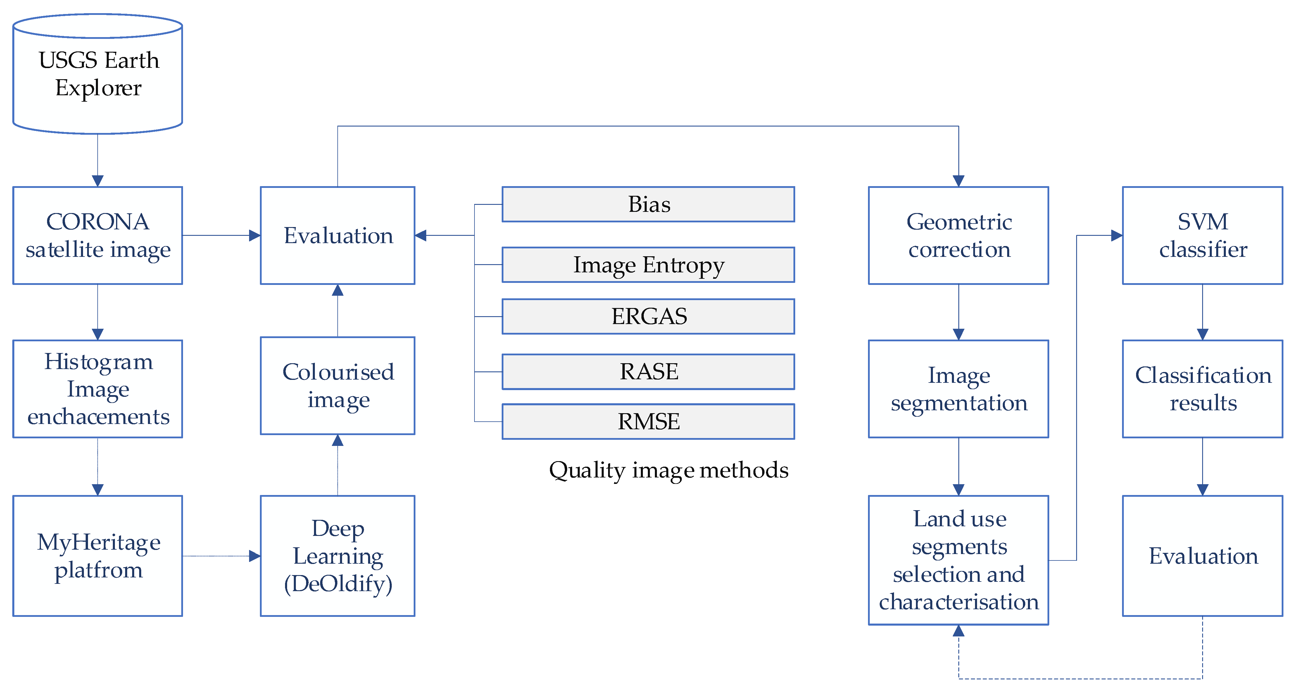
The overall methodology followed in this study is presented in Figure 1. Initially, a CORONA greyscale image was downloaded from the USGS Earth Explorer platform [36]. The CORONA image with Entity ID DS009056009DA077 and coordinates 35.080, 34.067 (WGS 84 geodetic system) was chosen. The image covers Larnaca city in Cyprus, while the acquisition date was 27 June 1963. The CORONA mission number was 9056, using the KH-4 mission designator and a 70 mm panoramic film type. The resolution of the image is estimated to be 25 feet (equivalent of 7.62 m).
After the image was downloaded, an image enhancement using histogram linear stretching techniques (2%) was applied to improve the image interpretation and quality of the original image. Then, a selection (subset) of the image covering the area of interest over Larnaca city was made. This subset was uploaded to the MyHeritage in ColorTM platform [37] for colourising purposes. The specific platform has licensed the DeOldify deep learning model [38] exclusively, using an improved version of the generative adversarial networks (GANs). This pre-defined model was trained using millions of real photos and could colourise greyscale photos [37]. Various other examples from this process can be found on the MyHeritage in ColorTM platform website [37]. The original code of the DeOldify deep learning model can be accessed from [38].
It should be mentioned that the final colourisation image remains a simulation, and consequently, an evaluation of the final output is needed. We have therefore compared the original CORONA image with the colourised one using different quality image metrics. Specifically, we have explored five different quality metrics as follow (see Equations (1) to (5)):
The Bias method estimates the deviation degree between the colourised and the original CORONA image, while Image Entropy quantifies the information of the colourised image based on the Shanon theorem. The ERGAS (erreur relative globale adimensionnelle de synthèse) estimates the ratio between pixels of the colourised and the original CORONA image. The RASE (relative average spectral error) method characterises the average performance of the colourised image, and finally, the RMSE (root mean squared error) method measures the difference between the reference image and the colourised image. More details regarding these quality image methods can be found in [39,40]. These quality methods were implemented in the MathWorks MATLAB R2016b environment based on [40] toolbox.
Once the above evaluation had been performed, a geometric correction of the colourised image was carried out using a second-order polynomial model. Fifteen ground control points were used, uniformly scattered over the case study for the geometric transformation, using a high-resolution aerial orthophoto image as reference. The aerial dataset was obtained from the same period as the CORONA images (1963) and was provided by the Department of Land and Surveyors (as WMS service). The accuracy of the reference images is estimated to be 1.25 m (scale 1: 5000), which is sufficient for the CORONA correction (pixel size 7.62 m). The geometric correction was applied in the ArcGIS v10.2 environment (ESRI).
The next step included the classification of the colourised image using training samples. The colourised image is composed of three spectral bands, namely the blue, green, and red (compared with a single spectral layer of the original CORONA image). Therefore, different supervised classification techniques can be applied. In this study, we explored the potentials of the object-oriented classification through the segmentation of the image and the classification strategy using the support vector machine (SVM) classifier, as this was found to be promising in other relevant studies [14]. Training samples after the interpretation of the CORONA image were used for classification purposes.
The SVM classifier is a supervised classification approach developed from a statistical learning theory. SVM is capable of modelling nonlinear connections while avoiding overfitting through regularisation [41,42,43,44]. The classifier separates the various classes with a decision surface (optimal hyperplane) that maximises the margin between the classes. Here, the radial basis function (RBF) kernel function was used to estimate the weights of nearby data points in estimating target classes (Equation (6)). The degree of the kernel polynomial was set to 1, while the Gamma parameter (g) was set to 0.03. Finally, the penalty parameter was set to 100.
RBF = K(xi,xj) = exp(−g||xi − xj||2), g > 0
This classification process was repeated (e.g., including new training samples) to improve the classifier’s overall performance. Finally, the land cover map was produced with the following five thematic classes: land, water, salt lake, vegetation, and urban areas. The overall results were then evaluated using the error matrix and classification metrics accuracy. The following three metrics were used: (a) the overall accuracy, which is calculated by summing the number of correctly classified values and dividing by the total number of values (see Equation (7)); (b) the accuracy per class, which is the percentage of the corrected classified pixels divided by the total number of the correct pixels in this class (see Equation (8)), and (c) Kappa coefficient that measures the agreement between classification and truth values. A kappa value of 1 represents perfect agreement, while a value of 0 represents no agreement (see Equation (9))
where i is the class number, N is the total number of classified values compared to truth values, mi,i is the number of values belonging to the truth class i that have also been classified as class i, Ci is the total number of predicted values belonging to class i, and Gi is the total number of truth values belonging to class i.
3. Results
3.1. Colourisation of the CORONA Image
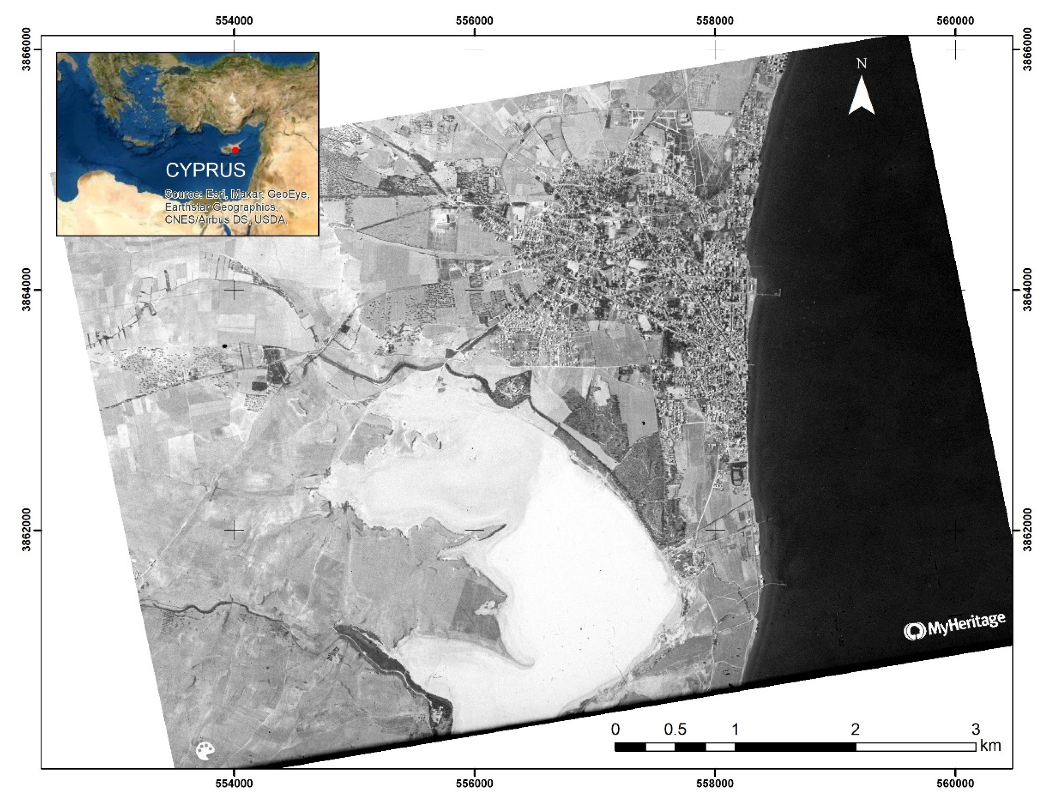
Figure 2 shows the initial CORONA greyscale image as obtained from the USGS Earth Explorer platform. The image was taken over Larnaca city, shown in the centre of Figure 2. Just on the city’s southern outskirts, the salt lake of Larnaca is visible with a bright tone. The eastern part of the city, indicated with a dark tone of grey, is the Mediterranean Sea. At the same time, the rest of the image is primarily agricultural fields with some vegetated areas.
The colourised image as downloaded from the MyHeritage platform is displayed in Figure 3. The new figure is composed of three bands, creating a pseudo-realistic image of the area back in 1963. The interpretation of the new figure is easier as the added colour may enhance the interpretation procedure and therefore support visual recognition and target detection. In Figure 3, we can recognise Larnaca’s salt lake with white colour, while the agricultural fields are shown with various tones of brown colour. Vegetation cover can be seen with a dark green colour.
As we mentioned earlier, the production of the new colourised image is performed through a deep learning model (DeOldify), and as a result this modifies the original image. Five quality metrics have been applied to evaluate the performance of the DeOldify deep learning model (Equations (1) to (5)). This was performed by comparing the original grayscale image with the colourised product, using the MathWorks MATLAB R2016b toolbox [35]. The initial CORONA grayscale image was used as a reference image, while the new colourised image was compared, pixel by pixel, to the reference image. The results per quality metric are provided in Table 1.
These methods estimate the (spectral) difference between the original (CORONA greyscale image) against the colourised CORONA image following a different mathematical equation. Values that are closer to zero indicate no significant spectral difference between the two images. From the results mentioned before, it is evident that a small distortion of the modified colour image occurs. The above metrics also quantify the changes in the colourisation procedure.
A closer look at specific classes over the area of Larnaca is shown in Figure 4. The greyscale CORONA image is shown on the left column of Figure 4, while on the right column, we see the colourised image. Figure 4a shows a part of the urban area of Larnaca, with the building blocks and the road network as well as other constructions in the sea. Figure 4b displays an agricultural area in the west part of Larnaca city. No apparent cultivation can be seen, as the acquisition period of the CORONA was taken during the summer season (June). Finally, Figure 4c shows a part of the salt lake of Larnaca.
3.2. Classification Results
Upon the colourisation of the CORONA image, the new product was imported into the ENVI remote sensing software. The image was initially segmented, experimenting with different scale parameters. The segmentation process can be defined as partitioning an image into objects by grouping neighbouring pixels with common values. In this study, we have followed the “edge” algorithm of the ENVI software for the segmentation process at a scale of 40 and the “full Lambda” merge algorithm. A kernel texture of 3 × 3 window size was also applied.
In addition, as mentioned earlier, five thematic classes have been selected for land cover as follows: land, water, salt lake, vegetation, and urban areas. Different segments from the previous process have been selected, through visual interpretation, as training samples (ground truths). This procedure was repeated after the end of each classification attempt in order to improve the overall classification results. The SVM algorithm was applied for the classification process, as this was also tested against other classifiers with better results.
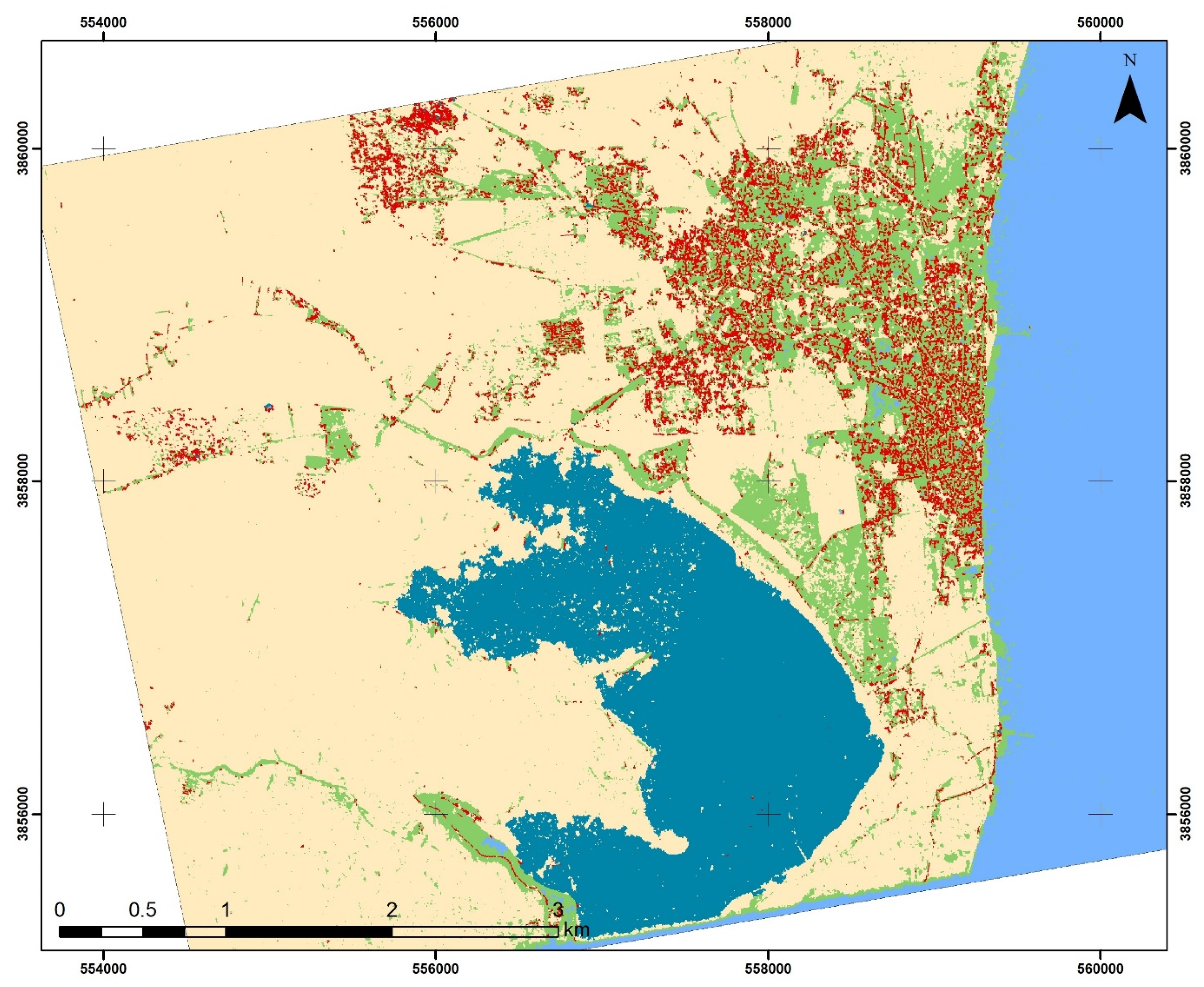
The outcomes of the classification process can be found in Figure 5. The different colours represent the different thematic classes selected before. Urban and other build-up areas are shown with red and land is shown with a yellow. Water bodies are light blue, while the salt lake is shown with dark blue. Finally, the vegetation is depicted with a green colour.
A closer look at the classification results of Figure 5 is shown in the following figure (Figure 6). Three examples are provided in this figure: (1) over the built-up areas of Larnaca city (first row, Figure 6), (2) near the Salt Lake of Larnaca (second row, Figure 6), and (3) an example of agricultural fields in the western part of the figure (third row, Figure 6).
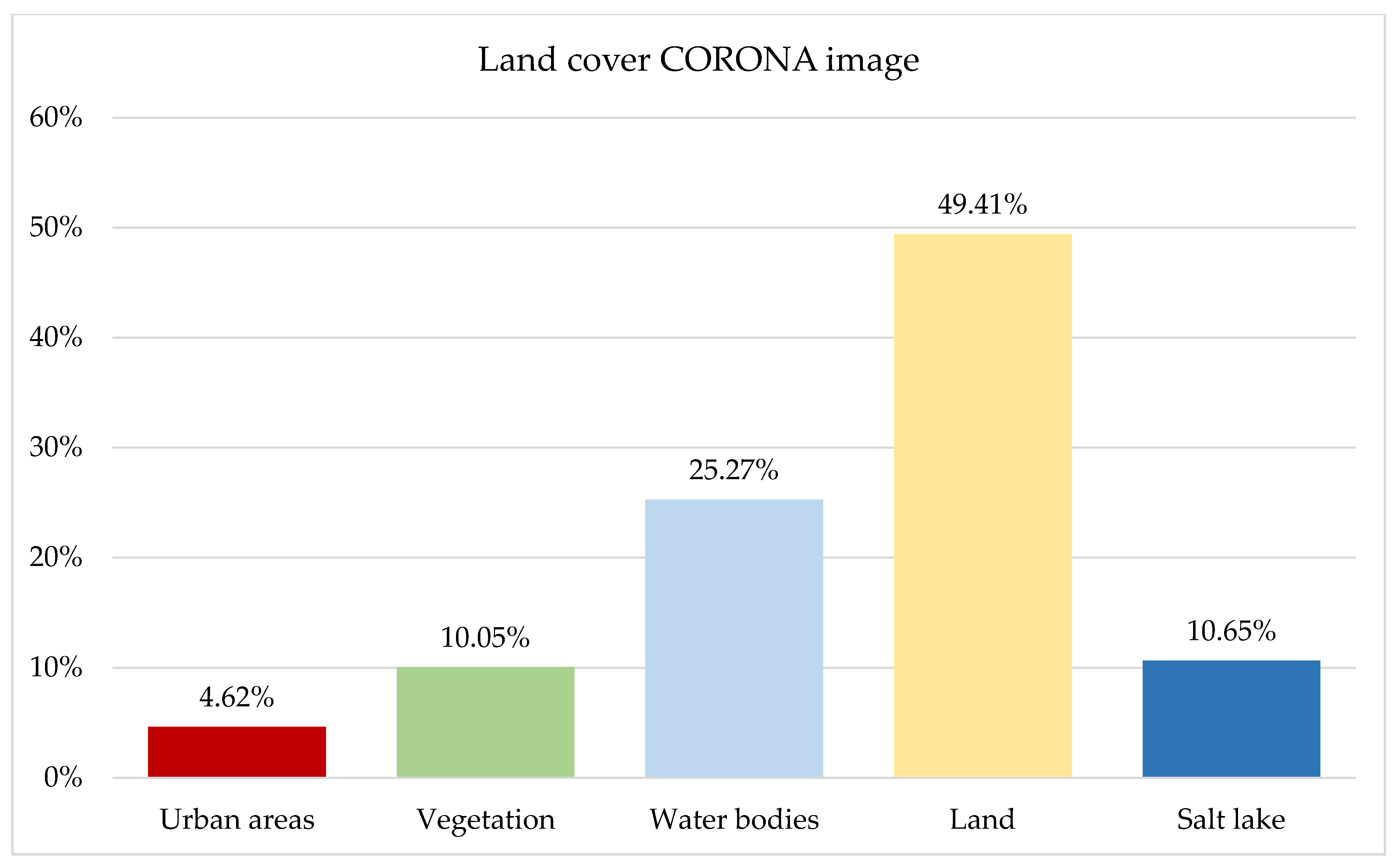
The land coverage of each class, in percentage, is shown in Figure 7. As is indicated, the class "land" covers approximately half of the image area (49.41%), while a significant proportion of the image is characterised as “water bodies” (25.27%). The “vegetation” and the “salt lake” are estimated to be at 10.05% and 10.65%, respectively. Finally, the urban areas are only a small part of the image, less than 5% (4.62%).
An error matrix has been tabulated to evaluate the classification results, and from there, other statistics have been generated. Based on the error matrix, we can estimate the overall accuracy of classification outcome and the accuracy per class. In this study, we have used 250 random points scattered all over the image. The class for each one of these points was then generated automatically from the GIS environment, while the correct (true) class was visually interpreted and recorded. Therefore, for each class, both the classification outcome and the true class were retrieved. The overall results of this analysis are shown in Table 2.
The overall accuracy was calculated at 0.94, while the kappa coefficient was estimated to be 0.91. The accuracy per thematic class was estimated as follows: for urban areas = 89%, for vegetation = 80%, for water bodies = 96%, for land = 97%, and for salt lakes = 81%.
It is therefore evident from the classification statistics that high accuracy can be achieved for producing historical land cover maps (>90%); however, the accuracy for each class can vary (from 81% to 97%). Nevertheless, these numbers remain high (close or higher than 85%), which are considered reasonable by the literature for developing thematic land cover maps (see, for instance, CORINE classification thematic accuracy, [14]).
4. Discussion
The overall methodology presented in this study is composed of two main steps: the colourisation of the CORONA image using deep learning modelling and the image classification using segmentation and a machine learning classifier. The latter has been achieved with high accuracy; however, variations between the classes were reported. Indeed, we can report a good correspondence between the land cover classification results and the original CORONA image, as shown in Figure 6. The first column of Figure 6 shows the CORONA image, the second column in Figure 6 shows the colourised image, and the third image displays the classification result.
The accuracy of the classification result obtained is similarly and sometimes improved compared to other relevant studies that have used different classification strategies. For instance, in [45], the Kappa coefficient was estimated to be between 0.81 and 0.90, while in [46], the accuracy was estimated to be between 0.60 and 0.88. In these examples and elsewhere, the classification of the CORONA image was performed using input multiband images from the original CORONA image (e.g., through texture analysis). In contrast, in this study, we propose colourised CORONA input layers (red-green-blue).
Of course, this approach has its shortcomings. Three false positive classification results have been observed through this process. The first one regards the classification of the shallow waters as vegetation instead of water bodies. Despite the efforts made to improve these results through the additional training sampling, the problem remained, as this is evident in the first row of Figure 6 (last column). The presence of the near-infrared spectral band could improve the outcome results due to the characteristic of water bodies to absorb the electromagnetic radiation in this part of the spectrum (approximately between 760–900 nm).
The second problem that occurred through the classification process regarded the incorrect classification of the land area as urban. This was visible in areas where we had a bright tone of soil, similar to the spectral profile of the urban areas. The use of texture analysis is expected to improve this mismatch. Finally, another mismatch was observed regarding the classification of the salt lake and especially in its boundaries, as this was classified as land.
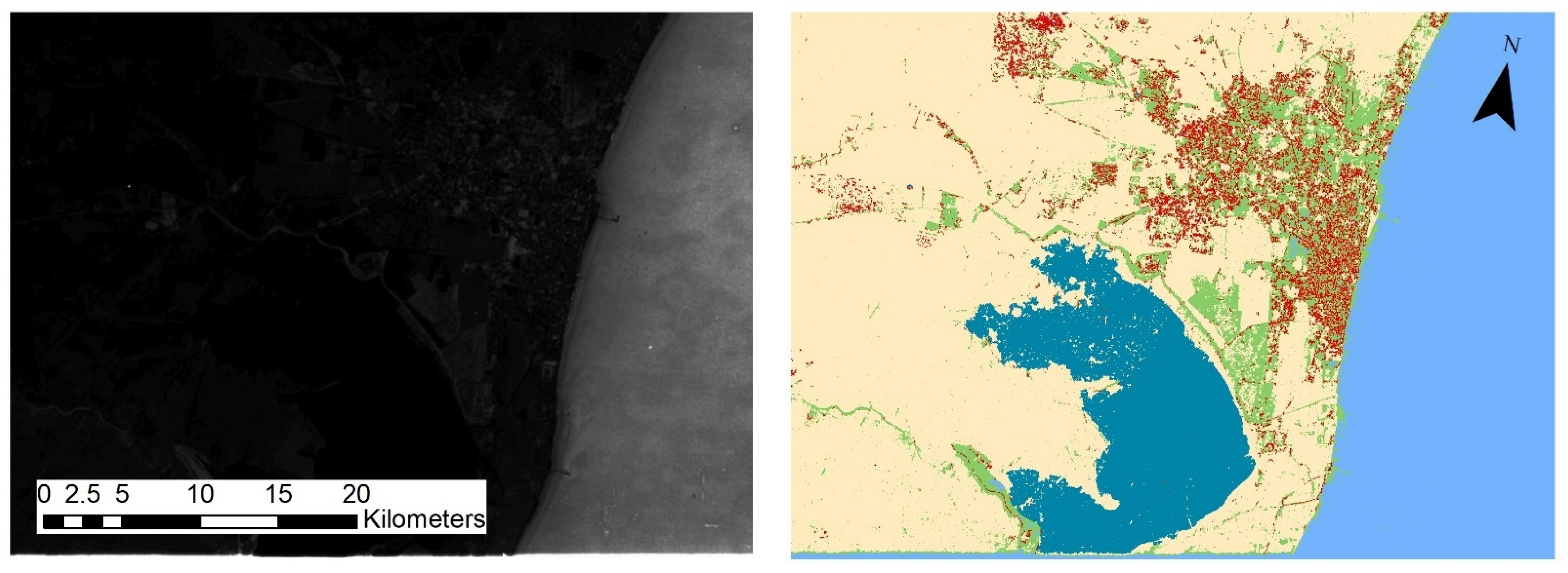
A major concern that remains, beyond the classification accuracy, is the colourisation process. As mentioned earlier (see quality metrics), the colourised image used for the classification process is not the same as the original greyscale CORONA image. An example from the results from the image quality metrics is visualised in Figure 8. On the left part of Figure 8, we can see the results of the ERGAS metric. Areas that have not changed between the colourisation process are visualised with a dark tone of grey, while areas that have changed through the colourisation process are shown with brighter grey tones. As shown, most of the changes are primarily observed in the water bodies on the eastern part of the image. Minor changes are also observed in other parts of the image, like near the salt lake and within the urban area (Larnaca city). This metric image can be used as an index of truthfulness for the classification results (see Figure 8 on the right part), going a step above and beyond the traditional classification accuracy. This index can also be helpful to explain some errors in the classification outcomes.
5. Conclusions
Historical land cover maps are important for several applications spanning from environmental studies to historical analysis. In addition, these maps can be beneficial to better understand the changes in the landscape, especially in areas where significant urbanisation has been reported in recent decades.
Although traditional classification techniques and other more sophisticated methods can produce high accuracy landcover maps, these can be generated through high-resolution multispectral satellite data. In contrast, historical archive satellite data does not have the same resolution, neither spectral nor spatial, which makes the process of classification difficult.
This study used the CORONA image, a widely known archive satellite dataset available only in recent years. The spectral resolution from the specific sensor was limited to the panchromatic spectral band, thus providing only greyscale images. For this reason, the classification process cannot be performed in a traditional multispectral dimensional space. Several attempts have been made in the literature to solve this problem, mainly by adding additional layers of information through texture information. Other studies have attempted to perform supervised classification and evaluate the overall results.
This study proposed an alternative method where the greyscale image is firstly colourised using pre-defined deep learning models. Then, an OBIA classification process is applied through the segmentation and the application of machine learning classifiers. The outcomes can be evaluated in both steps. Quality metrics can be applied to compare the original image against the colourised product. Then, a confusion matrix and a classification accuracy can be estimated for the land cover product.
The overall results were found to be promising, providing a land cover map with high accuracy: more than 85% overall accuracy and a kappa coefficient of 0.91. The proposed methodology can be implemented in any other greyscale image, whether they were taken from space or air. Future improvements can be made towards the automation of the classification process based on spectral libraries of specific thematic classes and integrating other input multiband images (e.g., after texture processing) to improve the results further. The ultimate goal is to develop a pre-defined deep learning model for colourisation purposes using training samples from CORONA and other historical satellite data.
Funding
This paper was submitted under the NAVIGATOR project. This work was co-funded by the European Regional Development Fund and the Republic of Cyprus through the Research and Innovation Foundation (Project: EXCELLENCE/0918/0052, Copernicus Earth Observation Big Data for Cultural Heritage).
Acknowledgments
The author would like to thank MyHeritage for providing access to the deep learning colourisation model and the access for the “heritage in colour” tool. The author would like to thank all reviewers for their valuable comments for improvements to the article. The CORONA image used in this study is openly available from the Earth Resources Observation and Science (EROS) Center of the United States Geological Survey (USGS). The quality metrics code used for the evaluation of the colourised image can be found in [40].
Conflicts of Interest
The author declares no conflict of interest.
References
- Regasa, M.S.; Nones, M.; Adeba, D. A Review on Land Use and Land Cover Change in Ethiopian Basins. Land 2021, 10, 585. [Google Scholar] [CrossRef]
- Chang, Y.; Hou, K.; Li, X.; Zhang, Y.; Chen, P. Review of Land Use and Land Cover Change research progress. IOP Conf. Series Earth Environ. Sci. 2018, 113, 012087. [Google Scholar] [CrossRef]
- Kuang, W.; Du, G.; Lu, D.; Dou, Y.; Li, X.; Zhang, S.; Chi, W.; Dong, J.; Chen, G.; Yin, Z.; et al. Global observation of urban expansion and land-cover dynamics using satellite big-data. Sci. Bull. 2021, 66, 297–300. [Google Scholar] [CrossRef]
- Alemayehu, F.; Tolera, M.; Tesfaye, G. Land use land cover change trend and its drivers in Somodo watershed south western, Ethiopia. Afr. J. Agric. Res. 2019, 14, 102–117. [Google Scholar]
- Hou, J.; Qin, T.; Liu, S.; Wang, J.; Dong, B.; Yan, S.; Nie, H. Analysis and Prediction of Ecosystem Service Values Based on Land Use/Cover Change in the Yiluo River Basin. Sustainability 2021, 13, 6432. [Google Scholar] [CrossRef]
- Delia, K.A.; Haney, C.R.; Dyer, J.L.; Paul, V.G. Spatial Analysis of a Chesapeake Bay Sub-Watershed: How Land Use and Precipitation Patterns Impact Water Quality in the James River. Water 2021, 13, 1592. [Google Scholar] [CrossRef]
- Amoakoh, A.O.; Aplin, P.; Awuah, K.T.; Delgado-Fernandez, I.; Moses, C.; Alonso, C.P.; Kankam, S.; Mensah, J.C. Testing the Contribution of Multi-Source Remote Sensing Features for Random Forest Classification of the Greater Amanzule Tropical Peatland. Sensors 2021, 21, 3399. [Google Scholar] [CrossRef] [PubMed]
- Paluba, D.; Laštovička, J.; Mouratidis, A.; Štych, P. Land Cover-Specific Local Incidence Angle Correction: A Method for Time-Series Analysis of Forest Ecosystems. Remote Sens. 2021, 13, 1743. [Google Scholar] [CrossRef]
- Ghayour, L.; Neshat, A.; Paryani, S.; Shahabi, H.; Shirzadi, A.; Chen, W.; Al-Ansari, N.; Geertsema, M.; Pourmehdi Amiri, M.; Gholamnia, M.; et al. Performance Evaluation of Sentinel-2 and Landsat 8 OLI Data for Land Cover/Use Classification Using a Comparison between Machine Learning Algorithms. Remote Sens. 2021, 13, 1349. [Google Scholar] [CrossRef]
- Guo, L.; Xi, X.; Yang, W.; Liang, L. Monitoring Land Use/Cover Change Using Remotely Sensed Data in Guangzhou of China. Sustainability 2021, 13, 2944. [Google Scholar] [CrossRef]
- Șerban, R.-D.; Șerban, M.; He, R.; Jin, H.; Li, Y.; Li, X.; Wang, X.; Li, G. 46-Year (1973–2019) Permafrost Landscape Changes in the Hola Basin, Northeast China Using Machine Learning and Object-Oriented Classification. Remote Sens. 2021, 13, 1910. [Google Scholar] [CrossRef]
- Hussain, M.; Chen, D.; Cheng, A.; Wei, H.; Stanley, D. Change detection from remotely sensed images: From pixel-based to object-based approaches. ISPRS J. Photogramm. Remote Sens. 2013, 80, 91–106. [Google Scholar] [CrossRef]
- Myint, S.W.; Gober, P.; Brazel, A.; Grossman-Clarke, S.; Weng, Q. Per-pixel vs. object-based classification of urban land cover extraction using high spatial resolution imagery. Remote Sens. Environ. 2011, 115, 1145–1161. [Google Scholar] [CrossRef]
- Ullah, S.; Tahir, A.A.; Akbar, T.A.; Hassan, Q.K.; Dewan, A.; Khan, A.J.; Khan, M. Remote Sensing-Based Quantification of the Relationships between Land Use Land Cover Changes and Surface Temperature over the Lower Himalayan Region. Sustainability 2019, 11, 5492. [Google Scholar] [CrossRef] [Green Version]
- Hishe, H.; Giday, K.; Van Orshoven, J.; Muys, B.; Taheri, F.; Azadi, H.; Feng, L.; Zamani, O.; Mirzaei, M.; Witlox, F. Analysis of Land Use Land Cover Dynamics and Driving Factors in Desa’a Forest in Northern Ethiopia. Land Use Policy 2021, 101, 105039. [Google Scholar] [CrossRef]
- Hong, C.; Burney, J.A.; Pongratz, J.; Nabel, J.E.; Mueller, N.D.; Jackson, R.B.; Davis, S.J. Global and regional drivers of land-use emissions in 1961–2017. Nat. Cell Biol. 2021, 589, 554–561. [Google Scholar] [CrossRef]
- Huang, X.; Huang, J.; Wen, D.; Li, J. An updated MODIS global urban extent product (MGUP) from 2001 to 2018 based on an automated mapping approach. Int. J. Appl. Earth Obs. Geoinform. 2021, 95, 102255. [Google Scholar] [CrossRef]
- Gong, P.; Li, X.; Wang, J.; Bai, Y.; Chen, B.; Hu, T.; Liu, X.; Xu, B.; Yang, J.; Zhang, W.; et al. Annual maps of global artificial impervious area (GAIA) between 1985 and 2018. Remote Sens. Environ. 2020, 236, 111510. [Google Scholar] [CrossRef]
- Tariq, A.; Shu, H.; Kuriqi, A.; Siddiqui, S.; Gagnon, A.S.; Lu, L.; Linh, N.T.; Pham, Q.B. Characterization of the 2014 Indus River Flood Using Hydraulic Simulations and Satellite Images. Remote Sens. 2021, 13, 2053. [Google Scholar] [CrossRef]
- Alexakis, D.D.; Hadjimitsis, G.D.; Agapiou, A. Integrated use of remote sensing, GIS and precipitation data for the assessment of soil erosion rate in the catchment area of “Yialias” in Cyprus. Atmos. Res. 2013, 131, 108–124. [Google Scholar] [CrossRef]
- Alewell, C.; Borrelli, P.; Meusburger, K.; Panagos, P. Using the USLE: Chances, challenges and limitations of soil erosion modelling. Int. Soil Water Conserv. Res. 2019, 7, 203–225. [Google Scholar] [CrossRef]
- CORINE Land Cover. Available online: https://land.copernicus.eu/pan-european/corine-land-cover (accessed on 6 July 2021).
- Copernicus Land Monitoring Service, CORINE Land Cover. Available online: https://land.copernicus.eu/user-corner/technical-library/clc-product-user-manual (accessed on 6 July 2021).
- USGS EROS Archive—Declassified Data—Declassified Satellite Imagery—1. Available online: https://www.usgs.gov/centers/eros/science/usgs-eros-archive-declassified-data-declassified-satellite-imagery-1?qt-science_center_objects=0#qt-science_center_objects (accessed on 6 July 2021).
- Ulloa-Torrealba, Y.; Stahlmann, R.; Wegmann, M.; Koellner, T. Over 150 Years of Change: Object-Oriented Analysis of Historical Land Cover in the Main River Catchment, Bavaria/Germany. Remote Sens. 2020, 12, 4048. [Google Scholar] [CrossRef]
- Liu, D.; Toman, E.; Fuller, Z.; Chen, G.; Londo, A.; Zhang, X.; Zhao, K. Integration of historical map and aerial imagery to characterise long-term land-use change and landscape dynamics: An object-based analysis via Random Forests. Ecol. Indic. 2018, 95, 595–605. [Google Scholar] [CrossRef]
- Gobbi, S.; Ciolli, M.; La Porta, N.; Rocchini, D.; Tattoni, C.; Zatelli, P. New Tools for the Classification and Filtering of Historical Maps. Int. J. Geo-Inf. 2019, 8, 455. [Google Scholar] [CrossRef] [Green Version]
- Talich, M. Classification of digitised old maps and possibilities of its utilisation. ePerimetron 2012, 7, 11. [Google Scholar]
- Jabs-Sobocińska, Z.; Affek, A.N.; Ewiak, I.; Nita, M.D. Mapping Mature Post-Agricultural Forests in the Polish Eastern Carpathians with Archival Remote Sensing Data. Remote Sens. 2021, 13, 2018. [Google Scholar] [CrossRef]
- Shahtahmassebi, A.R.; Lin, Y.; Lin, L.; Atkinson, P.M.; Moore, N.; Wang, K.; He, S.; Huang, L.; Wu, J.; Shen, Z.; et al. Reconstructing Historical Land Cover Type and Complexity by Synergistic Use of Landsat Multispectral Scanner and CORONA. Remote Sens. 2017, 9, 682. [Google Scholar] [CrossRef] [Green Version]
- Li, L.X.; Lambin, E.F.; Wu, W.; Servais, M. Land-cover changes in tarim basin (1964–2000): Application of post-classification change detection technique. In Ecosystems Dynamics, Ecosystem-Society Interactions, and Remote Sensing Applications for Semi-Arid and Arid Land; Pan, X., Gao, W., Glantz, M.H., Honda, Y., Eds.; SPIE: Bellingham, CD, USA, 2003. [Google Scholar]
- Cetin, M. A satellite based assessment of the impact of urban expansion around a lagoon. Int. J. Environ. Sci. Technol. 2009, 6, 579–590. [Google Scholar] [CrossRef] [Green Version]
- Andersen, G.L. How to detect desert trees using corona images: Discovering historical ecological data. J. Arid. Environ. 2006, 65, 491–511. [Google Scholar] [CrossRef] [Green Version]
- Deshpande, P.; Belwalkar, A.; Dikshit, O.; Tripathi, S. Historical land cover classification from CORONA imagery using convolutional neural networks and geometric moments. Int. J. Remote Sens. 2021, 42, 5144–5171. [Google Scholar] [CrossRef]
- Agapiou, A.; Alexakis, D.D.; Sarris, A.; Hadjimitsis, D.G. Colour to Greyscale Pixels: Re-seeing Greyscale Archived Aerial Photographs and Declassified Satellite CORONA Images Based on Image Fusion Techniques. Archaeol. Prospect. 2016, 23, 231–241. [Google Scholar] [CrossRef]
- USGS. Earth Explorer Service. Available online: https://earthexplorer.usgs.gov/ (accessed on 2 April 2021).
- MyHeritage in ColorTM. Available online: https://www.myheritage.com/incolor (accessed on 8 June 2021).
- DeOldify Deep Learning Model. Available online: https://github.com/jantic/DeOldify/blob/master/README.md (accessed on 8 July 2021).
- Ghassemian, H. A review of remote sensing image fusion methods. Inf. Fusion 2016, 32, 75–89. [Google Scholar] [CrossRef]
- Vaiopoulos, A.D. Developing Matlab scripts for image analysis and quality assessment. In Proc. SPIE 8181, Earth Resources and Environmental Remote Sensing/GIS Applications II; International Society for Optics and Photonics: Bellingham, WA, USA, 2011; p. 81810B. [Google Scholar]
- Wang, Z.; Brenning, A. Active-Learning Approaches for Landslide Mapping Using Support Vector Machines. Remote Sens. 2021, 13, 2588. [Google Scholar] [CrossRef]
- Chang, C.-C.; Lin, C.-J. LIBSVM: A Library for Support Vector Machines. ACM Trans. Intell. Syst. Technol. 2011, 2, 27. Available online: http://www.csie.ntu.edu.tw/~cjlin/libsvm (accessed on 18 July 2021). [CrossRef]
- Hsu, C.-W.; Chang, C.-C.; Lin, C.-J. A Practical Guide to Support Vector Classification; National Taiwan University: Taipei, Taiwan, 2010; Available online: http://www.csie.ntu.edu.tw/~cjlin/papers/guide/guide.pdf (accessed on 18 July 2021).
- Wu, T.-F.; Lin, C.-J.; Weng, R.C. Probability Estimates for Multi-Class Classification by Pairwise Coupling. J. Mach. Learn. Res. 2004, 5, 975–1005. Available online: http://www.csie.ntu.edu.tw/~cjlin/papers/svmprob/svmprob.pdf (accessed on 18 July 2021).
- Song, D.-X.; Huang, C.; Sexton, J.O.; Channan, S.; Feng, M.; Townshend, J.R. Use of Landsat and Corona data for mapping forest cover change from the mid-1960s to 2000s: Case studies from the Eastern United States and Central Brazil. ISPRS J. Photogramm. Remote Sens. 2015, 103, 81–92. [Google Scholar] [CrossRef] [Green Version]
- Saleem, A.; Corner, R.; Awange, J. On the possibility of using CORONA and Landsat data for evaluating and mapping long-term LULC: Case study of Iraqi Kurdistan. Appl. Geogr. 2018, 90, 145–154. [Google Scholar] [CrossRef]
Figure 1.
Methodology of the study.

Figure 2.
CORONA greyscale satellite image over Larnaca city (1963).

Figure 3.
CORONA colourised satellite image over Larnaca city (1963).

Figure 4.
A closer look at the colourised CORONA satellite image over Larnaca city (a), the surrounding agricultural area (b) and over the salt lake of Larnaca (c). The left column shows the original greyscale CORONA image, while the right column shows the colourised image.
Figure 4.
A closer look at the colourised CORONA satellite image over Larnaca city (a), the surrounding agricultural area (b) and over the salt lake of Larnaca (c). The left column shows the original greyscale CORONA image, while the right column shows the colourised image.

Figure 5.
Classification results of the colourised CORONA image. The land is shown with a yellow colour, water with light blue, the salt lake with dark blue colour, vegetation with green colour, and urban areas with red colour.
Figure 5.
Classification results of the colourised CORONA image. The land is shown with a yellow colour, water with light blue, the salt lake with dark blue colour, vegetation with green colour, and urban areas with red colour.

Figure 6.
A closer look over the classification results as indicated in Figure 5. The first row displays the results over Larnaca urban area. The second row shows the results over the Salt Lake of Larnaca. Finally, the third row shows an example from the agricultural fields in the western part of the image. The first column shows the results of the original CORONA image, the second column the colourised CORONA image and the third colour the classification outcomes with the different thematic classes. The colours are the same as in Figure 5.

Figure 7.
Land cover proportions (%) for the five main classes of the classification analysis.

Figure 8.
(Left): Image quality metric (ERGAS) comparing the original CORONA image against the colourised CORONA image. Similarities between the two images are shown with a dark tone, while areas that have changed through the colourisation process are white. (Right): the classification outcome of the colourised CORONA image.


Table 1.
Quality metrics results.
| Quality Metric | Equation | Result |
|---|---|---|
| Bias | (1) | 0.236 |
| image entropy | (2) | 0.249 |
| ERGAS | (3) | 5.256 |
| RASE | (4) | 25.015 |
| RMSE | (5) | 12.932 |
Table 2.
Error matrix of the classification outcomes. The diagonal results, indicated as bold, represent the number of points for which the predicted label is equal to the true label, while off-diagonal results are those that are mislabeled by the classifier.
Table 2.
Error matrix of the classification outcomes. The diagonal results, indicated as bold, represent the number of points for which the predicted label is equal to the true label, while off-diagonal results are those that are mislabeled by the classifier.
| Reference | Total | ||||||
|---|---|---|---|---|---|---|---|
| Class | U | V | W | L | SL | ||
| Classification | U | 8 | 0 | 0 | 0 | 0 | 8 |
| V | 0 | 16 | 2 | 0 | 0 | 18 | |
| W | 0 | 2 | 69 | 1 | 0 | 72 | |
| L | 1 | 2 | 0 | 122 | 5 | 130 | |
| SL | 0 | 0 | 0 | 1 | 21 | 22 | |
| Total | 9 | 20 | 71 | 124 | 26 | 250 | |
Publisher’s Note: MDPI stays neutral with regard to jurisdictional claims in published maps and institutional affiliations. |
© 2021 by the author. Licensee MDPI, Basel, Switzerland. This article is an open access article distributed under the terms and conditions of the Creative Commons Attribution (CC BY) license (https://creativecommons.org/licenses/by/4.0/).
Share and Cite
MDPI and ACS Style
Agapiou, A. Land Cover Mapping from Colorized CORONA Archived Greyscale Satellite Data and Feature Extraction Classification. Land 2021, 10, 771. https://0-doi-org.brum.beds.ac.uk/10.3390/land10080771
AMA Style
Agapiou A. Land Cover Mapping from Colorized CORONA Archived Greyscale Satellite Data and Feature Extraction Classification. Land. 2021; 10(8):771. https://0-doi-org.brum.beds.ac.uk/10.3390/land10080771
Chicago/Turabian StyleAgapiou, Athos. 2021. "Land Cover Mapping from Colorized CORONA Archived Greyscale Satellite Data and Feature Extraction Classification" Land 10, no. 8: 771. https://0-doi-org.brum.beds.ac.uk/10.3390/land10080771
Note that from the first issue of 2016, this journal uses article numbers instead of page numbers. See further details here.