New Round of Collective Forest Rights Reform, Forestland Transfer and Household Production Efficiency

Abstract

The purpose of this paper was to analyze the influence mechanism of the new round of Collective Forest Rights Reform (CFRR) on farmers’ production efficiency from the perspective of forestland transfer. Based on the panel data of field investigation in Jiangxi Province, a panel logit model was used to verify whether the new round of CFRR has affected farmers’ forestland circulation behavior. The results showed that the new round of CFRR has played a significant role in promoting forestland circulation. Secondly, the non-parametric DEA method was used to estimate the technical, scale, and comprehensive efficiency of households. DID and panel quantile models were constructed to analyze the impact of forestland inflow policy and forestland outflow policy effects on rural household productivity. The regression results showed that the effect of forestland inflow has had a significantly positive impact on scale and comprehensive efficiency, but it only had a significant effect on technical efficiency in the 0.1 quartile. The effect of forestland outflow was not found to be significant for technical, scale, and comprehensive efficiency, but it was found to be negative for technical efficiency in the 0.75 quartile and negative for scale efficiency in the 0.5 and 0.75 quantiles.

1. Introduction

China is a large agricultural country. By the end of 2020, China’s rural population was 510 million. Though it showed a downward trend, it still accounted for 36.11% of the total population [1]. The level of farmers’ production efficiency has a significant impact on the improvement of China’s productivity. Since China’s reform in 1978, improving farmers’ production efficiency has been the focus of policy makers [2]. The implementation of the Household Contract Responsibility System (HCRS) for agricultural land has achieved great success and is considered to be an effective policy for improving the production efficiency of farmers [3]. Consequently, following the example of agricultural land, China began to carry out a series of reforms on woodlands in order to improve the production efficiency of farmers by reforming their forestry practice.

Understanding patterns of change across land property is essential for policies that foster healthy and resilient forests for the future [4]. Using data from surveys of African American forest landowners in Georgia, Goyke and other scholars used the Theory of Planned Behavior to offer a framework for understanding the role of ownership structures, along with other landowner characteristics on forest management intentions and behaviors; the results showed that the ownership structures have no statistically significant effect on goal setting or forest management activity [5]. Improving production efficiency lies in the effective use of farmers’ input of production factors. However, the development of China’s factor market has not been perfect (the development of the land factor market, especially, lags behind), which has greatly hindered the improvement of farmers’ production efficiency. In order to promote the development of the forest land factor market, the new round of CFRR in China in 2003 rearranged forest land property rights, e.g., giving farmers the right to the use of forest land, the right of disposal, the right of income, and the implementation of relevant supporting measures (see Section 3.1 for details). These measures were intended to improve the security of farmers’ property rights in order to establish a standardized forestland transfermarket and promote farmers’ forestland transfer behavior [6,7,8]. Though many scholars have theoretically analyzed the positive promotion effect of collective forest right reform on forestland transfer [9,10,11,12], there has been little empirical evidence in the literature.

Land property has been used to understand the long-term effects of and variation in land management [4]. Using a case study of Liaoning province, China, and using forestland plots as the decision-making unit, Lu et al. [13] analyzed the influencing factors of forestland production efficiency through econometric analysis. Their results showed that rural households’ willingness to transfer forestland is weak and the frequency of forestland transfer is relatively low; without action, forestland transfers can be expected to continue to fail to fulfil their potential in stimulating production efficiency.

In recent years, the efficiency of forestland production has gradually become an important field of inquiry for the academic community, both at home and abroad [14]. Many scholars have studied the relationship between land transfer and farmers’ production efficiency. The empirical analyses of different scholars based on the survey data of different provinces in China have revealed that the forestland transfer behavior generally improves the production efficiency of farmers [15,16]. Based on the data of Beijing, Shanghai, Guangzhou, and other places, Chen et al. [17] concluded that land transfer reduces the technical efficiency and improves the scale efficiency of farmers. Many scholars have subdivided land transfer into land inflow and outflow behavior, and they have found that land inflow and land outflow have different effects on farmers’ production efficiency; it is controversial whether land outflow has a significant impact on farmers’ productivity. On the one hand, the empirical results of different scholars have shown that the inflow of land has a positive impact on the productivity of farmers. The usual explanation is that the development of the land market makes the land flow to more efficient farmers. On the other hand, the empirical results of some scholars have shown that land outflow has a significantly positive impact on farmers’ production efficiency, although this impact is lower than that of land inflow [18]. However, other scholars have found that land outflow has no effect on farmers’ productivity [14,19]. These conflicting results may be due to the use of different research data and the fact that the impact of land outflow on farmers’ productivity is different in different areas.

At present, the calculation of farmers’ production efficiency is generally based on the level of forestland (agricultural land), i.e., only the farmers’ forestry (agricultural) production decisions are considered, which are independent of non-agricultural production and management. The irrationality of this calculation method lies in its ignorance of the incompleteness of China’s agricultural factor markets and the interdependence between the production function corresponding to agricultural (forestry) production and non-agricultural production function. Therefore, following the work of Chavas et al. [20], this paper was based on the rural household level, i.e., we considered the agricultural operation and non-agricultural employment behavior of farmers at the same time to estimate the production efficiency of farmers.

The purpose of this study was twofold. We intended to first verify the promotion effect of the new round of CFRR on farmers’ forestland transfer behavior and second analyze the impact of different forest land transfer behaviors (inflow and outflow) on farmers’ production efficiency. Accordingly, the contributions of this study are as follows. Though there have been many studies on the relationship between land transfer and farmers’ production efficiency, there have been few studies on forest land, a gap that this paper is intended to fill. Second, for this paper, farmers’ agricultural production and management and non-agricultural production and management behaviors were considered at the same time to more reasonably predict farmers’ production efficiency, which corrects the commonly used but inaccurate estimations methods of production efficiency. Third, the influence of forestland inflow and outflow on farmers with different production efficiency levels was analyzed.

The following sections of this paper are arranged as follows. The Section 2 is a review of the history of China’s CFRR. The Section 3 presents a theoretical investigation of the relationship among the new round of CFRR, forest land transfer behavior, and farmers’ production efficiency. The Section 4 introduces the model of the empirical test. The Section 5 reports the results and discussion of the empirical test. The Section 6 is a summary.

2. The Background of CFRR

With the success of the HCRS’s reforms of agricultural land, people began to pay more attention to the forestry sector’s production potential. Forest land in China is owned by the state and collectives, and the reforms have mainly been aimed at some forest land owned by collectives. To date, the reform of collective forest rights has gone through three stages: (1) the “three fixed” reform stage from 1978 to 1992, (2) the pilot stage of forest right reform from 1993 to 2003, and (3) a new round of CFRR in 2003. The redistribution of forest land property rights has remained throughout reform stages [21]. Forest land property rights comprise a series of right bundles, including forest land ownership, use right, income rights, and disposition rights [22].

2.1. The “Three Fixed” Reform Stage from 1978 to 1992

The “three fixed” reform was a long-term and far-reaching reform that was implemented at the county level in 1981. By 1986, farmers had contracted nearly 70% of collectively-owned forest land [23]. In this reform, the property rights of forest land were divided into three types: self-retained mountain, responsible mountain, and collectively-owned forest land. Compared with collectively-owned forest land, farmers on self-retained mountain land had the right to manage forest land and own the trees planted on the land. The responsible mountain type was different from the self-retained mountain type in that the collective owned the ownership of the forest land and trees, so management decisions are jointly made by the collective and contractor. Collectively owned forest land management and ownership rights were possessed by collectives, and their real executors were the leaders of village collectives.

Though restrictions were relaxed and partial private ownership was allowed during the “three fixed” reform period, there were still some problems. For instance, scattered farmers lacked funds for fire prevention, mountains were divided according to population, the boundaries and ownership of forest land were unclear, the phenomenon of deforestation was serious, and village cadres engaged in the unreasonable management of collective forest land harvesting income and expenditure. Most importantly, during the “three fixed” reform period, because the management rights and ownership of forest land were possessed by collectives, the circulation of forest land was not legally allowed, forest land transfer occurred less, and farmers’ ability to privately circulate forest land could not be protected.

2.2. The Pilot Stage of Forest Right Reform from 1993 to 2003

In the ten years following the “three fixed” reform, attempts were made to solve its problems. First of all, forest land was placed under collective ownership, while forest land use rights and forest ownership were given to farmers. Secondly, the income and disposition rights of forest land were distributed between farmers and collectives, the collectives collected rent from farmers, and farmers were provided residual income rights.

Under this reform, there were huge problems in forest land transfer. Though the revised Forest Law in 1998 explicitly allowed for the behavior of forest land transfer in law, the absence of standardized and sound forest land transfer policy, forest land transfer contract, and forest land evaluation systems led to the large-scale households contracting forest land, low transfer prices, and rent-seeking behavior of collective leaders.

2.3. A New Round of CFRR in 2003

In 2003, a new round of CFRR started in Fujian Province was supported by the central government and quickly spread to other provinces in Southern China. China began to comprehensively promote the CFRR reform in 2008 to clarify contract and management rights, giving households the right to transfer forestland, become shareholders in forestry enterprises, and mortgage forest land to obtain forestry loans [24]. In 2008, “Opinions of CPC Central Committee and State Council on Comprehensively Promoting the Reform of Collective Forest Right” designated households as the main body of forestry management. The new round of CFRR was characterized by the redistribution of the right to use collective forest land, including issuing forest right certificates to farmers to determine their right to use, the duration of the right to use, and the boundaries of forest land. In the above mentioned government document, it is clear that the duration of the right to use forest land was 70 years, allowing forest land to be mortgaged and farmers to enjoy the right to obtain income from forest land. It is noteworthy that this reform encouraged farmers’ forest land transfer behavior. In addition to the abovementioned confirmation and certification, farmers were given more complete forest land property rights, and supporting measures such as creating a forest land transfer center and a forest land evaluation system, were also introduced to establish a standardized forest land transfer market. This reform was highly anticipated by policy makers and scholars, who hoped to arouse farmers’ enthusiasm for production and to improve their income and welfare levels.

3. Theoretical Analysis

3.1. Theoretical Analysis of the Promotion Effect of the New Round of CFRR on Farmers’ Forest Land Transfer Behavior

As recalled in the previous section, although the “three fixed” reform divided the self-retained and responsible mountains and farmers had the right to use forest land to a certain extent, China’s forest land management still faced problems such as unclear forest land boundaries and ownership, illegal logging, short forest land use and operation cycles, and heavy taxes and fees [25,26]. Before the new round of forest reform, farmers’ forest land property rights were incomplete and risked forest land adjustment, and farmers were faced with great insecurity of forest land property rights [27]. On the one hand, farmers’ forest land transfer behavior was restricted by policies and regulations; on the other hand, both sides were worried about the occurrence of forest land transfer disputes due to the lack of forest right certificates and the risk of forest land adjustments, which hindered the development and perfection of the forest land transfer market and thus limited the occurrence of forest land transfer behavior.

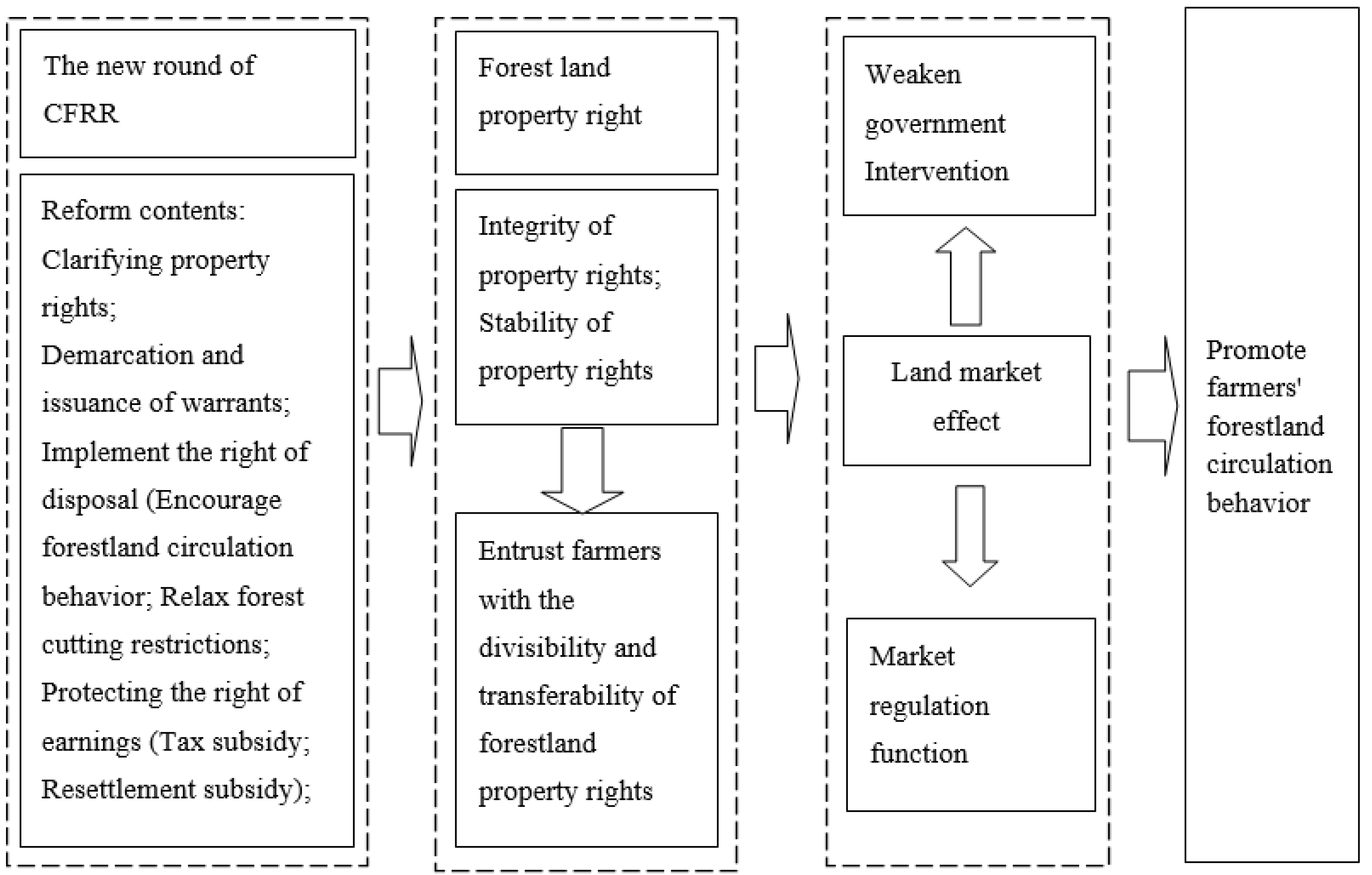
The 2003 CFRR was intended as a response to the dilemma of forestland management brought by the “three fixed” period. First, it clarified that farmers’ contract and management rights, forest ownership, and use rights were expanded to forest land, as well as that the contracting period of forest land was 70 years and can be renewed at the expiration of the contract. The government demarcated the farmers’ self-retained and responsible mountains, and they recorded these decisions in writing by issuing forest-warrants. In the 2008 “Opinions of CPC Central Committee and State Council on Comprehensively Promoting the Reform of Collective Forest Right”, it was clearly suggested to encourage farmers’ forest land transfer behavior, relax forest logging restrictions, allow farmers to use forest land for mortgage, reduce taxes, increase forestry subsidies, and establish forest land transfer platforms and forest assessment systems. Reform measures involved all aspects of forestland use rights, ownership, disposal, and income rights; improving the integrity and stability of farmers’ forestry rights; and increasing the security of farmers [28]. These reform measures have gradually made the government decrease the degree of the severability and transferability of farmers’ forest ownership, as well as make farmers directly face the market when they circulate forestland. At this time, farmers may make decisions regarding the leasing or selling land [6,29,30] based on changes in the external economic environment (especially the demand and supply of forest land changes) so that forest rights can be optimized and farmers’ families can achieve greater utility and benefits; this is the so-called land market effect. Following this analysis, the first research hypothesis of this paper can be put forward: collective forest rights reform can promote the farmers’ forest land transfer behaviors; details are shown in Figure 1.

3.2. Analysis on the Maximization of Profit at Household Level after the Occurrence of Farmers’ Forestland Transfer Behavior

Based on the research results of Chavas et al. [20], the authors of this paper built a housekeeping profit maximization model including the inflow behavior of farmers’ forest land. We assumed that the number of labors in a peasant household is $k$ and that these labors are allocated to forestry, agriculture, and off-farm employment activities by the household. The vector of labor time into forestry is $F_{for}=(F_{for1},F_{for2},F_{for3}\cdots F_{fork})$. where $F_{fori}$ represents the time spent by the $ith$ labor force in forestry production activities, $i=1,2,3\cdots k$. The rural household forestry output vector is $y_{for}$. Given the forestry market price vector $p_{for}$, the rural household forestry income is $p_{for}\ast y_{for}$. The labor time vector into agriculture is $F_{far}=(F_{far2},F_{far2},F_{far3}\cdots F_{fark})$. The agricultural output vector of rural households is $y_{far}$. Given the agricultural market price vector $p_{far}$, the agricultural income of rural households is $p_{far}\ast y_{far}$. The farmer’s initial forestland area is $L$. If the forestland flows in, the rent paid per mu (1 mu = 1/15 ha) is $R_{in}$. Assuming that the forestland flows into $L_{in}$ mu, the rent paid into the forestland is $R_{in}\ast L_{in}$; if the forestland flows out, the rent per mu is $R_{out}$. At the same time, farmers can hire labor $H$ at the market wage $w$. In addition, farmers are also engaged in non-agricultural employment. To simplify the model, the authors of this paper assumed that only labor is invested in non-agricultural business activities, the input time is $F_{non}=(F_{non2},F_{non2},F_{non3}\cdots F_{nonk})$, and non-farm employment income is $N$. Vector $X$ represents the input of other factors in the agricultural and forestry production process of farmers except for labor force and land, and its price is $p_x$. The technical constraints $T$ faced by farmers are $(X,F_{for},F_{far},H,F_{non},L,L_{in},L_{out};y_{far},y_{for},N)\in T$.

Suppose that the utility function of a rural household is $U(c,l)$, where c is the consumption of the rural household and l is the leisure of the household labor force; then, the utility function is a quasi-concave function of $(c,l)$. The utility maximization level is

$$\begin{array}{l}{\max }_{\begin{array}{l}X,F_{for},F_{far},\\ H,F_{non},L,L_{in},\\ L_{out};y_{far},y_{for},\\ N,R_{out},R_{in},c,l\end{array}}\left\{U(c,l):(X,F_{for},F_{far},H,F_{non},L,L_{in},L_{out};y_{far},y_{for},N)\in T\right\}\\ s.t.\hspace{1em}\hspace{1em}\hspace{1em}\hspace{1em}\{\begin{array}{c}{F}_{fari}+F_{fori}+F_{noni}=M-l,\begin{array}{cc}& \end{array}i=1,2,3\cdots k\\ c\le p_{for}\ast y_{for}+p_{far}\ast y_{far}-R_{in}\ast L_{in}+R_{out}\ast L_{out}-wH+N\end{array}\end{array}$$

(1)

where M represents the time owned by household labor. Formula (1) shows that the rural household labor force is constrained by working hours, and the rural household’s consumption ability is constrained by family income. The process of farmers realizing utility maximization comprises choosing the optimal consumption and leisure times $(c,l)$.

$$\begin{array}{l}{\max }_{c,l}\left\{U(c,l)\right\}\\ s.t.\begin{array}{cc}& c\le \pi \left(p_{for},p_{far},w,R_{in},R_{out},p_x,M-l\right)\end{array}\end{array}$$

(2)

Formula (2) indicates that the realization of utility maximization is based on the level of profit maximization.

The frontier of rural household production is determined by forestry income or output, agricultural income or output, the non-agricultural employment income of forest land transfer income and the input $X$ of agricultural means of production, and the total labor input of agricultural production and non-agricultural management $(M-l)$.

$$\begin{array}{l}\pi \left(p_{for},p_{far},w,R_{in},R_{out},p_x,M-l\right)\\ ={\max }_{\begin{array}{l}X,F_{for},F_{far},H,L,\\ F_{non};y_{far},y_{for},N,\\ R_{out},R_{in}\end{array}}\left\{\begin{array}{l}{p}_{for}\ast y_{for}+p_{far}\ast y_{far}-R_{in}\ast L_{in}\\ +R_{out}\ast L_{out}-wH-p_{x}X+N\end{array}\right\}\\ s.t.\begin{array}{cc}& F_{fari}+F_{fori}+F_{noni}=M-l,\begin{array}{c}\end{array}\end{array}i=1,2,3\cdots k\end{array}$$

(3)

Formula (3) shows that there is interdependence between agricultural production and non-agricultural production and management when farmers allocate resources. When farmers maximize their profits, the corresponding input variables can be expressed as $x^{*}\left(p_{for},p_{far},R_{in},R_{out},w,p_X,M-l\right)$, ${F_{for}}^{*}\left(p_{for},p_{far},R_{in},R_{out},w,p_X,M-l\right)$, ${F_{far}}^{*}\left(p_{for},p_{far},R_{in},R_{out},w,p_X,M-l\right)$, $H^{*}\left(p_{for},p_{far},R_{in},R_{out},w,p_X,M-l\right)$, $L^{*}\left(p_{for},p_{far},R_{in},R_{out},w,p_X,M-l\right)$, $F_{non}{}^{*}\left(p_{for},p_{far},R_{in},R_{out},w,p_X,M-l\right)$; the output variable is $y_{for}{}^{*}\left(p_{for},p_{far},R_{in},R_{out},w,p_X,M-l\right)$, $y_{far}{}^{*}\left(p_{for},p_{far},R_{in},R_{out},w,p_X,M-l\right)$, $N^{*}\left(p_{for},p_{far},R_{in},R_{out},w,p_X,M-l\right)$. Therefore, the estimation of the production efficiency of farmers in this paper was based on the farmers’ levels.

3.3. Estimation of Production Efficiency Based on Rural Household Level

A commonly used estimation method for the calculation of a production efficiency index is Data Envelopment Analysis (DEA), which has been widely used to calculate the changes of farmers’ production efficiency [20,31,32]. The advantage of this method is that it does not need to set the specific function form in advance and is not limited by the dimension of input and output. However, as previously mentioned, since it is impossible to separate agricultural production technology from non-agricultural management technology, it is more reasonable to estimate the goal of maximizing the joint income of agriculture and non-agriculture. Using DEA method to estimate farmers’ production efficiency can use not only an input-oriented model (that is, minimize input without changing output) but also an output-oriented model (which means that farmers maximize output without changing input factors). It is obvious that the output orientation is more in line with the rural household mode of production, so the authors of this paper chose the output-oriented model to calculate peasant household production efficiency.

According to the DEA method, the calculation of farmers’ comprehensive technical efficiency is transformed into the following linear programming problem:

$$\begin{array}{l}T{E}_{crs}\left(X,Y\right)=\max {\left\{\varphi :\varphi Y(X:Y)\right\}}^{-1}\\ s.t.\hspace{1em}\{\begin{array}{l}\varphi Y_0\le Y\lambda \\ X_0\ge X\lambda \\ {\displaystyle {\sum }_{i=1}^n{\lambda }_i=1}\end{array}\end{array}$$

(4)

In Formula (4), $T{E}_{crs}$ represents the comprehensive technical efficiency of farmers, usually between 0 and 1. When $T{E}_{crs}=1$, farmers are at the forefront of production and the technology is effective. When $0<T{E}_{crs}<1$, farmers are in a state of technological inefficiency.

The comprehensive technical efficiency ($T{E}_{crs}$) is decomposed into the scale efficiency (SE) of the DEA model based on the assumption of constant return to scale (CRS) and the product of pure technical efficiency ($T{E}_{vrs}$) of the DEA model under the assumption of variable return to scale (VRS) (Banker et al. 1984); see Formula (5).

$$T{E}_{crs}=T{E}_{vrs}\times SE$$

(5)

Following the above analysis, the authors of this paper propose the second hypothesis: due to the intervention of the collective forest right reform on the forestland transfer market, the occurrence of farmers’ forestland transfer behavior (inflow and outflow) improves the production efficiency of farmers.

4. Data Sources and Empirical Models

4.1. Data Sources

The data of this paper were collected via follow-up surveys of rural farmers in Jiangxi Province in 2007, 2011, and 2015, and they included information on the basic family member situation, family agriculture, forestry management, collective forest right reform, forestland transfer, non-agricultural employment, household income, and expenditure. A total of 4875 questionnaires were collected in 2003, 2007, and 2011. Due to the long time span, it was impossible to carry out real “fixed tracking” for all rural households. The authors of this paper referred to Zhu Xi et al. [33] and Tao Yang [34]’s method of dealing with panel data. Firstly, the farmers with missing main variables were excluded. Secondly, they were screened according to whether the household code and the age of the head of household match with time. At the same time, in order to ensure the comparability of the data, only the farmers who were continuously tracked from 2003 to 2011 were retained, thus turning the data into balanced panel data. The final sample size was 686 households per year, with a total of 4116 households, which was 15.57% less than that before screening.

4.2. An Empirical Test of the Promotion Effect of the New Round of CFRR on Forestland Transfer Behavior

In order to verify the first hypothesis of this paper (the new round of CFRR plays a positive role in promoting farmers’ forestland transfer behavior), the authors of this paper constructed a panel logit model and carried out the empirical test.

Panel Logit Model

Suppose that for the rural household $i$ in t year, there is an unobservable latent variable $Y_{it}^{*}$ that can be used to indicate the forestland transfer behavior of the rural household $i$ in that year, which is determined by the following formula:

$$Y_{it}^{*}=\alpha +\beta {x^{\prime }}_{it}+{\mu }_i+{\epsilon }_{it},\left(i=1,2,\cdots ,n;t=1,2,\cdots ,T\right)$$

(6)

In Formula (6), n represents the number of rural households, $T$ represents the length of time, and $x_{it}$ represents K-dimensional explanatory variables, including the new round of CFRR variables, household personal characteristics, household family characteristics, and household land characteristics variables. Additionally, ${\epsilon }_{it}$ is a disturbance term that varies with individual and time and ${\mu }_i$ is an unobservable random variable. If there is no individual effect, that is, ${\mu }_i=0$, then the above formula is a mixed effect model; if ${\mu }_i$ is related to an explanatory variable, then the above formula is a fixed effect model; and if ${\mu }_i$ is not related to all variables, then the above formula is a random effect model.

In addition, $Y_{it}$ is represented as a discrete random variable with 0 and 1, which is defined as follows:

$$Y_{it}=\{\begin{array}{cc}1,\hfill & \hfill forest circulation occurs\\ 0,\hfill & \hfill forest circulation does not occurs\end{array}$$

(7)

Given $x_{it}$, $\beta$, and ${\mu }_i$, that is:

$$P\left(Y_{it}=1|x_{it}\begin{array}{c}\end{array}{\mu }_i\right)=F\left(\beta {x^{\prime }}_{it}+{\mu }_i\right)$$

(8)

where $F$ is the cumulative distribution function of ${\epsilon }_{it}$. It was assumed that the density function of ${\epsilon }_{it}$ is symmetrical with respect to the origin. If ${\epsilon }_{it}$ obeys a normal distribution, it is a probit model, and if it obeys a logical distribution, it is a logit model. In this paper, it was assumed that it obeyed a logistic distribution.

The new round of CFRR was obviously the key variable considered in this study. At the same time, the authors of this paper referred to the selection of other variables [6,7] and combined that with the results of the questionnaire survey to establish the following model:

$$\begin{array}{ll}transferi{f}_{it}=\alpha & +\hspace{0.17em}{\beta }_1{R}_{it}+{\beta }_{2}ag{e}_{it}+{\beta }_{3}cadr{e}_{it}+{\beta }_{4}labori{f}_{it}+{\beta }_{5}educatio{n}_{it}\\ & +\hspace{0.17em}{\beta }_{6}distanc{e}_{it}+{\beta }_{7}offfarmlabo{r}_{it}+{\beta }_{8}farmlabo{r}_{it}\\ & +\hspace{0.17em}{\beta }_{9}offfarmincom{e}_{it}+{\beta }_{10}farmincom{e}_{it}+{\beta }_{11}farmlan{d}_{it}\\ & +\hspace{0.17em}{\beta }_{12}forestlan{d}_{it}+{\beta }_{13}forestfragmen{t}_{it}+{\beta }_{14}roadi{f}_{it}+{\mu }_i+{\epsilon }_{it}\end{array}$$

(9)

Here, transferif represents the forestland transfer behavior of farmers, R represents the new round of CFRR variable, age represents the age of the head of household, cadre indicates whether the head of household is a cadre, education represents the number of years of formal education received by the head of household, laborif represents whether the head of household is the family labor force, education represents the number of years of formal education received by the household head, distance represents the distance between the peasant household and the county seat, offfarmlabor represents the proportion of family labor engaged in non-agricultural employment, farmlabor represents the proportion of household labor engaged in planting, offarmincome represents the proportion of non-agricultural employment income in total household income. farmincome represents the proportion of planting industry to total household income, farmland represents the area of farmland owned by the family, forestland represents the area of forestland owned by the family, forestfragment represents the degree of fragmentation of household forestland, and roadif indicates whether there is a road to family forestland. The definitions of specific variables and statistical information are shown in

Table 1. Panel logit model variable definition, description statistics, and expected direction.

Variable	Explain	Mean	Standard Error	Expected Direction
Dependent variable
transferif	Yes = 1, No = 1	0.07	0.25
CFRR
R	The score of factor analysis is calculated according to the index of the new round of CFRR	5.9 × 10−9	0.91	+
Characteristics of household head
age	The age of household head (year);	49.68	10.69	+/−
cadre	Yes = 1, No = 0	0.25	0.43	+/−
education	The number of years of formal education received by the head of household (years)	7.07	2.55	+/−
laberif	Whether the head of household is a household labor force; Yes = 1, No = 0	0.94	0.23	+/−
Characteristics of household
distance	Distance from sample farmers’ families to their county towns (miles)	33.66	32.09	+/−
offfarmlabor	Days of non-agricultural working/total working days of the family	0.32	0.36	-
farmlabor	Days of family engaged in planting/total working days of family	0.19	0.24	+/−
offfarmincome	Non-agricultural employment income/total household income	0.57	0.33	+/−
farmincome	Planting income/total household income	0.43	0.33	+/−
Characteristics of land
farmland	Total area of household contracted agricultural land (mu = 1/15 hectare)	5.01	4.58	+/−
forestland	Total area of household contracted forest land (mu)	58.36	98.48	+/−
forestfragment	Household contracted forest land area/number of forest land plots	14.85	22.79	-
roadif	Whether there is a road leading to the contracted forest land; Yes = 1, No = 0	0.58	0.49	-

.

From the analysis of Section 3.1, we can see that the new round of CFRR reformed the forestland property rights regarding use rights, ownership rights, disposal rights, income rights, and so on. In this paper, by using factor analysis, a main factor was extracted from whether one has a forest right certificate (R1), whether it is easy to obtain a forest right harvesting certificate (R2), and the average number of years of the implementation of supporting measures for forest reform (R3) to represent the situation of farmers following the new round of CFRR. The explanation of R1, R2 and R3 are shown in

Table 2. Index design of the new round of CFRR.

Title 1	Variables	Explain
the New Round of CFRR	R1	Does the forestland have a forest warrant after the new round of CFRR? 1 = Yes, 0 = No
	R2	Whether it is easy to obtain a forest right harvesting certificate permit from the local forestry department after the new round of CFRR? 1 = easy, 0 = not easy
	R3	Average number of years of the implementation of supporting measures such as tax and fee waivers and subsidies (years)

. The larger the value of this index, the more thoroughly and comprehensively the new round of CFRR was implemented.

According to the results of STATA13.0 operation, the KMO (Kaiser–Meyer–Olkin) and Bartlett’s test of Sphericity were carried out on R1, R2, and R3. The KMO test is a sampling adequacy test that generally ranges from 0 to 1; factor analysis can be carried out for values between 0.5 and 1 but not for values less than 0.5. Bartlett’s test of Sphericity tests whether a matrix is a unit matrix; if its chi-square statistics p < 0.00 (which indicates that the correlation matrix is not a unit matrix), factor analysis can be carried out, and vice versa. The KMO value of this study was 0.612, and the statistical value of Bartlett’s test was 0.000, indicating that factor analysis could be carried out. The results are shown in

Table 3. Characteristic value, contribution rate, and cumulative contribution rate of factor analysis.

Common Factor	Characteristic Root	Variance Contribution Rate	Cumulative Variance Contribution Rate
F1	1.6212	0.5404	0.5404
F2	0.7705	0.2568	0.7973

.

Then, the variables of the new round of CFRR could be calculated by the following factor scores:

$$R=(F1\ast 54.04+F2\ast 25.68)/79.73$$

4.3. Empirical Model Selection of the Influence of Forestland Transfer on Rural Household Production Efficiency

In Section 3.3, we selected three indicators—comprehensive technical efficiency, technical efficiency, and scale efficiency—to measure the changes of farmers’ production efficiency before and after the new round of CFRR. As previously mentioned, in order to calculate the production efficiency of households as a whole, this paper chose the following input and output indicators:

Input indicators:

(1)

Agricultural labor input of rural households: the sum of labor days invested by rural households in forestry and planting industry (days).

(2)

Agricultural capital investment of rural households: the sum of funds invested by rural households in forestry and planting industry (yuan), including the purchase of chemical fertilizers, pesticides, seeds, and other inputs.

(3)

Agricultural land input of rural household: the sum of forestland and agricultural land managed by households but not the forestland and agricultural land owned by farmers.

(4)

Non-agricultural labor input of rural households: the number of working days that rural households put into non-agricultural employment (days).

The total household income, including agricultural income and non-agricultural employment income, was chosen as the output indicator.

4.3.1. DID Model

In order to verify Hypothesis 2, the authors of this paper chose the DID model for the empirical test. The basic DID model is:

$$y_{it}={\alpha }_0+{\alpha }_1{R}_t+{\alpha }_{2}T+{\alpha }_{3}T\ast R_t+{\mu }_i+{\epsilon }_{it}(i=1,2,\cdots ,n;t=1,2)$$

(10)

where $y_{it}$ is the dependent variable, $R_t$ is the virtual variable in the experimental period ($R_t=1$ if $t=2$ means before the experiment; $R_t=0$ if $t=1$ means that the CFRR has not started), and $T$ is the policy virtual variable ($T=1$, if $i\in$ the experimental group and $t=2$; $T=0$, other).

(1) For farmers in the control group, $R_t=0$, the model can be represented as $y_{it}={\alpha }_0+{\alpha }_{2}T+{\mu }_i+{\epsilon }_{it}$, then the equation before and after the experiment can be changed as follows:

$$y_{it}=\{\begin{array}{cc}{\alpha }_0+{\mu }_i+{\epsilon }_{it}\hfill & \hfill when t=0\\ {\alpha }_0+{\alpha }_2+{\mu }_i+{\epsilon }_{it}& \hfill when t=1\end{array}$$

Its change is $D_1={\alpha }_2$.

(2) For farmers in the treatment group, $R_t=1$, the model can be represented as $y_{it}={\alpha }_0+{\alpha }_1+({\alpha }_2+{\alpha }_3)T+{\mu }_i+{\epsilon }_{it}$; then, the equation before and after the experiment can be changed as follows:

$$y_{it}=\{\begin{array}{cc}{\alpha }_0+{\alpha }_1+{\mu }_i+{\epsilon }_{it}\hfill & \hfill when t=0\\ {\alpha }_0+{\alpha }_1+{\alpha }_2+{\alpha }_3+{\mu }_i+{\epsilon }_{it}& \hfill when t=1\end{array}$$

Its change is $D_2={\alpha }_2+{\alpha }_3$.

Thus, the net impact of the experimental policy on the dependent variable is $DID=D_2-D_1={\alpha }_3$, i.e., the coefficient of $T\ast R_t$, which is the estimated value of the DID model.

When applied to this article, it is:

$$\begin{array}{ll}efficienc{y}_{it}& ={\alpha }_0+{\alpha }_{1}P+{\alpha }_{2}rentin+{\alpha }_{3}rentout+{\alpha }_{4}rentin\ast P\\ & \hspace{0.17em}+{\alpha }_{5}rentout\ast P+{\alpha }_{6}ag{e}_{it}+{\alpha }_{7}cadr{e}_{it}+{\alpha }_{8}educatio{n}_{it}\\ & \hspace{0.17em}+{\alpha }_{9}offfarmincom{e}_{it}+{\alpha }_{10}forestmortag{e}_{it}\\ & \hspace{0.17em}+{\alpha }_{11}forestfragmen{t}_{it}+{\mu }_i+{\epsilon }_{it}\end{array}$$

(11)

Efficiency represents the comprehensive technical efficiency (CRSTE), scale efficiency (SE), and pure technical efficiency (VRSTE) of farmers; P represents the virtual variable in the experimental period; rentin indicates whether it flows into forestland; rentout represents whether it flows out of forestland; rentin∗P is the interactive term between the period virtual variable and the virtual variable of forestland inflow (which represents the net impact of forestland inflow), whose estimated value is uniformly called the DID estimate of forestland inflow; Rentout∗P is an interactive term of virtual variables and virtual variables of forestland outflow that represents the net impact of forestland outflow, and its estimated value is uniformly called the DID estimate of forestland inflow; age represents the age of the head of household; cadre represents whether the head of household is a cadre; education represents the number of years of formal education received by the household head; offarmincome represents the proportion of non-farm employment income to total household income; forestmortage represents whether to carry out forestland mortgage loans; and forestfragment indicates the degree of forestland fragmentation. After 2007, all research sites carried out the CFRR. The authors of this paper used 2003 as the first period, 2007–2011 as the second period, and the mean of relevant variables from 2007 to 2011 as the second period data for DID model regression. The definitions and descriptions of specific variables are shown in

Table 4. DID model variable definition, description of statistics, and expected direction.

Variable	Explain	Mean	Standard Error	Expected Direction
Dependent variable
Comprehensive technical efficiency (CRSTE)	Technical efficiency of farmers under the assumption of constant return to scale	0.13	0.18
Pure technical efficiency (VRSTE)	Technical efficiency of farmers under the assumption of variable return of scale	0.26	0.24
Scale efficiency (SE)	Farmers’ scale efficiency under the assumption of constant scale reward	0.42	0.28
Forestland transfer
P	2007–2011 = 1, 2003 = 0	0.50	0.50	+
rentin	Yes = 1, No = 0	0.10	0.30	+
rentout	Yes = 1, No = 0	0.05	0.21	+
Characteristics of household head
Age	The age of household head (year)	49.68	10.69	+/−
Cadre	Yes = 1, No = 0	0.25	0.43	+/−
Education	The number of years of formal education received by the head of household (years)	7.07	2.55	+
Access to capital market
offfarmincome	Non-agricultural employment income/total household income	0.57	0.30	+
forestmortage	Yes = 1, No = 0	0.00	0.05	+
The degree of fragmentation of forestland
forestfragment	Household contracted forest land area/number of forest land plots	14.85	22.79	-

.

4.3.2. Quantile Model Regression

The DID model regression discussed in the previous section could only obtain the impacts of various factors on the expected value of farmers’ production efficiency; it could not carefully describe the impact of various factors on the distribution law of farmers’ production efficiency. Koenker and Bassett [35] proposed “quantile regression”, which uses the weighted average of the absolute value of residuals as the minimized objective function and assumes that the conditional distribution quantile of the dependent variable is a linear function of the independent variable. Using this regression method avoids the influence of extreme values and leads to more robust regression, but it also makes the analysis of a problem more comprehensive and profound. For more details about quantile regression applied in economic research, see the study by Koenker and Hallock [36].

Quantile Model

In order to investigate the net impact of forestland inflow and outflow on farmers’ productivity, the authors of this paper established the following quantile regression model:

$$Q_{\theta }\left(Efficienc{y}_{it}|X_{it}\right)={\beta }_{\theta }{X}_{it}$$

(12)

Here, $X_{it}$ is the independent variable in Formula (11) and $Q_{\theta }\left(Efficienc{y}_{it}|X_{it}\right)$ represents the conditional quantile corresponding to the quantile $\theta$ ($0<\theta <1$) in the case of a given $X$. The estimator ${\beta }_{\theta }$ can be defined by the following minimization problem.

$$\begin{array}{l}{\beta }_{\theta }=min{\displaystyle \sum _{i,Efficienc{y}_{it}\ge {\beta }_{\theta }{X}_{it}}^{\theta }\theta \left|Efficienc{y}_{it}-{\beta }_{\theta }{X}_{it}\right|}\\ \begin{array}{c}\begin{array}{c}\begin{array}{c}\end{array}\end{array}\end{array}\begin{array}{c}\end{array}+{\displaystyle \sum _{i,Efficienc{y}_{it}<{\beta }_{\theta }{X}_{it}}^{\theta }\left(1-\theta \right)\left|Efficienc{y}_{it}-{\beta }_{\theta }{X}_{it}\right|}\end{array}$$

(13)

Usually, the estimation method of the quantile regression coefficient ${\beta }_{\theta }$ uses bootstrap dense algorithm technology, i.e., the sample is regarded as a whole and the “with replacement” sampling is continuously carried out in order to infer the coefficient [37,38]. Its advantage is that many self-help samples can be obtained by computer simulation, which is helpful for the statistical inferences of a population.

5. Result and Discussion

5.1. Panel Logit Model

Table 5. Panel logit model regression results.

Variables	Panel Logit Regression
R	0.323 ***1
	(0.106)
age	−0.030
	(0.020)
cadre	0.617
	(0.427)
education	0.168 **
	(0.083)
laborif	1.438
	(1.354)
distance	0.006
	(0.006)
offfarmlabor	−0.301
	(0.386)
farmlabor	0.006
	(0.623)
offfarmincome	1025
	(912.9)
farmincome	1025
	(913.0)
farmland	0.019
	(0.026)
forestland	0.003 *
	(0.002)
forestfragment	−0.012 *
	(0.008)
roadif	−0.689 *
	(0.389)
Constant	−1033
	(912.8)
Observation	4116

¹ ***, **, and * are significant at the levels of 1%, 5%, and 10%, respectively.

shows the regression results of the panel logit model. For the panel logit regression, the authors of this paper carried out the Hausman test on the fixed and random effects. The original hypothesis of the Hausman test was that ${\mu }_i$ is not related to $x_{it}$, that is, the random effect model was the correct model. The $P$ value was found to be 0.688 after using the STATA13.0 calculation result, which accepted the original hypothesis at the level of 5% significance, so the authors of this paper chose the results of the random effect model.

The estimated results showed that when other control conditions remained unchanged, the new round of CFRR variables had a significantly positive impact on farmers’ forestland transfer behavior at the 1% significance level. In other words, the more the new round of CFRR was implemented, the greater the possibility for farmers to carry out forestland transfer. This verifies the first hypothesis of this paper, which is consistent with the research conclusions of Xu et al. [39].

In addition, among the other control variables, the education level of the head of household and the area of forestland were positively significant at the levels of 5% and 10%, respectively. This shows that the higher the level of education of farmers, the more likely they are to transfer forestland, which may be due to the fact that heads of households with higher education levels are more able to accept new forestry technologies or engage in non-agricultural employment activities, so they are more likely to carry out forestland transfer. If an area of forestland is larger, it has not only the advantage of leasing large-scale forestland management but also the capital of leased forestland. The degree of fragmentation of forestland and the roads leading to forestland were found to be negatively significant at the level of 10%. The more detailed the forestland is, the lower the possibility of forestland transfer is. Data from the actual investigation suggest that one possible explanation is that most of the requirements for forestland transfer are continuous transfer because China advocates for large-scale forestry management, so the more fragmented the forestland is, the lower the possibility of forestland transfer behavior is. In addition, land fragmentation reduces yields through changes in the marginal outputs of agricultural inputs, so more research should be focused on changes in plot size of each household rather than the size of farmland [13]. The possibility of forestland transfer by farmers who have access to contracted forestland is lower because it is more convenient for such farmers to carry out forestry management than those who do not have access to their own forestland, so forestland transfer is more likely to occur.

The research of Hendee et al. [40] highlighted that traditional personal factors (financial objectives and the land area) are strongly related to forest landowner management action adoption. In Wang and Sun’s study [41], off-farm income was found to have different effects on land transfer behavior depending on region and income structure differences; their results showed that the off-farm income mainly significantly influences the land transfer of East China, with less effects found for the land transfer of Central and West China. Additionally, they found that larger proportions of non-agricultural income lead to higher probabilities of land transfer behavior. In our study, although the forestland area was found to be significant at the 10% level, neither the farm income nor the off-farm income were found to significantly influence forestland transfer behavior. Our research team’s field survey suggested that the main explanation for this result is that the transfer rent and revenue of transferred forestland account for small proportions of household total income (farm and off-farm income). Additionally, the diversity livelihood and income channels provide households more productive investment opportunities than that provided by forestland transfer. It is possible that these factors have led to significant effects of farm income and off-farm income.

5.2. DID Regression and Quantile Regression

5.2.1. DID Regression and Quantile Regression for Technical Efficiency

First, we considered the policy effect of forest land transfer on changes of farmers’ technical efficiency. The first column of

Table 6. The DID and panel quantile regression results for technical efficiency.

Variable	DID Regression	Quantile Regression
		θ = 10	θ = 25	θ = 50	θ = 75	θ = 90
P	0.0664 ***1	0.0470 ***	0.0599 ***	0.0806 ***	0.1020 ***	0.0507
	(0.0123) 2	(0.0057)	(0.0082)	(0.0115)	(0.0209)	(0.0494)
rentin	−0.0066	−0.0214 *	−0.0343 *	−0.0791 ***	−0.0468	0.1380
	(0.0380)	(0.0124)	(0.0176)	(0.0250)	(0.0457)	(0.1080)
rentout	0.1000 *	0.0153	0.0145	0.0414	0.2180 ***	0.4230 ***
	(0.0554)	(0.0170)	(0.0240)	(0.0342)	(0.0625)	(0.1470)
rentin∗P	0.0057	0.0320 *	0.0190	0.0503	0.0335	−0.0489
	(0.0474)	(0.0171)	(0.0241)	(0.0344)	(0.0627)	(0.1480)
rentout∗P	−0.0439	0.0162	0.0261	−0.0161	−0.1750 **	−0.1920
	(0.0687)	(0.0236)	(0.0334)	(0.0476)	(0.0869)	(0.2050)
age	−0.0012 *	0.0002	0.0002	−0.0006	−0.0014	−0.0024
	(0.0006)	(0.0003)	(0.0004)	(0.0005)	(0.0010)	(0.0023)
cadre	−0.0281 **	−0.0059	−0.0055	−0.0187	−0.0269	−0.0690
	(0.0134)	(0.0062)	(0.0087)	(0.0124)	(0.0227)	(0.0535)
education	−0.0004	−0.0001	−0.0001	0.0008	−0.0017	0.0036
	(0.0019)	(0.0010)	(0.0014)	(0.0019)	(0.0035)	(0.0083)
offfarmincome	0.0371	0.0514 ***	0.0762 ***	0.0812 ***	0.0952 ***	−0.0443
	(0.0248)	(0.0086)	(0.0122)	(0.0174)	(0.0317)	(0.0747)
forestmortage	0.4260 *	0.1980 ***	0.1680 *	0.1180	0.7830 ***	0.4540
	(0.2570)	(0.0653)	(0.0924)	(0.1320)	(0.2400)	(0.5670)
forestfragment	−0.0016 ***	−0.0007 ***	−0.0012 ***	−0.0015 ***	−0.0015 ***	−0.0022 *
	(0.0003)	(0.0001)	(0.0002)	(0.0003)	(0.0005)	(0.0011)
Constant	0.2780 ***	0.0171	0.0476 **	0.1540 ***	0.3070 ***	0.6360 ***
	(0.0408)	(0.0167)	(0.0236)	(0.0336)	(0.0613)	(0.1450)
Observation	1309	1309	1309	1309	1309	1309
R-squared	0.060

¹ ***, **, and * are significant at the levels of 1%, 5%, and 10%, respectively. ² The standard errors in brackets are robust standard errors.

lists the DID model regression results of the forest land inflow policy effect. It can be seen from the table that the cross-term coefficient between forest land inflow and reform time is positive but not statistically significant. According to the results of panel quantile regression, the cross-term coefficient of forest land inflow and reform time fluctuated greatly from −0.0489 to 0.0503, and it was found to be positively significant at the level of 10% only for the technical efficiency of the 0.1 quantile. One possible explanation is that for farmers with relatively low technical efficiency, the policy effect of forest land inflow increases their investments in land elements, and in order to make better use of these elements, they learn the corresponding advanced technology; although this is only a slight change in the allocation of elements, their technical efficiency is affected. Farmers with relatively high technical efficiency have already owned or used advanced technology before, and for the inflow forestland, they are more willing to use the original technology than to spend time learning new technology. An unexpected result is that the policy effect of forest land outflow has had a negative impact on farmers’ technical efficiency, although it was not significant in the DID model. In the panel quantile regression, the policy effect coefficient of forest land outflow gradually decreased and changed from positive to negative. When the technical efficiency was in the 0.75 quantile, it was found to be significantly negative at the level of 5%. Our investigation suggested the following reasonable explanation: the outflow of forest land, especially the large-scale transfer of forest land, is generally forced by a village collective, and after the forced transfer, farmers may not redistributed their production factors in time; this then leads to the reduction of family technical efficiency.

In addition, the age of the head of household and whether it is a cadre were found to have negative impacts on technical efficiency at the significance levels of 10% and 5%, respectively. The older farmers are, the lower their energy and physical strength and the lower their ability to accept and learn new technologies, thus leading to lower technical efficiency. Cadres are mainly part-time, especially village-level cadres, and the head of household mainly spends more time in public office. As such, if the head of household is a cadre, the labor resources of farmers’ families to invest in their own family production and operation may be reduced, thus reducing technical efficiency.

The availability of the capital market greatly affects the technical efficiency of farmers. Though the proportion of non-agricultural employment income was found to have no significant effect on farmers’ technical efficiency in the DID model in comparison to the quantile regression results (though the technical efficiency was not significant in the 0.9 quantile), other quantiles were positively significant at the level of 1%. This shows that, except for farmers with higher technical efficiency, increases in the proportion of non-agricultural employment income increases the funds for household production and operation, which is beneficial to the use of more advanced production technology and thus improves the production efficiency of farmers. In the DID model, the technical efficiency of forest land mortgage for farmers was found to be positively significant at the level of 10%. Comparing the quantile regression results revealed that all of them passed the significance test except in the 0.5 and 0.9 quantiles. The regression results showed that farmers obtain more liquidity funds through forest land mortgage, which promotes the use of advanced production technology and improves the technical efficiency of farmers, just like the increase of the proportion of non-agricultural employment income. However, in the study of Lu Sha et al. [14], the development of forest rights mortgage loans was found to be blocked, and were not found to have significant effects on the forestland production to date. The main reason for the different results is the development difference between the south and north collective forest area. We focused on Jiangxi Province, which is located in the south collective forest area and engaged with the CFRR earlier and has achieved more reform effects than north forest area. Liaoning Province, which Lu Sha et al. focused on, is located in Northeast China.

The degree of forest land fragmentation was found to have a negative impact on the improvement of farmers’ family technical efficiency. For the forestland fragmentation, both the DID and quantile models passed the significance test, except that the technical efficiency was 5% in the 0.9 quantile and the other significance levels were all 1%. Larger degrees of forest land fragmentation are not conducive to the use and popularization of advanced technology, which has led to reductions of technical efficiency. In the existing literature, researchers have found an inverted U-shaped relationship between land scale and production cost with an inflection point at 47 mu (1 mu = 1/15 ha) in the southwest mountainous areas of China, which means that production costs begin to decrease when the land scale exceeds 47 mu [42]. In our study, it was obvious that the average area of forestland plots was less than 15 mu (only 14.85 mu), so the households’ production cost of our sample was found to be high; this is also cause of the negative effect of forestland fragment.

5.2.2. DID Regression and Quantile Regression for Scale Efficiency

First, we looked at the influence of the policy effect of forest land transfer on the scale efficiency of farmers. The first column of

Table 7. The DID and panel quantile regression results for scale efficiency.

Variable	DID Regression	Quantile Regression
		θ = 10	θ = 25	θ = 50	θ = 75	θ = 90
P	0.0843 ***1	0.2010 ***	0.2540 ***	0.1500 ***	−0.0802 **	−0.2380 ***
	(0.0166) 2	(0.0075)	(0.0171)	(0.0214)	(0.0376)	(0.0292)
rentin	−0.0393	0.0045	0.0580	0.0130	−0.2190 ***	−0.0820
	(0.0389)	(0.0165)	(0.0374)	(0.0467)	(0.0822)	(0.0638)
rentout	−0.1750 ***	−0.0046	−0.0627	−0.2360 ***	−0.3610 ***	−0.1330
	(0.0600)	(0.0225)	(0.0511)	(0.0637)	(0.1120)	(0.0872)
rentin∗P	0.1500 ***	−0.0649 ***	0.0072	0.1340 **	0.4640 ***	0.2340 ***
	(0.0510)	(0.0226)	(0.0514)	(0.0640)	(0.1130)	(0.0875)
rentout∗P	0.0887	−0.0370	−0.0379	0.1940**	0.3020*	0.0152
	(0.0665)	(0.0313)	(0.0711)	(0.0887)	(0.1560)	(0.1210)
age	−0.0024 ***	−0.0004	−0.0018 **	−0.0030 ***	−0.0020	0.0000
	(0.0007)	(0.0004)	(0.0008)	(0.0010)	(0.0017)	(0.0013)
cadre	−0.0728 ***	−0.0088	−0.0585 ***	−0.0802 ***	−0.0542	−0.0680 **
	(0.0178)	(0.0082)	(0.0186)	(0.0231)	(0.0407)	(0.0316)
education	−0.0001	−0.0002	0.0001	−0.0026	0.0054	0.0137 ***
	(0.0027)	(0.0013)	(0.0029)	(0.0036)	(0.0063)	(0.0049)
offfarmincome	0.0470 *	0.0118	0.0183	0.0423	0.0543	0.0368
	(0.0270)	(0.0114)	(0.0259)	(0.0323)	(0.0570)	(0.0442)
forestmortage	−0.2100 ***	0.0092	0.0012	−0.0361	−0.3700	−0.6700 **
	(0.0721)	(0.0865)	(0.1970)	(0.2450)	(0.4320)	(0.3350)
forestfragment	−0.0009 *	−0.0004 **	−0.0010 **	−0.0017 ***	0.00045	0.0019 ***
	(0.0005)	(0.0002)	(0.0004)	(0.0005)	(0.0009)	(0.0007)
Constant	0.4840 ***	0.0275	0.1600 ***	0.4640 ***	0.6720 ***	0.7940 ***
	(0.0484)	(0.0221)	(0.0502)	(0.0626)	(0.1100)	(0.0856)
Observation	1309	1309	1309	1309	1309	1309
R-squared	0.069

¹ ***, **, and * are significant at the significance levels of 1%, 5%, and 10%. ² The standard errors in brackets are robust standard errors.

lists the regression results of the forest land transfer policy effect on the scale effciency. The results of the DID model showed that the interaction between forest land inflow and reform time had a positive impact on scale efficiency, and it was shown to be statistically significant at the level of 5%. After a new round of CFRR, flowing into forest land improves the scale efficiency of farmers’ families. However, the results of our panel quantile regression are worthy of consideration. The coefficient of the policy effect of forest land inflow was found to fluctuate in the range from −0.0649 to 0.464. When the technical efficiency was in the 0.1 quantile, the interaction between forest land inflow and reform time was found to be negatively significant at the 1% level. When the technical efficiency was found to be in the 0.5, 0.75, and 0.9 quantiles, the interaction between forest land inflow and reform time was found to be positively significant at the 1%, 1%, and 5% levels, respectively, which means that when household scale efficiency is at a low level, scale efficiency is reduced, while when the household scale efficiency is at a medium or above level, scale efficiency is increased. The quantile regression results showed that the policy effect of forest land inflow can positively impact farmers with high scale efficiency. The regression results from the DID model showed that the policy effect of forest land outflow has no impact on the scale efficiency of farmers’ families. Compared with the quantile regression results, the authors found that when the scale efficiency is 0.5 and 0.75, the policy effect of forest land outflow is positively significant at the levels of 5% and 10%, respectively. This means that the policy effect of forest land outflow can improve the scale efficiency of farmers with medium scale efficiency.

The results of the DID model showed that the age of the head of household has a negative effect on the scale efficiency of farmers at the significance level of 1%. The older the head of household is, the easier it is to rely on the inherent management to make decisions instead of properly adjusting the production scale of farmers to an appropriate degree with changes of time, thus reducing scale efficiency. Compared with the panel quantile regression results, the scale efficiency values were found to be in the 0.5 and 0.75 quantiles at the significance levels of 5% and 1%, respectively, which indicates that the older the farmers, the greater the impact on farmers with medium scale efficiency. The head of household being a cadre also reduces the scale efficiency of farmers, especially for farmers whose scale efficiency is in the 0.5, 0.75, and 0.9 deciles.

According to the regression results of the DID model, the availability of capital market and the proportion of non-agricultural employment have positive impacts on the scale efficiency of farmers, which are statistically significant at the level of 10%, while the forest right mortgage variable is negatively significant at the level of 1%. Increases of the proportion of non-agricultural employment income are mainly obtained by farmers going out to work, which is helpful to improve the accumulation level of the production factors of farmers and to enable farmers to increase their scale efficiency of production and operation. However, their quantile regression was not found to be significant. In China, farmers’ income level is low after the forest land mortgage, so farmers spend more money on living consumption than production and business activities, which inhibits the improvement of household scale efficiency, especially for farmers with higher scale efficiency.

According to the regression results of the DID model, the degree of forest land fragmentation has a negative impact on the scale efficiency of farmers at a significance level of 1%. The quantile regression results showed that the higher the degree of forest land fragmentation, the greater its inhibition on scale efficiency. Though the degree of forest land fragmentation was found to have a positive impact on scale efficiency at a lower level, its coefficient was found to be very small.

5.2.3. DID Regression and Quantile Regression for Comprehensive Efficiency

The regression results are shown in

Table 8. The DID and panel quantile regression results for technical efficiency.

Variable	DID Regression	Quantile Regression
		θ = 10	θ = 25	θ = 50	θ = 75	θ = 90
P	0.0792 ***1	0.0382 ***	0.0609 ***	0.0756 ***	0.0881 ***	0.1410 ***
	(0.0083) 2	(0.0023)	(0.0028)	(0.0071)	(0.0125)	(0.0292)
rentin	−0.0264	0.0014	−0.0010	−0.0191	−0.0543 **	−0.0687
	(0.0202)	(0.0051)	(0.00619)	(0.0154)	(0.0273)	(0.0638)
rentout	−0.0347	−0.0012	−0.0056	−0.0258	−0.0412	−0.0695
	(0.0212)	(0.0069)	(0.0085)	(0.0211)	(0.0373)	(0.0872)
rentin∗P	0.0664 **	0.0092	0.0123	0.0348	0.0965 **	0.1640 *
	(0.0304)	(0.0069)	(0.0085)	(0.0212)	(0.0374)	(0.0875)
rentout∗P	0.0591	0.0114	0.0149	0.0380	0.0654	0.1020
	(0.0366)	(0.0096)	(0.0118)	(0.0294)	(0.0519)	(0.1210)
age	−0.0016 ***	−0.0001	−0.0004 ***	−0.0009 ***	−0.0020 ***	−0.0050 ***
	(0.0004)	(0.0001)	(0.0001)	(0.0003)	(0.0006)	(0.0013)
cadre	−0.0233 ***	−0.0031	−0.0063 **	−0.0145 *	−0.0291 **	−0.0483
	(0.0089)	(0.0025)	(0.0031)	(0.0077)	(0.0135)	(0.0316)
education	−0.0006	−0.0001	−0.0001	−0.0006	−0.0024	−0.0051
	(0.0014)	(0.0004)	(0.0005)	(0.0012)	(0.0021)	(0.0050)
offfarmincome	0.0309 *	0.0033	0.0075 *	0.0308 ***	0.0742 ***	0.0611
	(0.0159)	(0.0035)	(0.0043)	(0.0107)	(0.0189)	(0.0442)
forestmortage	0.0650	0.0091	0.0058	−0.0180	0.1820	0.0857
	(0.0822)	(0.0265)	(0.0325)	(0.0811)	(0.1430)	(0.3350)
forestfragment	−0.0009 ***	−0.0003 ***	−0.0003 ***	−0.0006 ***	−0.0007 **	−0.0009
	(0.0002)	(0.0001)	(0.0001)	(0.0002)	(0.0003)	(0.0007)
Constant	0.1620 ***	0.0096	0.0249 ***	0.0753 ***	0.1950 ***	0.4620 ***
	(0.0246)	(0.0068)	(0.0083)	(0.0207)	(0.0366)	(0.0856)
Observation	1309	1309	1309	1309	1309	1309
R-squared	0.113

¹ ***, **, and * are significant at the significance levels of 1%, 5%, and 10%. ² The standard errors in brackets are robust standard errors.

. Combined with the regression results of technical and scale efficiency, the regression results of farmers’ comprehensive efficiency showed that the policy effects of forest land inflow and forest land outflow have lower impacts on farmers’ comprehensive efficiency than scale efficiency and technical efficiency, and only the policy effects of forest land inflow were found to have positive significance at the level of 5%. This shows that the impact of forest land inflow policy on farmers’ comprehensive efficiency mainly depends on improving scale efficiency. If the level of comprehensive technical efficiency is relatively high, then the promotion effect brought by the policy effect of forest land inflow is also higher. The effect of forest land outflow policy on comprehensive technical efficiency was not found to be significant. Lu et al. [24] also thought the forestry policy plays an important role in China’s collective forest areas in improving the management efficiency of forest land. Because of the clarification of forestland contract rights and contract duration, households have more autonomy in land inflow and outflow, thus providing important guarantees for households, especially for poor households, to invest in productive inputs. As such, the policy effects of forest land inflow and forest land outflow on household production efficiency are positive. In a study of smallholders in Riau, Indonesia, Jelsma et al. [43] concluded that famers across different typologies opt for a low-input and low-output system for a myriad of reasons. Using the Comprehensive Agrarian Reform Program (CARP) of 1988 as background, Koirala et al. [44] studied the impact of land ownership on the productivity and efficiency of rice farmers in the Philippines; surprisingly in contrast to the theory, they found that the CARP may have reduced the technical efficiency of leasehold farmers compared to owner operators because of agency problems [44], less motivation to invest in land improvement activities [45], a lack of security, and an absence of sufficient incentives for returns on investment potentially cause farms operated by leaseholders to not perform efficiently [46].

In addition, the age of the head of household, whether the head of household is a cadre or not, and the degree of fragmentation of forest land were found to have negative impacts on the comprehensive technical efficiency of farmers, while the income from non-agricultural employment was found to have a positive impact on the comprehensive technical efficiency of farmers. The age of male or female farmers was not found to be significant in a study of Koirala et al. [44]. Zhao et al. [47] identified a robust U-shaped relationship between off-farm labor and agricultural land use efficiency, indicating that the relationship of non-agricultural income and agricultural land use efficiency was significantly positive after the turning point. When Jelsma et al. [43] assessed the implementation of Good Agricultural Practices among different types of independent oil palm smallholders in Riau, Indonesia, they found that the wealthy farmers may not be able to implement better agricultural practices.

In our study, the education of household head was not found to be significant, in accordance with the results obtained by Koirala et al. [44].

The results of DID regression and most panel quantile regression passed the significance test.

6. Conclusions and Policy Recommendations

Based on the panel data of 4116 households in Jiangxi Province from 2003 to 2011, the authors of this paper examined the impact of the new round of CFRR on farmers’ production efficiency from the perspective of forest land transfer. In order to verify this problem, the authors of this paper analyzed the following problems step by step through theoretical analysis and empirical tests: the impact of the new round of CFRR on farmers’ forestland transfer behavior and the policy effects of forest land inflow and outflow on farmers’ production efficiency.

The results showed that the implementation of the new round of CFRR has indeed promoted the occurrence of farmers’ forest land transfer behavior. This shows that the new round of CFRR has reached the reform goal to a certain extent. In order to maintain good policy development momentum, we should continue to implement relevant policies.

After analyzing the policy effect of forest land transfer on forest land inflow and forest land outflow, the authors of this paper found that it has a significantly positive impact on the improvement of farmers’ scale efficiency but no impact on the improvement of technical efficiency. For farmers with higher scale efficiency, the positive effect of forest land inflow policy was found to be more significant than that of farmers with lower scale efficiency. The policy effect of forest land inflow can mainly promote farmers’ comprehensive efficiency by improving scale efficiency rather than technical efficiency. The results of the DID model showed that the policy of forest land outflow has no effect on farmers’ technical and scale efficiency. After describing the influence of forest land outflow policy on the distribution of technical and scale efficiency in detail, we analyzed the quantile regression results and found that the policy effect of forest land outflow was only positively or negatively significant for technical and scale efficiency in the 0.75 decile. The same conclusion was also verified when we focused on how land transfer affects agricultural land use efficiency. In China’s agricultural sector, the provinces that transfer land in are more efficient than those that transfer land out, and the national average value of land use efficiency is low (only 0.288), showing a decreasing trend from the East to the Central and West [18]. The results showed that although the Chinese government attempted to develop the forest land transfer market after the new round of CFRR, farmers are still technically inefficient. The Chinese government should deepen the reform of property rights system and improve the market of forest land transfer, on and it should increase the popularization of advanced technology for forest land transfer farmers, especially for forest land outflow farmers. In addition, the results of this study showed that the availability of capital market, especially non-agricultural employment income, has a significantly positive impact on farmers’ technical and scale efficiency. Therefore, we suggest that the government should broaden the channels of non-agricultural employment and guide farmers’ non-agricultural employment behavior.

References

- National Data of National Bureau of Statistics. Available online: https://data.stats.gov.cn/easyquery.htm?cn=C01 (accessed on 8 June 2021).
- Zhao, J.; Kong, X.; Sun, D.; Liu, L. Analysis on the production efficiency of Chinese Farmers under the condition of part-time Business. Chin. Rural Econ. 2013, 3, 16–26. (In Chinese) [Google Scholar]
- Lin, J.Y. Rural Reforms and Agricultural Growth in China. Am. Econ. Rev. 1992, 82, 34–51. [Google Scholar]
- Easterday, K.; McIntyre, P.; Kelly, M. Land ownership and 20th century changes to forest structure in California. For. Ecol. Manag. 2018, 422, 137–146. [Google Scholar] [CrossRef]
- Goyke, N.; Dwivedi, P.; Thomas, M. Do ownership structures effect forest management? An analysis of African American family forest landowners. For. Policy Econ. 2019, 106, 101959. [Google Scholar] [CrossRef]
- Deininger, K.; Zegarra, E.; Lavadenz, I. Determinants and Impacts of Rural Land Market Activity: Evidence from Nicaragua. World Dev. 2003, 31, 1385–1404. [Google Scholar] [CrossRef]
- Macours, K.; Janvry, A.D.; Sadoulet, E. Insecurity of property rights and social matching in the tenancy market. Eur. Econ. Rev. 2010, 54, 880–899. [Google Scholar] [CrossRef] [Green Version]
- Holden, S.; Deininger, K.; Ghebru, H. Impact of Land Certification on Land Rental Market Participation in Tigray Region, Northern Ethiopia. University Library of Munich, Germany, MPRS Paper. 2007. Available online: https://papers.ssrn.com/sol3/papers.cfm?abstract_id=1019996 (accessed on 8 June 2021).
- Hyde, W.F. The experience of China’s forest reforms: What they mean for China and what they suggest for the world. For. Policy Econ. 2019, 98, 1–7. [Google Scholar] [CrossRef]
- Hyde, W.F.; Yin, R. 40 Years of China’s forest reforms: Summary and outlook. For. Policy Econ. 2019, 98, 90–95. [Google Scholar] [CrossRef]
- Yin, R.; Yao, S.; Huo, X. China’s forest tenure reform and institutional change in the new century: What has been implemented and what remains to be pursued? Land Use Policy 2013, 30, 825–833. [Google Scholar] [CrossRef]
- Xu, J.; Hyde, W.F. China’s second round of forest reforms: Observations for China and implications globally. For. Policy Econ. 2019, 98, 19–29. [Google Scholar] [CrossRef]
- Lu, H.; Xie, H.; He, Y.; Wu, Z.; Zhang, X. Assessing the impacts of land fragmentation and plot size on yields and costs: A translog production model and cost function approach. Agric. Syst. 2018, 161, 81–88. [Google Scholar] [CrossRef]
- Lu, S.; Chen, N.; Zhong, X.; Huang, J.; Guan, X. Factors affecting forestland production efficiency in collective forest areas: A case study of 703 forestland plots and 290 rural households in Liaoning, China. J. Clean. Prod. 2018, 204, 573–585. [Google Scholar] [CrossRef]
- Chen, Y.; An, X.; Ling, R. Analysis of the influence of Land transfer on Farmers’ production efficiency—A case study of Northwest Shanxi Province. J. Arid Land Resour. Environ. 2015, 3, 45–49. (In Chinese) [Google Scholar]
- Sun, Y.; Yang, J.; Liu, K. An empirical study on the influencing factors of Land production efficiency of Farmers’ farmland transfer—A case study of Manas County, the Economic Belt on the North Slope of Tianshan Mountain, Xinjiang. Arid Zone Res. 2014, 6, 1170–1175. (In Chinese) [Google Scholar]
- Chen, X.; Wu, K.; He, Y. The influence of farmland transfer on Peasant Household Productivity—An empirical Analysis based on DEA method. J. Agrotech. Econ. 2011, 8, 65–71. (In Chinese) [Google Scholar]
- Fei, R.; Lin, Z.; Chunga, J. How land transfer affects agricultural land use efficiency: Evidence from China’s agricultural sector. Land Use Policy 2021, 103, 105300. [Google Scholar] [CrossRef]
- Zhu, J.; Guo, X.; Chang, X. Comparative Analysis of the influence of farmland transfer on Land Productivity. J. Agrotech. Econ. 2011, 4, 78–84. (In Chinese) [Google Scholar]
- Chavas, J.-P.; Petrie, R.; Roth, M. Farm Household Production Efficiency: Evidence from the Gambia. Am. J. Agric. Econ. 2005, 87, 160–179. [Google Scholar] [CrossRef] [Green Version]
- Yin, R.; Xu, J. A Welfare Measurement of China’s Rural Forestry Reform during the 1980s. World Dev. 2002, 30, 1755–1767. [Google Scholar] [CrossRef]
- Qin, P.; Xu, J. Forest land rights, tenure types, and farmers’ investment incentives in China. China Agric. Econ. Rev. 2013, 5, 154–170. [Google Scholar] [CrossRef]
- Xu, J.; Jiang, X. Collective Forest Tenure Reform in China: Outcomes and Implications. In Proceedings of the FIG-World Bank Conference “Land Governance in Support of the Millennium Development Goals: Responding to New Challenges”, Washington, DC, USA, 9–10 March 2009. [Google Scholar]
- Lu, S.; Sun, H.; Zhou, Y.; Qin, F.; Guan, X. Examining the impact of forestry policy on poor and non-poor farmers’ income and production input in collective forest areas in China. J. Clean. Prod. 2020, 276, 123784. [Google Scholar] [CrossRef]
- Yi, Y. Property Rights, Tenure Security and Forest Investment Incentives: In the Context of China’s Collective Forest Tenure Reform since 2003. Mster’s Thesis, University of Gothenburg, Gothenburg, Sweden, 2011. [Google Scholar]
- Yang, Y.; Li, H.; Liu, Z.; Hatab, A.A.; Ha, J. Effect of forestland tenure security on rural household forest management and protection in southern China. Glob. Ecol. Conserv. 2020, 22, e00952. [Google Scholar] [CrossRef]
- Holden, S.; Deininger, K.; Ghebru, H. Tenure Insecurity, Gender, Low-cost Land Certification and Land Rental Market Participation in Ethiopia. J. Dev. Stud. 2011, 47, 31–47. [Google Scholar] [CrossRef]
- Yi, Y.; KÖHlin, G.; Xu, J. Property rights, tenure security and forest investment incentives evidence from China’s Collective Forest Tenure Reform. Environ. Dev. Econ. 2014, 19, 48–73. [Google Scholar] [CrossRef]
- He, J.; Kebede, B.; Martin, A.; Gross-Camp, N. Privatization or communalization: A multi-level analysis of changes in forest property regimes in China. Ecol. Econ. 2020, 174, 106629. [Google Scholar] [CrossRef]
- Brasselle, A.-S.; Gaspart, F.; Platteau, J.-P. Land tenure security and investment incentives: Puzzling evidence from Burkina Faso. J. Dev. Econ. 2002, 67, 373–418. [Google Scholar] [CrossRef]
- Yao, S.; Li, H. Agricultural Productivity Changes Induced by the Sloping Land Conversion Program: An Analysis of Wuqi County in the Loess Plateau Region. Environ. Manag. 2010, 45, 541–550. [Google Scholar] [CrossRef] [PubMed]
- Ngango, J.; Hong, S. Impacts of land tenure security on yield and technical efficiency of maize farmers in Rwanda. Land Use Policy 2021, 107, 105488. [Google Scholar] [CrossRef]
- Zhu, X.; Shi, Q.; Ge, Q. Misallocation and TFP in Rural China. Econ. Res. J. 2011, 46, 86–98. [Google Scholar]
- Yang, D.T. Education and allocative efficiency: Household income growth during rural reforms in China. J. Dev. Econ. 2004, 74, 137–162. [Google Scholar] [CrossRef]
- Koenker, R.; Bassett, G. Regression Quantiles. Econometrica 1978, 46, 33–50. [Google Scholar] [CrossRef]
- Koenker, R.; Hallock, K.F. Quantile Regression. J. Econ. Perspect. 2001, 15, 143–156. [Google Scholar] [CrossRef]
- Efron, B. Bootstrap Methods: Another Look at the Jackknife. In Breakthroughs in Statistics: Methodology and Distribution; Kotz, S., Johnson, N.L., Eds.; Springer: New York, NY, USA, 1992; pp. 569–593. [Google Scholar]
- Efron, B. Bootstrap Methods: Another Look at the Jackknife. Ann. Stat. 1979, 7, 1–26. [Google Scholar] [CrossRef]
- Xu, C.; Li, L.; Cheng, B. The impact of institutions on forestland transfer rents: The case of Zhejiang province in China. For. Policy Econ. 2021, 123, 102354. [Google Scholar] [CrossRef]
- Hendee, J.T.; Flint, C.G. Managing private forestlands along the public–private interface of Southern Illinois: Landowner forestry decisions in a multi-jurisdictional landscape. For. Policy Econ. 2013, 34, 47–55. [Google Scholar] [CrossRef]
- Wang, X.; Sun, X. The influence of non-agricultural income on land circulation under the background of aging. Dong Yue Trib. 2020, 41, 190. [Google Scholar]
- Wang, Y.; Li, X.; Lu, D.; Yan, J. Evaluating the impact of land fragmentation on the cost of agricultural operation in the southwest mountainous areas of China. Land Use Policy 2020, 99, 105099. [Google Scholar] [CrossRef]
- Jelsma, I.; Woittiez, L.S.; Ollivier, J.; Dharmawan, A.H. Do wealthy farmers implement better agricultural practices? An assessment of implementation of Good Agricultural Practices among different types of independent oil palm smallholders in Riau, Indonesia. Agric. Syst. 2019, 170, 63–76. [Google Scholar] [CrossRef]
- Koirala, K.H.; Mishra, A.; Mohanty, S. Impact of land ownership on productivity and efficiency of rice farmers: The case of the Philippines. Land Use Policy 2016, 50, 371–378. [Google Scholar] [CrossRef]
- Abdulai, A.; Owusu, V.; Goetz, R. Land tenure differences and investment in land improvement measures: Theoretical and empirical analyses. J. Dev. Econ. 2011, 96, 66–78. [Google Scholar] [CrossRef]
- Otsuka, K.; Hayami, Y. Theories of Share Tenancy: A Critical Survey. Econ. Dev. Cult. Chang. 1988, 37, 31–68. [Google Scholar] [CrossRef]
- Zhao, Q.; Bao, H.X.H.; Zhang, Z. Off-farm employment and agricultural land use efficiency in China. Land Use Policy 2021, 101, 105097. [Google Scholar] [CrossRef]
Figure 1.
The internal relationships in the new round of CFRR between property rights security and rural households’ forestland circulation behavior.