Linking Spatial–Temporal Changes of Vegetation Cover with Hydroclimatological Variables in Terrestrial Environments with a Focus on the Lake Urmia Basin

Abstract

Investigation of vegetation cover is crucial to the study of terrestrial ecological environments as it has a close relationship with hydroclimatological variables and plays a dominant role in preserving the characteristics of a region. In Iran, the current study selected the watersheds of two rivers, Nazloo-Chay and Aji-Chay, to systematically investigate the implications and causes of vegetation cover variations under changing environments. These two rivers are among the essential inflows to Lake Urmia, the second largest saline lake on Earth, and are located on the west and east sides of the lake, respectively. There has been a debate between the people living in the rivers’ watersheds about who is responsible for the decline in the level of Lake Urmia—does responsibility fall with those on the east side or with those on the west side? In this study, the normalized difference vegetation index (NDVI) was used as a remotely sensed index to study spatial–temporal pattern changes in vegetation. Moreover, the temperature, precipitation, and streamflow time series were gathered using ground measurements to explore the causes and implications of changing vegetation cover. Discrete wavelet transform was applied to separate the different components of the time series. The Mann–Kendall (MK) test was applied to the time series on monthly, seasonal, and annual time scales. The connections and relationship between the NDVI time series and temperature, precipitation, and streamflow time series and any underlying causes were investigated using wavelet transform coherence (WTC). Land use maps were generated for different years using a support vector machine (SVM) in the final stage. The results indicated that the most dominant monthly, seasonal, and annual hydrological periodicities across the watersheds are 8 months, 6 months, and 2 years, respectively. The increasing vegetation cover during stable hydro-environmental periods revealed unusual conditions in the Aji-Chay watershed and reflected agricultural expansion. The WTC graphs indicated sudden changes in mutual periodicities and time-lags with different patterns between variables, which indicates the increasing anthropogenic activities in both watersheds. However, this was more dominant in the Aji-Chay watershed. The land use maps and investigation of the averaged NDVI maps also denoted that the areas of cultivated land have increased by 30% in the Aji-Chay watershed, and crop types have been changed to the crops with a higher demand for water in both watersheds.

1. Introduction

Terrestrial ecosystems are among the most endangered systems against the impacts of global changes and human activities. Therefore, it is crucial to systematically study long-term vegetation cover and hydroclimatological changes in terrestrial ecosystems under a changing environment to better manage environmental resources and define strategies for sustainable design. As a specific principle of every terrestrial ecosystem, vegetation cover is affected by anthropogenic activities and climate change at both regional and global scales [1]. Investigating dynamic changes in vegetation cover is an hot topic because it helps to monitor and analyze hydrological and environmental attributes to evaluate ecosystems [2].

Hydro-environmental processes are highly sensitive to small alternations in environmental attributes; therefore, data gathering plays a critical role in this field of study. Recently, remote sensing tools have provided useful sources for reviewing and studying vegetation and land cover. The normalized difference vegetation index (NDVI), one of the most widely used remote sensing indices, offers insightful information for reviewing vegetation cover [3,4]. Furthermore, researchers use land use/cover maps to explore the vegetation cover types in terrestrial environments. There are various classification methods to study hydrological and environmental processes, including the support vector machine (SVM) [5,6]. Changing climate factors, including temperature and precipitation, and human activities are the major drivers of vegetation cover variability. Studying vegetation cover variations along with investigating their causes and implications is a crucial task due to increasing human activities, the changing climate, and global warming, which have resulted in alternations in vegetation cover [7]. It has also been shown that one of the areas most affected by changes in vegetation cover through surface energy balance is the hydrological cycle [8]. In addition, vegetation cover affects soil erosion, reducing the kinetic energy of rainfall, increasing soil surface roughness, and increasing infiltration time [9,10]. Therefore, streamflow is affected by variations in vegetation cover; although, this has not been well presented in recent publications and needs more investigation to gain better insights into the problem. To date, several studies have focused on vegetation cover and their interactions with environmental changes. For example, at the regional scale, increasing trend in NDVI time series has been reported in Germany which was due to the temperature variations [11]. Another study investigated the vegetation cover dynamics and the reasons for it in the central Great Plains of the USA. The results indicated increasing vegetation cover, which was highly correlated with precipitation time series [12]. On the global scale, the increasing trends in the NDVI time series were observed in western India, Asia Minor, western Australia, and northwestern Canada, and a decreasing trend was seen in tropical Africa, Indonesia, and northern Argentina [13].

Hydrological systems are multiresolution (can be observed in different resolutions), dynamic, and nonlinear due to the impacts of anthropogenic activities, climate change, topography, and vegetation, etc., which makes such systems complicated and challenging. Wavelet transform (WT) can delve deeper into various aspects of multiscale methods. WT decomposes a time series with one dimension into a two-dimensional time–frequency subseries [14]. The classic time series analysis tools use a single window, which loses the low-frequency localizations and the time localization at high frequencies. On the other hand, the mother wavelets’ unique shapes help the WT to study the time series with discontinuities and noise, including hydrological, environmental, and climatological signals [15]. Wavelet transform coherence (WTC) is a technique that analyzes the connection between two time series in both time and frequency domains. WTC combines the cross-spectrum with wavelet transform; consequently, WTC can determine the multiresolution aspects in the relationship between two time series [16].

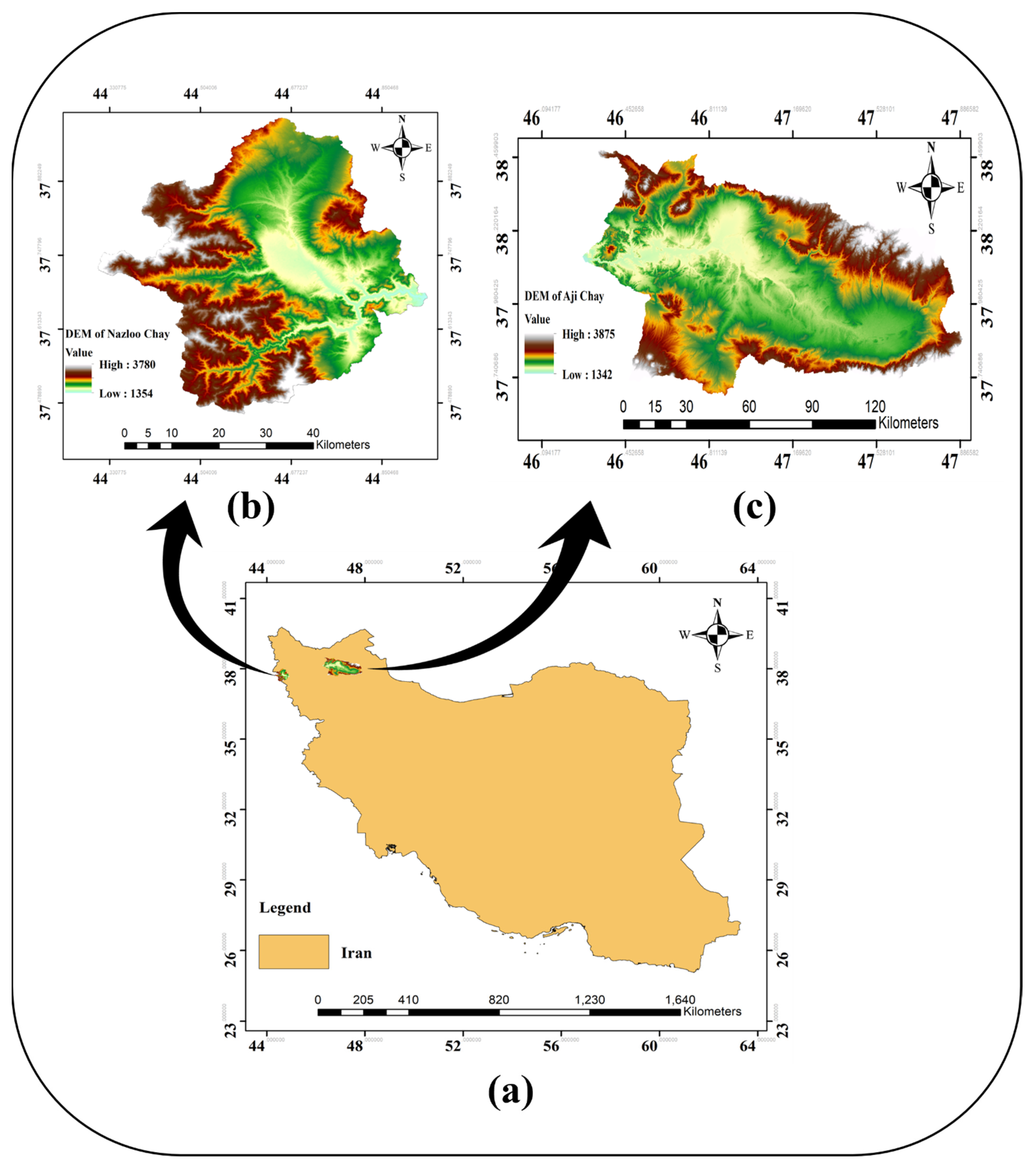
Nowadays, several hydro-environmental systems have faced serious problems due to the impacts of climate change and anthropogenic activities. Located in the northwestern part of Iran, the Lake Urmia basin is a semi-arid region with vulnerable and sensitive ecology. The basin has experienced severe environmental situation, including drought, salt storm, and decreasing groundwater level in the basin. In addition, the lake level (LL) has been rapidly declining over the past decades. Several studies argue that the reduction in the surface water inflow to the lake is the most important reason for the problems [17]. Some other researchers proposed that building a large number of dams over the rivers is the main reason for the problems [18,19]. The researchers started to study this hypothesis due to the extensive construction of reservoirs; however, the hypothesis was rejected in a paper written by Fathian et al. (2014), which showed that decreasing trends were observed in the headwater catchment areas [20]. On the other hand, new publications have found that agricultural activities in terms of increasing crop lands in the region, which has resulted in decreasing inflow to the lake, is the main cause of the decline [21]. While there are different rivers inflowing to the lake, and there has always been a debate between the people who are living in the watersheds on the main reason for the problems, little attention was paid to this question. In addition, vegetation cover changes and their implications and causes are not addressed in the basin.

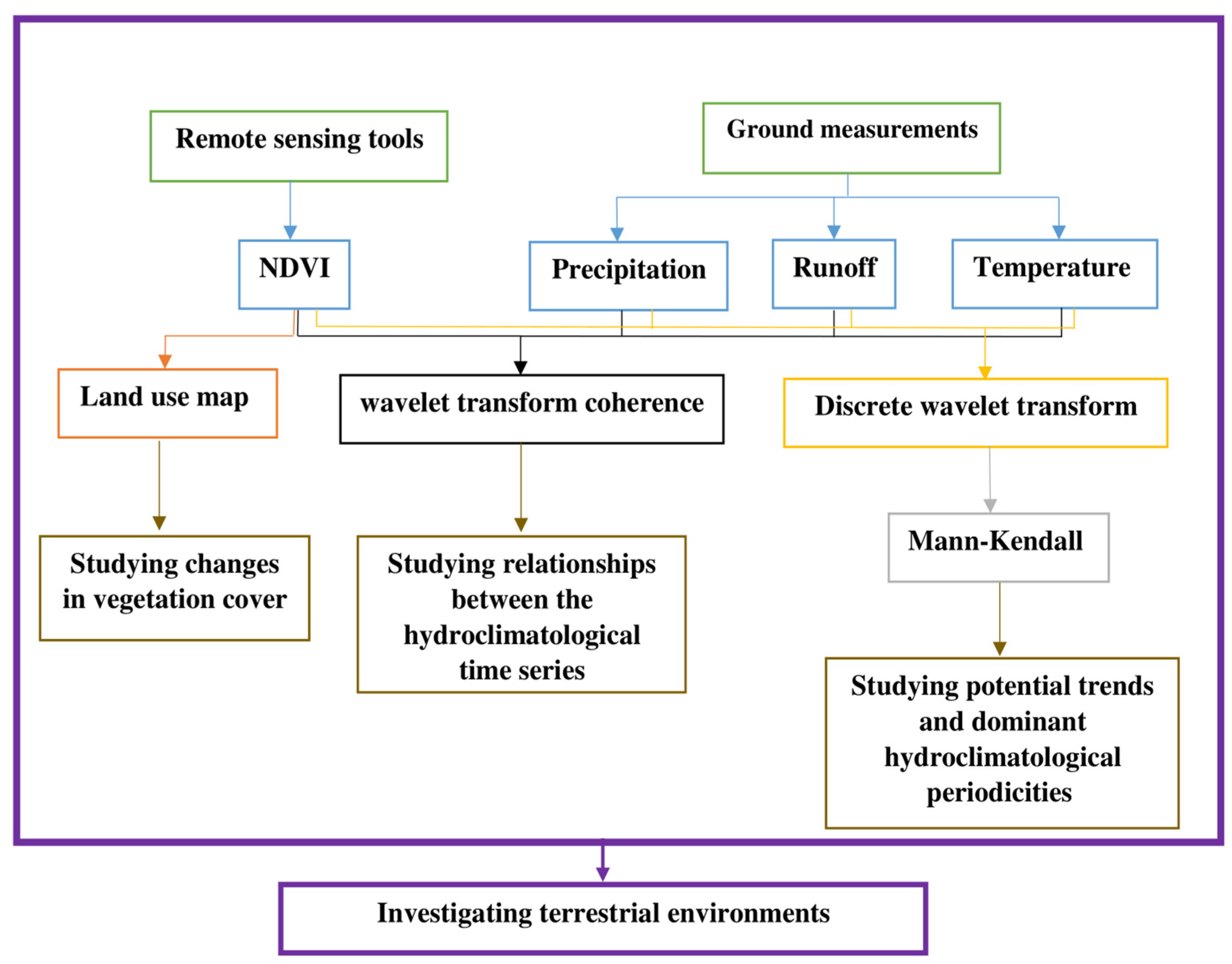
The current study proposed a new methodology to systematically investigate vegetation cover variations, possible drivers and implications of variations, and the connection between vegetation cover, hydro-environmental variables, and human activities in terrestrial environments. Moreover, this study proposed a hydrological methodology to solve a conflict between people. To this end, vegetation cover, hydro-environmental variables, and streamflow across the watersheds of two rivers inflowing to Lake Urmia were investigated using and applying remote sensing tools, the WT technique, trend test analysis, and land use maps.

2. Materials and Methods

2.1. Proposed Methodological Approach

Exploring hydroclimatological patterns and behaviors is crucial in terrestrial environments due to their vulnerability to global and regional cycles and anthropogenic activities. The current study proposed a new methodology to systematically investigate long-term vegetation cover and hydroclimatological changes in terrestrial ecosystems under a changing environment, as presented in Figure 1. To this end, in the first step, the monthly hydroclimatological time series were collected from 1990 to 2020 using remote sensing tools and ground measurements. In the next stage, discrete wavelet transform was employed to decompose the time series into detail and approximation components. After that, the Mann–Kendall trend test was utilized to study potential trends in the time series and determine the most dominant features of hydroclimatological time series in the watersheds. In addition, WTC was used to investigate the relationships between the variables, explore the impacts of climate change and anthropogenic activities on the watersheds, and to find out the significant reasons for pattern change in vegetation cover. In the final stage, the averaged NDVI maps were calculated with 10-year intervals and the pixel value change detection maps between the averaged NDVI maps were collected. In addition, land use maps were generated based on the NDVI maps for 1990, 2000, 2010, and 2020 via SVM to have a deeper insight into the effects of human activities on the watersheds.

2.2. Case Study

Lake Urmia, located between 37°4′–38°17′ latitude and 45°13′–46° longitude in northwestern Iran, was the second largest saline lake on Earth before September 2010 (Figure 2). During the past years, one-fourth of the lake has changed to salt marshes. The lake lost 7 m of its level from 16 m from 1992 to 2018 [22]. There has always been a conflict on the problem between the two provinces located in the western and eastern zones of the lake (East Azerbaijan and West Azerbaijan). The current study selected the Aji-Chay and Nazloo-Chay rivers, located in East Azerbaijan and West Azerbaijan, respectively (the primary inflows to the lake from each province), and their watersheds, as a case study to tackle the conflict.

The Aji-Chay (AC) watershed, located between 37°24′–38°3.7′ latitude and 45°30′–47°45′ longitude, is to the east of Lake Urmia. The river extends 276 km inflow to the lake, and its watershed covers 13853 km² of the Lake Urmia basin. Figure 2 illustrates the DEM map of the watersheds and the rivers located in northwestern Iran. Aji-Chay is a big source of recharge for the local aquifers, and it carries optimum levels of salinity and sediment to the lake [23]. The Nazloo-Chay (NC) watershed is between 37°92′–37°98′ latitude and 44°23′–44°93′ longitude. The AC and NC watersheds are located in a semi-arid region. The NC watershed has an area of 1980 km², and the river extends 95 km west of Lake Urmia. Aji-Chay and Nazloo-Chay rivers are among the essential sources of water for Lake Urmia.

2.3. Data Collection

The current study used remote sensing tools and ground measurements to collect monthly data (NDVI, temperature, precipitation, and streamflow) for 30 years in two watersheds as terrestrial ecosystems. The sources of each variable are presented in

Table 1. The sources of the utilized data.

Data	Type of Data Source	Time Period	Source of Data
NDVI	Remote sensing	1990–2013	Landsat 5 (ETM)
		2014–2020	Landsat 8 (OLI)
Precipitation	Ground-based measurement	1990–2020	Synoptic stations
Temperature
Streamflow			Hydrometric stations

.

The monthly NDVI time series for each watershed was calculated using images from the Landsat 5 Enhanced Thematic Mapper (ETM) (from 1990 to 2013), and Landsat 8 Operational Land Images (OLI) (from 2014 to 2020), to look into the monthly vegetation changes in the AC and NC watersheds. Among the vegetation indices, NDVI is one of the oldest indices for measuring vegetation fractions. It has been used to study dynamics in vegetation covers, such as forestation, deforestation, crop growth status, and evapotranspiration [2]. The Landsat surface reflectance images were collected and processed using the Google Earth Engine (GEE), selecting those with up to 10% cloud cover in this study. The collections were corrected with illumination/viewing geometry and atmospheric effects employing LEDAPS in the ETM sensor and LaSRC in the OLI sensor [24]. The monthly precipitation and temperature time series have been provided by the Iran Meteorological Organization (IRIMO, 2007) in one synoptic station for each watershed. The length of the record started from 1970 with monthly temporal resolution [25]. In order to study the interactions between vegetation cover fluctuations and streamflow, the monthly streamflow dataset of the hydrometric station in NC (Tapik station) and two hydrometric stations in AC (Akhola and Markid stations) were collected from IRIMO. The spring season in Iran is defined as April–May–June, the summer season as July–August–September, the autumn season as October–November–December, and the winter season as January–February–March. The annual and seasonal time series of the variables were also generated by averaging the monthly time series.

2.4. Discrete Wavelet Transform

Wavelet transform uses high and low pass filters, and mother wavelet to decompose a signal into multiple scales. WT analyzes time series and shows numerous features of data at disparate frequencies [26]. Discrete wavelet transform (DWT) decomposes a time series into the approximation (using a low-pass filter) and detail components (using a high-pass filter).

The most critical steps in using DWT are to choose the appropriate decomposition level and the best mother wavelet. It is suggested to select a mother wavelet based on the similarity between the shape of a mother wavelet and the shape of the given time series in time domain [27]. The current study used the Daubechies function to cover different parts of a hydrologic time series [26]. As the first step, the time series were decomposed using DWT in different levels. Then, different smooth Daubechies mother wavelets were utilized for each time series to determine the best fitting function to extract the approximation and detail components of the time series. The most appropriate decomposition level depends on the number of samples in a time series and the chosen mother wavelet. It is suggested to determine the level (L) as follows [28]:

$$L=\frac{\log \left(\frac{n}{2v-1}\right)}{\log 2}$$

(1)

where v stands for the vanishing moments of the mother wavelet, and n is the number of samples in the time series.

In order to study potential trends in hydroclimatological time series and determine the most dominant periodicities, all monthly time series were decomposed into five components (four levels of decomposition), including four detail sub-signals and one approximation subseries. The detail subseries, which show high-frequency components as rapidly changing attributes of the original time series, contain D1 (two-month periodicity), D2 (four-month periodicity), D3 (eight-month periodicity), and D4 (sixteen-month periodicity), and one approximation component (A4), which shows the long-term trend of the time series. Seasonal time series were also decomposed by four levels of decomposition, where the final results contain D1 (six-month periodicity), D2 (twelve-month periodicity), D3 (twenty-four-month periodicity), and D4 (forty-eight-month periodicity) as detail sub-signals, and A4 as the approximation component. Moreover, annual signals were decomposed into four components containing D1 (two-year period), D2 (four-year period), D3 (eight-year period), and A3 (the approximation sub-signal). The decomposition levels were acquired using Equation (1). The approximation components indicate the larger scale or lower frequency attribute of the original time series and likely trend in the time series. The higher level D components have lower frequencies to show the slowly changing behaviors, and lower level D components have higher frequencies to present quickly evolving behaviors. The approximation component is an indicator of the general trend in the primary data.

2.5. Mann–Kendall Trend Test

The Mann–Kendall test is a well-known trend test analysis used in various fields of study, which was selected since no specific statistical distribution is needed to use the trial. The original version of the test (MK1) is used to study the time series with no significant autocorrelation [26]. High positive and low negative MK statistics denote statistically significant increasing and decreasing trends, respectively. The null hypothesis of no trend in the MK test is not acceptable, provided that it is rejected when the probability value becomes less than the predefined significant level (here, $\alpha =5\%$) or greater than the confidence level (95%) [29].

The result of the trend analysis may be misguided if the time series contains significant autocorrelation and seasonal patterns [14]. In this study, the Lag-1 autocorrelation coefficient is used to examine the significance of autocorrelation. If the dataset includes a significant autocorrelation, the pre-whitening MK (MK2) test is used, by which, at first, the autocorrelation is removed from the time series before the MK test is applied.

The correlation coefficient (CC) and Z-MK were utilized in the current study to find out the dominant periodicities of the time series. The sub-signal with a closer Z-MK to the original time series and the highest CC with the original signal reveals the most significant hydroclimatological frequency component in the watershed. The results of this section present baseline information that can be integrated into models, plans, and designs for sustainable management in the future.

2.6. Wavelet Transform Coherence (WTC)

The correlation between the hydroclimatological factors and LL in this study is analyzed using WTC to examine the change characteristics of two given time series and investigate coupled oscillations in both time and frequency domains.

The WTC is a valuable tool to study non-stationary variances and is defined as the square of the cross-spectrum of two given time series, normalized by the individual power spectra [30]. The WTC provides a quantity between 0 and 1 and is used to reflect the direction and the degree of correlation between the hydroclimatological variables and LL. The 1 value indicates a robust linear correlation, and if 0 occurs, it shows that there is no extensive relationship between the signals. In the current study, the Morlet wavelet function was used in WTC analysis due to its applicability for hydrological and climatological time series [31]. WTC explores the coherency between two cross wavelets in both time and frequency domains to measure the intensity of covariance between two time series.

The Monte Carlo method was also utilized in the current study to estimate the statistical significance level of the WTC, which uses statistical models and random samples to find the operations of complicated systems [30]. Additionally, WTC provides helpful information about phase differences between the mutual dominant periodicities of the given time series.

2.7. Support Vector Machine (SVM)

SVM was utilized in this study as a supervised classifier because it can confidently perform the task due to the nonlinear kernel in its structure. The SVM employs the Gini index to measure inequality and this classifier minimizes the classification error in the unseen dataset [32]. In this study, the machine learning SVM is applied to produce classification results. To this end, NDVI images time series generated by Landsat for each watershed were used as the input data for classification [33,34]. The study areas were classified into two classes, as follows: 1. cropland; 2. other types. The output and performance of SVM are highly dependent on the variables in its structure, which are regulated by trial and error [35].

The validation samples were collected from three sources, as follows: (1) general maps provided by the Lake Urmia Restoration Program (LURP); (2) visual interpretation of Google Earth high-resolution images; (3) field surveys. The assessments of accuracy of the obtained maps by SVM were conducted using the confusion matrix and kappa coefficient as performance criteria. The confusion (error) matrix consisted of a cross-tabulation that compares the mapped class labels with the ground truth data [36]. The kappa coefficient (k) represents the difference between the actual agreement and the agreement expected by chance, which ranged from −1 to +1. The values below 0 mean that there is no agreement between the observed and the expected data, a value of 0 indicates an agreement obtained by random choices, and a value of 1 reflects a perfect agreement between the data [36].

3. Results and Discussion

The current study aimed to systematically investigate the spatial–temporal changes in vegetation cover and hydroclimatological time series and their connection to study two river watersheds under changing environments.

Spring (April–June) had the best vegetation cover, and winter (January–March) showed the lowest mean NDVI. Moreover, the NC watershed had more precipitation than the AC one, which has direct effects on vegetation cover. AC’s mean streamflow was almost the same in both Markid and Akhola stations, showing that anthropogenic activities did not affect the AC’s streamflow between the stations. The NC’s average volume of streamflow was much larger than AC’s streamflow. In general, the NC watershed had better hydrologic and environmental conditions.

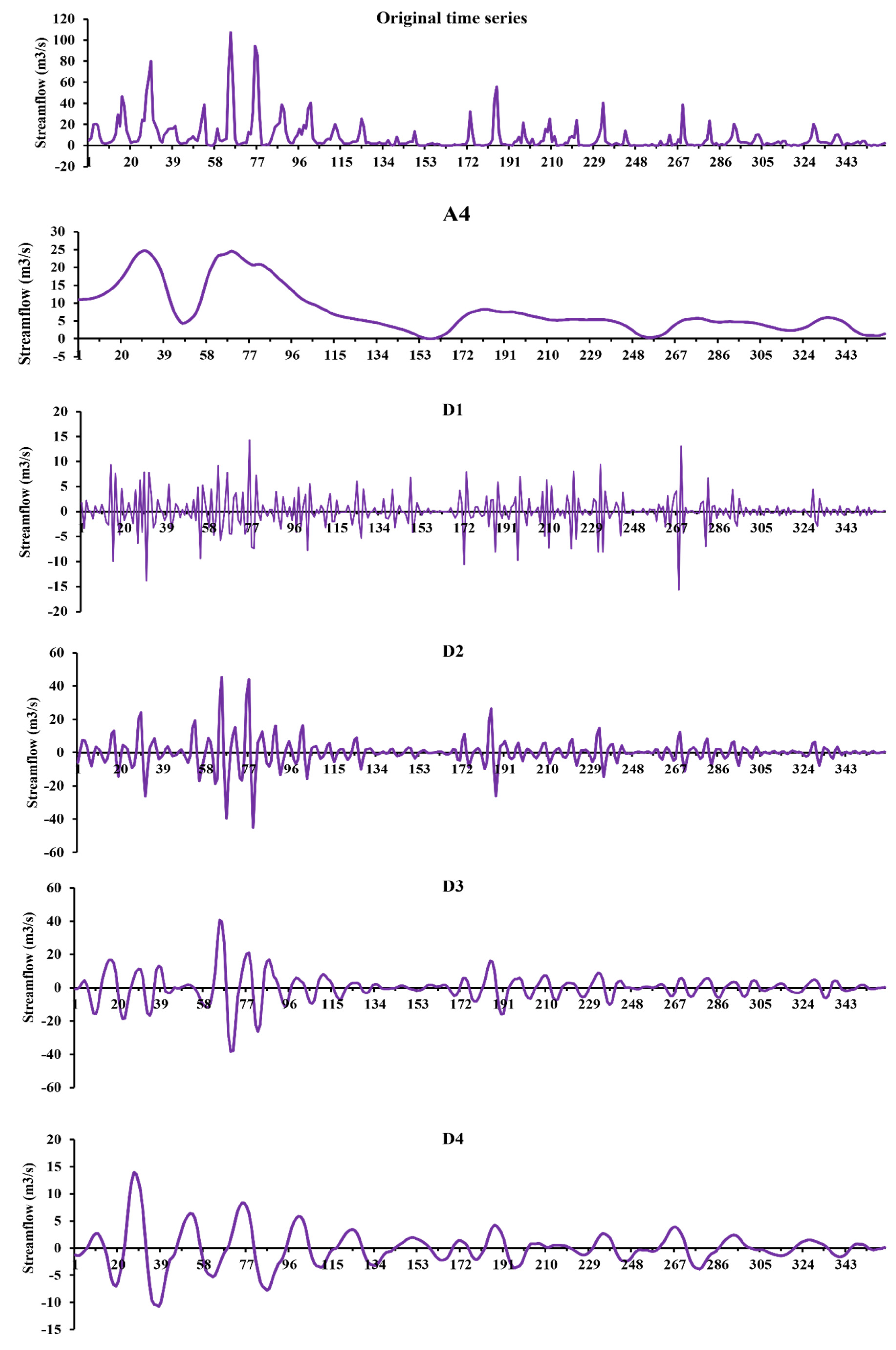
In the first step, DWT was employed to decompose the time series into their approximation and detail components. The approximation and detail components of the monthly streamflow time series measured at Akhola station (in AC) using the db8 mother wavelet and 4 levels of decomposition are shown in Figure 3. Notably, all results are not presented here due to space limitations but the decomposition figures of precipitation, and temperature time series in the AC watershed are presented in Supplementary Materials Figures S1 and S2, respectively.

DWT decomposes time series into different components (Figure 3) with different frequencies. The A component represents the primary trend in the time series, and the D components represent the sub-signals with higher frequency. The detail components show fluctuations, and they are not time series. Therefore, the approximation component should be added to the detail sub-signal to convert it into time series for determining the most dominant periodicities. To this end, different combinations of monthly, seasonal, and annual components were used to produce new generations of subseries. Then, the MK test was applied to determine potential trends in datasets. In this case, the autocorrelation properties of each time series were analyzed using correlograms. For example, the correlograms of temperature and precipitation time series in both watersheds are presented in Figure 4.

The precipitation and temperature time series had the highest autocorrelation with a 12-month period (see the correlogram of the temperature and precipitation time series in Figure 4). This shows that the values of temperature and precipitation are strongly correlated with their own values in the same month of the past year (Lag-12), indicating that hydrological variables contain high seasonality and periodicity. This fact illustrates the demand for multiresolution analysis of hydrological and climatological time series via robust analyzing tools. To this end, in the next stage, the WTC was employed to investigate the connection and correlation between different time series. In the final step, land use maps were generated for 1990, 2000, 2010, and 2020, to explore the area of croplands and agricultural expansion in the watersheds.

3.1. Results of Discrete Wavelet–Mann–Kendall Analysis

After decomposing the original time series, the autocorrelations of the time series were computed, and the appropriate MK test was used to investigate potential trends in original, approximation, detail, and new generation time series. All of the monthly time series indicated high Lag-1 autocorrelation due to the nature of the hydroclimatological variables.

Table 2. Mann–Kendall Z-values and correlation coefficients of monthly time series—Nazloo-Chay.

Streamflow		Precipitation		Temperature		NDVI
CC	Z-MK	CC	Z-MK	CC	Z-MK	CC	Z-MK	Data
	−0.51		−1.98 *		1.8		0.2	Original
0.26	−1.70	0.25	−2.23 *	0.07	3.09 *	0.12	1	A4
0.31	0.56	0.62	−1.35	0.18	2.57 *	0.23	0.3	D1
0.61	2.18 *	0.5	−0.87	0.16	0.95	0.29	−0.2	D2
0.68	−0.14	0.45	−0.54	0.93	0.52	0.88	−0.4	D3
0.21	−0.20	0.34	−0.59	0.29	−0.05	0.27	−0.6	D4
0.49	−3.19 *	0.58	−2.69 *	0.24	2.14 *	0.29	0.7	A4 + D1
0.61	−1.19	0.77	−2.29 *	0.14	2.52 *	0.84	0.4	A4 + D2
0.67	−1.86	0.77	−3.22 *	0.86	1.65	0.48	0	A4 + D3
0.48	−1.38	0.66	−3.44 *	0.57	3.74 *	0.16	1.3	A4 + D4
0.57	−1.08	0.75	−1.67	0.27	2.52 *	0.85	−0.1	A4 + D1 + D2
0.68	−1.79	0.7	−2.17 *	0.83	1.62	0.52	−0.2	A4 + D1 + D3
0.64	−1.61	0.57	−2.00 *	0.62	2.63 *	0.79	0.5	A4 + D1 + D4
0.72	−0.79	0.81	−1.12	0.62	1.24	0.39	−0.2	A4 + D2 + D3
0.65	−1.41	0.82	−2.32 *	0.61	5.02 *	0.94	0.6	A4 + D2 + D4
0.67	−1.87	0.86	−4.63 *	0.98	2.96 *	0.77	0.1	A4 + D3 + D4
0.77	−0.68	0.83	−1.53	0.85	1.24	0.41	−0.2	A4 + D1 + D2 + D3
0.63	−0.97	0.87	−2.01	0.62	32.92 *	0.93	0.7	A4 + D1 + D2 + D4
0.72	−1.79	0.78	−2.39 *	0.99	2.40 *	0.98	0.1	A4 + D1 + D3 + D4
0.92	−0.80	0.9	−1.25	0.99	1.97	0.29	−0.1	A4 + D2 + D3 + D4

* The values with stars (*) have statistically significant trends.

presents the results of MK tests with a 95% significance level for the variables with a monthly time horizon in the NC watershed.

Table 3. Mann–Kendall Z-values and correlation coefficients of seasonal time series—Nazloo-Chay.

Streamflow		Precipitation		Temperature		NDVI
CC	Z-MK	CC	Z-MK	CC	Z-MK	CC	Z-MK	Data
	−0.78		−1.71		1.69		0.3	Original
0.2	−2.96 *	0.27	−1.53	0.11	4.34 *	0.06	5.12 *	A4
0.51	1.75	0.8	0.49	0.12	−1.02	0.97	−0.13	D1
0.84	−0.31	0.36	0.94	0.97	0.31	0.13	−1.94	D2
0.17	−0.68	0.32	−0.16	0.16	−0.20	0.15	0.1	D3
0.24	−0.89	0.2	0.95	0.08	−1.48	0.07	−0.41	D4
0.62	−3.11 *	0.75	−5.08 *	0.46	3.83 *	0.67	0.81	A4 + D1
0.78	−1.10	0.46	−1.54	0.72	2.19 *	0.11	1.99 *	A4 + D2
0.36	−2.41 *	0.41	−1.84	0.5	4.46 *	0.36	2.69 *	A4 + D3
0.52	−2.04 *	0.38	−1.82	0.49	9.36 *	0	3.99 *	A4 + D4
0.45	−0.45	0.68	−1.56	0.85	1.51	0.74	0.55	A4 + D1 + D2
0.62	−4.16 *	0.77	−2.07 *	0.43	3.60 *	0.8	0.36	A4 + D1 + D3
0.74	−1.46	0.78	−2.23 *	0.41	3.06 *	0.79	0.71	A4 + D1 + D4
0.77	−1.18	0.5	−2.02 *	0.78	2.21 *	0.47	1.57	A4 + D2 + D3
0.84	−1.28	0.51	−1.76	0.73	1.95	0.25	1.4	A4 + D2 + D4
0.45	−1.39	0.49	−2.01 *	0.53	4.05 *	0.42	2.49 *	A4 + D3 + D4
0.49	−0.54	0.86	−1.77	0.9	1.77	0.87	0.4	A4 + D1 + D2 + D3
0.88	−0.75	0.85	−1.41	0.9	1.26	0.81	0.52	A4 + D1 + D2 + D4
0.73	−1.10	0.82	−1.89	0.43	2.98 *	0.73	0.33	A4 + D1 + D3 + D4
0.83	−1.32	0.39	−1.54	0.78	1.54	0.59	0.79	A4 + D2 + D3 + D4

* The values with stars (*) have statistically significant trends.

and

Table 4. Mann–Kendall Z-values and correlation coefficients of annual time series—Nazloo-Chay.

Streamflow		Precipitation		Temperature		NDVI
CC	Z-MK	CC	Z-MK	CC	Z-MK	CC	Z-MK	Data
	−1.19		−1.78		2.18 *		0.4	Original
0.35	−2.58 *	0.62	−0.67	0.53	4.03 *	0.27	2.51 *	A3
0.55	0	0.54	0.66	0.72	0.51	0.56	0.13	D1
0.74	−2.50 *	0.66	−1.09	0.37	−0.59	0.83	−0.30	D2
0.32	1.21	0.6	0.13	0.44	0.94	0.07	−1.29	D3
−0.01	−1.98 *	0.92	−1.19	0.68	2.18 *	0.39	1.39	A3 + D1
0.71	−2.44 *	0.44	−1.98 *	0.76	6.87 *	0.7	0.99	A3 + D2
−0.18	−2.40 *	0.54	−0.27	0.73	2.72 *	0.24	1.16	A3 + D3
0.37	−1.58	0.83	−1.68	0.9	1.88	0.97	0.79	A3 + D1 + D2
0.25	−1.39	0.81	−0.69	0.67	2.18 *	0.35	1.19	A3 + D1 + D3
0.91	−1.06	0.49	−2.18 *	0.88	4.08 *	0.7	0.69	A3 + D2 + D3

* The values with stars (*) have statistically significant trends.

present the MK test results for seasonal and annual time scales, respectively, for the NC watershed data.

The results presented in Table 2, Table 3 and Table 4 revealed that the vegetation cover over the NC watershed has almost stable conditions because the NDVI time series in the NC watershed did not show a statistically significant trend. A4 + D2 (4-month periodicity) has the closest Z-MK to the original signal and also the highest CC of all the components. This shows that the most dominant periodicity in the NC watershed is a 4-month periodicity, with no significant trend either. Seasonal and annual time scales did not contain substantial trends. The dominant periodicities for seasonal and yearly horizons were 6-month and 4-year periodicities, respectively.

The monthly and seasonal temperature time series in the NC watershed did not show notable trends (Table 2 and Table 3), and the most dominant periodicities were 8-month (A4 + D3), and 12-month periodicities (A4 + D2), respectively. However, the annual temperature time series indicated a statistically significant increasing trend in the NC watershed, and the 2-year periodicity was the most dominant frequency.

The MK test results for the monthly precipitation time series (Table 2) in the NC watershed indicated a statistically significant decrease in the original signal. The 4-month periodicity (A4 + D2) was the most dominant precipitation periodicity in the watershed. Seasonal and annual horizons did not contain significant trends (Table 3 and Table 4). The periodicities with 48-month and 2-year frequencies (where the results focused on the same periodicity) were the most dominant precipitation periodicities in the NC watershed.

The streamflow time series of NC did not experience a statistically significant trend in monthly, seasonal, and annual time scales (Table 2, Table 3 and Table 4); however, it contains a decreasing trend. The most dominant streamflow periodicities were 8-month, 12-month, and 2-year periods, respectively.

The autocorrelation of the original time series, details, approximations, and the new generations of components in the AC watershed were calculated to choose the appropriate MK test for each time series. The results of the MK tests with a 95% significance level for the time series with monthly, seasonal, and annual time scales in the AC watershed are tabulated in

Table 5. Mann–Kendall Z-values and correlation coefficients of monthly time series—Aji-Chay.

Streamflow (Akhola)		Streamflow (Markid)		Precipitation		Temperature		NDVI
CC	Z-MK	CC	Z-MK	CC	Z-MK	CC	Z-MK	CC	Z-MK	Data
	−0.23		0.11		0.41		1.3		0.96	Original
0.29	−3.44 *	0.27	−3.44 *	0.13	0.57	0.09	2.45 *	0.5	2.88 *	A4
0.53	1.96 *	0.43	1.58	0.61	−0.50	0.22	0.34	0.33	−0.30	D1
0.54	−0.11	0.66	−0.20	0.53	−0.40	0.2	0.68	0.48	0.46	D2
0.58	−0.10	0.51	0.12	0.52	0.07	0.94	0.47	0.43	−0.19	D3
0.31	−0.13	0.15	1.61	0.24	0.12	0.18	0.77	0.51	−0.57	D4
0.67	−2.22 *	0.29	−3.68 *	0.17	0.14	0.2	1.92	0.86	2.56 *	A4 + D1
0.66	−2.28 *	0.33	−2.59 *	0.58	0.48	0.28	1.74 *	0.82	2.17 *	A4 + D2
0.77	−3.20 *	0.37	−2.20 *	0.79	1.26	0.91	1.41	0.87	1.9	A4 + D3
0.76	−1.86	0.46	−2.44 *	0.55	0.85	0.46	1.88	0.93	1.22	A4 + D4
0.64	−2.31 *	0.32	−2.12 *	0.4	0.02	0.2	1.27	0.78	1.79	A4 + D1 + D2
0.75	−2.33 *	0.35	−1.40	0.73	0.49	0.94	1.45	0.87	1.8	A4 + D1 + D3
0.75	−2.93 *	0.36	−2.80 *	0.49	0.61	0.55	1.47	0.94	0.99	A4 + D1 + D4
0.75	−1.30	0.44	−0.53	0.8	0.5	0.97	1.25	0.86	1.62	A4 + D2 + D3
0.8	−1.46	0.38	−2.50 *	0.66	0.63	0.52	1.22	0.94	1.48	A4 + D2 + D4
0.81	−1.82	0.38	−1.70	0.86	1.17	0.95	1.51	0.92	1.36	A4 + D3 + D4
0.78	−0.51	0.36	−0.32	0.85	0.22	0.98	1.16	0.84	1.77	A4 + D1 + D2 + D3
0.75	−1.15	0.39	−1.84	0.55	0.36	0.55	1.17	0.97	1.49	A4 + D1 + D2 + D4
0.88	−0.86	0.43	−0.84	0.85	0.47	0.96	1.5	0.94	1.04	A4 + D1 + D3 + D4

* The values with stars (*) have statistically significant trends.

,

Table 6. Mann–Kendall Z-values and correlation coefficients of seasonal time series—Aji-Chay.

Streamflow (Akhola)		Streamflow (Markid)		Precipitation		Temperature		NDVI
CC	Z-MK	CC	Z-MK	CC	Z-MK	CC	Z-MK	CC	Z-MK	Data
	−0.92		−1.13		0.4		1.04		0.78	Original
0.25	−3.50 *	0.25	−4.09 *	0.2	−0.32	0.09	2.49 *	0.18	5.07 *	A4
0.91	−0.65	0.92	0.85	0.68	0.03	0.97	−0.02	0.9	−0.02	D1
0.09	−1.13	0.12	0.54	0.65	0.01	0.2	−1.15	0.35	0.09	D2
0.23	−0.054	0.12	1.09	0.27	−0.12	0.15	−1.33	0.15	0.42	D3
0.2	−0.8269	0.25	0.86	0.07	0.62	0.04	−1.00	0.13	1.03	D4
0.7	−1.447	0.62	−1.82	0.81	0.31	0.9	1.15	0.7	1.38	A4 + D1
0.6	−2.85 *	0.76	−6.12 *	0.8	0.22	0.17	2.49 *	0.52	6.64 *	A4 + D2
0.76	−3.04 *	0.83	−4.69 *	0.59	0.38	0.28	2.57 *	0.29	7.92 *	A4 + D3
0.49	−3.46 *	0.74	−3.35 *	0.75	0.78	0.61	2.72 *	0.38	5.46 *	A4 + D4
0.62	−0.92	0.55	−1.30	0.93	0.09	0.9	1.19	0.89	0.84	A4 + D1 + D2
0.79	−1.48	0.73	−1.73	0.86	0.36	0.89	1.09	0.82	1.3	A4 + D1 + D3
0.77	−1.46	0.94	−1.51	0.86	0.81	0.93	0.91	0.85	1.38	A4 + D1 + D4
0.63	−2.57 *	0.78	−4.21 *	0.84	0.12	0.28	2.27 *	0.55	2.36 *	A4 + D2 + D3
0.52	−3.04 *	0.79	−3.99 *	0.84	0.31	0.42	2.79 *	0.61	3.74 *	A4 + D2 + D4
0.69	−2.53 *	0.79	−3.58 *	0.67	0.64	0.46	2.25 *	0.36	4.21 *	A4 + D3 + D4
0.69	−0.822	0.72	−1.75	0.96	0.32	0.85	1.17	0.94	0.72	A4 + D1 + D2 + D3
0.79	−0.695	0.92	−1.12	0.97	0.48	0.96	1.03	0.96	0.9	A4 + D1 + D2 + D4
0.8	−1.30	0.94	−1.09	0.86	0.5	0.94	0.73	0.89	1.24	A4 + D1 + D3 + D4
0.57	−2.23 *	0.79	−5.80 *	0.87	0.21	0.54	2.08 *	0.7	5.11 *	A4 + D2 + D3 + D4

* The values with stars (*) have statistically significant trends.

and

Table 7. Mann–Kendall Z-values and correlation coefficients of annual time series—Aji-Chay.

Streamflow (Akhola)		Streamflow (Markid)		Precipitation		Temperature		NDVI
CC	Z-MK	CC	Z-MK	CC	Z-MK	CC	Z-MK	CC	Z-MK	Data
	−1.68		−1.78		0.69		1.48		2.67 *	Original
0.62	−3.78 *	0.61	−3.10 *	0.27	2.60 *	0.39	2.80 *	0.67	3.62 *	A3
0.61	−0.86	0.41	−0.19	0.7	0.23	0.84	2.61 *	0.62	0	D1
0.55	0.2	0.7	0.19	0.44	0	0.3	0.29	0.56	0.09	D2
0.61	−1.48	−0.20	1.74	0.58	−0.16	0.26	−0.41	−0.08	−0.68	D3
0.87	−2.08 *	0.86	−3.46 *	0.63	2.44 *	0.61	1.19	0.94	2.87 *	A3 + D1
0.69	−1.98 *	0.99	−3.85 *	0.77	1.48	0.81	5.32 *	0.95	5.76 *	A3 + D2
0.75	−2.60 *	0.93	−2.86 *	0.78	0.46	0.38	1.31	0.91	3.31 *	A3 + D3
0.82	−1.28	0.99	−2.92 *	0.84	0.89	0.95	1.38	0.99	2.77 *	A3 + D1 + D2
0.75	−2.27 *	0.9	−3.26 *	0.89	0.49	0.74	1.187	0.92	2.67 *	A3 + D1 + D3
0.73	−1.98 *	0.97	−3.91 *	0.9	0.43	0.54	1.44	0.95	4.59 *	A3 + D2 + D3

* The values with stars (*) have statistically significant trends.

, respectively.

The monthly and seasonal NDVI time series in the AC watershed did not show significant trends (Table 5 and Table 6). The most dominant monthly and seasonal NDVI periodicities in the AC watershed were 16-month (A4 + D4) and 6-month periodicities, respectively, which showed closer Z-MK to the original time series and also the highest CC among the subseries. However, the results indicated a statistically significant increasing trend in the annual NDVI time series. The most yearly dominant periodicity was a 2-year period.

The temperature time series in the AC watershed indicated an almost stable situation in monthly, seasonal, and annual horizons without significant trends (see Table 5, Table 6 and Table 7). According to Table 5, Table 6 and Table 7, the 8-month (A4 + D3), 6-month (A4 + D1), and 8-year (A3 + D3) periods indicated the most critical impact on the original monthly, seasonal, and annual temperature time series, respectively.

The precipitation time series in the AC watershed did not show a significant trend in the AC watershed in all monthly, seasonal, and annual time scales (see Table 5, Table 6 and Table 7). However, this watershed’s most dominant monthly, seasonal, and yearly precipitation periodicities were 8-month, 12-month, and 2-year periods, respectively.

The Markid station’s time series, as one of the stations to measure AC’s streamflow, showed no significant trend, and the most dominant monthly, seasonal, and annual periodicities for streamflow were 16-month, 6-month, and 4-year periods, respectively (see Table 5, Table 6 and Table 7). There were no statistically significant trends in time series with slightly negative trends. The streamflow time series in Akhola station did not contain any statistically important trends; however, it had a negative trend. The 8-month (A4 + D3), 6-month (A4 + D1), and 2-year (A3 + D1) periods were the most dominant periodicities for monthly, seasonal, and annual time series, respectively, for observed streamflow in the Akhola station.

In the next section of the paper, the WTC results are shown to give a better insight into the complex relationships between the investigated variables due to the multiresolution characteristics of the hydroclimatological and land cover time series.

3.2. Wavelet Transform Coherence Results

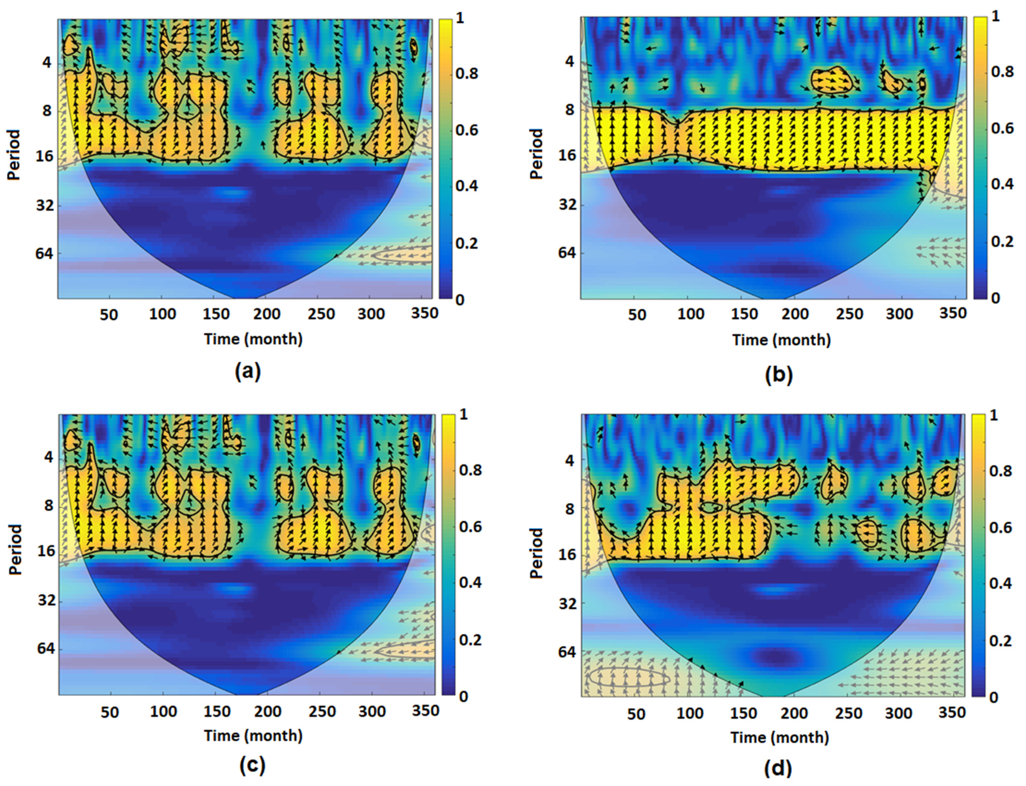
Investigating the main reasons for the changing behaviors of natural time series is complicated due to their multiresolution behavior and, as a result, needs profound elaboration in both the time and frequency domains. The WTC was used in this study to reveal different aspects of the correlation between NDVI and other hydroclimatological variables. The results are presented in Figure 5 and Figure 6. In the WTC plots, the regions surrounded with thick black lines indicate the common periodicities with a strong relationship between the time series at 95% confidence level. In addition, arrows show the types of correlation and phase shift where rightward arrows indicate the in-phase relationship and leftward arrows indicate the anti-phase relationship between two time series. The other important point in the WTC plots is the cone of influence (COI) which shows the region that has not been impacted by the edges of the wavelet spectrum (indicated by the thin black line). Notably, the time series were first standardized to have unit variance and zero mean before applying WTC.

The WTC between monthly NDVI and temperature time series in the NC watershed (Figure 5a) indicates a significant in-phase relationship with 8–24-month frequencies for the entire period. Moreover, a close anti-phase relationship is illustrated with a 6-month frequency. In addition, common periodicities from 2015 to 2020 are illustrated with a 64-month frequency and a 16-month time-lag. The results of the WTC technique (Figure 5b) indicate that monthly NDVI and precipitation time series in the NC watershed had standard frequency in a 12-month period with changing time-lag. There is also a close in-phase relationship from 2014 to 2020 with a 64-month frequency. These findings illustrate that vegetation cover changes might be linked to precipitation. The WTC plot between NDVI and streamflow (Figure 5c) shows a close anti-phase relationship with a 6-month frequency, indicating streamflow as the leader in this relationship. Moreover, common significant periodicities are seen with 8–16-month periods and 2–4-month time-lags. The streamflow time series was the leader from 1990 to 2015; however, an abrupt change was seen which changed the leadership from the streamflow time series to the NDVI time series from 2015 to 2020.

For the AC watershed, the WTC results (Figure 6a) indicate common 6–12-month periodicities with 3–4 months of time-lag between NDVI and measured streamflow at Akhola station. The WTC graph between NDVI and temperature (Figure 6b) illustrates significant common periodicities in 8–16-month frequencies with 4–8-month time-lags from 1990 to 2000 and 2–8-month time-lags from 2000 to 2020. The measured streamflow in the Markid station and NDVI time series had a strong relationship with 8–16-month frequencies and 2–8-month time-lags (streamflow was the leader). The WTC graph between monthly NDVI and precipitation time series in the AC watershed (Figure 6d) indicates a robust relationship at 8–16 months, with 4–8-month time-lag from 1990 to 2005. From 2005, the strength of the relationship declined up to 2010, and after that, the situation came back to the aforementioned time (2005).

3.3. Spatiotemporal Investigation of Vegetation Cover

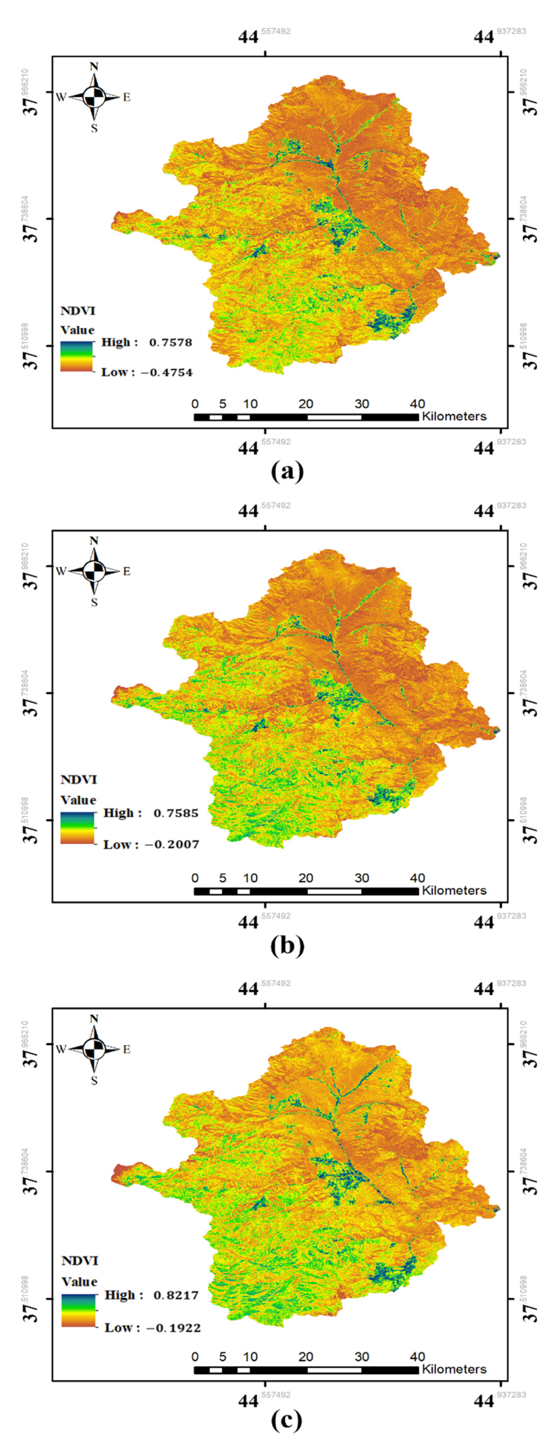
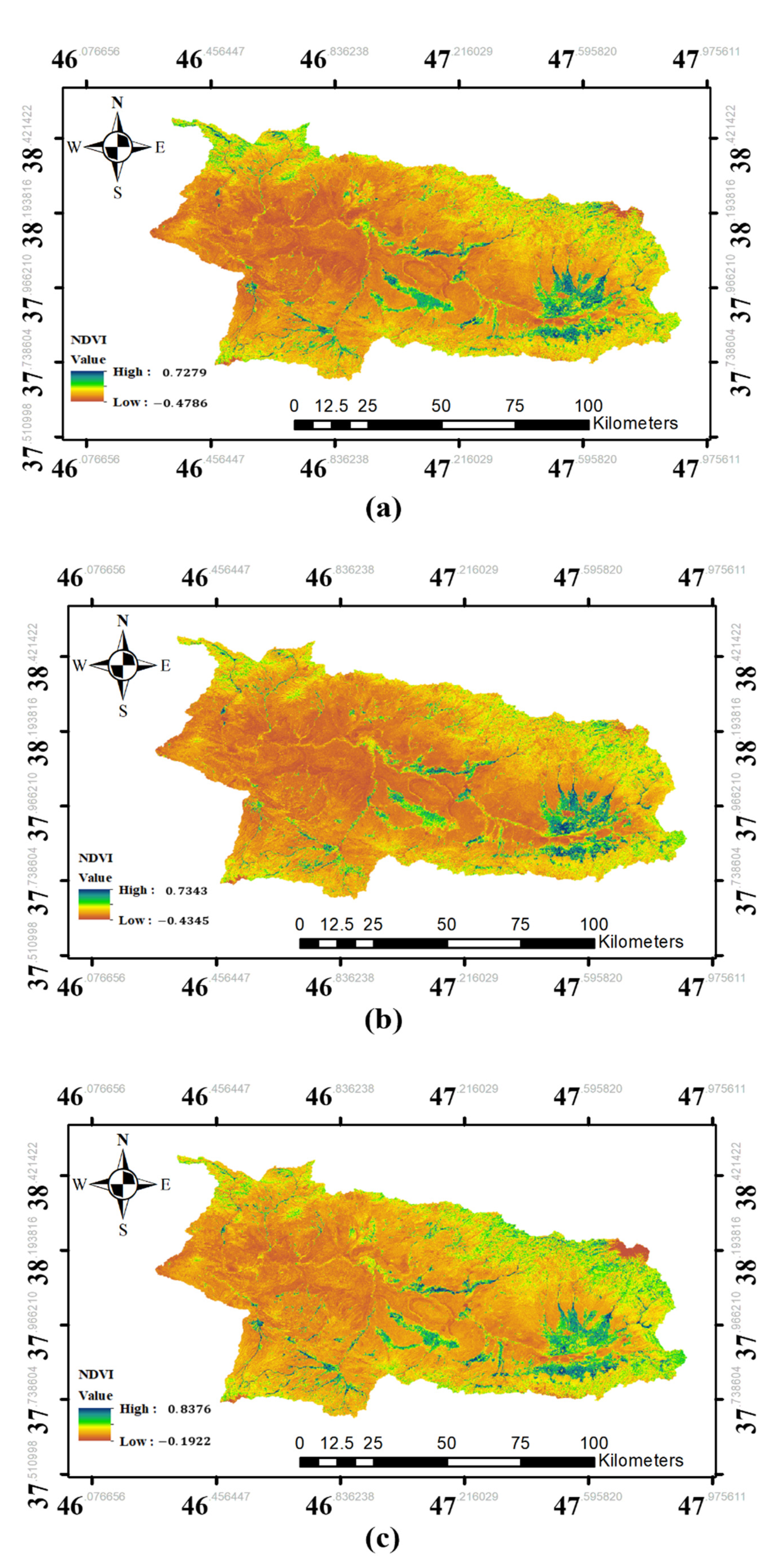
In the final section, spatiotemporal changes in vegetation covers were explored using NDVI maps. To this end, average NDVI maps were generated for 1990–2000, 2000–2010, and 2010–2020 using Landsat 5 and Landsat 7 images in the watersheds to reduce the effects of a sudden unstable change in a year on the analysis. Figure 7 and Figure 8 present the average NDVI maps for the NC and AC watersheds, respectively.

The results (Figure 7) indicated that regions with dense vegetation cover increased (in the western and southern parts of the map) from 1990–2000 to 2000–2010, but the highest NDVI value was almost the same in the NC watershed. In addition, regions with healthy vegetation cover increased from 2000–2010 to 2010–2020; in addition, the highest NDVI value increased.

Figure 8 shows that regions with dense vegetation cover and the highest NDVI value were almost identical from 1990–2000 to 2000–2010 in the AC watershed. After that, areas with healthy vegetation cover and the highest NDVI value increased from 2000–2010 to 2010–2020 in the watershed, especially in the eastern and northern parts. According to the results presented in Section 3.1 and Section 3.2, the AC watershed did not experience more precipitation, and the impacts of human activities were evident in the region. The results indicated that people in the AC watershed cultivated crops with more water demand, and the agricultural lands may have increased in the AC watershed.

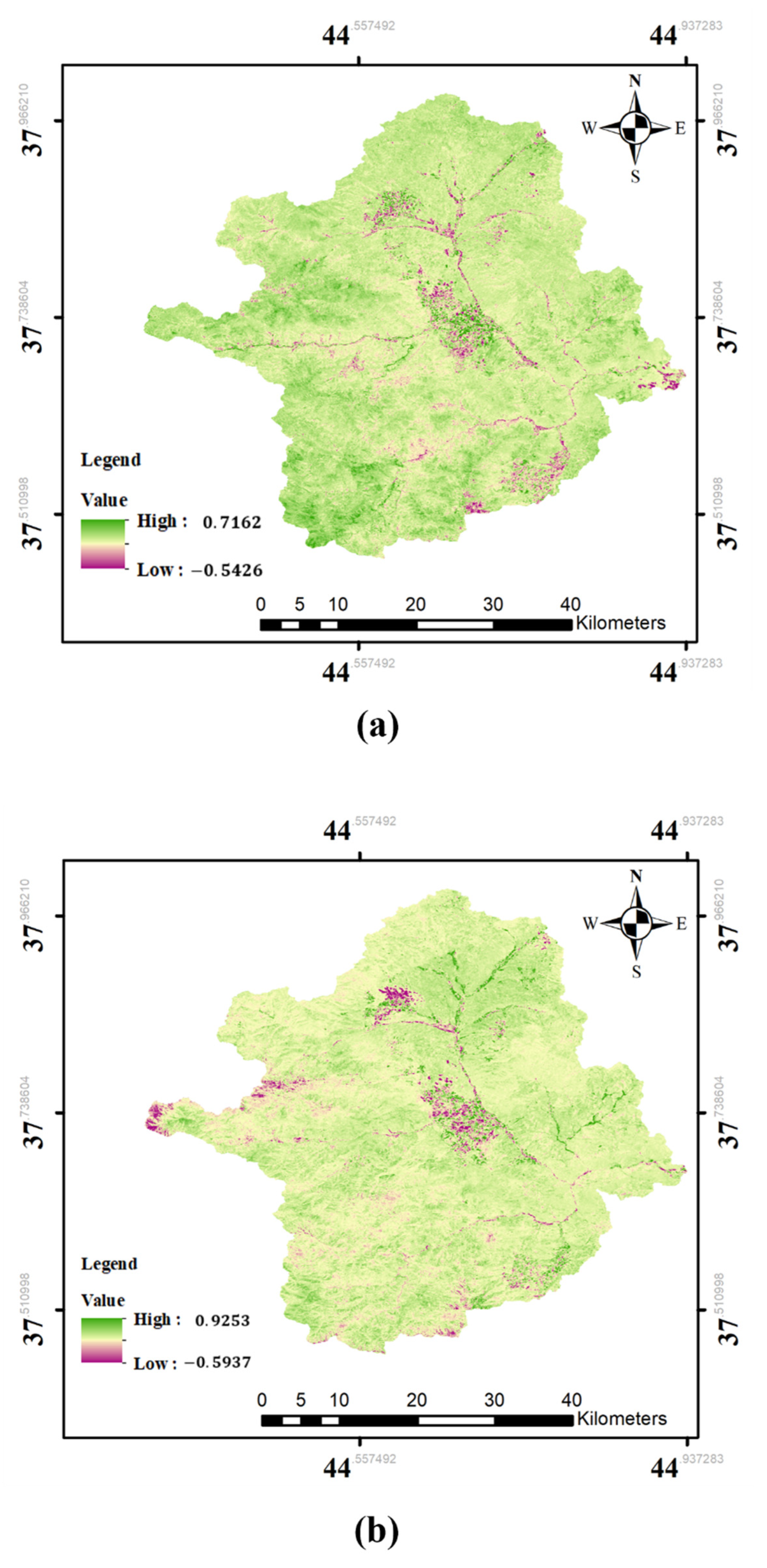
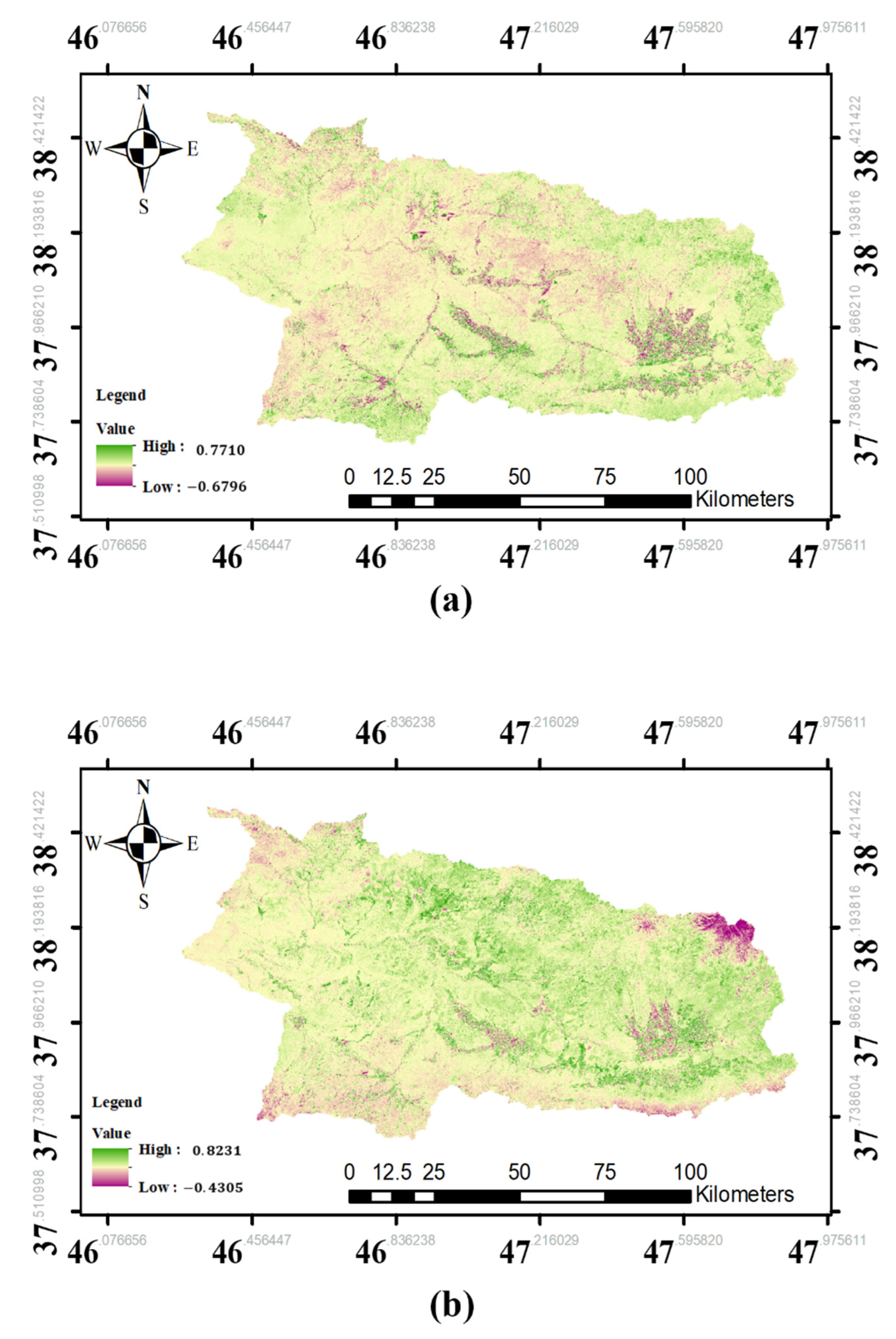
To further investigate the NDVI changes in each pixel, two pixel value change detection maps were generated between the averaged NDVI maps from 1990 to 2000, 2000 to 2010, and 2010 to 2020 for each watershed. The results are shown in Figure 9 and Figure 10 for the NC and AC watersheds, respectively.

The pixel value change detection map between the averaged NDVI maps of 1990–2000 and 2000–2010 in the NC watershed (Figure 9) indicated that the NDVI values increased across the watershed except for some parts in the middle and southeastern parts of the watershed where the NDVI value was decreased. Although, there were several regions that did not experience NDVI change. On the other hand, the NDVI change map between the averaged NDVI maps of 2000–2010 and 2010–2020 in the NC watershed revealed that almost all of the watershed experienced increasing NDVI values. The NDVI growth was stronger in the southern and northern parts of the watershed.

In the AC watershed, the pixel value change detection map between the averaged NDVI maps of 1990–2000 and 2000–2010 (Figure 10) showed that eastern and southern regions of the watershed have experienced increasing NDVI values, but the other parts had almost the same values. Additionally, the NDVI change map between the averaged NDVI maps of 2000–2010 and 2010–2020 in the AC watershed indicated a growing NDVI value in pixel level all over the watershed, except for the western parts, that had almost stable NDVI values, and a small part of the northeastern AC, which experienced decreasing NDVI value.

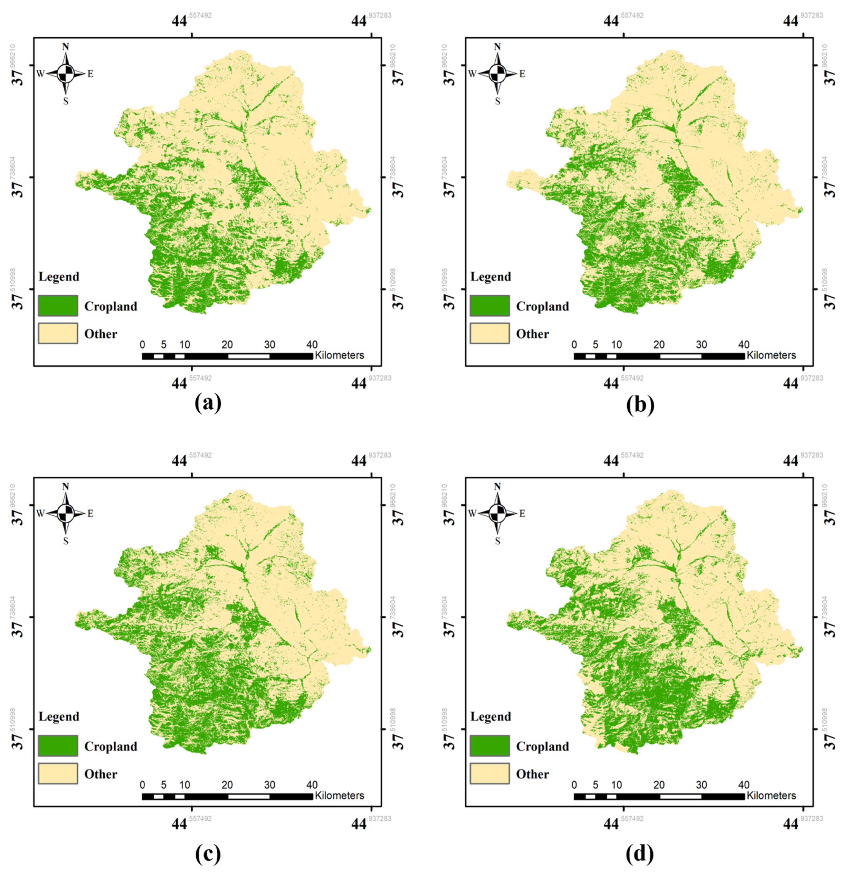
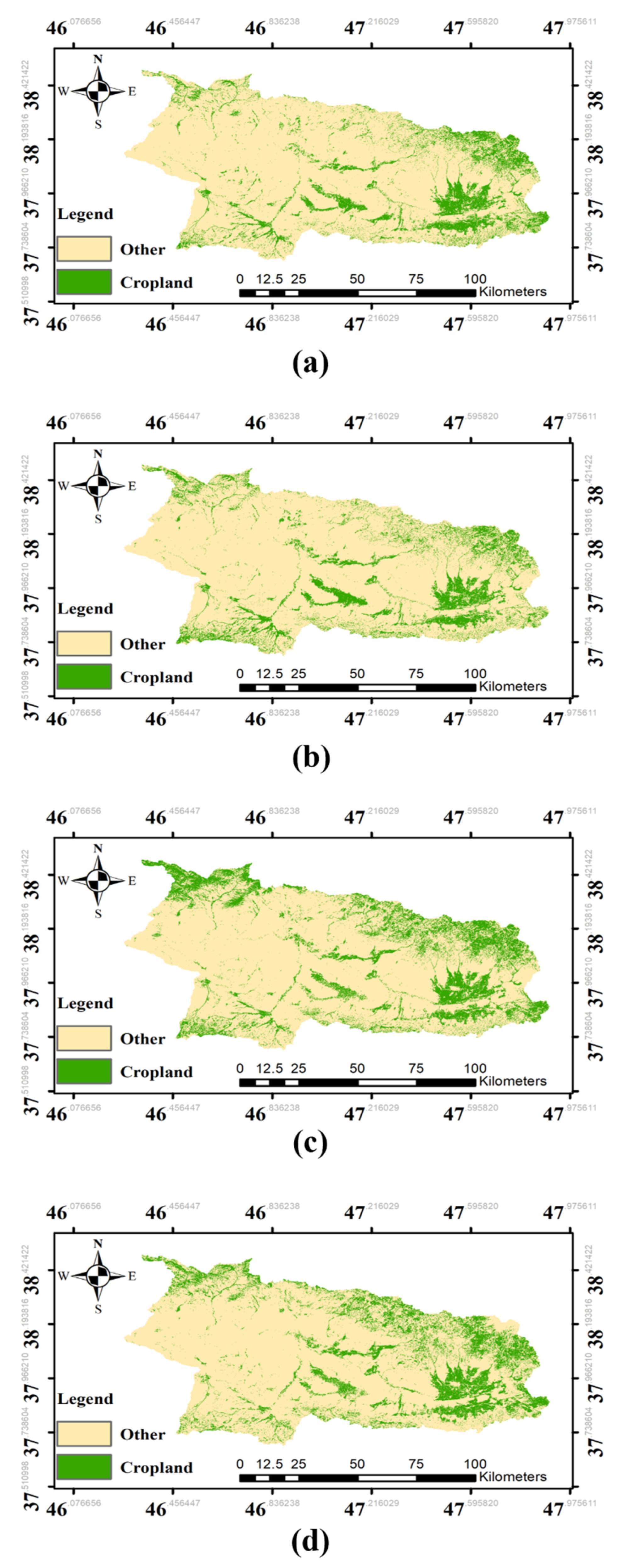
In the next stage, SVM was employed to classify the land use of the NC and AC watersheds into two classes—1. cropland; 2. other—to explore the cumulative agricultural area in the watersheds. To this end, the NDVI maps for years 1990, 2000, 2010, and 2020 were calculated to have a deeper insight into agricultural expansion in both watersheds and SVM was then applied to classify the images to determine the total area of agricultural lands for each year in each watershed. The results are given in Figure 11 and Figure 12 for the NC and AC watersheds, respectively. In addition, the accuracy assessments of results are presented in

Table 8. Mann–Kendall Z-values and correlation coefficients of annual time series—Aji-Chay.

Watershed	Period of Data	Training Sample Points		Validation Sample Points		Overall Accuracy	Kappa Coefficient
		Cropland	Other	Cropland	Other
Ajichay	1990–2000	462	556	202	272	0.7825	0.7691
	2000–2010	519	607	200	300	0.8104	0.7968
	2010–2020	578	634	267	322	0.8882	0.8691
Nazloochay	1990–2000	343	498	197	258	0.8181	0.7913
	2000–2010	401	512	208	273	0.7992	0.7899
	2010–2020	453	591	222	304	0.8521	0.8475

.

According to the land use maps of the NC watershed (Figure 11), the cumulative area for agricultural lands in this watershed were 1077, 1332, 1195, and 1123 km² for 1990, 2000, 2010, and 2020, respectively. The agricultural lands are mainly located in the western and southwestern parts of the watershed. The cropland experienced a 20% increment between 1990 and 2000; after that, the total area decreased 10% between 2000 and 2010. From 2010 to 2020, the NC watershed indicated an approximately stable area for cropland.

The total area of croplands in the AC watershed (Figure 12) were 1182, 1155, 1526, and 1434 km² for 1990, 2000, 2010, and 2020, respectively. The croplands are mainly located in eastern and southeastern parts of the watershed. Although the cumulative area of agricultural lands showed a stable situation from 1990 to 2000, it experienced a significant expansion (about 35%) from 2000 to 2010, which almost stayed in a stable condition up to 2020.

4. Discussion

Generally, the hydroclimatological variables and vegetation cover in the NC watershed and the river’s streamflow were almost stable and indicated no significant trends. The monthly precipitation and annual temperature time series were the sole variables with statistically substantial decreasing and increasing trends, respectively. The positive trend in the temperature time series in the NC watershed can be a reflector of human activities and needs more investigation. Previous studies have shown vegetation dynamics (expressed as NDVI) are strongly correlated with precipitation [37]. In this study, according to the stable situation of vegetation cover when precipitation was decreasing, the relationship between the time series needs more investigation to specify various aspects of connection to determine the impacts of climate change and anthropogenic activities. The observed decreasing trend in streamflow is aligned with the findings of Chaudhari et al. (2018), who demonstrated that the impacts of anthropogenic activities were amplified in the Lake Urmia basin in terms of dam construction and urban and agricultural expansion [38]. In addition, the observed negative trend in precipitation time series has an agreement with the findings of recent publications showing a meteorological drought in the Lake Urmia basin from 1998 to 2002, which resulted in decreasing precipitation for several years [17].

The most dominant periodicities illustrated important terms of hydroclimatological variables in the NC watershed. According to the results, as mentioned earlier, temperature, precipitation, and streamflow demonstrated a common 2-year periodicity. The results for monthly and dominant seasonal periodicities revealed that, although precipitation and streamflow should have close dominant periodicities, vegetation cover time series are the leader in the relationship between the vegetation cover with precipitation and streamflow time series. These results may indicate that humans have affected the watershed, which has impacted the relationship between the variables.

In general, the trend of NDVI time series in the AC watershed increased in stable conditions of precipitation and temperature and decreasing streamflow. The increasing vegetation cover in the AC watershed consistent with reports of agricultural expansion in the Lake Urmia basin [21,39]. The increasing vegetation cover in the situation that precipitation and temperature time series were almost stable suggests that anthropogenic activities in agricultural expansion have occurred in the watershed. This finding is matched with recent articles that showed the agricultural activities have been increasing in the Lake Urmia basin [14]. According to the decreasing trend of streamflow time series, the people living in the AC watershed were using water from Aji-Chay to perform more agricultural activities, leading to less streamflow in the river and decreasing inflow to the lake. It is notable that Alborzi et al. (2018) reported increasing withdrawal of surface water resources in the Lake Urmia basin [21].

The most dominant periodicities that were found in the presented analysis showed important periodicities of the variables in the AC watershed. The main dominant periodicities in the watershed were 6- and 8-month periodicities, and 2-year periodicities, which were common in vegetation cover, temperature, precipitation, and streamflow in both stations. However, natural vegetation cover variations should have a close relationship with precipitation and streamflow with a logical time-lag. The same discussions about the time-lags between NDVI and precipitation time series have been carried out in China and the results indicated the effects of human interventions and climate change [4]. The dominant periodicities of vegetation cover in the AC watershed were 6-month periodicities, while it was 8 month for the precipitation and streamflow measured at Akhola station. Moreover, vegetation cover showed the same dominant periodicity with the streamflow at the Markid station without time-lag, while recent studies have indicated that time-lags between precipitation and vegetation cover responses in a watershed should be expected in normal situation [12,40]. These findings illustrated that the changes in vegetation cover in the AC watershed might be due to human interventions.

To further investigate the relationship between the variables, WTC was utilized in the current study. The results of WTC indicated a close relationship between temperature and vegetation time series in the NC watershed, which suggests that temperature has a remarkable impact on vegetation cover variations in the NC watershed. The WTC results revealed a changing pattern in time-lags between NDVI and precipitation time series. The abrupt change in the direction of the relationship could indicate high anthropogenic activities in the region. Previous studies have used simple correlation analysis to study the linkage between the variables. Therefore, they did not have good insight into the changing pattern of the relationships over a period of time. The sudden change in the role of the leading variable between NDVI and streamflow in the NC watershed in 2015 is an indicator of anthropogenic activities in the NC watershed. Unsurprisingly, the close relationship between NDVI and streamflow suggests that streamflow has remarkable impacts on the vegetation cover in the NC watershed.

Generally, the common periodicities with the stable directions between the NDVI and streamflow time series in the Akhola station in the AC watershed indicate that the vegetation cover changes depend on the streamflow measured at the Akhola station without human interventions. The smooth change in the direction of common periodicities between vegetation cover and temperature time series in the AC watershed reveals the impact of climate change on the weather of the watershed. This finding is aligned with the results of Section 3.1 that indicated a non-significant increasing trend in the temperature time series in the AC watershed.

The current study investigated the NDVI maps to study the spatial vegetation cover changes in the watersheds. A watershed will have a healthier vegetation cover when the region has more available water or the crop species change. According to the results of Section 3.1 and Section 3.2, none of the watersheds had better environmental conditions during the past 30 years; therefore, it could be concluded that the increasing and decreasing density of vegetation cover in the watersheds have anthropogenic causes. These findings denote that the types of crops cultivated by people have been changed to crops that require more water. This finding is aligned with previous studies in different parts of the basin [41]. To delve deeper into the spatial changes of NDVI maps, the pixel value change detection maps were explored in the watersheds. The results revealed that the NDVI values have been increased in both watersheds, especially those averaged results from 2000–2010 to 2010–2020, which are an indicator of crop species with more water demand. These findings are in alignment with the results presented by Hesami et al. (2016) indicating that the water demand for agricultural activities are increased in the Lake Urmia basin [41]. According to the results provided in Section 3.1 and Section 3.2, the streamflow in the NC river had almost no change, and the precipitation decreased in the watershed, which indicates that the water acquired from river or precipitation was not the main source for excessive water usage; therefore, to change the crop types, people might use groundwater resources. Previous studies have reported groundwater depletion in the Lake Urmia basin over the past decades, which supports the discussions made in this section of the study [42,43].

Using land use maps, the current study aimed to explore the expansion of agricultural areas in the case studies. Generally, after increasing agricultural activities from 1990 to 2000, the area of cropland declined in the NC watershed, which could be due to sustainable water resources management in the region and/or the decrement in groundwater level induced by excessive utilization. In a nutshell, the NC watershed contained the same area of agricultural lands in 1990 and 2020. Therefore, this did not indicate continuous agricultural expansion, rather it indicated that the area experienced agricultural growth in a limited period.

According to the results presented in Section 3.1, the measured streamflow in both the Markid and Akhola stations indicated a slight decrement which was not statistically significant. At the same time, 35% agricultural expansion would need a significant excessive amount of water. Moreover, the precipitation time series did not experience a significant increasing trend in the AC watershed. Therefore, groundwater was used for more agricultural activities in this region. Thus, from a general point of view, the agricultural activities have experienced a significant expansion in the AC watershed with excessive groundwater usage. This finding is aligned with the results of previous sections suggesting that human activities have harmfully impacted the watersheds.

5. Conclusions

Monitoring vegetation cover and hydroclimatological variables under changing environments is very important for water resources and environmental management. The current study focused on the watersheds of two rivers, Aji-Chay and Nazloo-Chay, in Iran, which are among the inflows to Lake Urmia, which is the second largest saltwater lake on Earth. There have been many conflicting discussions between the people of the watersheds regarding the LL decline of Lake Urmia.

Determining the most dominant hydrological and environmental periodicities in the watersheds is crucial for management purposes. The hydroclimatological variables have different attributes; however, a general conclusion indicates that 8-month, 6-month, and 2-year periodicities are the most dominant periods in the NC and AC watersheds. The results indicated that the most dominant periodicities of vegetation cover, precipitation, and streamflow logically denote the anthropogenic activities in the watersheds, especially the AC watershed.

The hydroclimatological variables were almost stable in the watersheds, indicating that climate change did significantly impact on the region. Overall, the results showed that the vegetation cover increased in both watersheds, though without a statistically significant trend in the NC watershed. According to the stable environmental situations in the region, decreasing or stable amounts of streamflow should result in reduced vegetation cover; however, in the Lake Urmia basin (in both NC and AC watersheds), the reverse was true. The investigation of changing points in the mutual periodicities, directions, and time-lag between vegetation cover and hydroclimatological time series also indicated that the people of both watersheds utilized groundwater to increase their activities. In addition, the cultivated crops in both watersheds have been changed to crops which require excessive water utilization. One of the limitations in this study was the access to ground-based crop type classification data to generate a detailed land cover map. It will be helpful to explore the crop type land cover map with details in different years. Additionally, the agricultural activities were expanded in the AC watershed through increasing the area of croplands. According to the conclusions, anthropogenic activities, in terms of agricultural expansion and changing crop types, are the significant reasons for the level decline of Lake Urmia. Groundwater resources were used to increase agricultural activities instead of surface water resources. These findings are in alignment with previous studies in the Lake Urmia basin [21,42,44]. As a limitation in this study, there was no access to groundwater data. According to the presented results, it is suggested to further investigate groundwater level and variations in terrestrial environments, especially in this case study, considering that recent studies have shown that groundwater level is decreasing in different regions of Iran [45].

The results presented in this study provide some helpful information and conclusions about the essential periodicities, the long-term spatial–temporal variations in vegetation, the causes and implications of changing vegetation cover, and the connection and relationship between vegetation indices and hydroclimatological variables in two terrestrial ecological environments. These findings can be utilized for regional water resources and environmental management, and can be used as a baseline for future studies to investigate how hydrological, environmental, and climatological variables affect each other, and what the impacts of human activities on them are.

References

1. Jiang, S.; Chen, X.; Smettem, K.; Wang, T. Climate and land use influences on changing spatiotemporal patterns of mountain vegetation cover in southwest China. Ecol. Indic. 2021, 121, 107193. [Google Scholar] [CrossRef]
2. Nourani, V.; Foroumandi, E.; Sharghi, E.; Dąbrowska, D. Ecological-environmental quality estimation using remote sensing and combined artificial intelligence techniques. J. Hydroinform. 2021, 23, 47–65. [Google Scholar] [CrossRef]
3. Chen, H.Y.; Huang, C.C.; Yeh, H.F. Quantifying the relative contribution of the climate change and human activity on runoff in the choshui River Alluvial Fan, Taiwan. Land 2021, 10, 825. [Google Scholar] [CrossRef]
4. Zhang, J.; Dong, W.; Fu, C.; Wu, L. The influence of vegetation cover on summer precipitation in China: A statistical analysis of NDVI and climate data. Adv. Atmos. Sci. 2003, 20, 1002–1006. [Google Scholar] [CrossRef]
5. Rimal, B.; Zhang, L.; Keshtkar, H.; Sun, X.; Rijal, S. Quantifying the spatiotemporal pattern of urban expansion and hazard and risk area identification in the Kaski District of Nepal. Land 2018, 7, 37. [Google Scholar] [CrossRef] [Green Version]
6. Agapiou, A. Land cover mapping from colorized CORONA archived greyscale satellite data and feature extraction classification. Land 2021, 10, 771. [Google Scholar] [CrossRef]
7. Kern, A.; Marjanović, H.; Barcza, Z. Spring vegetation green-up dynamics in Central Europe based on 20-year long MODIS NDVI data. Agric. For. Meteorol. 2020, 287, 107969. [Google Scholar] [CrossRef]
8. Li, S.; Liang, W.; Fu, B.; Lü, Y.; Fu, S.; Wang, S.; Su, H. Vegetation changes in recent large-scale ecological restoration projects and subsequent impact on water resources in China’s Loess Plateau. Sci. Total Environ. 2016, 569–570, 1032–1039. [Google Scholar] [CrossRef]
9. Zhu, P.Z.; Zhang, G.H.; Zhang, B.J.; Wang, H.X. Variation in soil surface roughness under different land uses in a small watershed on the Loess Plateau, China. Catena 2020, 188, 104465. [Google Scholar] [CrossRef]
10. He, Z.; Jia, G.; Liu, Z.; Zhang, Z.; Yu, X.; Xiao, P. Field studies on the influence of rainfall intensity, vegetation cover and slope length on soil moisture infiltration on typical watersheds of the Loess Plateau, China. Hydrol. Process. 2020, 34, 4904–4919. [Google Scholar] [CrossRef]
11. Liu, Z.; Menzel, L. Identifying long-term variations in vegetation and climatic variables and their scale-dependent relationships: A case study in Southwest Germany. Glob. Planet. Chang. 2016, 147, 54–66. [Google Scholar] [CrossRef]
12. Wang, J.; Wang, J.; Rich, P.M.; Price, K.P. Temporal responses of NDVI to precipitation and temperature in the central Great Plains, USA. Int. J. Remote Sens. 2000, 24, 2345–2364. [Google Scholar] [CrossRef]
13. De Jong, R.; de Bruin, S.; de Wit, A.; Schaepman, M.E.; Dent, D.L. Analysis of monotonic greening and browning trends from global NDVI time. Remote Sens. Environ. 2011, 115, 692–702. [Google Scholar]
14. Foroumandi, E.; Nourani, V.; Sharghi, E. Climate change or regional human impacts? Remote sensing tools, artificial neural networks, and wavelet approaches aim to solve the problem. Hydrol. Res. 2021, 52, 176–195. [Google Scholar] [CrossRef]
15. Drago, A.F.; Boxall, S.R. Use of the wavelet transform on hydro-meteorological data. Phys. Chem. Earth 2002, 27, 1387–1399. [Google Scholar] [CrossRef]
16. Adarsh, S.; Dharan, S.D.; Anuja, P.K. Analyzing the Hydrologic Variability of Kallada River, India Using Continuous Wavelet Transform and Fractal Theory. Water Conserv. Sci. Eng. 2018, 3, 305–319. [Google Scholar] [CrossRef]
17. Alborzi, A.; Mirchi, A.; Moftakhari, H.; Mallakpour, I.; Alian, S.; Nazemi, A.; Hassanzadeh, E.; Mazdiyasni, O.; Ashraf, S.; Madani, K.; et al. Climate-informed environmental inflows to revive a drying lake facing meteorological and anthropogenic droughts. Environ. Res. Lett. 2018, 13, 084010. [Google Scholar] [CrossRef]
18. Nhu, V.; Mohammadi, A.; Shahabi, H.; Shirzadi, A.; Al-Ansari, N.; Ahmad, B.B.; Chen, W.; Khodadadi, M.; Ahmadi, M.; Khosravi, K.; et al. Monitoring and Assessment of Water Level Fluctuations of the Lake Urmia and Its Environmental Consequences Using Multitemporal Landsat 7 ETM+ Images. Remote Sens. 2020, 17, 4210. [Google Scholar]
19. Hassanzadeh, E.; Zarghami, M.; Hassanzadeh, Y. Determining the Main Factors in Declining the Urmia Lake Level by Using System Dynamics Modeling. Water Resour. Manag. 2012, 26, 129–145. [Google Scholar] [CrossRef]
20. Fathian, F.; Dehghan, Z.; Eslamian, S. Analysis of water level changes in Lake Urmia based on data characteristics and non-parametric test. Int. J. Hydrol. Sci. Technol. 2014, 4, 18–38. [Google Scholar] [CrossRef]
21. Khazaei, B.; Khatami, S.; Alemohammad, S.H.; Rashidi, L.; Wu, C.; Madani, K.; Kalantari, Z.; Destouni, G.; Aghakouchak, A. Climatic or regionally induced by humans? Tracing hydro-climatic and land-use changes to better understand the Lake Urmia tragedy. J. Hydrol. 2019, 569, 203–217. [Google Scholar] [CrossRef]
22. Delju, A.H.; Ceylan, A.; Piguet, E.; Rebetez, M. Observed climate variability and change in Urmia Lake Basin, Iran. Theor. Appl. Climatol. 2013, 111, 285–296. [Google Scholar] [CrossRef] [Green Version]
23. Barzegar, R.; Adamowski, J.; Moghaddam, A.A. Application of wavelet-artificial intelligence hybrid models for water quality prediction: A case study in Aji-Chay River, Iran. Stoch. Environ. Res. Risk Assess. 2016, 30, 1797–1819. [Google Scholar] [CrossRef]
24. Martín-Ortega, P.; García-Montero, L.G.; Sibelet, N. Temporal patterns in illumination conditions and its effect on vegetation indices using Landsat on Google Earth Engine. Remote Sens. 2020, 12, 211. [Google Scholar] [CrossRef] [Green Version]
25. Rahimi, J.; Ebrahimpour, M.; Khalili, A. Spatial changes of Extended De Martonne climatic zones affected by climate change in Iran. Theor. Appl. Climatol. 2013, 112, 409–418. [Google Scholar] [CrossRef]
26. Nalley, D.; Adamowski, J.; Khalil, B. Using discrete wavelet transforms to analyze trends in streamflow and precipitation in Quebec and Ontario (1954–2008). J. Hydrol. 2012, 475, 204–228. [Google Scholar] [CrossRef]
27. Nourani, V.; Hosseini Baghanam, A.; Adamowski, J.; Kisi, O. Applications of hybrid wavelet-Artificial Intelligence models in hydrology: A review. J. Hydrol. 2014, 514, 358–377. [Google Scholar] [CrossRef]
28. De Artigas, M.Z.; Elias, A.G.; de Campra, P.F. Discrete wavelet analysis to assess long-term trends in geomagnetic activity. Phys. Chem. Earth 2006, 31, 77–80. [Google Scholar] [CrossRef]
29. Rashid, M.M.; Beecham, S.; Chowdhury, R.K. Assessment of trends in point rainfall using Continuous Wavelet Transforms. Adv. Water Resour. 2015, 82, 1–15. [Google Scholar] [CrossRef]
30. Torrence, C.; Compo, G.P. A Practical Guide to Wavelet Analysis. Bull. Am. Meteorol. Soc. 1998, 79, 61–78. [Google Scholar] [CrossRef] [Green Version]
31. Grinsted, A.; Moore, J.C.; Jevrejeva, S. Application of the cross wavelet transform and wavelet coherence to geophysical time series. Nonlinear Process. Geophys. 2004, 11, 561–566. [Google Scholar] [CrossRef]
32. John, K.; Isong, I.A.; Kebonye, N.M.; Ayito, E.O.; Agyeman, P.C.; Afu, S.M. Using machine learning algorithms to estimate soil organic carbon variability with environmental variables and soil nutrient indicators in an alluvial soil. Land 2020, 9, 487. [Google Scholar] [CrossRef]
33. Zheng, B.; Myint, S.W.; Thenkabail, P.S.; Aggarwal, R.M. A support vector machine to identify irrigated crop types using time-series Landsat NDVI data. Int. J. Appl. Earth Obs. Geoinf. 2015, 34, 103–112. [Google Scholar] [CrossRef]
34. Sun, C.; Fagherazzi, S.; Liu, Y. Classification mapping of salt marsh vegetation by flexible monthly NDVI time-series using Landsat imagery. Estuar. Coast. Shelf Sci. 2018, 213, 61–80. [Google Scholar] [CrossRef]
35. Bofana, J.; Zhang, M.; Nabil, M.; Wu, B.; Tian, F.; Liu, W.; Zeng, H.; Zhang, N.; Nangombe, S.S.; Cipriano, S.A.; et al. Comparison of different cropland classification methods under diversified agroecological conditions in the Zambezi River Basin. Remote Sens. 2020, 12, 2096. [Google Scholar] [CrossRef]
36. Becker, W.R.; Ló, T.B.; Johann, J.A.; Mercante, E. Statistical features for land use and land cover classification in Google Earth Engine. Remote Sens. Appl. Soc. Environ. 2021, 21, 100459. [Google Scholar] [CrossRef]
37. Gessner, U.; Naeimi, V.; Klein, I.; Kuenzer, C.; Klein, D.; Dech, S. The relationship between precipitation anomalies and satellite-derived vegetation activity in Central Asia. Glob. Planet. Chang. 2013, 110, 74–87. [Google Scholar] [CrossRef]
38. Chaudhari, S.; Felfelani, F.; Shin, S.; Pokhrel, Y. Climate and anthropogenic contributions to the desiccation of the second largest saline lake in the twentieth century. J. Hydrol. 2018, 560, 342–353. [Google Scholar] [CrossRef]
39. Foroumandi, E.; Nourani, V.; Kantoush, S.A. Investigating the main reasons for the tragedy of large saline lakes: Drought, climate change, or anthropogenic activities? A call to action. J. Arid Environ. 2022, 196, 104652. [Google Scholar] [CrossRef]
40. Herrmann, A.; Maria, S. Human-Environment Relationships in Drylands—With a Focus on the West African Sahel Dissertation. Ph.D. Thesis, The University of Arizona, Tucson, AZ, USA, 2006; p. 114. [Google Scholar]
41. Hesami, A.; Amini, A. Changes in irrigated land and agricultural water use in the Lake Urmia basin. Lake Reserv. Manag. 2016, 32, 288–296. [Google Scholar] [CrossRef]
42. Amirataee, B.; Zeinalzadeh, K. Trends analysis of quantitative and qualitative changes in groundwater with considering the autocorrelation coefficients in west of Lake Urmia, Iran. Environ. Earth Sci. 2016, 75, 371. [Google Scholar] [CrossRef]
43. Javadzadeh, H.; Ataie-Ashtiani, B.; Hosseini, S.M.; Simmons, C.T. Interaction of lake-groundwater levels using cross-correlation analysis: A case study of Lake Urmia Basin, Iran. Sci. Total Environ. 2020, 729, 138822. [Google Scholar] [CrossRef] [PubMed]
44. Ashraf, B.; Aghakouchak, A.; Alizadeh, A.; Mousavi Baygi, M.; Moftakhari, H.R.; Mirchi, A.; Anjileli, H.; Madani, K. Quantifying Anthropogenic Stress on Groundwater Resources. Sci. Rep. 2017, 7, 12910. [Google Scholar] [CrossRef] [PubMed] [Green Version]
45. Nourani, V.; Ghaneei, P.; Kantoush, S.A. Robust clustering for assessing the spatiotemporal variability of groundwater quantity and quality. J. Hydrol. 2021, 604, 127272. [Google Scholar] [CrossRef]
Figure 1. Graphical abstract of the current study.
Land 11 00115 g001
Figure 2. Location (a) of the Nazloo-Chay (b) and Aji-Chay (c) watersheds.
Land 11 00115 g002
Figure 3. The approximation (A4) and detail (D1D4) components of the monthly streamflow time series in the Akhola station.
Land 11 00115 g003
Figure 4. The time series’ correlograms of (a) monthly precipitation in AC, (b) monthly precipitation in NC, (c) monthly temperature in NC, (d) monthly temperature in AC.
Land 11 00115 g004
Figure 5. Wavelet transform coherence for the variables in the NC watershed between NDVI and (a) temperature, (b) precipitation, and (c) streamflow.
Land 11 00115 g005
Figure 6. Wavelet transform coherence for the variables in the AC watershed between NDVI and (a) streamflow (Akhola), (b) temperature, (c) streamflow (Markid), and (d) precipitation.
Land 11 00115 g006
Figure 7. The average NDVI maps over the NC watershed for (a) 1990–2000, (b) 2000–2010, (c) 2010–2020.
Land 11 00115 g007
Figure 8. The average NDVI maps over the AC watershed for (a) 1990–2000, (b) 2000–2010, (c) 2010–2020.
Land 11 00115 g008
Figure 9. The pixel value change detection maps in the NC watershed between the averaged NDVI maps of (a) 1990–2000 and 2000–2010, and (b) 2000–2010 and 2010–2020.
Land 11 00115 g009
Figure 10. The pixel value change detection maps in the AC watershed between the averaged NDVI maps of (a) 1990–2000 and 2000–2010, and (b) 2000–2010 and 2010–2020.
Land 11 00115 g010
Figure 11. Land use maps for the NC watershed for (a) 1990, (b) 2000, (c) 2010, and (d) 2020.
Land 11 00115 g011
Figure 12. Land use maps for the AC watershed for (a) 1990, (b) 2000, (c) 2010, and (d) 2020.
Land 11 00115 g012