Article

Evaluation and Comparison of the Common Land Model and the Community Land Model by Using In Situ Soil Moisture Observations from the Soil Climate Analysis Network

Southern Marine Science and Engineering Guangdong Laboratory (Zhuhai), Guangdong Province Key Laboratory for Climate Change and Natural Disaster Studies, School of Atmospheric Sciences, Sun Yet-sen University, Zhuhai 519082, China
*
Author to whom correspondence should be addressed.
Submission received: 29 November 2021 / Revised: 5 January 2022 / Accepted: 10 January 2022 / Published: 13 January 2022

Abstract

:
Soil moisture is a key state variable in land surface processes. Since field measurements of soil moisture are generally sparse and remote sensing is limited in terms of observation depth, land surface model simulations are usually used to continuously obtain soil moisture data in time and space. Therefore, it is crucial to evaluate the performance of models that simulate soil moisture under various land surface conditions. In this work, we evaluated and compared two land surface models, the Common Land Model version 2014 (CoLM2014) and the Community Land Model Version 5 (CLM5), using in situ soil moisture observations from the Soil Climate Analysis Network (SCAN). The meteorological and soil attribute data used to drive the models were obtained from SCAN station observations, as were the soil moisture data used to validate the simulation results. The validation results revealed that the correlation coefficients between the simulations by CLM5 (0.38) and observations are generally higher than those by CoLM2014 (0.11), especially in shallow soil (0–0.1016 m). The simulation results by CoLM2014 ( 0.0188   mm 3 · mm 3 ) have smaller bias than those by CLM5 ( 0.0868   mm 3 · mm 3 ) . Both models could simulate diurnal and seasonal variations of soil moisture at seven sites, but we found a large bias, which may be due to the two models’ representation of infiltration and lateral flow processes. The bias of the simulated infiltration rate can affect the soil moisture simulation, and the lack of a lateral flow scheme can affect the models’ division of saturated and unsaturated areas within the soil column. The parameterization schemes in land surface models still need to be improved, especially for soil simulations at small scales.

1. Introduction

Soil moisture is an important physical variable that expresses land surface states. It plays a crucial role in the balance of energy and water budgets at the land surface, and it is the medium used for energy and material exchange in land–atmosphere interactions [1]. Soil moisture directly affects the partition of sensible and latent heat fluxes on the land surface, impacts the growth of vegetation, indirectly influences the albedo of the land surface, and further alters the regional land surface heat balance. The capacity for infiltration into soil changes in response to variations in the soil moisture; as such, soil moisture also controls surface runoff and groundwater, and further affects the land surface water cycle.
Changes in soil moisture have important weather and climatological implications. Rind’s numerical experiments in 1982 with the Goddard Institute for Space Studies General Circulation Model (GISS-GCM) showed that soil moisture is strongly correlated with local climate anomalies [2]. Manabe (1969), who first coupled land surface hydrological processes in a General Circulation Model (GCM) and conducted controlled experiments on the hydrological cycle, illustrated that spatial and temporal variations in atmospheric circulation are influenced by soil moisture [3]. Yeh et al. (1984) studied the effect of irrigation on climate through the Geophysical Fluid Dynamics Laboratory GCM with simplified topography. They found that soil moisture is positively correlated to evaporation and precipitation. As a result, temperature is influenced by changing heat flux, and the effect can last 3–5 months [4]. Simone et al. (2015) developed an approach to separate biotic and abiotic controls of the temporal dynamics of the soil moisture’s spatial coefficient of variation. They found abiotic controls largely exceed biotic controls in wet climates, while biotic controls, in terms of the coefficient of variation, were found to be more significant in Mediterranean climates [5]. Ankur et al. (2020) used a simple hydrological model, the Bucket Grassland Model, to systematically analyze the effect of each contributing factor on soil moisture variability. The modeling results showed that fluvial-dominated landscapes promote higher spatial soil moisture variability than the diffusive-dominated ones [6]. Vinnikov et al. (1996) found multiple spatial and temporal scale correlations between soil moisture variability and precipitation at middle latitudes. Soil moisture, as a relatively delayed variable in the climate system and one of the predictors of precipitation, plays a significant role in predicting climate change. Soil moisture monitoring and forecasting contributed to the improvement in the seasonal forecasting of summer rainfall [7].
The three main sources of soil moisture data are: satellite remote sensing, in situ observations, and land surface model simulations. In recent years, observations of soil moisture obtained by satellite remote sensing have significantly developed. However, observations of soil moisture by remote sensing are indirect and the inversion algorithms have large bias; therefore, the accuracy of the soil moisture data obtained is dependent. Furthermore, remote sensing observations can only reflect soil moisture in shallow (0–0.05 m) soil. In situ observations are a better-quality source of soil moisture data compared to remote sensing. However, the number of stations globally is limited, and most observations are at a 0 to 1 m soil depth. Land surface models are important tools for understanding and studying land surface processes [8,9,10]. In contrast to in situ and remote sensing observations, model simulations are based on the physical processes and dynamical mechanisms of the land surface and temporally and spatially reflect the continuous changes in state variables. Nowadays, popular land surface models include water and energy balance, vegetation dynamics, carbon cycling processes, biochemical processes and interactions between these processes, as well as complex flux exchange between soil, vegetation, and atmosphere [11].
The Common Land Model (CoLM) is one of the most popular land surface models. It is based on the National Center for Atmospheric Research land surface model [12], the Biosphere Atmosphere Transfer Scheme [13], and the Institute of Atmospheric Physics, Chinese Academy of Sciences land model [14]. It provides more accurate prediction of soil moisture, soil temperature, and boundary layer variables [15]. The CoLM has been widely used in previous studies. Xin et al. (2006) used the CoLM to simulate diurnal and annual variations in vertical soil temperature profiles and compared the results with observations at three irrigated agricultural stations [16]. Ma et al. (2006) used the CoLM to simulate evapotranspiration variation in China and compared the results with remote sensing data [17]. Zheng et al. (2009) coupled the CoLM with the third version of the Chinese regional climate model and obtained reasonable simulation results for precipitation, near-surface temperature, and atmospheric circulation [18]. The CoLM has also been coupled as a land component to several earth system models, such as the Community Climate Model of the National Center for Atmosphere Research (NCAR) [19].
The Community Land Model (CLM) was developed by NCAR in 2002 from the initial version of the CoLM. CLM has been well-tested as the land component of the Community Earth System Model (CESM), also developed by NCAR. Li et al. (2011) used CLM version 3.5 to simulate the soil moisture changes in China from 1951 to 2008. The simulation results reasonably reproduced the temporal and spatial characteristics and long-term trends in soil moisture in China [20]. Zhu and Shi (2013) used remote sensing products and reanalysis data in China to drive CLM version 3.0 [21]. The simulated daily averaged soil moisture showed good spatial distribution and temporal variability agreement with observations at a 0 to 0.2 m soil depth. Yuan et al. (2019) used the CRUNCEP reanalysis data from 1981 to 2016 as atmospheric forcing data to run CLM version 4.5 in the Tibetan Plateau region. They simulated the spatial and temporal variation in soil moisture and found that, although the simulations were systematically biased compared to in situ observations, the model could reasonably reproduce the spatial distribution and long-term trends of soil moisture [22]. Li et al. (2017) compared soil moisture simulated by CoLM version 2014 and CLM version 4.5 with reanalysis data from the European Centre for Medium-Range Weather Forecasts (ECMWF), indicating that the temporal and spatial variations in the simulated values and reanalysis were consistent, but a large deviation still existed in the values [23]. The simulated soil moisture described above, although having variations consistent with in situ observations, does not fully reproduce the characteristics of soil moisture due to bias in the surface data, soil texture, and meteorological data used in the model. Therefore, more precise atmospheric forcing and land surface data are needed to evaluate the latest version of the land surface models (CoLM version 2014; CLM version 5).
Hydrological processes, in most current land surface models, are divided into the following four steps: (1) part of precipitation is intercepted by canopy and the rest falls onto the ground surface in the form of rain or snow; (2) the liquid water that falls onto the soil surface flows into rivers as runoff, enters the soil as infiltration, or returns to the atmosphere as evaporation; (3) the soil water moves in soil layers under a combination of gravity and capillary forces; and (4) part of soil water is removed as subsurface runoff induced by topography. However, as the spatial and temporal resolutions of land surface models improve, the current land surface models are lacking descriptions of hydrological processes. For example, lateral flow processes are parameterized in oversimplified approaches in most models. The relationship between soil moisture and groundwater levels is not accurately represented when only gravity flow boundary conditions are assumed [24]. With the advances of in situ observation technologies, remote sensing, and high-performance computing, land surface models have developed accordingly, and their simulation results have become more reliable.
In the latest versions of CoLM (CoLM2014) and CLM (CLM5), land surface data (such as land cover type and soil properties) are included by default. The atmospheric forcing data (including precipitation, air pressure, air temperature, specific humidity, wind speed, downward longwave radiation, and downward shortwave radiation) are either reanalysis data or in situ collected data. Simulation results from land surface models often differ due to differences in atmospheric data or land surface data used in numerical experiments [25]. Previous studies showed that model performance varies by location, so intermodal comparisons are useful for evaluating and improving model performance. However, direct comparisons have not been performed of CoLM2014 and CLM5 with the same meteorological and soil attribute data based on the same location, atmospheric forcing, and soil property data. The differences between the numerical experiments and simulation results of the two models are expected to be only due to the parameterization schemes.
In this study, we used Soil Climate Analysis Network (SCAN) data to validate the soil moisture simulation of the land surface models. The SCAN site datasets include soil property data measured by the National Soil Data Survey Program, hourly meteorological observations, and soil moisture observations. The models and data are introduced in Section 2. Section 3 presents the evaluation results, and Section 4 describes the conclusions and provides some final remarks.

2. Models and Data

2.1. Models

2.1.1. CLM Version 5

The Community Land Model (CLM) is the land component of the Community Earth System Model (CESM). It is widely used in global and regional models to provide descriptions of land surface processes, including biogeophysical, biogeochemical, hydrological processes, and human activities. In its latest version (version 5), its parameterization schemes for hydrological processes were update in terms of (1) dry land surface evaporation impedance parameters [26] and improving the canopy interception parameterization scheme, (2) improving the discretization of soil column between 0.4 and 0.8 m [27], and (3) replacing the boundary condition at the bottom of the soil column.

2.1.2. CoLM Version 2014

There are two versions of the Common Land Model: CoLM2005 and CoLM2014. CoLM2014 is a fundamental improvement over CoLM2005, particularly in terms of global land surface datasets, methods for converting soil thermal parameters, the numerical solutions to the Richards equation for soil water movement, and groundwater models. The Catchment-based Macro-scale Floodplain (CaMa-Flood) model is coupled to CoLM2014, allowing the simulation of the hydrodynamics in global rivers.
The hydraulic and thermal parameters of CoLM2014 comprise seven variables: soil porosity, solid soil specific heat capacity, saturated hydraulic conductivity, saturated soil thermal conductivity, dry soil thermal conductivity, saturated soil matrix potential, and exponent B, as defined by Clapp and Hornberger [28]. With new global soil texture datasets [29], CoLM2014 provides soil property parameters from the surface to a 2.8 m soil depth based on an ensemble prediction algorithm that considers the influence of soil organic matter on hydraulic and thermal parameters.

2.2. Data

2.2.1. Forcing Data

The atmospheric forcing dataset for the CoLM2014 and CLM5 offline simulations includes seven variables: downward longwave radiation ( W · m 2 ), downward shortwave radiatio ( W · m 2 ), near-surface temperature ( K ), specific humidity ( kg · kg 1 ), near-surface wind speed ( m · s 1 ), surface pressure ( Pa ), and precipitation ( mm · s 1 ). We used hourly station-observed meteorological data provided by SCAN as atmospheric forcing data for CoLM2014 and CLM5 in this study.

2.2.2. Validation Data

We obtained the validation data used for evaluating the models from soil moisture observations recorded at SCAN stations with sensors at depths of 0.0508, 0.1016, 0.2032, 0.5080, and 1.016 m. The in-site soil moisture observations were processed with strict quality control, including manual checking, filtering anomalous values, and removing suspected problematic observations (e.g., observations with soil moisture values outside the normal range, discrete observations related to errors in the soil moisture detector, and data recorded when the soil was frozen). SCAN datasets, with strict quality control, have been used in many studies as the soil moisture observations to evaluate the performance of land surface models’ soil moisture simulations. Here, we selected the following sites: Glacial Ridge, Little River, Nunn#1, Phillipsburg, Powder Mill, Prairie View, and Tnc Fort Bayou, all of which obtained complete meteorological observations in period from 2010 to 2014. The selected sites covered three land cover types (cropland, grassland, and shrubs) and four climate types (humid subtropical (Cfa), hot and humid continental summer (Dfa), warm and humid continental summer (Dfb), and cold semi-arid (Bsk)). Site location, land cover type, and climate information are shown in Table 1 and Figure 1.

2.3. Experimental Design and Variables Evaluated

The performances of CLM5 and CoLM2014 in simulating soil moisture were evaluated using observations from seven SCAN sites located in different parts of North America. The period of the model simulations was 2010 to 2014, and the spin-up time was set to 20 years. Although both CLM5 and CoLM2014 update their own default surface datasets to the latest version, in order to focus on the parameterization of hydrological processes, the same atmospheric forcing data, surface data, and soil texture data were used in this work. Both CLM5 and CoLM2014 use the Clapp–Hornberger empirical equations to calculate each soil layer’s hydraulic properties (soil hydraulic conductivity, soil water potential, etc.). Since SCAN in situ soil moisture measurements are observed at soil depths that are inconsistent with the model settings, it was necessary to interpolate the soil property observation (weight percentage content of sand, clay, etc.) from the SCAN site depths to the model setting depths, then the soil hydraulic parameters were calculated in each layer of the model (saturated soil moisture, saturated water potential, saturated hydraulic conductivity, etc.). Each CLM5 grid cell is a collection of terrestrial units containing various numbers of soil columns, and each soil column may contain several patches with different Plant Functional Types (PFTs). In CoLM2014, each surface grid cell is subdivided into a number of tiles, where each tile corresponds to one land cover type. In this work, the same land cover type and Leaf Area Index (LAI) were used on each site to evaluate the two models’ simulations of soil moisture variation under the same soil column conditions. Soil hydraulic parameters are calculated using the formulas proposed by Cosby et al. [32]:
θ s = 0.489 0.00126 · ( sand % ) ,
ψ s = 10 [ 1.88 0.013 · ( sand % ) ]
λ = 1 / [ 2.91 + 0.159 · ( clay % ) ]
k s = 60.96 · 10 [ 0.884 + 0.0153 · ( sand % ) ]
where θ s is the saturated soil moisture in the layer, ψ s is the saturated soil water potential, k s is the saturated hydraulic conductivity, and λ is the pore size distribution index in the Clapp–Hornberger relation.

2.4. Data Processing and Evaluation Metrics

In situ soil observations were obtained at the depths of 0.0508, 0.1016, 0.2032, 0.5080, and 1.016 m, which are different from the model settings. Therefore, the simulations in the first eight layers (0–1.038 m) in CoLM2014 and the first nine layers (0–1.063 m) in CLM5 were selected and linearly interpolated to the site observation depths using the soil thicknesses as the weighting factor.
The interpolation was performed using Equation (5), where SM i is the soil moisture after linearly interpolating the simulation results to the ith observation layer; Model j is the soil moisture simulation in the jth model layer; thickness j , i is the soil thickness of the intersection of model soil layer j ; and the observation layers i , b , and a are the starting and end number of the model soil layers that intersect observation layer i .
SM i = j = b a ( Model j · thickness j , i ) / j = b a ( thickness j , i ) ,
The correlation between soil moisture simulations and observations is defined as
R = 1 N 1 n = 1 N ( model n model ¯ ) ( ob n ob ¯ ) σ model σ ob ,
where R is the correlation coefficient, N is the number of observations, model n is the time series of the simulation, ob n is the time series of observations, the overline indicates the mean values, σ model is the standard deviation of the model results, and σ ob  is the standard deviation of the in situ observations.
The root mean square error (RMSE) and bias are defined as:
Bias = 1 N n = 1 N ( model n ob n ) ,
RMSE = n = 1 N ( ob n model n ) 2 N
C v ( θ ) = n = 1 N ( θ θ ¯ ) 2 N 1 θ ¯
where N is the number of observations, model n is the time series of the simulations, and ob n is the time series of observations. A smaller RMSE indicates better agreement between simulated and observed results. In Equation (9), N is the number of simulations, θ is the vertically integrated soil moisture content, and θ ¯ is the mean value of θ . The value of C v ( θ )  represents the temporal stability of soil moisture.

3. Results

In this section, we describe the results of our evaluation of the soil moisture simulations of CLM5 and CoLM2014 using observations at seven stations from SCAN.

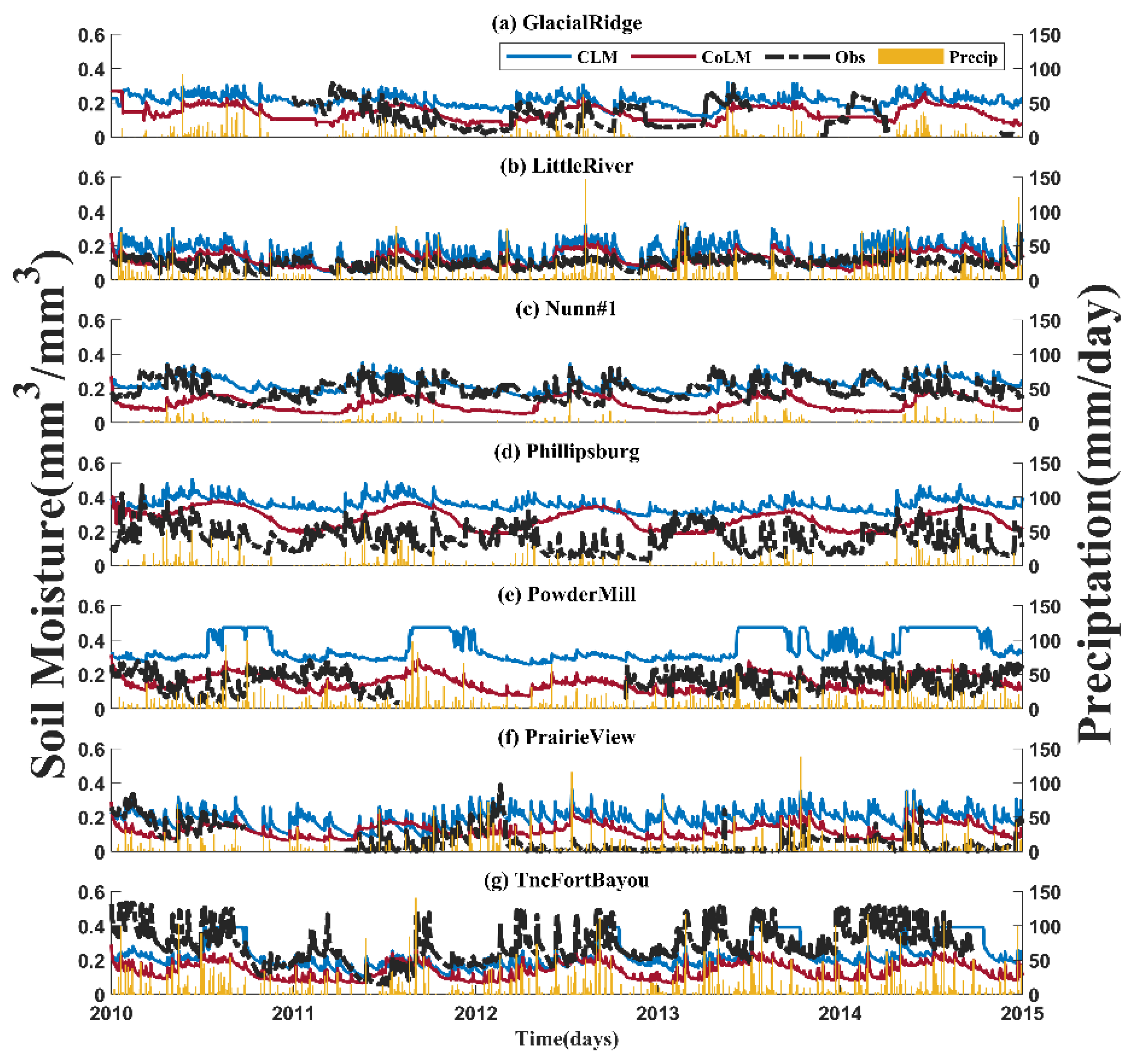
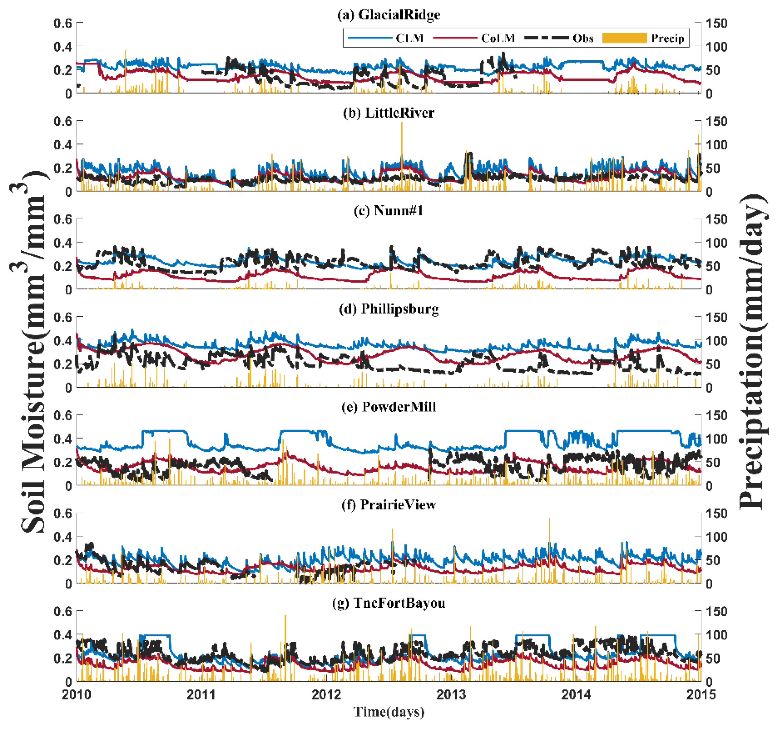
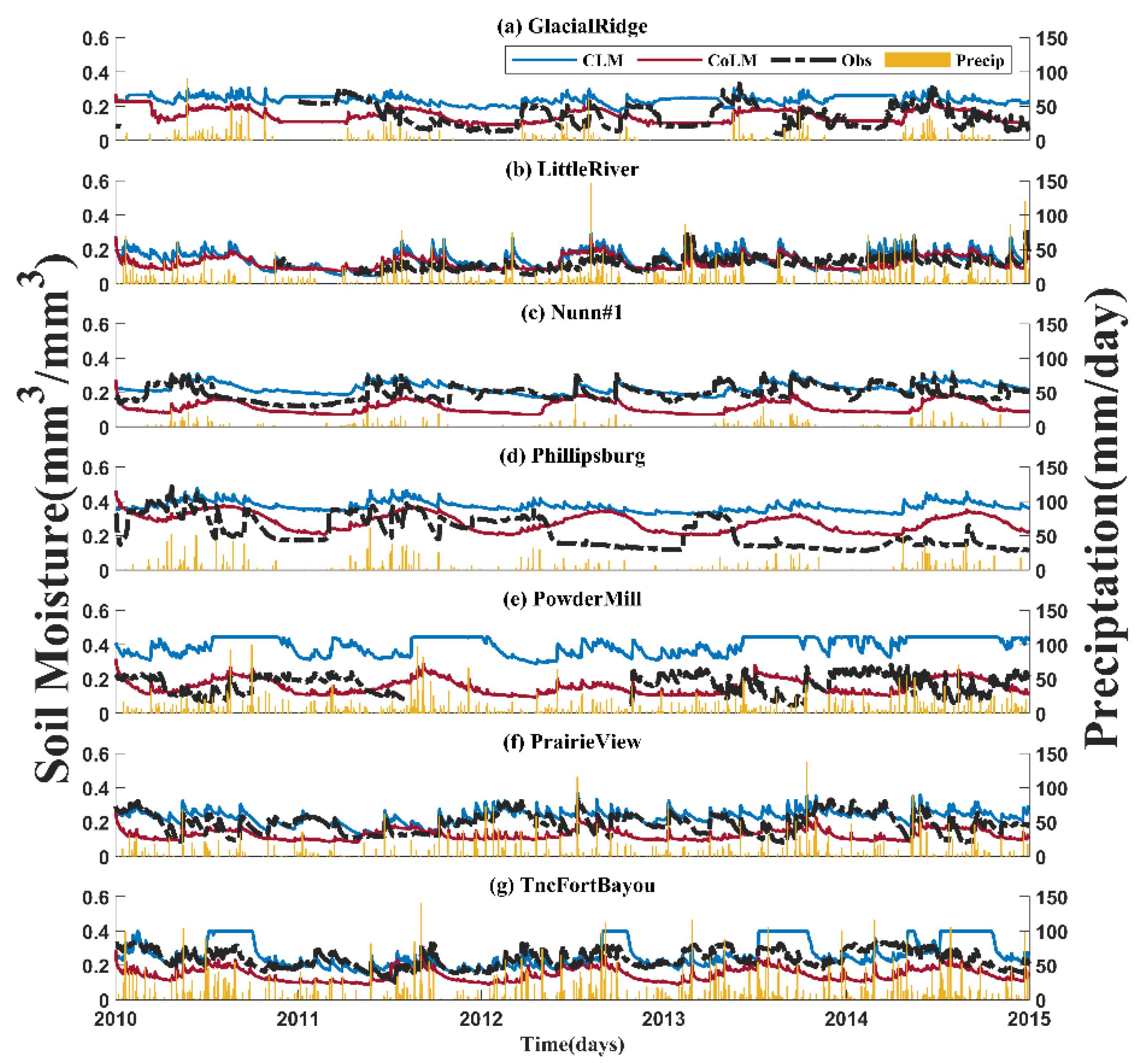
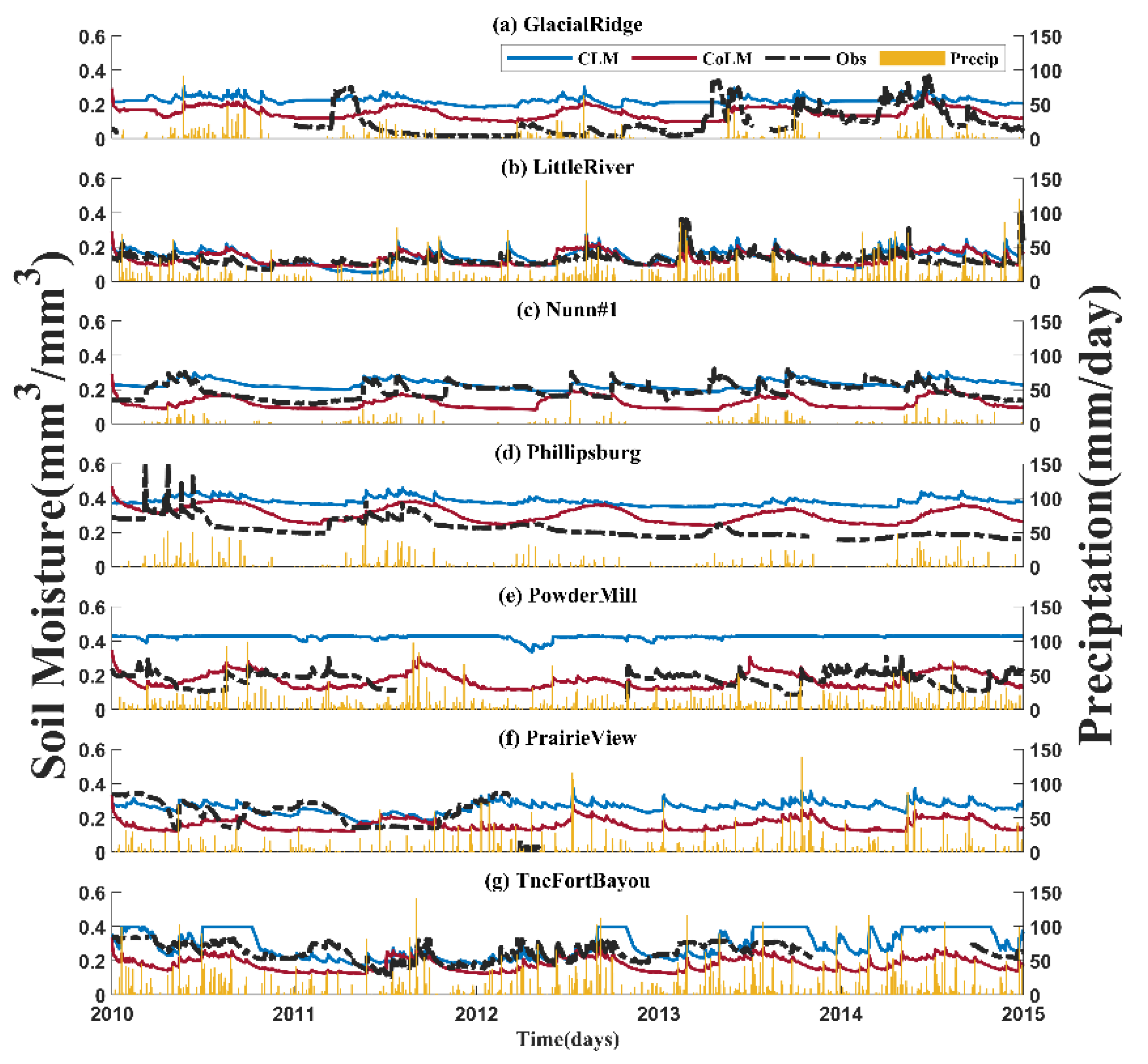
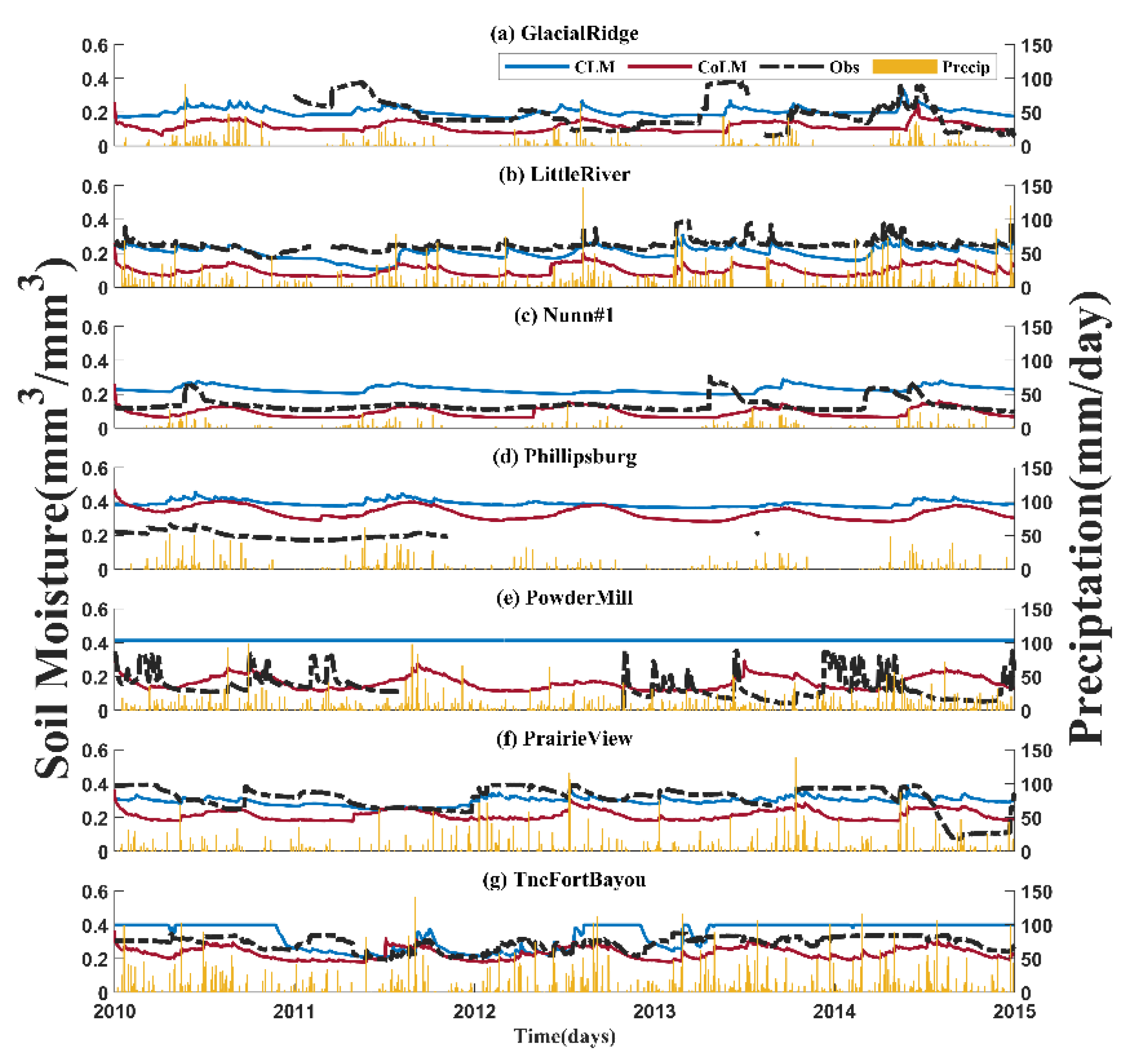
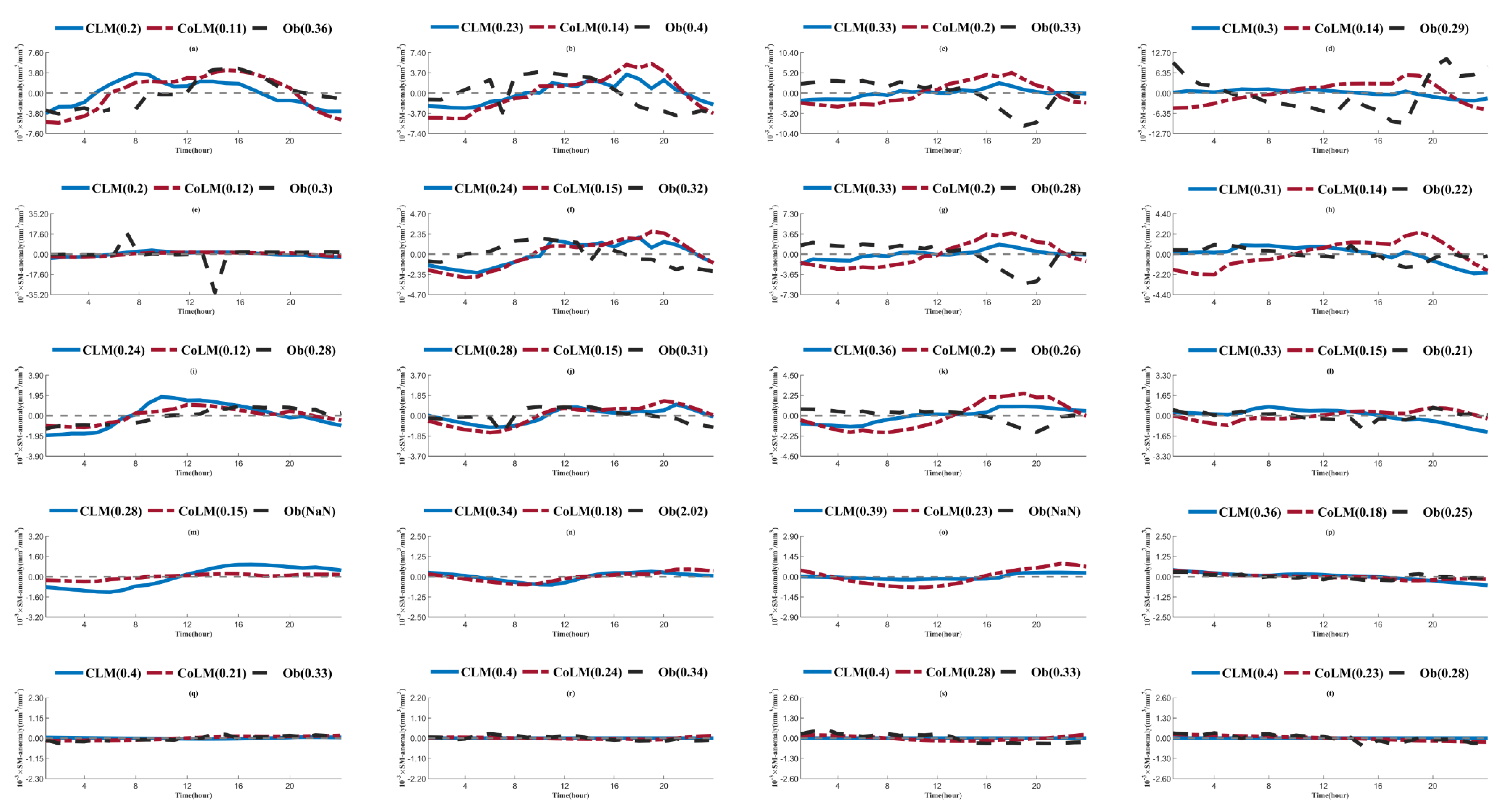
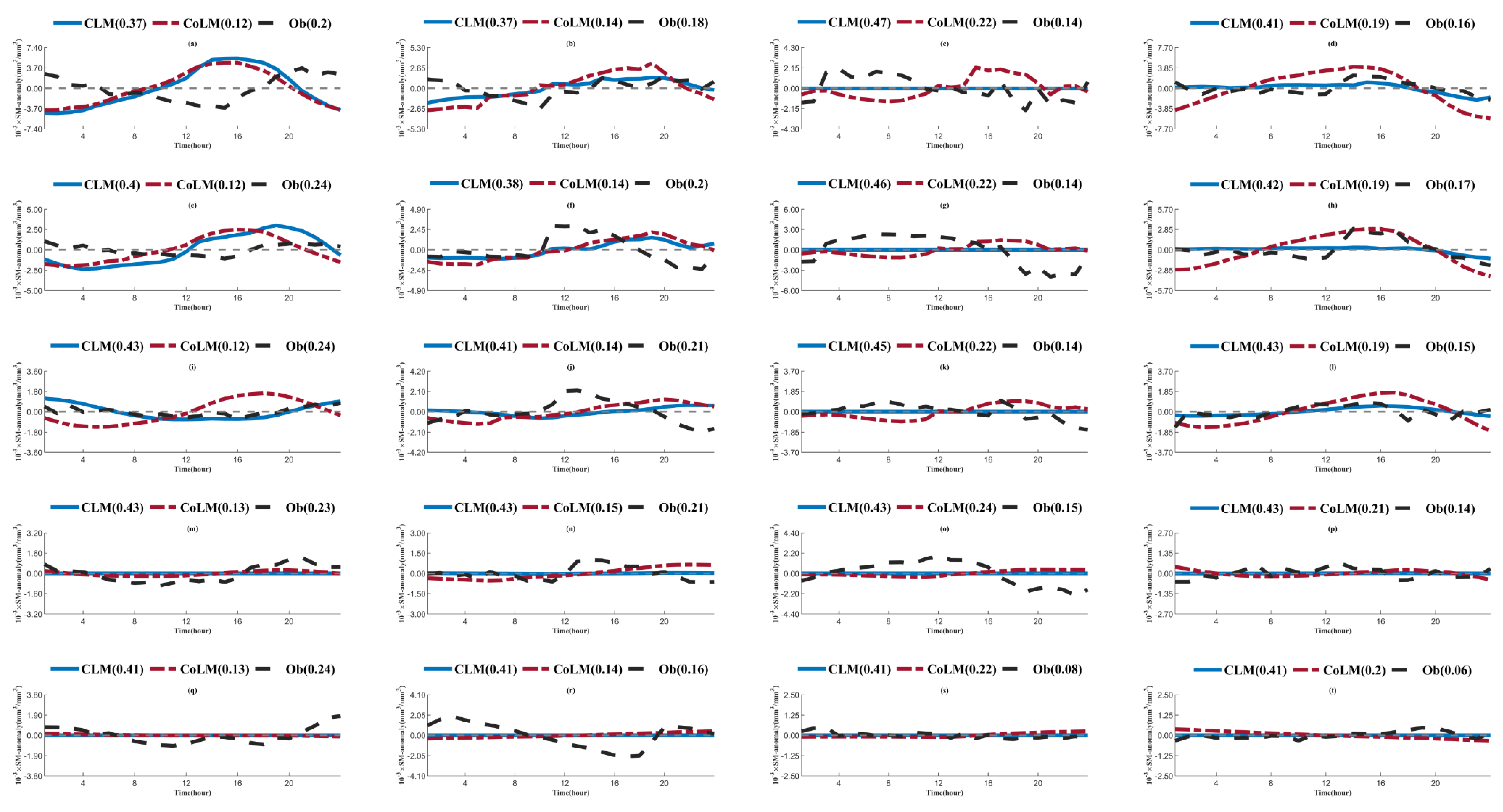
3.1. Soil Moisture Time Series Comparison

Figure 2, Figure 3, Figure 4, Figure 5 and Figure 6 show a comparison of the daily soil moisture observations and models’ soil moisture simulations at five soil depths (0.0508, 0.1016, 0.2032, 0.5080, and 1.016 m) from 2010 to 2014. Table 2 lists the correlation between the daily simulation results and the observed soil moisture at the seven sites.
In both CLM5 and CoLM2014, the correlation coefficient at the Little River station was the highest of all the considered stations. The land cover at Little River is grassland and the climate is temperate, with hot summers. The precipitation throughout the year is relatively uniform, and there is no freezing period. Therefore, in the shallow soil layers (0–0.1016 m), both models responded quickly to precipitation, demonstrating increased soil moisture. After precipitation, soil water infiltrates into deep soil layers and the shallow soil layer becomes drier, which is consistent with the observations (Figure 2, Figure 3, Figure 4, Figure 5 and Figure 6b). The maximum R in the CLM5 results (0.70) occurred in the first observation layer (0–0.0508 m). The physical processes affecting shallow soil water movement, such as rainfall and surface evaporation, are reasonably described by CLM5 at Little River, but the R decreased with increased soil depth. However, the R of the CoLM2014 results in the three shallow layers of observation (0–0.2032 m) varied little (0.40, 0.44, and 0.43), and R for the 0.2032–1.016 m layers decreased with increasing soil depth. Therefore, compared to observations, CLM5 and CoLM2014 at all observation depths (0–1.016 m) generally represented the interannual and annual variation in soil moisture. In terms of bias, the soil moisture simulated at the top four soil depths was overestimated by CoLM2014 and CLM5 (Table 3), but both models underestimated the soil moisture in the fifth soil layer. The RMSE values of the results by CoLM2014 are smaller than those of the CLM5 results (Table 4), indicating that soil moisture simulated by CoLM2014 was closer to the observations than that simulated by CLM5. CoLM2014 simulated lower soil moisture during almost all the simulation periods than CLM5. During summer, the response of the CoLM2014 simulation to precipitation was weaker than that of the CLM5 simulation in the shallow layer, although the CoLM2014 simulation values were still numerically larger than the observed values. During autumn and winter when precipitation was low, the CoLM2014 simulation of soil moisture was drier than the observation values.
The climate type and land cover at Prairie View station are the same as those at Little River, whereas Prairie View receives less daily precipitation than Little River throughout the year. The models’ simulated results significantly differed from the actual observations (Figure 2, Figure 3, Figure 4, Figure 5 and Figure 6f), particularly after persistent summer rainfall when the soil water flowed rapidly through the shallow soil layers and soil moisture increased. In terms of R, the CoLM2014 simulation agreed with the observations only in the second layer and weakly correlated with the observations in the other soil layers. The CLM5 simulation result agreed better with the observations in the top four layers (0.37, 0.48, 0.60, and 0.48) than that of CoLM2014 and had a slightly lower R in the fifth layer (0.27). The RMSE for the top layer indicated that both the CLM5 and CoLM2014 simulations significantly deviated from the observations. The maximum RMSE for CoLM2014 (0.1542   mm 3 · mm 3 ) occurred in the top layer. However, as the soil depth increased, the simulated values were gradually closer to the observations. The minimum RMSE in the CoLM2014 simulation (0.0631   mm 3 · mm 3 ) occurred in the second layer, and simulations deviated further from observations as soil depth increased. In terms of bias, the CLM5 simulation overestimated the observations in all the soil layers. The maximum bias (0.1369   mm 3 · mm 3 ) in the CLM5 simulations occurred in the top layer, and bias decreased as soil depth increased. The minimum bias in the CoLM2014 simulations ( 0.0182   mm 3 · mm 3 )  occurred in the second layer, and the simulations indicated drier conditions than the observed values as soil depth increased.
The climate type at Tnc Fort Bayou station is also the same as that at Little River station. The land cover is shrubby, and precipitation is frequent and heavy throughout the year. The rainy period in each year starts in January and ends in August. During the rainy season, the soil moisture in the top layer is mainly influenced by precipitation; the soil is wetter here than at the Little River and Prairie View stations. Generally, the CLM5 simulation correlated with the observations in all the soil layers. R increased with soil depth, with the maximum R (0.52) occurring in the fifth soil layer. The CoLM2014 simulation had a slightly lower R between the simulation and observed values than the CLM5 simulation in the top two layers. R decreased as soil depth increased, with the smallest value (0.28) occurring in the fifth layer. This indicated that the variation in soil moisture in the deeper soil layer was better simulated by CLM5 than by CoLM2014. Although CLM5 and CoLM2014 were able to simulate the variation in the soil moisture in the top layer, the largest RMSE between the simulation and observation occurred in this layer, at 0.1181 mm 3 · mm 3 for the CLM5 simulation and 0.1738   mm 3 · mm 3  for the CoLM2014 simulation. As the soil depth increased, the simulation value became closer to the observation. Due to the increased precipitation at this site compared to the other sites, both models underestimated the observations in the top soil layer (Figure 2c). As the soil depth increased (Figure 3, Figure 4, Figure 5 and Figure 6c), the CLM5 simulation increasingly overestimated the soil moisture, especially in July, during which the soil moisture reached saturation. The CoLM2014 simulation underestimated the soil moisture in all the layers, with negative deviations.
Powder Mill, Phillipsburg, and Nunn#1 stations are located at middle latitudes and are covered by grass, but their climate types differ by longitude (Table 1). Overall, the soil moisture variations simulated by CoLM2014 and CLM5 were generally consistent with the observations (Figure 2, Figure 3, Figure 4, Figure 5 and Figure 6). The CLM5 simulation had a stronger correlation (R) than CoLM2014 at two sites (Nunn#1 and Phillipsburg), which are located in semi-arid areas (Table 2). The CLM5 simulation at Phillipsburg performed the best among these three sites, with a mean R of 0.42. In terms of RMSE, both the CLM5 and CoLM2014 simulations were close to the observations (Table 3). The CLM5 simulation indicated wetter soil than was observed at all soil depths, whereas CoLM2014 simulated drier soil (Table 4). The bias of the CLM5 simulation was generally greater than that of the CoLM2014 simulation (Table 4). At Powder Mill, which receives more precipitation, neither model simulation was reasonably consistent with the observations, especially during precipitation processes when the soil in the top layer quickly reached saturation in the CLM5 simulation. The large bias at Powder Mill station may be related to its topography, which is ignored in the models.
Glacial Ridge station is located at a high latitude. The landcover type is cropland and the climate is boreal. The precipitation at this station is concentrated in summer but low. In terms of R, the CLM5 simulation was more consistent with the observed values than the CoLM2014 simulation, with the maximum R between the simulation and observation values for both models occurring in the third and fourth soil layer. The lowest R occurred in the second soil layer (Table 2). The soil moisture variations in the top three layers at Glacial Ridge are impacted mainly by precipitation, with a significant increase occurring in the top layer when rain falls on the surface. Moreover, since the second layer receives water infiltrated from the top layer, we noted that the variation in this layer was lower compared to that in the top layer. The same variation was found in the third layer (Figure 2, Figure 3 and Figure 4). In the deepest two layers, the main reason for the variation in the soil moisture was the infiltration of soil moisture from the upper layer to the lower layer (Figure 5 and Figure 6a). For CoLM2014 and CLM5, the soil moisture simulations for the top three layers were responsive to the precipitation on the surface, but, in terms of RMSE (Table 3), both the CoLM2014 and CLM5 simulated values deviated significantly from the observed values. In terms of bias, both models simulated wetter soil than was observed in the top four layers, and the bias of CLM5 was twice that of CoLM2014. In the deepest layer, the CLM5 simulation was closer to the observations and had a smaller bias than the CoLM2014 simulation.

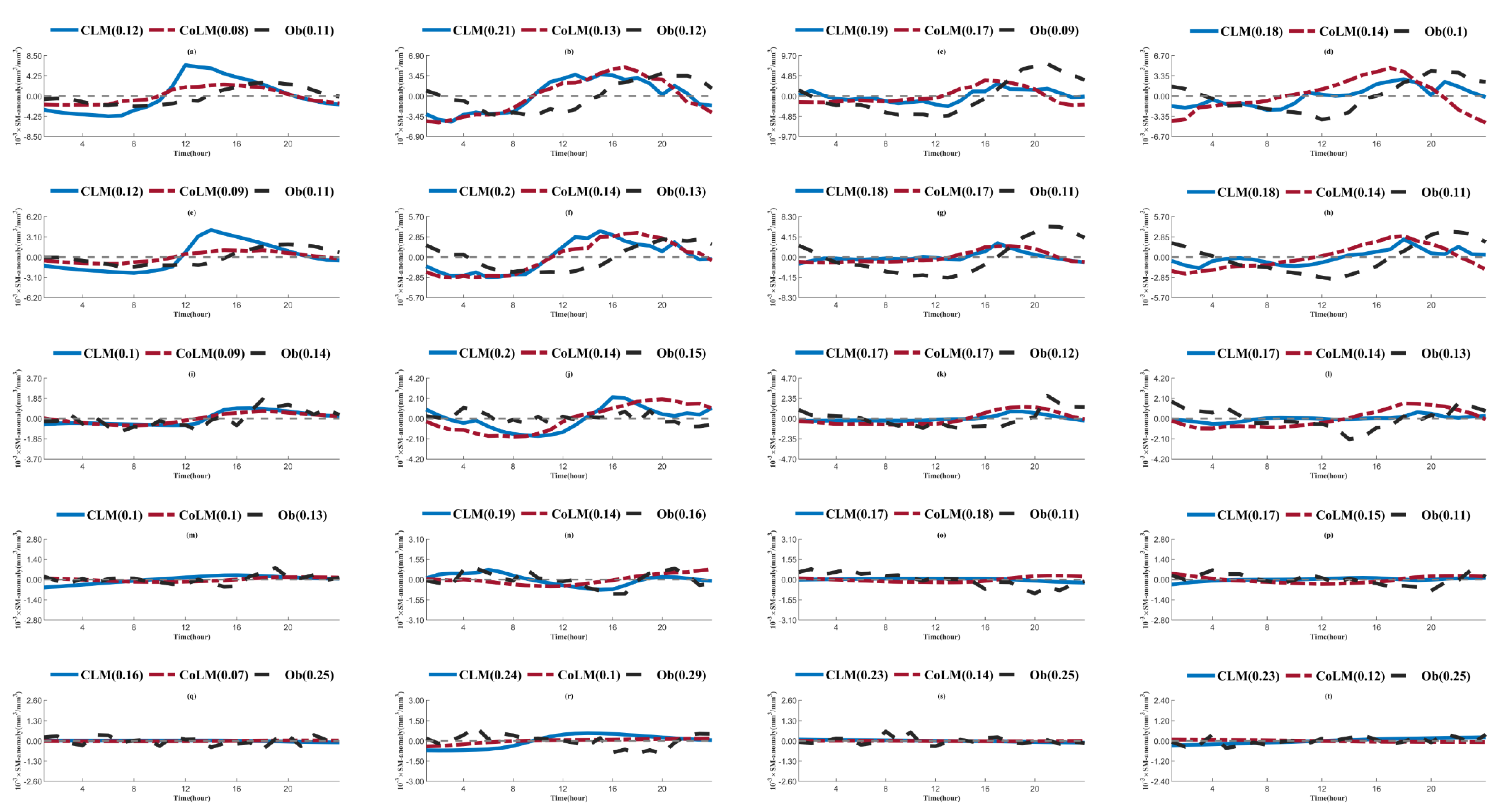
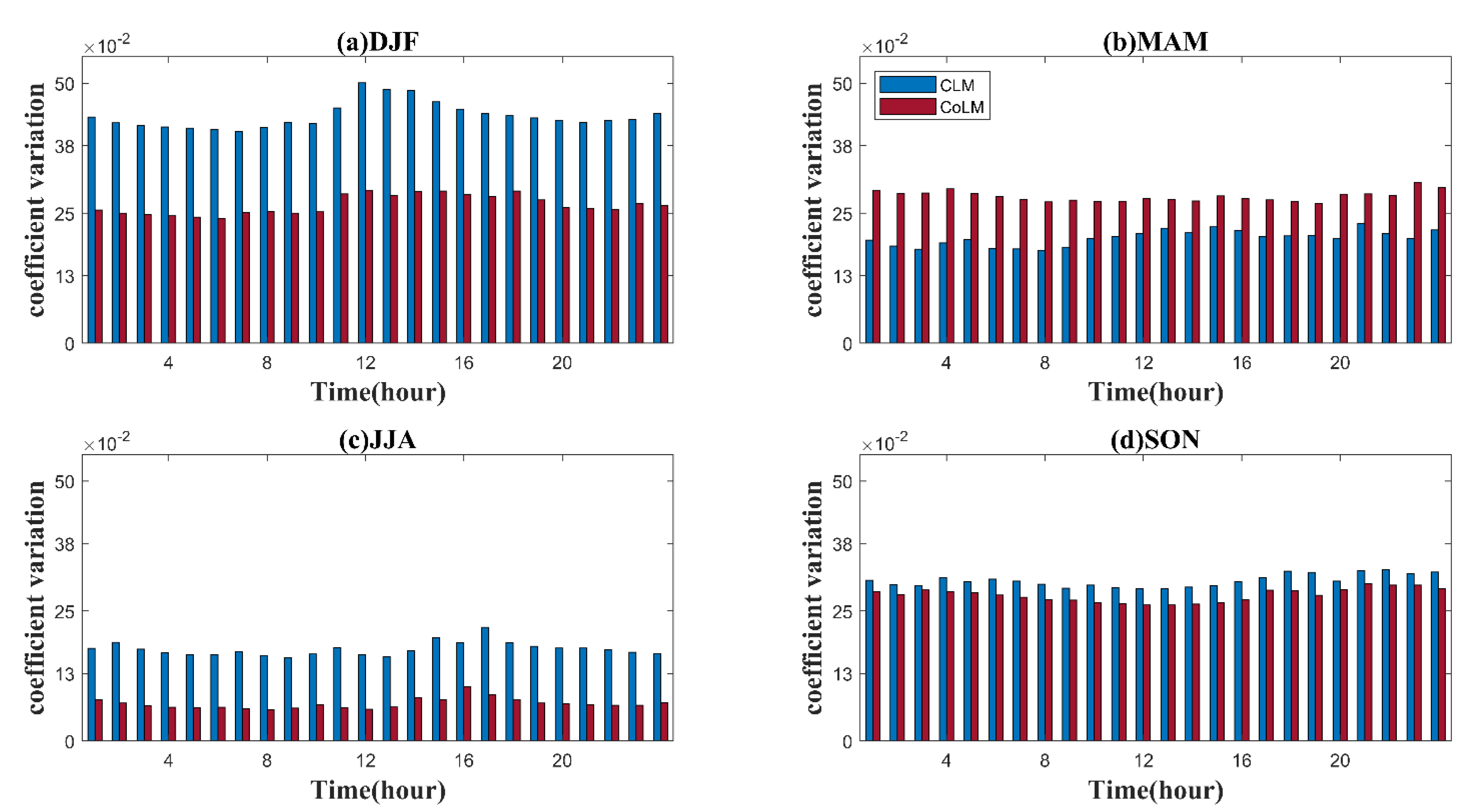
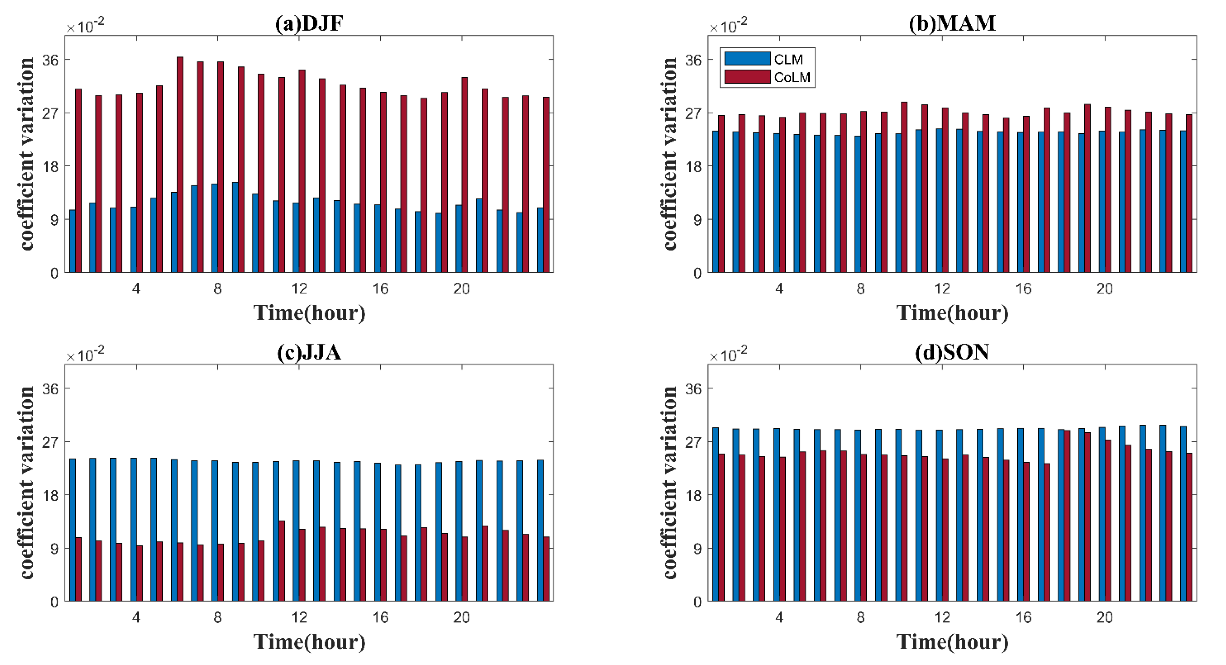
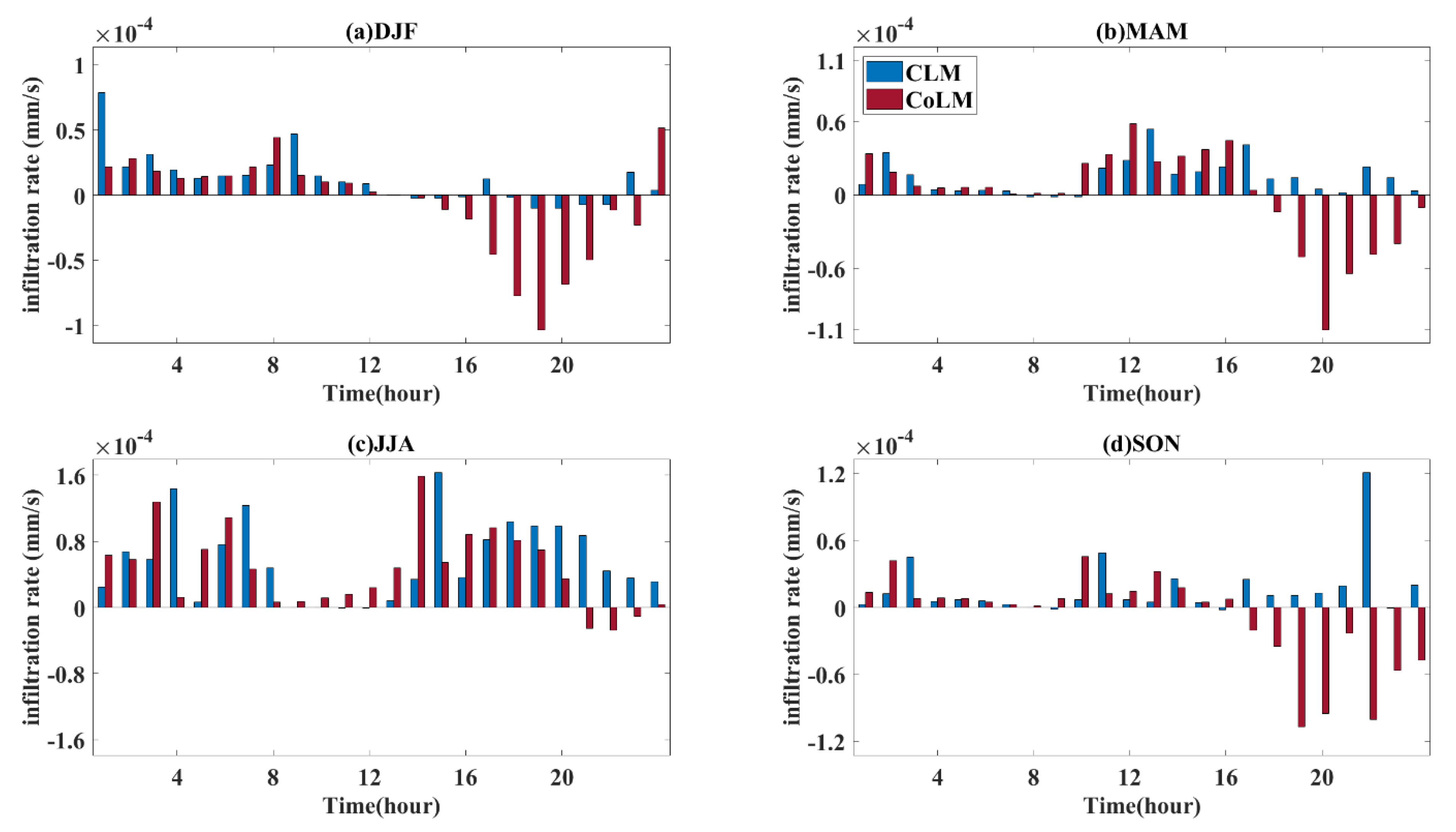
3.2. Soil Moisture Simulation Variance Analysis

Soil moisture is heterogeneous and is closely related to small-scale hydrological processes, soil properties, and land cover [7,33,34]. At the sites selected in this study, both models produced variations similar to the observations at most of the sites. In terms of R and RMSE, the CLM simulation’s performance at selected sites from highest to lowest was: Little River, Tnc Fort Bayou, Prairie View, Nunn#1, Glacial Ridge, Phillipsburg, and Powder Mill. The CoLM simulation’s performance from highest to lowest was: Little River, Tnc Fort Bayou, Prairie View, Glacial Ridge, Nunn #1, Phillipsburg, and Powder Mill. Considering the temporal completeness of the observation data, three sites, Little River, Tnc Fort Bayou, and Powder Mill, were selected to evaluate the simulated diurnal variations in soil moisture. Possible reasons for the differences in the model performances were analyzed.
Both CLM5 and CoLM2014 perform best at Little River station. The diurnal variations in soil moisture anomalies in four seasons at Little River station are shown in Figure 7, and their shallowest layer’s temporal stability of soil moisture values are shown in Figure 8 The seasonal variation in soil moisture is consistent with the interannual variation in soil moisture (Figure 2, Figure 3, Figure 4, Figure 5 and Figure 6b), with a reasonable match between the simulation and observation in all the soil layers at this site. The observed soil is wettest in spring (MAM) in the top layer, with a mean soil moisture of 0.1232   mm 3 · mm 3 . Both CLM5 and CoLM2014 simulated the most stable soil moisture (Figure 8c) in summer (JJA), and the most unstable soil moisture in winter (DJF) (Figure 8a). However, CoLM2014 simulated the soil moisture in the top layer as being highest in the summer (JJA), and the values were closer to the observations than those produced by the CLM5 simulation. CLM5 simulated the daily maximum in soil moisture earlier than the observations recorded in spring and winter. As the soil depth increased, the time when soil moisture simulation attained the maximum by CLM5 simulation became closer to the observed time. The time when CoLM2014 simulation in the top two layers reached the maximum was around 18:00 in all seasons, which is close to the observations. The bias of the CoLM2014 simulation is smaller than that of the CLM5 simulation, and the variation curve of the CoLM2014 simulation is more consistent with that of the observations.
Tnc Fort Bayou and Little River are similar in geographic location and climatic characteristics, except for land cover type (shrub and grassland, respectively). However, the hourly mean soil moisture differs considerably at the two sites. At Tnc Fort Bayou, the wettest soil was observed in the top layer in spring (MAM), with a value of 0.4052   mm 3 · mm 3 (Figure 9), which may relate to the high precipitation (Figure 2, Figure 3, Figure 4, Figure 5 and Figure 6g). In spring and winter, the variation curves of the CLM5 and CoLM2014 simulations agreed with the observations; additionally, the CoLM2014 simulation was less stable than the CLM5 in winter and spring (Figure 10a,b). The CLM5 simulation’s daily maximum value occurred earlier than that of the CoLM2014 simulation in winter. Both the CoLM2014 and CLM5 simulations reached their daily maximum soil moisture value at around 18:00 in spring, which is later than the observed time. The soil moisture simulated in summer significantly differed from the observation. In summer, both models stimulated that the soil in the top three layers became progressively wetter from 0:00 to 16:00 and then progressively drier from 16:00 to 24:00. In summer and autumn, rainfall events contributed to the increase in the C v ( θ ) , where the CLM5 simulation’s C v ( θ ) was higher than that of CoLM2014. This difference between the simulations and observations is probably due to hydrological processes ignored in models. In autumn, the observed soil was progressively drier during daytime and the rate of change decreased as soil depth increased. The CLM5-simulated variation was more consistent with the observations but disagreed with that simulated by CoLM2014. The CLM5 simulation captured the re-wetting processes in shallow soil layers between 16:00 and 20:00 in autumn. The CoLM2014 simulation was barely able to represent the diurnal variation in soil moisture in autumn.
At the Powder Mill site, both models produced less accurate results in the daily mean soil moisture than at the Little River and Tnc Fort Bayou sites (Table 2, Table 3 and Table 4). At Little River, with grassland as its land cover type, that soil has a high sand percentage and lower contents of other components, such as silt and clay, which leads to rapid drainage and poor water retention capability. By contrast, the predominant soil type at Tnc Fort Bayou and Powder Mill is well-drained and water-retentive sandy loam, with shrubs covering the ground surface at the Tnc Fort Bayou site and grass at the Powder Mill site. Precipitation at Powder Mill is concentrated in summer (Figure 2, Figure 3, Figure 4, Figure 5 and Figure 6e), whereas the observed soil is wettest in winter, with evenly distributed moisture across all depths (Figure 11). Except for summer, the CoLM2014-simulated diurnal variation was generally consistent with the CLM5 simulation in the top two layers (Figure 11). However, beginning with the third layer, CLM5 simulated almost saturated soil (Figure 11-blue line) and overestimated the soil moisture all year round. Therefore, the RMSE and bias were larger between the CLM5 simulation and the observations, whereas the CoLM2014 simulation only overestimated the soil moisture in summer and autumn. CoLM2014 simulated a drier soil than observed in winter and spring (Figure 11, red line) and had a smaller RMSE and bias than the CLM5 simulation. Since Powder Mill is a site with a moderate slope (4%), and both models lack soil water movement parameterization considering lateral flow in slope areas, they could not capture the characteristics of soil moisture variation. Compared to the CLM5 simulation, the CoLM2014-simulated soil moisture was numerically closer to the observations.
The differences in the soil moisture simulation capabilities of the two models are mainly due to the models’ numerical soil water movement schemes. The variations in hourly soil moisture in the shallow layers are influenced by the combination of soil texture and precipitation. In the land surface water balance equation, precipitation is divided into infiltration, plant canopy interception, and surface runoff. Infiltration is a crucial process for redistributing precipitation and is mainly influenced by the soil texture and the soil water content near surface. Soil texture determines the saturated hydraulic conductivity, saturated water content, and soil water potential. Little River and Tnc Fort Bayou are similar in latitude and climate type. However, the predominant soil type is sandy at Little River, whereas it is sandy loam at Tnc Fort Bayou; thus, the soil at the Little River site has higher hydraulic conductivity than that at Tnc Fort Bayou. Soil hydraulic properties could be well-represented by both models and impacted the calculations of infiltration rates. The simulated infiltration rate at Little River was generally lower than that at Tnc Fort Bayou throughout the year (Figure 12 and Figure 13). Due to the low water retention capability of sandy soil, the soil at Little River was drier than that at Tnc Fort Bayou. Soil moisture in shallow layers responds rapidly to the variations in infiltration rates. At Little River, both CLM5 and CoLM2014 simulated the maximum infiltration rate in the shallow layers in summer (Figure 12c), with differences in infiltration rates mainly occurring at times after 16:00. This is one of the reasons why CLM5 and CoLM2014 have similar simulation accuracies at Little River, but the CLM5 simulation overestimated the soil moisture more than the CoLM2014 simulation.
A key aspect of the parameterization scheme for the infiltration rates in the land surface model is the calculation of its maximum infiltration capacity q infl , max . In CLM5, q infl , max is calculated with hydraulic conductivity, which considers the ice impedance Θ ice  in the unsaturated regions [26],
q infl , max = ( 1 f sat ) · Θ ice · k sat ,
Θ ice = 10 6 · θ ice θ sat ,
However, in CoLM2014, an empirical formula is used to calculate the ice impedance Θ ice , and the maximum infiltration capacity is calculated as the minimum value of the infiltration rates in the top three layers:
q infl , max = min i = 1 , 2 , 3 { k sat , i 10 ( 6 · f ice , i ) } .
The calculations of q infl , max  affect the simulations of the runoff that is generated from excess infiltration and storage excess. Underestimation of infiltration rates reduces the water infiltrating into the soil’s top layers and further leads to a biased redistribution between terms in the surface energy balance. As shown in Figure 13, CoLM2014 simulated a generally lower infiltration rate than CLM5 at Tnc Fort Bayou. CoLM2014 simulated warmer soil temperatures during the same period than CLM5 (Figure 14b,c), especially during winter and spring when infiltration rates differ considerably. At Little River, CoLM2014 also simulated significantly warmer soil during spring and winter than CLM5 (Figure 15b,c). The overestimation of soil temperature increases the evaporation of shallow soil layers and results in drier soil.

4. Conclusions

The accuracy of soil moisture simulations primarily relies on the parameterization schemes and the precision of atmospheric forcing and surface data. In this study, we conducted offline land surface simulations at single points using CLM5 and CoLM2014, of which the atmospheric forcing and surface data were obtained from SCAN stations. The simulated soil moisture was interpolated to the soil depths of the observations to evaluate the performance accuracy of CLM5 and CoLM2014.
At the selected SCAN sites, the CLM5 simulations (0.38) had generally higher correlation coefficients than those of the CoLM2014 simulations (0.11). The correlation coefficients were highest at Little River, with mean values of 0.61 and 0.48 in all the soil layers for CLM5 and CoLM2014, respectively. The correlation coefficients were lowest at Powder Mill as the site has a moderate slope and the current lateral flow schemes in both models are insufficiently accurate. In terms of the correlation coefficient, the soil moisture variation simulated by CLM5 was closer to the observed soil moisture variation than that simulated by CoLM2014, especially in shallow soils (layers one to three) and during periods of intense precipitation.
In contrast to the correlation between the simulation and observations, the RMSEs of the CLM5 simulations were larger than those of the CoLM2014 simulations at almost all the sites, indicating that the CoLM2014 simulations were numerically closer to the observations than the CLM5 simulations. Both CoLM2014 and CLM5 performed best at Little River, with RMSE and bias decreasing with increasing soil depth. CLM5 performed the worst at Powder Mill, with an RMSE reaching 0.2458   mm 3 · mm 3 .
Both models’ simulations of the diurnal variation in soil moisture variation require improvement. The simulated diurnal variations in soil moisture corresponded reasonably to the observations only in the shallow soil layers (0–0.2032 m). Even at the site where the models were most accurate, Little River, in terms of seasonal infiltration rate, CLM5 simulated more soil moisture infiltration than CoLM2014 from the surface soil layer in winter and autumn, where the CoLM2014 infiltration rate was lower than that of CLM5: 295% and 255%, respectively. In summer, CoLM2014 simulated 23% more soil moisture infiltrating than CLM5 from the surface soil layer.
The differences in model performance occurred for multiple reasons. Although surface data, such as soil properties, vegetation function types, and land cover types, were obtained from observations at SCAN sites, the land surface models do not accurately describe physical processes, such as lateral flow processes. Additionally, soil moisture is observed at fixed depths, but it is nonlinear in space. The interpolation of soil moisture from model layers to observation depths is, therefore, inherently inaccurate.
Small-scale hydrology processes are not represented well in land surface models (LSMs), for example, lateral overland flow and subsurface flow, which may play a key role at hyper resolutions. In this study, CoLM2014 and CLM5 were evaluated on a few data-adequate sites in the North American region; we hope to evaluate and improve the LSMs using more observations. Continued research is needed to further evaluate the coefficient of variation in the land surface balance budget, which comprises precipitation, infiltration, soil water movement, evaporation, runoff, and subsurface runoff as these factors have been identified as key determinants of variability in soil moisture. We think evaluation results will provide assistance to model developers working on improving their land surface models; more accurate LSMs will benefit researchers working on climate change, natural disasters, etc.

Author Contributions

Conceptualization, M.O. and S.Z.; methodology, M.O. and S.Z.; investigation, M.O.; writing—original draft preparation, M.O.; writing—review and editing, S.Z.; visualization, M.O. All authors have read and agreed to the published version of the manuscript.

Funding

This research was supported by Natural Science Foundation of China (under grant 41730962 and 42075159), National Key R&D Program of China (grant no. 2017YFA0604300).

Data Availability Statement

The data presented in the study are available on request from the corresponding author.

Conflicts of Interest

The authors declare no conflict of interest.

References

  1. Walker, J.; Rowntree, P.R. The effect of soil moisture on circulation and rainfall in a tropical model. Q. J. R. Meteorol. Soc. 1977, 103, 29–46. [Google Scholar] [CrossRef]
  2. Rind, D. The Influence of Ground Moisture Conditions in North America on Summer Climate as Modeled in the GISS GCM. Mon. Weather. Rev. 1982, 110, 1487–1494. [Google Scholar] [CrossRef] [Green Version]
  3. Manabe, S. Climate and the ocean circulation: I. The atmospheric circulation and the hydrology of the earth’s surface. Mon. Weather. Rev. 1969, 97, 739–774. [Google Scholar] [CrossRef]
  4. Yeh, T.-C.; Wetherald, R.T.; Manabe, S. The Effect of Soil Moisture on the Short-Term Climate and Hydrology Change—A Numerical Experiment. Mon. Weather. Rev. 1984, 112, 474–490. [Google Scholar] [CrossRef] [Green Version]
  5. Fatichi, S.; Katul, G.G.; Ivanov, V.Y.; Pappas, C.; Paschalis, A.; Consolo, A.; Kim, J.; Burlando, P. Abiotic and biotic controls of soil moisture spatiotemporal variability and the occurrence of hysteresis. Water Resour. Res. 2015, 51, 3505–3524. [Google Scholar] [CrossRef]
  6. Srivastava, A.; Saco, P.M.; Rodriguez, J.F.; Kumari, N.; Chun, K.P.; Yetemen, O. The role of landscape morphology on soil moisture variability in semi-arid ecosystems. Hydrol. Processes 2020, 35, e13990. [Google Scholar] [CrossRef]
  7. Vinnikov, K.Y.; Robock, A.; Speranskaya, N.A.; Schlosser, C.A. Scales of temporal and spatial variability of midlatitude soil moisture. J. Geophys. Res. Atmos. 1996, 101, 7163–7174. [Google Scholar] [CrossRef]
  8. Dickinson, R.E. Global change and terrestrial hydrology—A review. Tellus A Dyn. Meteorol. Oceanogr. 1991, 43, 176–181. [Google Scholar] [CrossRef]
  9. Pitman, A.J. The evolution of, and revolution in, land surface schemes designed for climate models. R. Meteorol. Soc. 2003, 23, 479–510. [Google Scholar] [CrossRef]
  10. Sellers, P.; Dickinson, R.; Randall, D.; Betts, A.; Hall, F.; Berry, J.; Collatz, G.; Denning, A.; Mooney, H.; Nobre, C. Modeling the exchanges of energy, water, and carbon between continents and the atmosphere. Science 1997, 275, 502–509. [Google Scholar] [CrossRef] [Green Version]
  11. Oleson, K.; Lawrence, D.; Bonan, G.; Drewniak, B.; Huang, M.; Koven, C.; Levis, S.; Li, F.; Riley, W.; Subin, Z.; et al. Technical Description of Version 4.5 of the Community Land Model (CLM); National Center for Atmospheric Research (NCAR): Boulder, CO, USA, 2013. [Google Scholar]
  12. Bonan, G.B. Land Surface Model (LSM Version 1.0) for Ecological, Hydrological, and Atmospheric Studies: Technical Description and Users Guide; Technical note; National Center for Atmospheric Research: Boulder, CO, USA, 1996. [Google Scholar]
  13. Dickinson, E.; Henderson-Sellers, A.; Kennedy, J. Biosphere-Atmosphere Transfer Scheme (BATS) Version 1e as Coupled to the NCAR Community Climate Model; National Center for Atmospheric Research (NCAR): Boulder, CO, USA, 1993. [Google Scholar]
  14. Yongjiu, D.; Qingcun, Z. A land surface model (IAP94) for climate studies part I: Formulation and validation in off-line experiments. Adv. Atmos. Sci. 1997, 14, 433–460. [Google Scholar] [CrossRef]
  15. Dai, Y.; Zeng, X.; Dickinson, R.E.; Baker, I.; Bonan, G.B.; Bosilovich, M.G.; Denning, A.S.; Dirmeyer, P.A.; Houser, P.R.; Niu, G. The common land model. Am. Meteorol. Soc. 2003, 84, 1013–1024. [Google Scholar] [CrossRef] [Green Version]
  16. Xin, Y.; Bian, L.G.; Zhang, X.H. The application of CoLM to Arid region of Northwest China and Qinghai-Xizang Plateau. Plateau Meteorol. 2006, 25, 567–574. [Google Scholar]
  17. Ma, L.; Tang, L.; Li, Z. Simulation of land ETs of China with CoLM; SPIE: Bellingham, WA, USA, 2006; Volume 6200. [Google Scholar]
  18. Zheng, J.; Xie, Z.H.; Dai, Y.J.; Yuan, X.; Bi, X.Q. Coupling of the Common Land Model(CoLM) with the Regional Climate Model (RegCM3) and Its Preliminary Validation. Chin. J. Atmos. Sci. 2009, 33, 737–750. [Google Scholar] [CrossRef]
  19. Zeng, X.; Shaikh, M.; Dai, Y.; Dickinson, R.E.; Myneni, R. Coupling of the Common Land Model to the NCAR Community Climate Model. J. Clim. 2002, 15, 1832–1854. [Google Scholar] [CrossRef]
  20. Li, M.; Ma, Z.; Niu, G.-Y. Modeling spatial and temporal variations in soil moisture in China. Chin. Sci. Bull. 2011, 56, 1809–1820. [Google Scholar] [CrossRef] [Green Version]
  21. Zhu, C.; Shi, C.; Xi, L.; Huang, X. Simulation and Assessment of Soil Moisture at Different Depths in China Area. Meteorol. Sci. Technol. 2013, 41, 529–536. [Google Scholar]
  22. Yuan, Y.; Xin, L.A.I.; Yuanfa, G.; Jun, W.E.N.; Xu, D.; Lihua, Z.H.U.; Yongli, Z.; Bingyun, W.; Xin, W.; Zuoliang, W.; et al. CLM4.5 Model Simulation of Soil Moisture over the Qinghai-Xizang Plateau and Its Performance Evaluation. Chin. J. Atmos. Sci. 2019, 43, 676–690. [Google Scholar] [CrossRef]
  23. Li, C.; Lu, H.; Yang, K.; Wright, J.S.; Yu, L.; Chen, Y.; Huang, X.; Xu, S. Evaluation of the common land model (CoLM) from the perspective of water and energy budget simulation: Towards inclusion in CMIP6. Atmosphere 2017, 8, 141. [Google Scholar] [CrossRef] [Green Version]
  24. Western, A.W.; Grayson, R.B.; Blöschl, G.; Willgoose, G.R.; McMahon, T.A.J.W.r.r. Observed spatial organization of soil moisture and its relation to terrain indices. Water Resour. Res. 1999, 35, 797–810. [Google Scholar] [CrossRef] [Green Version]
  25. Wang, A.; Zeng, X.; Guo, D.J.J.o.H. Estimates of global surface hydrology and heat fluxes from the Community Land Model (CLM4. 5) with four atmospheric forcing datasets. J. Hydrometeorol. 2016, 17, 2493–2510. [Google Scholar] [CrossRef] [Green Version]
  26. Swenson, S.; Lawrence, D.; Lee, H. Improved simulation of the terrestrial hydrological cycle in permafrost regions by the Community Land Model. J. Adv. Modeling Earth Syst. 2012, 4, M08002. [Google Scholar] [CrossRef]
  27. Brunke, M.A.; Broxton, P.; Pelletier, J.; Gochis, D.; Hazenberg, P.; Lawrence, D.M.; Leung, L.R.; Niu, G.-Y.; Troch, P.A.; Zeng, X. Implementing and Evaluating Variable Soil Thickness in the Community Land Model, Version 4.5 (CLM4.5). J. Clim. 2016, 29, 3441–3461. [Google Scholar] [CrossRef]
  28. Clapp, R.B.; Hornberger, G.M. Empirical equations for some soil hydraulic properties. Water Resour. Res. 1978, 14, 601–604. [Google Scholar] [CrossRef] [Green Version]
  29. Shangguan, W.; Dai, Y.; Duan, Q.; Liu, B.; Yuan, H. A global soil data set for earth system modeling. J. Adv. Modeling Earth Syst. 2014, 6, 249–263. [Google Scholar] [CrossRef]
  30. Köppen, W. Das gepgraphisca System der Klimate. In Handbuch der Klimatologie; Köppen, W., Geiger, G., Eds.; Gebr. Borntraeger: Stuttgart, Germany, 1936; pp. 1–44. [Google Scholar]
  31. Anderson, J.R.; Hardy, E.E.; Roach, J.T.; Witmer, R.E. A Land Use and Land Cover Classification System for Use with Remote Sensor Data; Geological Survey Professional Paper 964; United States Department of the Interior: Washington, DC, USA, 1976. [Google Scholar]
  32. Cosby, B.; Hornberger, G.; Clapp, R.; Ginn, T. A statistical exploration of the relationships of soil moisture characteristics to the physical properties of soils. Water Resour. Res. 1984, 20, 682–690. [Google Scholar] [CrossRef] [Green Version]
  33. Crow, W.T.; Wood, E.F. Multi-scale dynamics of soil moisture variability observed during SGP’97. Geophys. Res. Lett. 1999, 26, 3485–3488. [Google Scholar] [CrossRef]
  34. Entin, J.K.; Robock, A.; Vinnikov, K.Y.; Hollinger, S.E.; Liu, S.; Namkhai, A. Temporal and spatial scales of observed soil moisture variations in the extratropics. J. Geophys. Res. Atmos. 2000, 105, 11865–11877. [Google Scholar] [CrossRef]
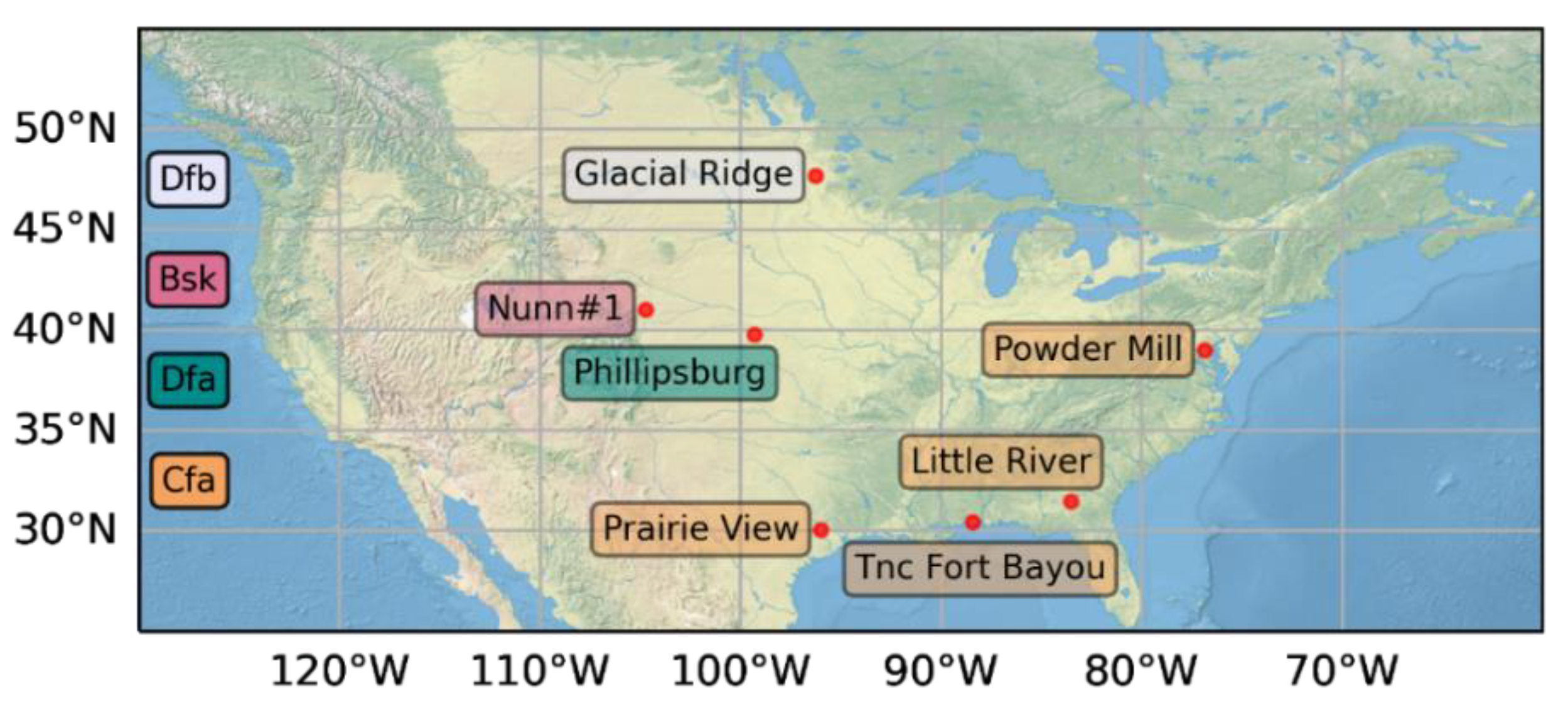
Figure 1. Overview of the selected SCAN sites’ locations. The color of the box represents the climate class.
Land 11 00126 g001
Figure 2. Simulation and observation temporal soil moisture variations at the SCAN sites for 2010–2014 at a soil depth of 0.0508 m. The blue line is the CLM5 simulation, the red line is the CoLM2014 simulation, the dashed line is the observations, and the yellow bars are the daily cumulative precipitation. (ag) are Glacial Ridge, Little River, Nunn#1, Phillipsburg, Powder Mill, Prairie View, and Tnc Fort Bayou, respectively.
Land 11 00126 g002
Figure 3. Simulated and observed temporal soil moisture variations at the SCAN sites for 2010–2014 at a soil depth of 0.1016 m. The blue line is the CLM5 simulation, the red line is the CoLM2014 simulation, the dashed line is the observations, and the yellow bars are the daily cumulative precipitation. (ag) Glacial Ridge, Little River, Nunn#1, Phillipsburg, Powder Mill, Prairie View, and Tnc Fort Bayou, respectively.
Land 11 00126 g003
Figure 4. Simulated and observed temporal soil moisture variations at the SCAN sites for 2010–2014 at a soil depth of 0.2032 m. The blue line is the CLM5 simulation, the red line is the CoLM2014 simulation, the dashed line is the observations, and the yellow bars are the daily cumulative precipitation. (ag) Glacial Ridge, Little River, Nunn#1, Phillipsburg, Powder Mill, Prairie View, and Tnc Fort Bayou, respectively.
Land 11 00126 g004
Figure 5. Simulated and observed temporal soil moisture variation values at the SCAN sites for 2010–2014 at a soil depth of 0.5080 m. The blue line is the CLM5 simulation, the red line is the CoLM2014 simulation, the dashed line is the observations, and the yellow bars are the daily cumulative precipitation. (ag) Glacial Ridge, Little River, Nunn#1, Phillipsburg, Powder Mill, Prairie View, and Tnc Fort Bayou, respectively.
Land 11 00126 g005
Figure 6. Simulated and observed temporal soil moisture variation at the SCAN sites for 2010–2014 at a soil depth of 1.0160 m. The blue line is the CLM5 simulation, the red line is the CoLM2014 simulation, the dashed line is the observation, and the yellow bars are the daily cumulative precipitation. (ag) Glacial Ridge, Little River, Nunn#1, Phillipsburg, Powder Mill, Prairie View, and Tnc Fort Bayou, respectively.
Land 11 00126 g006
Figure 7. Diurnal variations in soil moisture anomalies for the four seasons at the Little River site, with CLM5 in blue, CoLM2014 in red, and observations in black. The seasonal mean values of soil moisture are in brackets. Soil moisture anomalies in (a,e,i,m,q) winter in layers 1 to 5, respectively; (b,f,j,n,r) spring in layers 1 to 5, respectively; (c,g,k,o,s) summer in layers 1 to 5, respectively; and (d,h,l,p,t) autumn in layers 1 to 5, respectively.
Land 11 00126 g007
Figure 8. The shallowest layer’s coefficient of variation of diurnal simulations at the Little River site, with CLM5 simulations in blue bars and CoLM2014 simulations in red bars, for (ad) winter, spring, summer, and autumn, respectively.
Land 11 00126 g008
Figure 9. Anomalies in diurnal soil moisture variations in four seasons at Tnc Fort Bayou site, with CLM5 in blue, CoLM2014 in red, and observation in black. The seasonal mean values of soil moisture are in brackets. (a,e,i,m,q) Soil moisture anomalies in winter in layers 1 to 5, respectively. (b,f,j,n,r) Soil moisture anomalies in spring in layers 1 to 5, respectively. (c,g,k,o,s) Soil moisture anomalies in summer in layers 1 to 5, respectively. (d,h,l,p,t) Soil moisture anomalies in autumn in layers 1 to 5, respectively.
Land 11 00126 g009
Figure 10. The shallowest layer’s coefficient of variation of diurnal simulations at the Tnc Fort Bayou site, with CLM5 simulations in blue bars and CoLM2014 simulations in red bars, for (ad) winter, spring, summer, and autumn, respectively.
Land 11 00126 g010
Figure 11. Diurnal variations in soil moisture anomalies for the four seasons at Powder Mill, with CLM5 in blue, CoLM2014 in red, and observations in black. The seasonal mean values of soil moisture are in brackets. (a,e,i,m,q) Soil moisture anomalies in winter in layers 1 to 5, respectively. (b,f,j,n,r) Soil moisture anomalies in spring in layers 1 to 5, respectively. (c,g,k,o,s) Soil moisture anomalies in summer in layers 1 to 5, respectively. (d,h,l,p,t) Soil moisture anomalies in autumn in layers 1 to 5, respectively.
Land 11 00126 g011
Figure 12. Diurnal variation in the infiltration rate simulations at the Little River site, with CLM5 simulations in blue bars and CoLM2014 simulations in red bars, for (ad) for winter, spring, summer, and autumn, respectively.
Land 11 00126 g012
Figure 13. Diurnal variation in the infiltration rate simulations at the Tnc Fort Bayou site, with CLM5 simulations in blue bars and CoLM2014 simulations in red bars, for (ad) winter, spring, summer, and autumn, respectively.
Land 11 00126 g013
Figure 14. Soil temperature vertical profiles at Tnc Fort Bayou from 2010 to 2014: (a) observations, (b) the difference between CLM5’s simulation and the observations, and (c) difference between CoLM2014’s simulation and the observations.
Land 11 00126 g014
Figure 15. Soil temperature vertical profiles at Little River from 2010 to 2014: (a) is observations, (b) the difference between CLM5’s simulation and observations, and (c) the difference between CoLM2014’s simulation and observations.
Land 11 00126 g015
Table 1. Selected SCAN sites’ information and climatology. Climate class and climate group are defined according to Köppen climate classification [30]. Land cover types are defined by USGS classification [31].
IDSiteClimate ClassClimate GroupLatitudeLongitudePeriodLand-Cover Category (USGS)
1Glacial RidgeDfbTemperate continental with warm summers47°43′96°16′2010–2014Cropland
2Little RiverCfaSubtropical-Mediterranean39°47′99°20′2010–2014Grassland
3Nunn#1BskDry (arid and semi-arid)40°52′104°44′2010–2014Grassland
4PhillipsburgDfaTemperate continental with hot summers30°5′95°59′2010–2014Grassland
5Powder MillCfaSubtropical-Mediterranean30°28′88°28′2010–2014Grassland
6Prairie ViewCfaSubtropical-Mediterranean39°1′76°51′2010–2014Grassland
7Tnc Fort BayouCfaSubtropical-Mediterranean31°30′83°33′2010–2014Shrub
Table 2. Correlation coefficients between simulated and observed soil moisture at selected SCAN sites.
SiteModelSoil Depth
0.0508 m0.1016 m0.2032 m0.5080 m1.016 m
Glacial RidgeCLM50.24 0.17 0.40 0.50 0.27
CoLM20140.10 −0.10 0.16 0.16 −0.04
Little RiverCLM50.70 0.66 0.63 0.50 0.55
CoLM20140.40 0.44 0.43 0.34 0.36
Nunn#1CLM50.49 0.50 0.46 0.35 0.04
CoLM20140.00 0.03 0.10 0.06 0.11
PhillipsburgCLM50.32 0.41 0.40 0.55 0.42
CoLM2014−0.04 0.08 0.17 0.43 0.55
Powder MillCLM5−0.06 −0.07 −0.02 0.01 −0.01
CoLM2014−0.20 −0.35 −0.40 −0.42 −0.25
Prairie ViewCLM50.37 0.48 0.60 0.48 0.27
CoLM20140.06 0.27 −0.04 −0.26 −0.25
Tnc Fort BayouCLM50.44 0.44 0.43 0.45 0.52
CoLM20140.45 0.45 0.44 0.31 0.28
Table 3. Bias of simulated soil moisture at the selected SCAN sites.
SiteModelSoil Depth
0.0508 m0.1016 m0.2032 m0.0508 m1.016 m
Glacial RidgeCLM50.0749 0.1005 0.0924 0.1264 0.0126
CoLM2014−0.0003 0.0196 −0.0047 0.0519 −0.0757
Little RiverCLM50.0654 0.0547 0.0293 0.0183 −0.0419
CoLM20140.0244 0.0217 0.0083 0.0057 −0.1476
Nunn#1CLM50.0348 0.0112 0.0307 0.0386 0.0910
CoLM2014−0.0850 −0.1138 −0.0833 −0.0713 −0.0450
PhillipsburgCLM50.1963 0.1559 0.1521 0.1608 0.1969
CoLM20140.1119 0.0767 0.0602 0.0844 0.1533
Powder MillCLM50.2020 0.2091 0.2271 0.2487 0.2716
CoLM2014−0.0008 −0.0039 −0.0117 −0.0047 0.0230
Prairie ViewCLM50.1369 0.0557 0.0407 0.0192 −0.0127
CoLM20140.0602 −0.0182 −0.0655 −0.0728 −0.0970
Tnc Fort BayouCLM5−0.0577 −0.0018 0.0222 0.0273 0.0502
CoLM2014−0.1447 −0.0898 −0.0920 −0.0737 −0.0584
Table 4. RMSE of the simulated soil moisture at selected SCAN sites.
SiteModelSoil Depth
0.0508 m0.1016 m0.2032 m0.0508 m1.016 m
Glacial RidgeCLM50.1044 0.1264 0.1102 0.1471 0.0841
CoLM20140.0779 0.0911 0.0692 0.0992 0.1185
Little RiverCLM50.0782 0.0682 0.0488 0.0429 0.0534
CoLM20140.0462 0.0418 0.0394 0.0397 0.1519
Nunn#1CLM50.0612 0.0502 0.0511 0.0577 0.1004
CoLM20140.1090 0.1310 0.0988 0.0894 0.0634
PhillipsburgCLM50.2086 0.1665 0.1730 0.1666 0.1983
CoLM20140.1472 0.1112 0.1128 0.0990 0.1561
Powder MillCLM50.2256 0.2305 0.2386 0.2524 0.2817
CoLM20140.0834 0.0902 0.0837 0.0749 0.0966
Prairie ViewCLM50.1542 0.0794 0.0620 0.0728 0.0737
CoLM20140.1002 0.0631 0.0937 0.1169 0.1304
Tnc Fort BayouCLM50.1181 0.0793 0.0753 0.0825 0.0812
CoLM20140.1738 0.1082 0.1046 0.1005 0.0746
Publisher’s Note: MDPI stays neutral with regard to jurisdictional claims in published maps and institutional affiliations.

