Research on the Measurement Method of Benchmark Price of Rental Housing

Abstract

China’s rental housing market has just started to develop in recent years. It is relatively imperfect and lacks a clear reference for the pricing of rents, which is not fully transparent. A study on the rent formation mechanism of rental housing has policy implications for the construction of a guiding price for the rental housing market and the establishment of a reference basis for the pricing of subsidized housing. Referring to the definition of a benchmark land price, we use data from Beijing to innovatively introduce the concept of benchmark rent. Based on hedonic price theory and the driving factors of benchmark rent, a system of indicators is constructed to explore the mechanism of influencing factors at meso and micro levels on the benchmark rent of market-based rental housing. After LaGrange and robustness tests, it is found that the spatial error model (SEM) is more suitable for benchmark rent determination. We conclude that benchmark rents are affected by spatial relationships caused by spatial heterogeneity and dependency, and that there is significant spatial variation in the factors affecting market-based rental housing benchmark rents. The determination of the benchmark rent can be used as a guiding signal for the market, as a clear signal expectation for the market, government, and tenants.

1. Introduction

Due to the late development of China’s real estate market, coupled with the national policy orientation and the influence of residents’ cultural concepts, the housing rental market is hugely lagging [1] compared with the housing market. There are shortages of housing, insufficient coverage of affordable housing supply, and mismatches between market supply and demand [2,3,4]. Due to the lack of regulations related to rental housing, and the incomplete management system, there are still many hidden dangers in the operation of the rental housing market [5], which is not conducive to the formation of a stable rental relationship and market environment [4,6,7,8]; therefore, the increasing house-leasing market is significant in making up for the shortcomings of China’s real estate market, ensuring housing equity, and promoting healthy and intensive economic development [9,10,11].

However, due to the influence of various factors such as regional conditions, personal preferences, information asymmetry, and so on, the rental housing market is not a completely competitive market, and there is a certain degree of market failure; therefore, it is necessary for the government to intervene to a certain extent to ensure the smooth and efficient functioning of the market [12]. Since 2006, the issue of housing leasing has received continuous attention from the government [13]. The “China Eleventh Five-Year Plan” emphasizes the need to strengthen the regulation of the housing rental market and promote housing gradient consumption, whereas the “China Twelfth Five-Year Plan” proposes a supply system that combines rental housing with the purchase of commercial housing. The most recent “China Thirteenth Five-Year Plan” further proposes a housing system of “equal rights to purchase and rent”. In addition, China also pointed out the need to accelerate the establishment of a multi-subject construction and multi-channel housing system [14]. The intensive policy documents in recent years have revealed the state’s emphasis on the housing rental market. Under the policy environment of China’s multi-subject construction—renting and selling—the government has not yet implemented unified supervision of the rental housing market; therefore, we believe it is necessary to clarify the concept of benchmark rent as a clear signal of expectations from the market, the government, and tenants to ensure the stable development of the housing rental market and to consider the underlying social and environmental well-being dimensions, as well as the inequality and sustainability indicators that escape GDP accounting [15].

The regulation of prices through a benchmark index system can effectively guide the development of public policy, and has been much studied in the housing market [12,16]; however for large cities with a net inflow of population, rental housing plays a more crucial role in solving the housing problems of the migrant population [17]. In the rental market, the location and transport conditions attached to the housing are important factors that influence the decision, and housing that is easily accessible tends to have higher rent [18,19]. Neighborhood income levels also have a positive effect on rental housing rent, whereas a negative environment can significantly reduce housing rental prices, reflecting the influence of neighborhood characteristics on housing rents [20,21]. In addition, aspects such as the size of the housing stock, the year in which it was built, the design of the house, the floor on which it is located, the degree of decoration, and other infrastructural support are also related to the rent of rental housing [16,22,23]. Considering the transient nature of renter occupancy compared with homebuyers, research has also found that amenity packages have an important impact on rent. There are also additional factors attached by landlords that are likely to have a significant impact on housing rents [24,25,26].

In general, in past research, the factors affecting housing prices and rent can be divided into macro, meso, and micro factors on a locational scale. Macro influencing factors mainly affect the movement of the overall level of rental housing rent at the city level, and therefore, they influence the differences in rental housing rent levels between cities, such as national macro policies, city and regional policies, the city’s level of socio-economic development, demographic conditions, investment in urban infrastructure, and the overall locational characteristics of the city in the country. Meso-influencing factors are the main factors that affect the differences in rental housing rent levels between different locational conditions within a city, such as employment opportunities, locational conditions, and the availability of public service facilities. Micro-influencing factors are factors that affect the rental level of rental housing within a neighborhood, such as green ratio, plot ratio, neighborhood environment, age of construction, floor level of the house, orientation of the house, decoration condition, and so on. Compared with macro-influencing factors, meso-influencing factors and micro-influencing factors are more intuitive in their impact on rental housing rents, facilitating observation, discussion, and analysis within the city; therefore, meso and micro factors will be mainly considered in this work’s system of impact factor indicators.

For the research on the benchmark rent measurement method of market-based rental housing, this article attempts to construct an index system of factors affecting market-based rental housing. Based on the hedonic theory, the driving factors are analyzed to construct a system of factors affecting the benchmark rent of market-based rental housing at the meso level, which is then further subdivided into four factor layers and eleven factor layers of neighborhood attributes, location characteristics, public services, and school district characteristics using the characteristic price theory. After the analysis, using the least squares (OLS) model, the spatial regression model was further applied to consider the spatial influence relationship. After the least squares (OLS) model analysis, further spatial regression modeling is applied to analyze the degree of influence and spatial dependency of the influencing factors and to construct a reasonable pricing method and model. The model is then used to analyze the degree of influence and spatial dependence of the influencing factors and to construct a reasonable pricing method and model.

2. Materials and Methods

2.1. Data Source

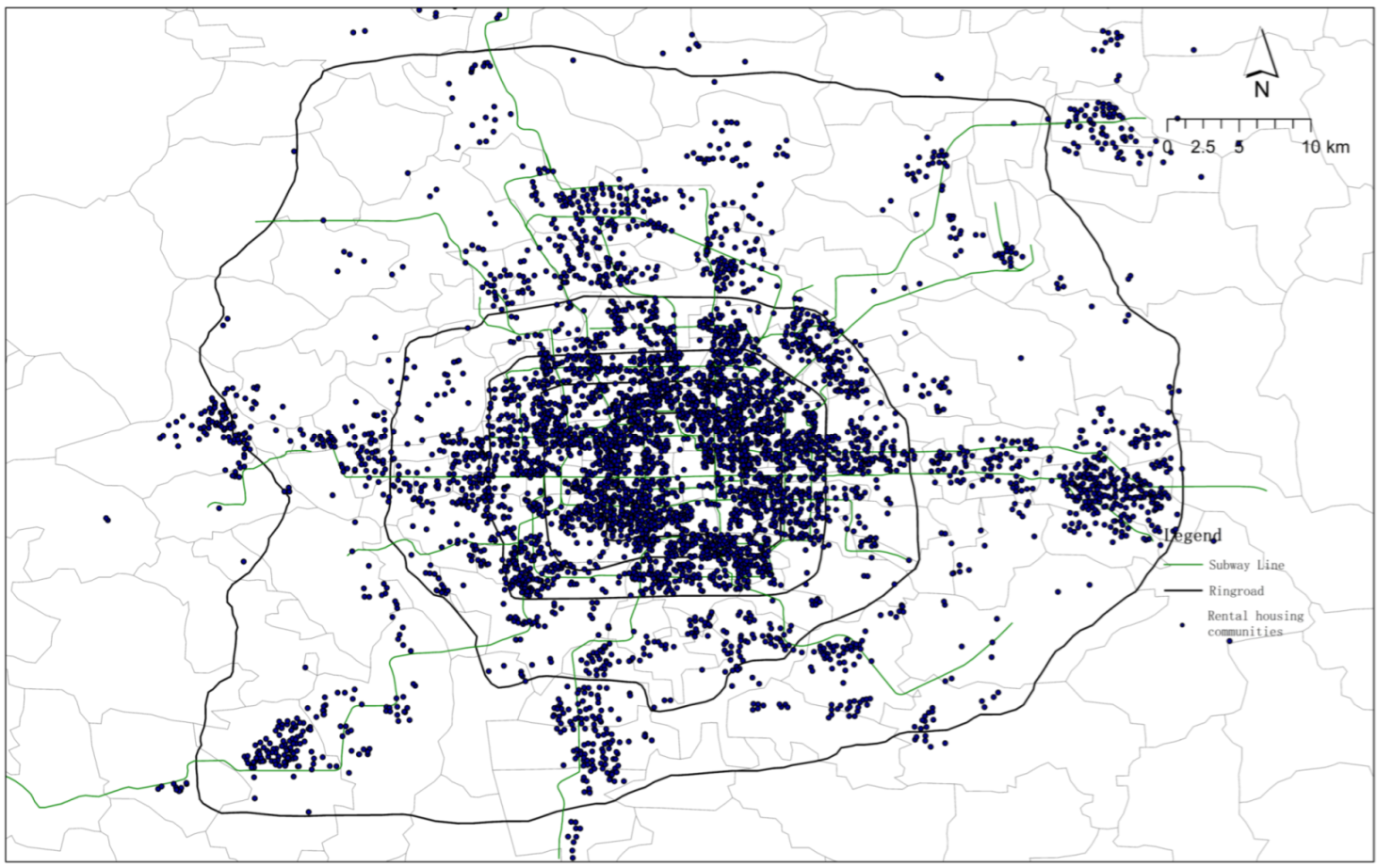
The rental transaction data of market-based rental housing in Beijing in 2018 came from the brokers’ listings on the website Lianjia.com. A total of 244,050 pieces of rental information were collected, covering 5980 communities (Figure 1). Since the number of houses released by the rental information of each community is quite different, to fully reflect the rental level of the community to a greater extent, in the process of data collection, we tried to ensure that the number of houses in each community were roughly equal. Except for the number of rental listings for individual communities less than 5, the number of rental collections in each community should be controlled as far as possible to 5–10 houses.

Borrowing the concept of benchmark land prices [27], this article defines benchmark rents as it is defined in the urban planning area, under the set community conditions, location conditions, and supporting facilities, for residential communities with different average values under the current utilization conditions and current development conditions [28]. The regional average rent of housing lease rights at a specific valuation date, in this study, refers to the average benchmark rent of each community and the rent level of specific houses. There are different types of average rent, based on decoration, floor, and house orientation. The main research subject of this article is the benchmark rent for rental housing. The calculation method of the benchmark rent of the community is the average of the unit rent of the residential housing (monthly rent price yuan/m²), not the total monthly rent of the housing divided by the total area.

It can be seen from Figure 1 that the market-based rental housing is relatively concentrated in the main urban area, and the periphery is extended along the subway line. The supply and demand of market-based rental housing reflect a complete market behavior [5,17]. The hypothesis of marketers, for the pricing model of market-based rental housing, allows us to apply a characteristic price model and a fixed rent factor.

To better reflect the spatial distribution of rents, when measuring the spatial difference of rent prices, this article uses community as the research unit instead of specific housing as the research unit; therefore, the dependent variable of the rent is the residential communities’ rent price, not the rental price of the listing.

2.2. Variables and Methods

Due to the complicated formation mechanism of urban housing prices, various factors comprehensively drive its spatial differentiation [29]. There is no consistent conclusion on the driving force that affects urban residential rental prices. The supply and demand theory [30] and the characteristic price theory [31] construct an index system of influencing factors from different perspectives. From the perspective of equilibrium price with demand, the characteristic price theory emphasizes that housing price is the monetary performance of urban environmental quality [32].

2.2.1. Benchmark Rent Driving Factors

• Urban planning:

The driving force of urban planning on housing rent is mainly manifested in the following three aspects: (1) Urban planning determines the nature of urban land use, land use function layout, development intensity, and other construction control requirements. Even if the land is of the same nature, different plots have different floor area ratios and building height limits. The economic benefits generated after the development of the plots are also significantly different, leading to an increase in housing rent difference. (2) Urban planning guides the construction and development of new urban areas (or sub-centers). With the increasing severity of urban diseases such as traffic congestion, excessive population density, and air pollution under the urban single-center structure, it is imperative to build and cultivate urban sub-centers or new urban districts, which requires scientific and reasonable urban planning. (3) To determine the new urban area (or sub-center) location problem. Take Beijing as an example [33]; as a suburb of Beijing, in the traditional sense, the rent in Tongzhou is far inferior to those of the six districts, however, after Tongzhou was officially planned as a sub-center in 2015, housing rent in this district has clearly shown a trend of substantial increase.

2.

Spatial differences in public goods investment:

Public goods investment includes public goods such as urban rail transit, education, medical care, and green spaces. The spatial difference in public goods investment directly reflects the spatial difference in the convenience and accessibility of public resources and has an essential impact on housing rents. Based on the finiteness of public resources, the difference in the scale, quality, and spatial distribution of public goods resources in different locations make the convenience of life in different communities in Beijing significantly different, leading to the spatial differentiation of housing rents. For example, rail transit will significantly affect the rent of leased housing along the line, and the benchmark rent level will also increase in areas with good infrastructure. Although large-scale communities such as Beijing Huilongguan and Tiantongyuan have a large population and robust rental demand, their rent levels are not high. The reason is that the surrounding supporting public service facilities are insufficient, making it difficult to support higher rents. People with a strong rent payment ability will prefer areas with better urban public goods.

3.

Transfer of urban residential land:

The transfer of urban residential land directly affects the location and traffic characteristics of residential quarters. Due to geographical restrictions, residential land available for sale in Beijing will become increasingly scarce in the future [20,25]. No matter what type of residential land, it will be favored by developers. With the increase in land acquisition costs caused by the shortage of land, developers often build high-end residential quarters on the land to obtain market benefits, thereby raising the level of housing rents in the area.

4.

Impact of the urban migrant population:

The first problem facing the migrant population in cities is the housing problem [23]. Due to household registration restrictions and payment constraints, rental housing is their first choice, and they directly reflect the needs of the residential rental market. Among them, migrant workers in Beijing and newly graduated students are the main support groups in the rental housing market in Beijing. Excessive growth of the migrant population has become a problem that must be addressed in the rapid development of Beijing. Although the government has introduced many restrictive policies, Beijing still has many migrant influxes every year, causing its housing rental demand to continuously rise, which can be seen from the housing occupancy rate of each district. In 2016, the average housing occupancy rate of various districts in Beijing was as high as 61% [22]. Moreover, the behavioral characteristics of the migrant population directly affect the rental prices in the rental market. For example, the return home season after the Spring Festival and the job-seeking rental season for college students from June to September each year are the peak demand seasons in the rental market, and rental prices often rise.

5.

Urban employment function orientation:

The “Beijing City Master Plan (2004–2020)” defines the two-axis, two-belt, and multi-center spatial development pattern of Beijing, and it is committed to building six industrial functional areas. With the government’s support for the construction of infrastructure in multi-center and industrial functional zones, the agglomeration effect of the parks is getting increasingly stronger, the number of jobs continues to increase, and a large amount of capital, funds, and labor are rapidly agglomerated, causing the housing rents in these areas to also increase. Beijing’s rent and high-value areas mostly overlap with the multi-center and six industrial functional areas defined in Beijing’s master plan, such as the China World Trade Center, Financial Street, Zhongguancun, and Wangjing.

2.2.2. Influencing Factor Index System

The benchmark rent of market-based rental housing is affected by the abovementioned multiple driving factors. The specific performance of these driving factors can be constructed from the four aspects of location transportation, employment accessibility, public services, and community attributes. In addition, rent may also be affected by housing facilities and lease methods. Due to the different housing types, areas, decoration standards, orientation, house facilities, and rental payment methods differ in each community, and thus the variability and randomness in individual housing are relatively large in order to better reflect the rent in a particular space. When measuring the spatial difference of rental prices, this paper uses the benchmark rent of the community as the research unit, rather than the specific housing rent as the research unit; therefore, the dependent variable of the benchmark rent is the residential benchmark rent, not the specific housing source rent. According to the results of literature research by scholars at home and abroad, we can define a four-factor, eleven-factor index system, and descriptive statistics of meso-level variables affecting rent prices as shown in

Table 1. Statistics for Variable Descriptions.

Variable Category	Explanatory Variable	Variable Description	Mean	STd	Expected (+/−)
Dependent variable	R	Average rental price per square meter of the community (yuan/m2)	31.62	10.07
Community attributes	Age	Year the community was built	11.08	3.16	−
	FAR	The ratio of the total construction area of the community to the land area	2.13	0.51	−
	Greening	Green coverage of the community (%)	0.31	0.03	+
Employment accessibility	D-job	Distance to the nearest employment center (m)	12,260.47	11,006.81	−
	C-job	Employment opportunities that can be reached within 60 min using public transportation	83.19	123.19	+
Location traffic	Bus	Number of bus stops within a radius of 1 km	415.78	367.87	+
	Subway	Number of subway stations within 1 km radius	2075.69	2177.47	+
Public Service	Park	Distance to the nearest park (m)	1701.08	1179.41	−
	Hospital	Distance to the nearest third-class hospital (m)	5688.15	5245.38	−
	Services	Number of large shopping malls and various supermarkets within 1 km radius	32.7627	27.18	+
	Preschool	Distance to the nearest key elementary school (m)	10,059.38	11,791.42	−

.

In the above variable indicator system, among the community attribute factors of the rental housing itself, the variables select three indicators: construction age, volume ratio, and greening rate. In terms of employment accessibility, to calculate the actual road network distance from one employment center to another employment center, a total of 15 employment centers were identified based on the characteristics of employment density [28]. From the center to the periphery are the Zhongguancun Center, Financial Street Center, CBD Center, Wangjing-Sun Palace Center, Yangfangdian Street Center, Shuguang Street Center, Datun Center, Jiuxianqiao Center, Shangdi Center, Capital Airport Center, Ten Balidian Center, Ancient City Center, Xincun Center, Yizhuang Center, and Baishan Center.

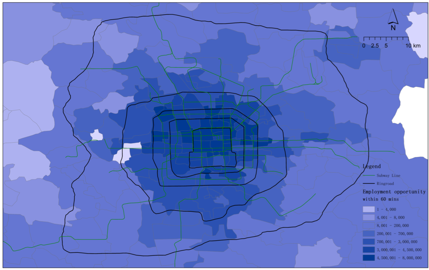
The employment opportunity data comes from the Beijing Employment Accessibility Map [33], which depicts the total number of employment opportunities that people who use the city’s public transportation system can achieve in 30, 45, and 60 min travel times across streets, towns, and villages in Beijing’s metropolitan area.

This article selects the employment opportunities that can be achieved within 60 min using public transportation. Figure 2 identifies the total number of employment centers in the area that are reached within 60 min (based on the morning rush hour) from the center of each street. The darker the color, the more employment opportunities. The distance from the nearest bus station and subway station to the nearest bus station and the subway station is selected at the level of location and traffic factors. At the same time, in order to make the calculation result closer to the reality of life, the measured distance we use here is the actual road network distance to represent its traffic convenience rather than straight-line distance. For the public service factor level, we chose the distance to the nearest parks, third-class hospitals, and key primary schools. The number of large shopping malls and various supermarkets within 1 km represents the degree of public goods investment. The data for various elementary schools comes from the Beijing “kindergarten to primary school “website (http://www.ysxiao.cn/ (accessed on 31 May 2018)), and measuring other variables (such as the distance to the nearest park, third-class hospitals) is also the actual road network calculated by the near tool distance. The quantity measurement of various variables (such as the number of shopping malls and supermarkets) within 1 km is realized by buffer analysis in Arcgis, which is also the distance of the road network. References to each data source and year are shown in

Table 2. Source for the Statistics of the Variables.

Variable Category	Explanatory Variable	Source of Variable	Reference of Year
Dependent variable	R (Benchmark rent)	/
Community attributes	Age (Year of construction)	Data from Lianjia website (https://bj.lianjia.com/ (accessed on 1 October 2018))	2018
	FAR (Floor Area Ratio)	Data from Lianjia website (https://bj.lianjia.com/ (accessed on 1 October 2018))	2018
	Greening (Greening ratio)	Data from Lianjia website (https://bj.lianjia.com/ (accessed on 1 October 2018))	2018
Employment accessibility	D-job (Distance to the Job Centre)	Calculated from Beijing Employment Centre Distribution [28]	2016
	C-job (Number of job opportunities)	Calculated from Beijing Job Accessibility Map [34]	2015
Location traffic	Bus (Bus stations within 1 km)	POI data extracted from Baidu Maps (https://map.baidu.com/ (accessed on 31 May 2018))	2018
	Subway (Subway stations within 1 km)	POI data extracted from Baidu Maps (https://map.baidu.com/ (accessed on 31 May 2018))	2018
Public Service	Park (Distance to the nearest park)	POI data extracted from Baidu Maps (https://map.baidu.com/ (accessed on 31 May 2018))	2018
	Hospital (Distance to the nearest third-class hospital)	POI data extracted from Baidu Maps (https://map.baidu.com/ (accessed on 31 May 2018))	2018
	Service (Malls/supermarkets within 1 km)	POI data extracted from Baidu Maps (https://map.baidu.com/ (accessed on 31 May 2018))	2018
	Preschool (Distance to the nearest key elementary school)	Calculated from Beijing “kindergarten to primary school” website (http://www.ysxiao.cn/ (accessed on 31 May 2018))	2018

.

2.2.3. Methods

Set the latitude and longitude coordinates with the help of Google Maps, import ArcGIS to establish the corresponding point layer, and match the latest Beijing GIS electronic base map to establish a rental housing sample database. Among them, the spatial data includes the latitude and longitude coordinates (X, Y) of the sample rental housing community, the street information of the rental housing, and the supporting public service facilities, such as subway stations, bus stations, parks, and green spaces, top three hospitals, key primary schools, and shopping malls. Attribute data includes transaction time, rental price, living area, construction age, volume ratio, and the sample rental housing communities’ greening rate.

Existing studies usually use OLS estimation and extended forms of characteristic price functions (semi-log model and double log model) to estimate the correlation coefficient of explanatory variables. In the characteristic price model, explanatory variables such as location characteristics and public services usually show spatial similarity or spatial dependence, and prices are also affected by unobservable latent variables. When omitted variables and spatial dependence coexist, OLS estimation will make the biased fluctuations have poor inference results, and the spatial measurement model can be used to analyze spatial dependence and spatial heterogeneity and avoid least squares estimation. This is problem of bias.

When choosing a spatial regression model, the specific model setting form must be considered, along with the mutual influence between independent variables and dependent variables. The spatial autoregressive model (SAR) considers the spatial dependence characteristics between the samples of the dependent variable; this model is used based on the belief that the dependent variable will have a certain external effect on the dependent variable of other spatial sample units. For a spatial unit $A_i$ (i = 1, 2, ..., n), regarding the observations of its neighborhood $A_j\left(i\ne j\right)$, the expression of the spatial autoregressive model (SAR) model is:

$${\mathrm{y}}_i=\mathsf{\rho }{\displaystyle \sum }_{j=1}^n{\mathrm{W}}_{ij}{y}_j+{\displaystyle \sum }_{q=1}^Q{X}_{iq}{\beta }_q+{\mathsf{\epsilon }}_i,$$

(1)

In the formula: $\mathrm{y}$ is the dependent variable (benchmark rent); ${\rm X}$ is the explanatory variable (the index that affects the benchmark rent); ${\mathrm{W}}_{ij}$ is the $\left(i,j\right)th$ element of the spatial weight matrix ${\mathrm{W}}_{n\times n}$; the parameter $\mathsf{\rho }$ is the spatial regression coefficient, reflecting the degree of interpretation of the explained variable by the adjacent units in space (the driving influence of the surrounding benchmark rent on the sample area’s benchmark rent); $\beta$ represents the degree of influence of the explanatory variable ${\rm X}$ on the explained variable $y$. $\mathsf{\epsilon }$ is the random error term which denotes an influence other than the independent variable to represent the uncertainty arising from the presence of other spatial factors.

The spatial error model (SEM) is mainly used to solve the problem of estimation error caused by missing variables in the model, considering that the error term has a certain degree of spatial dependence, and that the spatial interaction is a random process and will not be observable. The spatial perturbation term is correlated with the overall space, and perturbations in one space affect other spaces with spatial effects. The random heterogeneity is placed in the random disturbance term to reflect its spatial correlation. Among them, the spatial error model (SEM) model expression is:

$${\mathrm{y}}_i={\displaystyle \sum }_{q=1}^Q{X}_{iq}{\beta }_q+\mathsf{\lambda }{\displaystyle \sum }_{j=1}^n{\mathrm{W}}_{ij}{\mathsf{\epsilon }}_j+{\mu }_i,$$

(2)

In the formula: the parameter $\mathsf{\lambda }$ is used to measure the spatial dependence characteristics of the disturbance error term; $\mu$ is the random error disturbance.

3. Results and Discussion

3.1. OLS

This paper selects the logarithmic form of the benchmark rent of residential quarters as the dependent variable, and follows the analysis framework of characteristic price theory from the attributes of the community. These include employment accessibility, location, transportation, and the four public aspects, including service, which construct the influencing factors of housing benchmark rent. Based on the availability of data, the “community attributes” feature selects three indicators, including construction year, floor area ratio, and greening rate, and “employment accessibility” selects two indicators, such as the distance to the employment center and employment opportunities and “location traffic”. Two indicators are selected, including the number of bus stops and subway stations within 1 km. The nearest park, third-class hospital, key primary school, and the number of supermarkets within 1 km are selected for “Public Service” [34].

The residential property variables, location traffic, public services, and school district variables are gradually introduced into the hedonic price model of the benchmark rent [35]. Taking the logarithm of the rental price and use Stata12.0 software (StataCorp. 2011. Stata Statistical Software: Release 12. College Station, TX: StataCorp LP.) for regression analysis, the formula is as follows:

$$\log P_i=a_0+a_{ni}{X}_{ni}+{\epsilon }_i,$$

(3)

In the formula: $P_i$ is the benchmark price of residential areas in Beijing in 2018, and $X_{ni}$ represents the n variable of the i residential sample. ${\epsilon }_i$ is the error term.

As shown in

Table 3. Statistics for Variable Descriptions.

Benchmark Rent (Ln-rent)		OLS
		(1)	(2)	(3)	(4)
Community attributes	Age	0.0081	0.0015	0.0014	0.0012
		(0.7323)	(0.2068)	(0.1922)	(0.1682)
	FAR	0.0053	0.0004 *	0.0009	−0.0007
		(0.5918)	(0.0587)	(0.1523)	(−0.1258)
	Greening	−0.5600 ***	−0.2198 **	−0.2142 **	−0.0912
		(−4.0667)	(−2.4119)	(−2.3744)	(−1.0483)
Employment accessibility	D-job		−0.1739 ***	−0.1708 ***	−0.1578 ***
			(−26.4884)	(−26.1231)	(−24.8812)
	C-job		0.1357 ***	0.1344 ***	0.0884 ***
			(44.5667)	(43.9131)	(24.9121)
Location traffic	Bus		415.78	−0.0079	−0.1029 ***
				(−1.0913)	(−12.0154)
	Subway		2075.69	−0.0235 ***	−0.0136 ***
				(−8.2152)	(−4.9147)
Public Service	Park		1701.08	1179.41	−0.0185 ***
					(−3.7975)
	Hospital		5688.15	5245.38	−0.0400 ***
					(−8.0251)
	Service		32.7627	27.18	0.0623 ***
					-8.8087
	Preschool		10,059.38	11,791.42	−0.0659 ***
					(−13.7354)
Constant		4.4802 ***	3.9936 ***	4.0281 ***	5.4495 ***
		(68.7265)	(40.0206)	(40.2418)	(44.0041)
R-square		0.0028	0.5642	0.5691	0.6047
Sample size		5980	5980	5980	5980

Note: *, **, and *** are significant at 10%, 5%, and 1% level, respectively.

, the model’s explanatory degree increased from 0.28% to 56.42%, 56.91%, and 60.47%, with the gradual introduction of community attribute variables, location traffic variables, public service variables, and school district variables, respectively. It can be seen that the employment accessibility factor has the most important influence on the benchmark rent, whereas the importance of the community attribute characteristic factor is relatively low.

In the OLS model (4), the construction age, volume ratio, and greening ratio have no significant impact on the benchmark rent, indicating that the tenants do not focus on the community attribute factors. The employment accessibility factor has the greatest impact and is the most important factor for renters to consider. For every 1% increase in distance to the nearest employment center, the benchmark rent decreases by 0.1578%; for every 1% increase in employment opportunities within 60 min, the benchmark rent increases by 0.0884%. Distance to bus and subway stations has a negative impact on benchmark rents, but not to the same extent as employment. For every 1% increase in the distance to the nearest bus and subway station, the benchmark rent decreased by 0.1029% and 0.0136%, respectively. In terms of public services, the distance to parks, third-class hospitals, and key primary schools, have a significant negative impact on the benchmark rent, and the number of supermarkets within 1 km has a positive impact. This is also expected. Relatively speaking, key primary schools and third-class hospitals have a relatively larger impact, whereas parks have no significant impact.

3.2. The Spatial Spillover Effect of Benchmark Rent

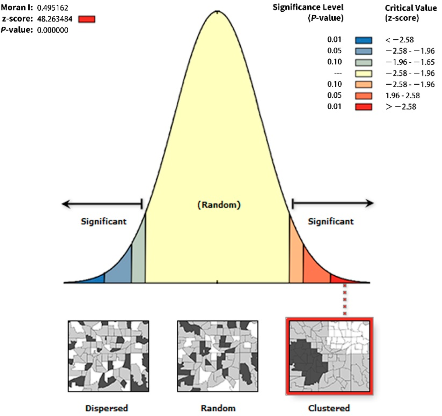
This article first calculates the global Moran’s I index to measure the degree of spatial autocorrelation of the benchmark rent of the sample rental housing community. Using Matlab software, the Moran’s I coefficient of $\ln P$ is calculated to be 0.4952, and the p value is 0.0000, which has passed the significant value at the 1% level. The test, and the Z score, is 48.26, which is significantly positive, indicating that the benchmark rent has spatial effects and positive spatial autocorrelation (Figure 3).

There are spatial effects caused by heterogeneity and dependence between spatial data, but the relationship between them is ignored in the classic regression analysis model (OLS). After Moran’s I index has verified that there is a certain degree of spatial correlation between the benchmark rent of rental housing and its influencing factors, it is necessary to determine the most appropriate spatial measurement model for analysis. This paper selects the appropriate model through LaGrange test. As Moran’s I test is significant when the maximum likelihood LMLAG test is more significant than the LMERR test, this article chooses the spatial lag model; otherwise, the spatial error model is chosen.

It can be seen from

Table 4. LM statistics test results of the housing rent space weight model.

Testing Method	LMERR	LMLAG	R-LMERR	R-LMLAG
Statistics	2989.4869	2617.5919	920.6184	548.8234
p value	0.0000	0.0000	0.0000	0.0000

that LMERR > LMLAG, R-LMERR > R-LMLAG for the economic distance spatial weight model, and the test values all pass the significance test at the 1% level, whether it is a LaGrange test or a robustness test. The spatial error model based on the weight of the rental housing price feature is statistically more significant than the spatial lag model, so this article chooses the spatial error model as a method for further research.

At the same time, we compared the estimation results of the spatial lag model (SLM) and the spatial error model (SEM) (Lin Guangping, 2014), as shown in

Table 5. Spatial lag model (SLM) and spatial error model (SEM) of benchmark rent.

Benchmark Rent (Ln-Rent)		SLM		SEM
		Coefficient	t	Coefficient	t
Community attributes	Age	−0.034	−0.806	−0.006	−0.146
	FAR	−0.181	−0.332	0.066	0.343
	Greening	−0.161	−0.019	2.948	0.343
Employment accessibility	D-job	−3.232 ***	−5.285	−10.847 ***	−8.145
	C-job	1.805 ***	5.226	4.292 ***	14.897
Location traffic	Bus	−2.443 ***	−2.915	−1.288 ***	−0.98
	Subway	−1.159 **	−2.133	−0.758 **	−1.059
Public Service	Park	−0.466	−0.997	−0.373	−0.654
	Hospital	−1.204 **	−2.512	−2.021 **	−2.628
	service	1.000 *	1.452	0.118 *	0.119
	Pschool	−1.951 **	−4.256	−4.134 **	−5.186
Constant		69.005 ***	5.496	174.284 ***	13.628
ρ/λ		0.676		0.689
R2		0.4176		0.5375
LogL		−25,763.867		−25,827.597
LM		2617.5919		5172.9086
Sample size		5980		5980

Note: *, **, and *** are significant at 10%, 5%, and 1% level, respectively.

. In the process of setting the spatial weight matrix, since the sample studied in this paper is a point element, it has the characteristics of wide spatial distribution and local aggregation. The k-order neighbor weight matrix is defined, and the k = 1:20 neighbor matrix result is calculated by the robustness test of the maximum likelihood value sets of the optimal number of neighbors. We uses the maximum likelihood method to estimate the regression model and took k = 13.

Comparing the Log likelihood (LogL) and Lagrange multiplier (LM) values of the spatial lag model (SLM) and the spatial error model (SEM), we can see that the values of the spatial error model (the results of SEM) are better than those of the spatial lag model (SLM), indicating that the factors that affect the benchmark rent of rental housing communities are also potential factors. Compared with the OLS regression model, the spatial error model (SEM) model, after introducing spatial effects, did not impact the significance level of the variables, parks, and district key points, and public school district housing had no significant impact on the benchmark rent.

The regression results show that the community attributes (construction year, plot ratio, and greening rate) have no significant impact on the benchmark rent, indicating that tenants consider community attributes to be critical when choosing a house to rent. The degree of employment accessibility greatly influences the benchmark rent, indicating that tenants should first consider commuting time with their employer when choosing a house. The degree of influence of employment opportunities is greater than the degree of distance to the employment center. Among the location characteristics, the benchmark rent is highly dependent on the bus station, showing that the farther the distance to the nearest bus station, the lower the benchmark rent price, and the influence of the subway station is relatively less obvious. Regarding public service facilities, whether it is the least square method (OLS) model, the spatial lag model (SLM), or the spatial error model (SEM), parks and supermarkets have no significant impact on the benchmark rent, so we will not elaborate on the park variables here. The regression coefficient of the third-class hospitals is negative, indicating that third-class hospitals have a specific role in increasing the benchmark rent, especially due to the fact that society is aging, the elderly are more willing to live nearby to third-class hospitals to facilitate medical treatment, and that the migrant population comes to Beijing for medical treatment, these groups also have a great demand for leasing; therefore, without considering other variables, the benchmark rents of communities near third-class hospitals are often higher. Moreover, in order to facilitate school-age children going to school, many parents tend to rent houses near key primary schools, which has increased the benchmark rent of communities near key primary schools to a certain extent.

3.3. Market Benchmark Rent Measurement Method

The benchmark rent measurement method can be summarized in the following four points:

• The construction year, floor area ratio, and greening ratio have no significant impact on rental housing’s benchmark rent.
• The employment center has a relatively large impact on the benchmark rent. The closer to the job center, the lower the commuting cost could be, and the higher the benchmark housing rent.
• The park has no significant impact on the benchmark rent. For renters, most of them are unable to buy with such high housing prices in first-tier cities, and they are struggling to survive. In addition to renting in high-priced housing communities, they should consider the residential function of the house when renting, whereas parks that mainly have leisure functions are not important factors to consider. The impact of living facilities (supermarkets, shopping malls) and other facilities are also not significant, indicating that e-commerce has changed people’s lifestyles.
• The housing in key school districts of Beijing can be said to make it easy for children to go to school. Key school districts have a clear positive impact on the benchmark rent. It further confirms that the housing rental market is dominated by residential employment.

Based on the comparative study of several models, the most suitable market benchmark rent measurement method is determined as the spatial error model (SEM):

$$\mathrm{y}={{\displaystyle \sum }}_{q=1}^Q{X}_{iq}{\beta }_q+\mathsf{\lambda }{{\displaystyle \sum }}_{j=1}^n{\mathrm{W}}_{ij}{\mathsf{\epsilon }}_j+{\mu }_i,$$

(4)

where ${\mathsf{\lambda }\mathrm{W}}_{ij}+\mathsf{\epsilon }$ is the disturbance term, which expresses those not included in X (the index system that affects the benchmark rent).

For the missing variable that has an impact on the dependent variable y (benchmark rent), the regression coefficients must be substituted:

$$\ln {\mathrm{rent}}_i=174.284-0.006{\mathrm{Age}}_i+0.066{\mathrm{FAR}}_i+2.948{\mathrm{Greening}}_i-10.847{\mathrm{Djob}}_i+4.292{\mathrm{Cjob}}_i-1.288{\mathrm{Bus}}_i-0.758{\mathrm{Subway}}_i-0.373{\mathrm{Park}}_i-2.021{\mathrm{Hospital}}_i+0.118{\mathrm{Service}}_i-4.134{\mathrm{Pschool}}_i+0.689{\mathrm{W}}_{ij}+{\mu }_i$$

(5)

4. Conclusions

The factors affecting the benchmark rent of market-based rental housing have spatial differentiation. In other words, the OLS price feature model ignores the spatial impact, but the benchmark housing rent and its influencing factors are data with spatial mutual influence relationships, which will be affected by spatial relationships caused by spatial heterogeneity and dependence. After LaGrange and robustness tests, it is found that the spatial error model (SEM) is better than traditional models, which finally allows the benchmark rent measurement method for market rental housing to be obtained.

The dominant players in the housing rental market are mainly low- and middle-income groups and a small number of high-income groups. There are a different investment and speculative needs in the housing market [11,17,36]. The rental housing market meets the rigid housing needs of various groups of people, which reflects the crowd’s real living demand. Moreover, the benchmark rent can be attributed to four major factors: community attributes, employment attributes, location attributes, and public services. The characteristic price model is based on OLS regression which explains the average sense of influencing factors. The spatial measurement model that introduces spatial effects has a significantly higher interpretation strength than the characteristic price model, indicating that the benchmark housing rent has spatial spillover effects. Community attributes (construction year, plot ratio, greening rate) have no significant impact on the benchmark rent, indicating that most of the tenants are low- and middle-income households and are not sensitive to the community’s quality. The benchmark housing rent is very sensitive to commuting costs. The more bus stations and subway stations nearby, the closer the distance to the job center, the more job opportunities there are, the lower the commuting cost, and the higher the benchmark housing rent. Parks have no significant impact on the benchmark housing rent because most renters cannot afford such high housing prices in first-tier cities and are struggling to survive. When renting a house, more consideration should be given to the residential function of the house, whereas parks, which mainly have leisure functions, are not important factors to consider. The impact of key elementary schools on the benchmark rent is relatively obvious, indicating that Beijing’s high transportation cost is due to nearby schools’ rental demand.

The main groups involved in the rental housing market are mainly low- and middle-income groups and a small number of high-income groups. Unlike the investment and speculative demand that exists in the housing sale and purchase market, the rental housing market caters to the rigid housing needs of various groups of people. The benchmark rent measurement method helps real estate developers to scientifically and reasonably measure the cost-benefit and cost-recovery period of investing in rental housing to a greater extent, and to scientifically and reasonably build and supply rental housing to a greater extent. It also helps residents in the rental housing market to make the most scientific decisions based on their ability to pay, the work–life balance, and amenities. Furthermore, it will help them realize a reasonable and effective screening of rental housing when their income changes. For policy makers, benchmark rents can provide a scientific guideline for the rental housing market, establishing clear standards for rent setting and regulatory controls. We use the Beijing rental housing market as the pilot city for the study, and its benchmark rent determination method for market-based rental housing can be extended further to other cities.

References

- Shi, W.; Chen, J.; Wang, H. Affordable Housing Policy in China: New Developments and New Challenges. Habitat Int. 2016, 54, 224–233. [Google Scholar] [CrossRef] [Green Version]
- Kemeny, J.; Kersloot, J.; Thalmann, P. Non-Profit Housing Influencing, Leading and Dominating the Unitary Rental Market: Three Case Studies. Hous. Stud. 2005, 20, 855–872. [Google Scholar] [CrossRef]
- Gu, S.; Li, H. Improve the Rental Market and Construct a Multi-level Housing System. Theory J. 2013, 1, 59–63. [Google Scholar] [CrossRef]
- Zhang, C.; Jia, S.; Yang, R. Housing Affordability and Housing Vacancy in China: The Role of Income Inequality. J. Hous. Econ. 2016, 33, 4–14. [Google Scholar] [CrossRef]
- Li, D.; Chen, H.; Hui, E.C.; Xiao, C.; Cui, Q.; Li, Q. A Real Option-Based Valuation Model for Privately-Owned Public Rental Housing Projects in China. Habitat Int. 2014, 43, 125–132. [Google Scholar] [CrossRef]
- Huang, Y. Housing Markets, Government Behaviors, and Housing Choice: A Case Study of Three Cities in China. Environ. Plan. A 2004, 36, 45–68. [Google Scholar] [CrossRef]
- Wu, W. Sources of Migrant Housing Disadvantage in Urban China. Environ. Plan. A 2004, 36, 1285–1304. [Google Scholar] [CrossRef] [Green Version]
- Yuan, J.; Li, W.; Zheng, X.; Skibniewski, M.J. Improving Operation Performance of Public Rental Housing Delivery by PPPs in China. J. Manag. Eng. 2018, 34, 04018015. [Google Scholar] [CrossRef]
- Li, J.; Li, D.; Ning, X.; Sun, J.; Du, H. Residential Satisfaction among Resettled Tenants in Public Rental Housing in Wuhan, China. J. Hous. Built Environ. 2019, 34, 1125–1148. [Google Scholar] [CrossRef]
- Li, J.; Stehlik, M.; Wang, Y. Assessment of Barriers to Public Rental Housing Exits: Evidence from Tenants in Beijing, China. Cities 2019, 87, 153–165. [Google Scholar] [CrossRef]
- Luo, D.; van der Heijden, H.; Boelhouwer, P.J. Policy Design and Implementation of a New Public Rental Housing Management Scheme in China: A Step Forward or an Uncertain Fate? Sustainability 2020, 12, 6090. [Google Scholar] [CrossRef]
- Hosios, A.J.; Pesando, J.E. Measuring Prices in Resale Housing Markets in Canada: Evidence and Implications. J. Hous. Econ. 1991, 1, 303–317. [Google Scholar] [CrossRef]
- Xie, S.; Chen, J. Beyond Homeownership: Housing Conditions, Housing Support and Rural Migrant Urban Settlement Intentions in China. Cities 2018, 78, 76–86. [Google Scholar] [CrossRef]
- Sun, T. Spatial Mismatch between Residences and Jobs by Sectors in Beijing and Its Explanations. Geogr. Res. 2015, 34, 351–363. [Google Scholar] [CrossRef]
- Morano, P.; Guarini, M.R.; Sica, F.; Anelli, D. Ecosystem Services and Land Take. A Composite Indicator for the Assessment of Sustainable Urban Projects. In Proceedings of the International Conference on Computational Science and Its Applications, Cagliari, Italy, 13–16 September 2021; Springer: Berlin/Heidelberg, Germany, 2021; pp. 210–225.
- Garang, Z.; Wu, C.; Li, G.; Zhuo, Y.; Xu, Z. Spatio-Temporal Non-Stationarity and Its Influencing Factors of Commercial Land Price: A Case Study of Hangzhou, China. Land 2021, 10, 317. [Google Scholar] [CrossRef]
- Cui, N.; Gu, H.; Shen, T.; Feng, C. The Impact of Micro-Level Influencing Factors on Home Value: A Housing Price-Rent Comparison. Sustainability 2018, 10, 4343. [Google Scholar] [CrossRef] [Green Version]
- Kim, A.M. The Extreme Primacy of Location: Beijing’s Underground Rental Housing Market. Cities 2016, 52, 148–158. [Google Scholar] [CrossRef] [Green Version]
- Guntermann, K.L.; Norrbin, S. Explaining the Variability of Apartment Rents. Real Estate Econ. 1987, 15, 321–340. [Google Scholar] [CrossRef]
- Björklund, K.; Klingborg, K. Correlation between Negotiated Rents and Neighbourhood Quality: A Case Study of Two Cities in Sweden. Hous. Stud. 2005, 20, 627–647. [Google Scholar] [CrossRef]
- Yusuf, A.A.; Resosudarmo, B.P. Does Clean Air Matter in Developing Countries’ Megacities? A Hedonic Price Analysis of the Jakarta Housing Market, Indonesia. Ecol. Econ. 2009, 68, 1398–1407. [Google Scholar] [CrossRef]
- Wang, S. The Supply Side of First-Tier Cities Rentals is the Core Conflict, and Which Cities Are Likely to Pass on the Property Tax Pressure? SWS Research: Shanghai, China, 2018. [Google Scholar]
- Wu, W. Migrant Housing in Urban China: Choices and Constraints. Urban Aff. Rev. 2002, 38, 90–119. [Google Scholar] [CrossRef]
- John, B. Mass Transportation, Apartment Rent and Property Values. J. Real Estate Res. 1996, 12, 1–8. [Google Scholar] [CrossRef]
- Frew, J.; Wilson, B. Estimating the Connection between Location and Property Value. J. Real Estate Pract. Educ. 2002, 5, 17–25. [Google Scholar] [CrossRef]
- Chau, K.W.; Chin, T.L. A Critical Review of Literature on the Hedonic Price Model; International Journal for Housing Science and Its Applications. Int. J. Hous. Sci. Its Appl. 2003, 27, 145–165. Available online: https://ssrn.com/abstract=2073594 (accessed on 29 April 2022).
- Ding, C. The Benchmark Land Price System and Urban Land Use Efficiency in China. Chin. Geogr. Sci. 2001, 11, 306–314. [Google Scholar] [CrossRef]
- Hu, R.; Wang, Z.; Qiu, F. Identification and Function Orientation of Employment Centers in Beijing Based on the Census Unit Analyzing. Hum. Geogr. 2016, 31, 58–65. [Google Scholar] [CrossRef]
- He, C.; Wang, Z.; Guo, H.; Sheng, H.; Zhou, R.; Yang, Y. Driving Forces Analysis for Residential Housing Price in Beijing. Procedia Environ. Sci. 2010, 2, 925–936. [Google Scholar] [CrossRef] [Green Version]
- Davidoff, T. Labor Income, Housing Prices, and Homeownership. J. Urban Econ. 2006, 59, 209–235. [Google Scholar] [CrossRef] [Green Version]
- Gabriel, S.A.; Mattey, J.P.; Wascher, W.L. Compensating Differentials and Evolution in the Quality-of-Life among U.S. States. Reg. Sci. Urban Econ. 2003, 33, 619–649. [Google Scholar] [CrossRef]
- Roback, J. Wages, Rents, and the Quality of Life. J. Political Econ. 1982, 90, 1257–1278. [Google Scholar] [CrossRef]
- Balta, M.O.; Eke, F. Spatial Reflection of Urban Planning in Metropolitan Areas and Urban Rent; a Case Study of Cayyolu, Ankara. Eur. Plan. Stud. 2011, 19, 1817–1838. [Google Scholar] [CrossRef]
- Sun, T.; Fan, Y.; Qi, Y. Beijing Job Accessibility Map—Transit: A Joint Initiative Between the Global Transit Innovations at the University of Minnesota and the School of Government at the Peking University; University of Minnesota: Minneapolis, MN, USA, 2015. [Google Scholar]
- Wu, J.; Adams, R.M.; Plantinga, A.J. Amenities in an Urban Equilibrium Model: Residential Development in Portland, Oregon. Land Econ. 2004, 80, 19–32. [Google Scholar] [CrossRef]
- Zhou, J.; Musterd, S. Housing Preferences and Access to Public Rental Housing among Migrants in Chongqing, China. Habitat Int. 2018, 79, 42–50. [Google Scholar] [CrossRef]
Figure 1.
Distribution of market-leased communities in Beijing.
Figure 2.
Employment opportunities within 60 min in Beijing.
Figure 3.
Space autocorrelation report of benchmark rent.