Evaluation of the Effect of Average Annual Temperatures in Slovakia between 1971 and 2020 on Stresses in Rigid Pavements

Abstract

The scientific community in Central Europe often discusses the extent to which temperature changes over the last two decades have contributed to changing the stresses induced in structures. In the field of road and environmental engineering, this question is especially pertinent for pavements. The pavement structure must first be defined methodologically by identifying and defining the types of parameters that change with time. Additionally, it is important to identify the areas of Central Europe that are most affected by climate change. The most important parameters must be described statistically for these areas. Slovakia is one of the countries that may be able to contribute to the solution of this issue due to its location in the middle of Europe. This paper provides a statistical analysis for the period from 1971 to 2020 in Slovakia. A concrete pavement, which is the most commonly used type of pavement, must be used as an example to numerical assess the situation. The conclusions and discussion in this scientific field are directed towards the evaluation of the measurement results in the context of the designed pavement composition and the calculations using the different methods specified in the standards.

1. Introduction

Increased average annual temperatures are linked to global warming, a worldwide problem. Central Europe (CE) is a very specific area. It is characterized throughout by a wide range of temperature zones, as well as different traffic loads and infrastructure. There has been a significant urbanization process in these countries that influences temperature changes. This process involves covering the Earth’s surface with different types of roads. As a result, grassland areas are being reduced. This effect is called the urban heat island effect (UHI) [1,2]. It is related to the increasing surface temperature of concrete pavements and their accumulation capacity. A rigid pavement and its surroundings form a single, interdependent system. Climate change (temperature, precipitation, groundwater level, freezing and thawing cycles) influences the structural properties and interactions of this system [3,4,5,6].

The most significant factor is temperature change, which can be observed in the evolution of the annual mean temperature in Slovakia between 1971 and 2020. Temperature trends in these years are comparable to those of the Visegrad Four. Currently, this development can hardly be slowed [7,8]; therefore, it is necessary to analyze the phenomena that arise as a result of these changes. Rigid pavements are increasingly loaded with different types of traffic. Vehicle loads induce stresses and deformations in the cement-concrete slab (CCS). The CCS is influenced by both the traffic load and the temperatures of the individual pavement layers at the same time. The influence of these factors on the properties of the pavement materials used is important. It is also important to determine how the whole structure will respond to these stresses. To study this, numerical modelling is considered the most appropriate method in many developed countries around the world. It is applied in the design of CCS in pavement construction, as well as in the assessment of its structural response [9].

2. The Average Annual Temperature in Slovakia, Located in CE

Past studies have presented results on the impacts of temperature changes on pavement response [10,11]. Particular attention has been paid to the assessment of cement concrete pavements in Central Europe (CE). To begin with, we would like to define the term CE, which may seem straightforward at first sight but in reality is not. The authors therefore present, in a separate section, the development, the currently established perception, and their definition of CE [12,13,14,15,16]. The authors of [17] show that the 20 years between 1988 and 2008 were very likely the warmest 20-year period in CE (Czech Republic, Germany, Switzerland, Poland, Slovakia, Austria, Hungary, and the part of Ukraine) since 1500.

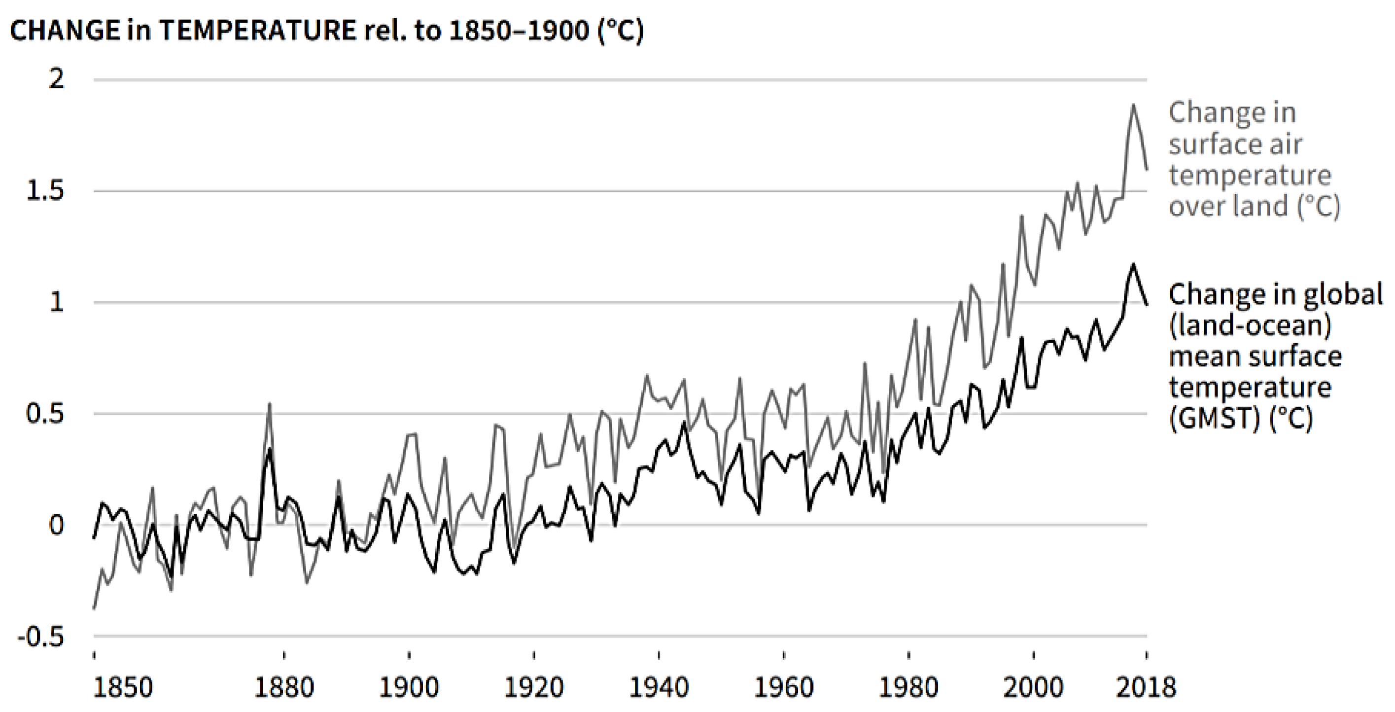
According to [18], the Earth’s temperature rose by 0.08 °C per decade after 1880, and the rate of warming over the past 40 years is more than twice that: 0.18 °C per decade since 1981. The year 2020 was the second-warmest year on record based on NOAA’s temperature data, and for land areas it was the warmest on record. Averaged across land and ocean, the 2020 surface temperature was 0.98 °C warmer than the twentieth-century average of 13.9 °C, and 1.19 °C warmer than the pre-industrial period (1880–1900). The authors of [19] revealed surface warming and its elevation dependency using daily temperature data from 745 meteorological stations in China during 1963–2012. We calculated the temperature trends for individual stations and then summarized trends for three elevation zones at different latitudes. It was found that there was a general warming trend in agreement with global warming, with a warming rate of 0.26 °C/decade. In [20], warming from pre-industrial levels to the decade of 2006–2015 was assessed to be 0.87 °C (likely between 0.75 °C and 0.99 °C). The surface temperature (ST) over India increased by ~0.055 K/decade during 1860–2005 and this follows the global warming trend [21]. The transition pathways in the 2015 Paris Agreement calls for countries to pursue efforts to limit the global mean temperature rise to 1.5 °C [22]. The transition pathways that can meet such a target have not, however, been extensively explored [23]. Temperatures also, together with the dominant influence of traffic, have an effect on the propagation of road traffic noise and redistribution and the seasonal variations in particular matter induced by traffic [24,25].

In many developed countries around the world, numerical modelling is the most commonly used method. This method is used in the design of the CCS in the pavement structure, as well as in the assessment of the response of the structure and the analysis of the resulting stresses. The response can be divided into stresses and strains. For this reason, this article is supplemented with an example of a real pavement numerical analysis using the finite element method (FEM) [26].

2.1. Impact of High Temperatures of Cement Concrete on Its Properties

According to the Intergovernmental Panel on Climate Change (IPCC), the United Nations body for assessing the science related to climate change, climate change without any additional efforts to mitigate it will lead to a global mean temperature rise of anywhere from 2 °C to 7.8 °C by 2100 relative to the 1850–1900 reference period (Figure 1) [3,4,5].

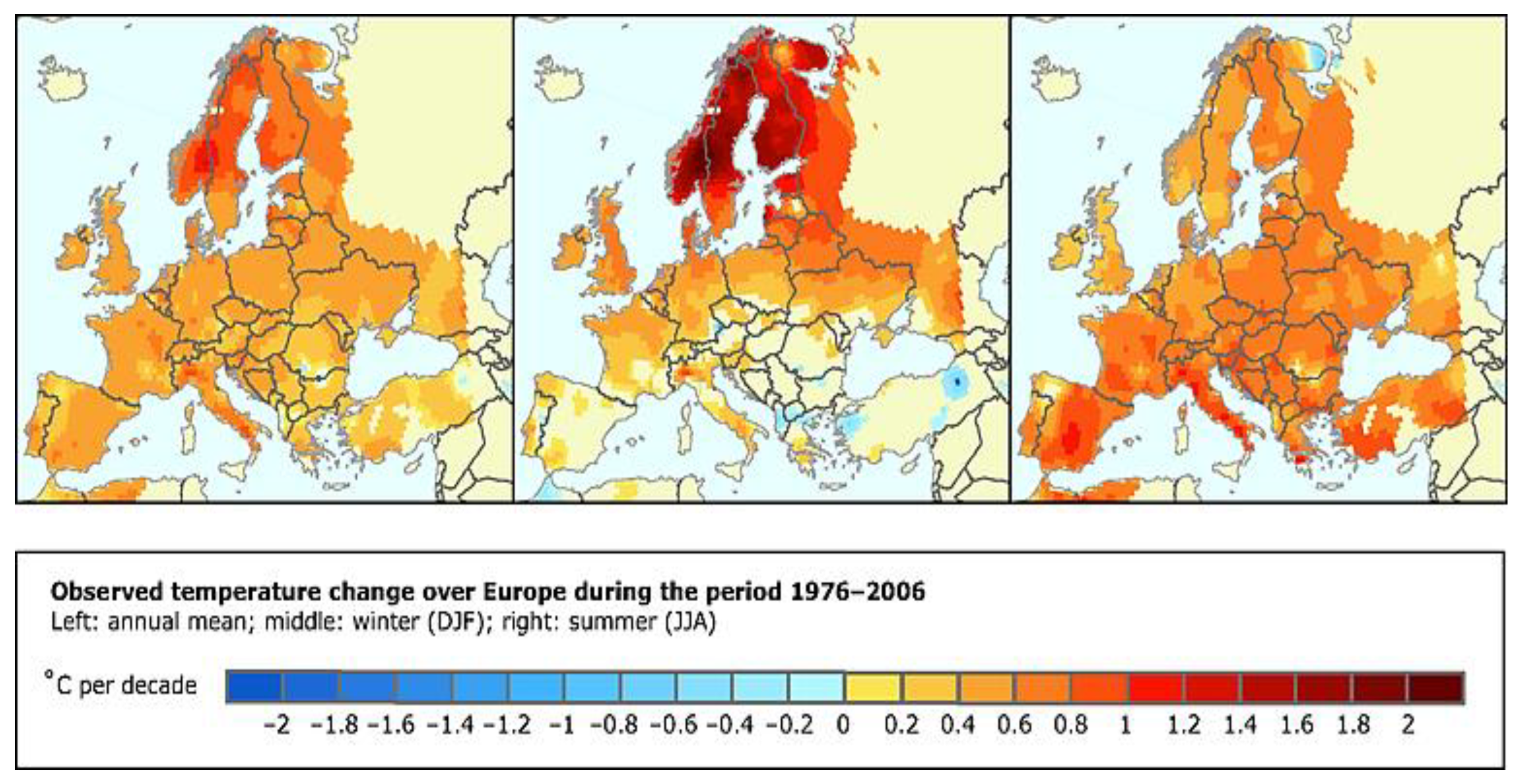
According to European Environment Agency (EEA), an agency of the EU, data from 1976 to 2006 [6], the following average warming values occurred in CE: annual mean 0.4 to 0.6 °C, summer 0.2 to 0.4 °C, winter 0.6 to 0.8 °C (Figure 2). The EEA provides sound, independent information on Europe’s environment through the provision of timely, targeted, relevant, and reliable information to policymaking agents [17].

We note with grave concern the significant gap between the aggregate effect of parties’ mitigation pledges in terms of global annual emissions of greenhouse gases by 2020 and aggregate emission pathways consistent with having a likely chance of holding the increase in global average temperature below 2 degrees Celsius or 1.5 degrees Celsius above pre-industrial levels [27]. High concrete temperatures increase the rate of hydration, thermal stresses, permeability, and the tendency towards dry shrinkage cracking and decrease long-term concrete strength and durability as a result of said cracking. Data analysis from the Texas Rigid Pavement database showed that these disorders occur especially in the case of using aggregates: limestone and siliceous river gravel [28].

The results of the analysis emphasize the importance of concrete temperature control during concrete pavement construction in hot weather conditions. Most states specify a maximum concrete temperature at placement to mitigate the detrimental effects of placement during hot weather. Changes in ambient air temperature during concrete placement are associated with the risk of early cracking. This risk is much greater when temperatures drop from 21 °C to 7 °C than when temperatures drop from 38 °C to 24 °C. Further information can be found in [29]. Concern has been expressed in Florida that, because of a nonlinear temperature gradient in a Portland cement concrete (PCC) pavement, internal stresses could be developed such that the life of the pavement would be seriously reduced. These results were compared with those obtained from the AASHO Test Road and with Bergstrom’s prediction method. The results indicated that the nonlinearity of the temperature gradient in a PCC pavement did not have a significant impact on its performance [30]. The territory of Slovakia is in CE at the interface of the parts of the continent that are influenced by continental and oceanic climates. Apart from traffic load, a change in climatic conditions is one of the constant external factors with adverse effects on the physical and mechanical properties of different structural multi-layers in pavements. The 20th century CE temperature increase (+1.2 °C) evolved stepwise with the first peak near 1950 and the second increase (1.3) starting in the 1970s [31].

Since the 19th century, Slovakia has experienced a growth in its annual average temperature of about 1.5 °C, precipitation changes, decreased relative humidity, and changes in solar radiation [7].

2.2. Delimitation of the Territory of Central Europe

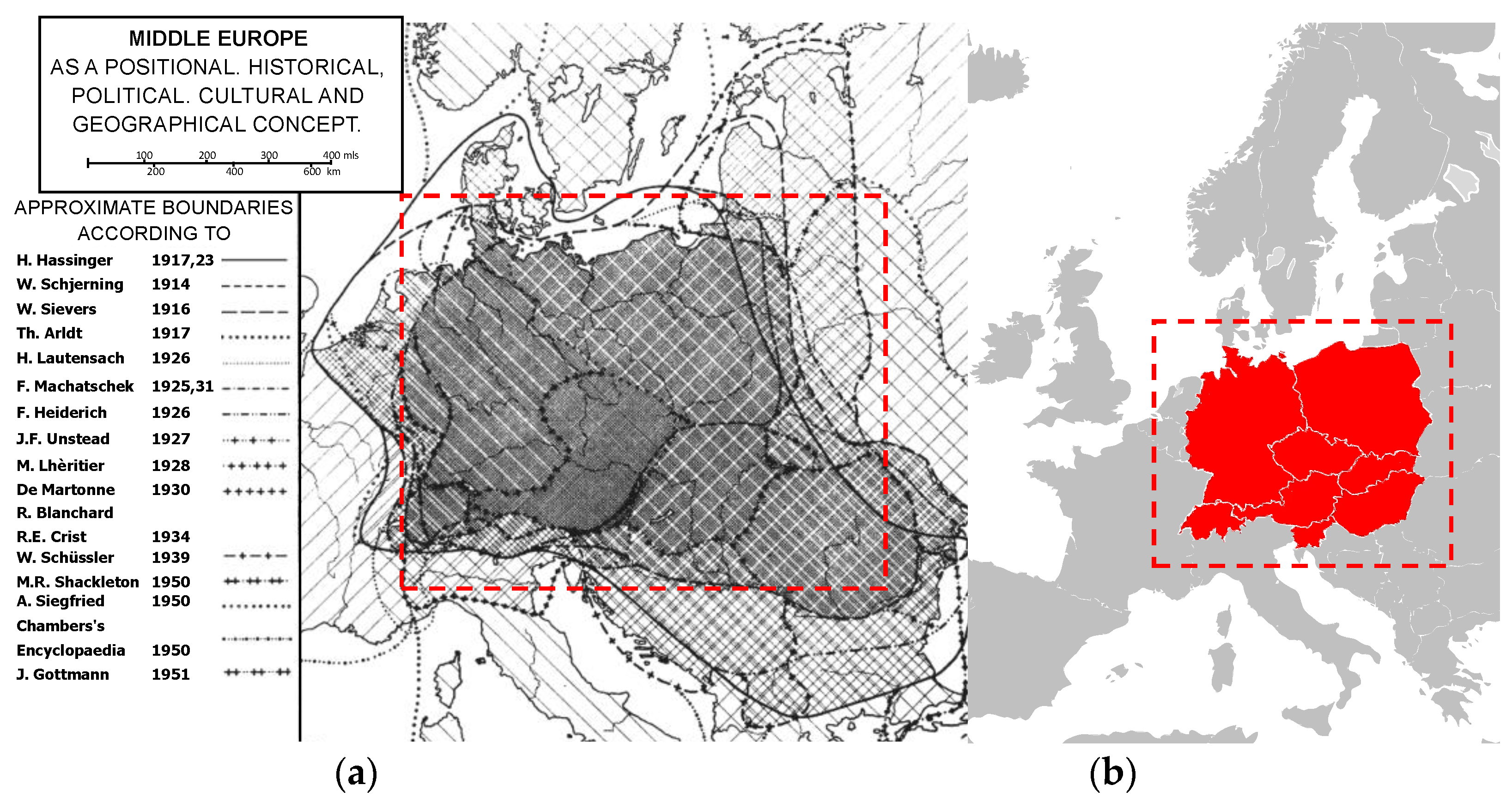
Figure 3 [12,15] presents the development and the present understanding of the territory of Central Europe (for clarity, this part is highlighted in Figure 3) for which the authors apply objective research results. Many geographical terms either lack or come to lack a precise meaning and the term Central Europe is a typical example. The development of the perception of Central Europe (Middle Europe, Mitteleuropa, Europe Centrale, Central Europe, etc.) according to various authors is shown in Figure 3a.

The graphic borders of Central Europe, shown in Figure 3a, were available only in some cases. In other cases, they are drawn based on written descriptions in relevant texts. The location of the geographical center of Europe depends on the definition of the borders of Europe, mainly whether remote islands are included to define the extreme points of Europe, and on the method of calculating the final result. Thus, several places claim to house this hypothetical center: the town of Kremnické Bane or the neighboring town Krahule, near Kremnica, in Central Slovakia; the small town of Rakhiv or the town of Dilove, near Rakhiv, in Western Ukraine; the town of Girija, near Vilnius, in Lithuania; a point on the island of Saaremaa in Estonia; a point near Polotsk, or in Vitebsk, or near Babruysk, or the nearby lake Sho in Belarus; and a point near the town of Tallya, in Northeastern Hungary (Figure 4). The towns of Krahule and Kremnicke Bane are generally understood by the Slovak authors as the geometric center of Continental Europe, as well as by foreign authors [13,14].

In the following sections, the development of the average annual air temperature at 10 climatological stations in Slovakia as a Central European country is presented for this reason.

3. Development of the Average Annual Air Temperature of 10 Climatological Stations in Slovakia with an Altitude of 115 to 858 above Sea Level for the Period 1971 to 2020

Regarding research on correlation dependencies, we briefly describe the basic statistics—correlation coefficient and coefficient of determination. In mathematics, the Spearman correlation coefficient is usually used to quantify how much two columns of data linearly depend on each other. Charles Edward Spearman (1863–1945) was an English psychologist known for his work on statistics as a pioneer of factor analysis and Spearman’s rank correlation coefficient. The values of Spearman’s rank correlation coefficient according to

Table 1. Spearman and Pearson’s correlation coefficients and their degrees and interpretation. The table uses data from [38,39].

Spearman Correlation Coefficient ρ		Pearson’s Correlation Coefficient
Grading Standards	Correlation Degree	Size of Correlation	Interpretation
ρ = 0	No correlation	0.9 to 1.0 (−0.9 to −1.0)	Very high positive (negative) correlation
00 < |ρ| ≤ 0.19	Very week	0.7 to 0.9 (−0.7 to −0.9)	High positive (negative) correlation
0.20 < |ρ| ≤ 0.39	Weak	0.5 to 0.7 (−0.5 to −0.7)	Moderate positive (negative) correlation
0.40 < |ρ| ≤ 0.59	Moderate	0.3 to 0.5 (−0.3 to −0.5)	Low positive (negative) correlation
0.60 < |ρ| ≤ 0.79	Strong	0.0 to 0.3 (−0.0 to −0.3)	Negligible correlation
0.80 < |ρ| ≤ 0.99	Very strong
1.00	Monotonic

are most often mentioned in the technical, as well as behavioral, literature [32,33,34]. Karl Pearson built on Francis Galton’s research, and Auguste Bravais developed and published the mathematical formula in 1844 [35,36,37].

Given a pair of random variables (X,Y), the equation for Pearson’s correlation coefficient R(X,Y) is:

$$R\left(X,Y\right)=\frac{{{\displaystyle \sum }}_{i=1}^n{X}_i{Y}_i-n\overline{X}\overline{Y}}{\sqrt{\left({{\displaystyle \sum }}_{i=1}^n{X}_i^2-n{\overline{X}}^2\right)\left({{\displaystyle \sum }}_{i=1}^n{Y}_i^2-n{\overline{Y}}^2\right)}}$$

(1)

where $cov\left(X,Y\right)$ is the covariance; ${\sigma }_X$ and ${\sigma }_Y$are the standard deviations of $X$ and $Y,$ respectively; $n$ is the sample size; $X_i,Y_i$ are the individual sample points; and $\overline{X}, \overline{Y}$are the sample means. The correlation coefficient ranges from −1 to 1. The value $R\left(X,Y\right)=0$implies that there is no linear dependency between variables$\left(X,Y\right)$. A relatively high correlation coefficient means that there is a high linear dependency between the variables. This does not necessarily mean that there is also a high causal dependency. The degree of causal dependence is expressed by the coefficient of determination $R^2,$a key output in regression analysis. It is the square of the correlation coefficient between variables based on the sample values. It gives valid results when the observations are evaluated correctly without measurement errors. Based on the coefficient of determination, we can assess to what extent the regression model fits the observed data.

3.1. Correlation Dependencies of Average Annual Temperatures T_a for the Period 1971–2020

In this section, the authors present the latest research results in the field of the objective correlation dependences of the average annual temperature from the altitude of the assessed pavement. For practical purposes, the flow of daily temperature is expressed by the average daily temperature, calculated as shown in Equation (2):

$$T_d=\frac{\left(T_7+T_{14}+2\cdot T_{21}\right)}{4}$$

(2)

where indexes 7, 14, and 21 are the times at which air temperature T is measured. Considering the standard in Equation (2), the average daily air temperature is calculated as the average of the four measured values T₇, T₁₄, and twice the value of T₂₁. Twice the value of T₂₁ is included because there are no night measurements available [40]. The temperature of earth structures changes along with the change in air temperature. Average annual air temperature T_a is expressed by the formula:

$$T_a={\displaystyle \sum }_{i=1}^{365}{T}_{d,i}/365$$

(3)

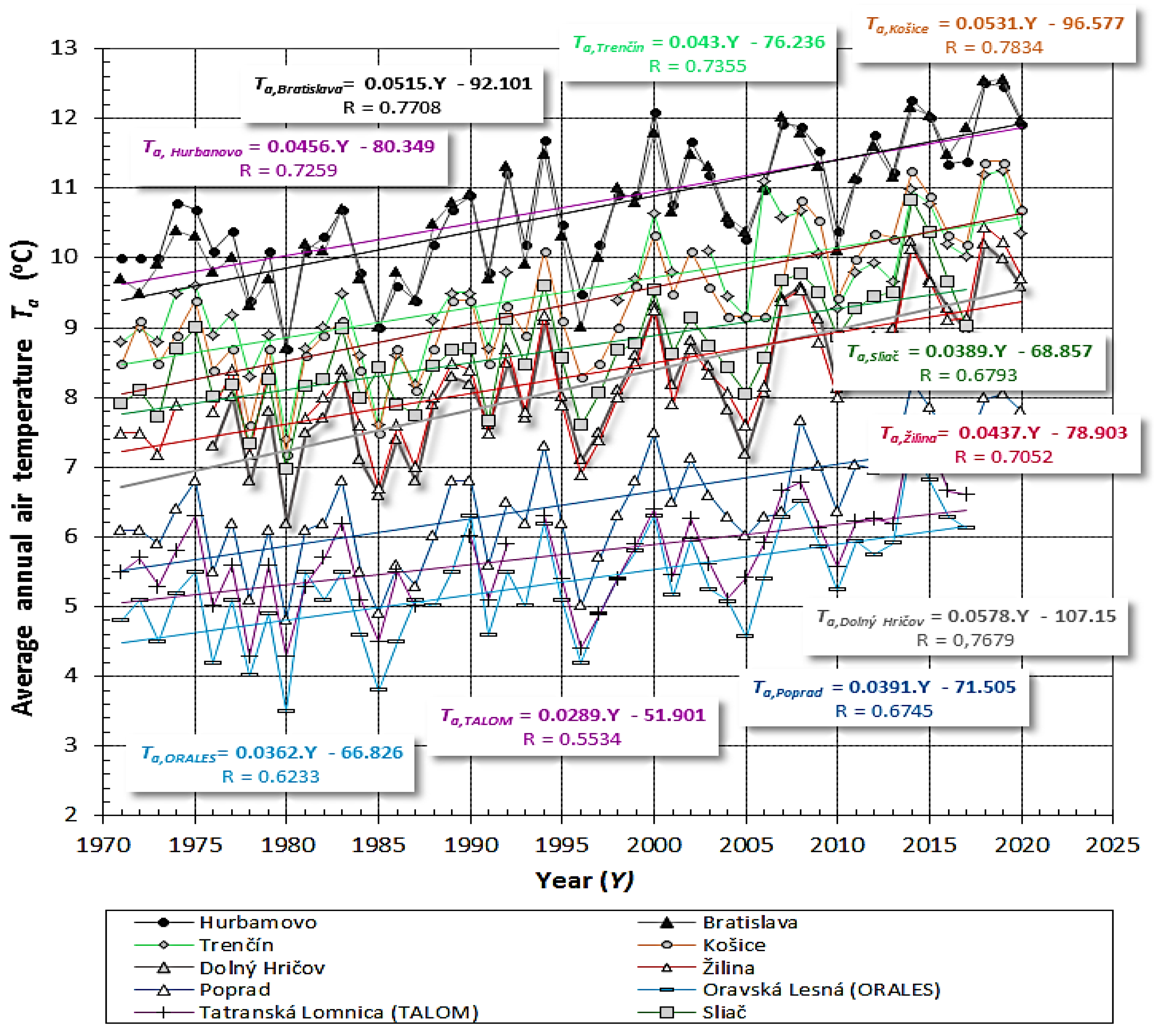
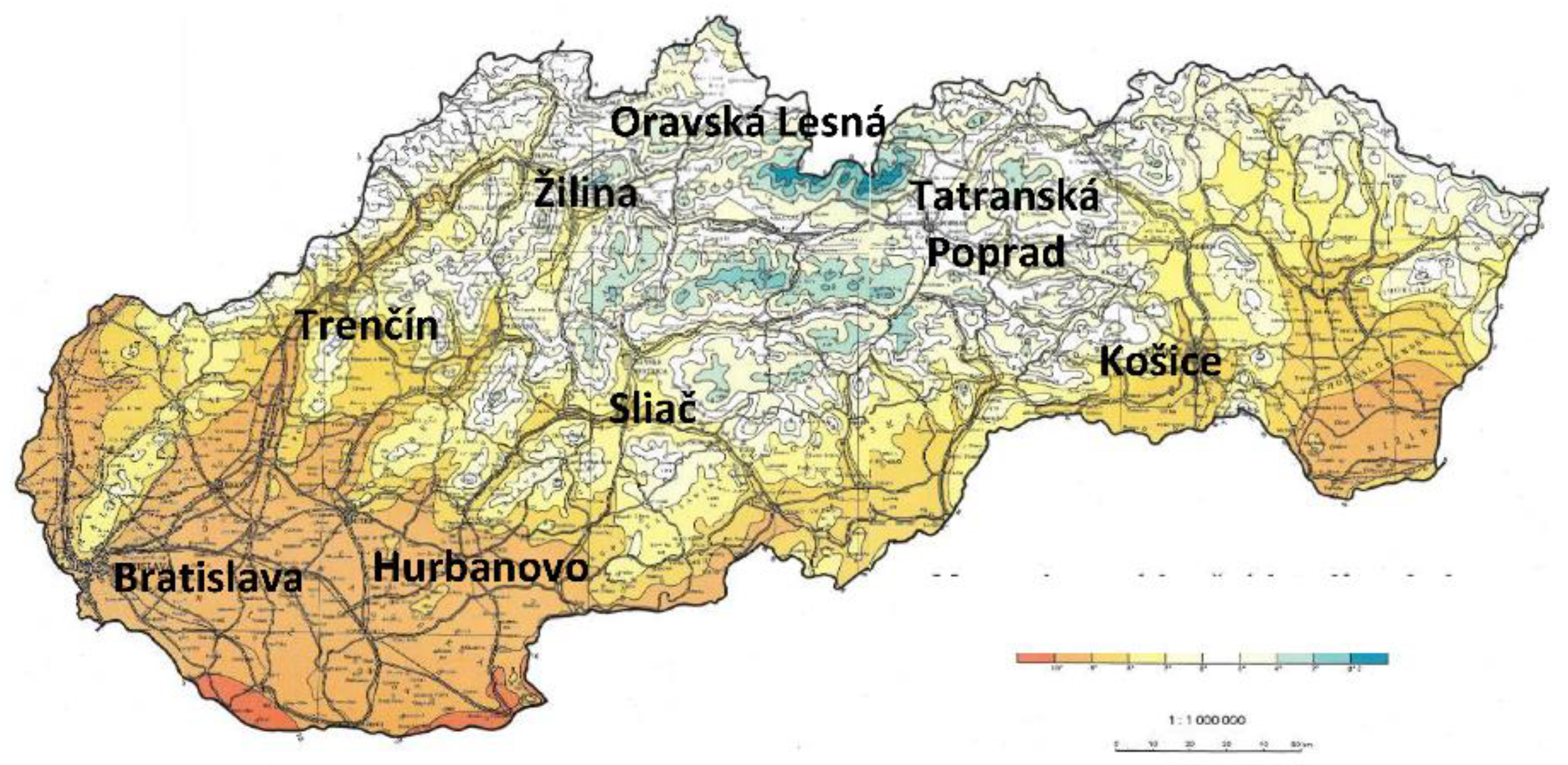
Air temperature has a cyclical character repeated in daily and annual cycles with an approximately sinusoidal shape. Figure 4 presents the mean annual temperatures T_a of 11 climatological stations with significantly different altitudes; from Hurbanovo (115 m asl) and Bratislava (131 m asl) through Žilina (365 m asl) to Oravska Lesna (858 m asl) for the period from 1971 to 2020 and from 1971 to 2017.

Figure 5 presents the correlation dependences of the development of average annual air temperatures T_a from year Y for the period 1971–2017 and 1971–2020. According to the Spearman correlation coefficient, all identified dependencies, with the exception of Tatranska Lomnica, show a strong degree of correlation. When evaluated according to Pearson’s correlation coefficient for altitudes above 350 m, correlation dependencies show high positive correlation and, below 350 m, moderate positive correlation. An overview of the correlation coefficients of the development dependence of the considered 10 climatic stations in Slovakia for the period from 1971 to 2020 (2017) is given in

Table 2. Average annual temperature T_a calculated for the periods 1971–2000, 1971–2010, and 1971–2020 and Rise T_{a,2020 (2017)}–T_a,1971 (°C) according to Figure 5.

Name of the Meteorological Station	Altitude in Meters Above Sea Level (m)	Average Annual Temperature Ta Calculates for the Period (°C)			Min. Average Daily Temperatures Ta, min		Rise Ta,2020 (2017)–Ta,1971 (°C) According to Figure 5
		1971–2000	1971–2010	1971–2020	Date	(°C)	period	rise	R
Hurbanovo	115	10.26	10.48	10.74	12.1.1987	−20.3 (1)	1971–2020	2.23	0.7259
Bratislava	131	10.12	10.36	10.66	8.1.1985	−19.6 (2)	1971–2020	2.32 (3)	0.7708
Trenčín	205	9.00	9.27	9.53	12.1.1987	−22.8 (1)	without 1993–97	2.11	0.7355
Košice	230	8.78	9.01	9.35	13.1.1987	−18.4 (1)	1971–2020	2.37 (3)	0.7834
Sliač	314	8.32	8.47	8.66	8.1.1985	−24.1 (2)	1971–2017	1.91	0.6793
Žilina	365	7.89	8.04	8.34	12.1.1987	−23.0 (1)	1971–2020	2.14	0.7052
Poprad	695	6.07	6.21	6.48	13.1.1987	−24.7 (1)	1971–2020	1.92	0.6745
Tatr. Lomnica	830	5.42	5.55	5.72	13.1.1987	−22.7 (1)	1971–2017	1.42	0.5534
Oravská Lesná	858	5.02	5.15	5.32	-	-	1971–2017	1.77	0.6233

Note: (1) 12–13.1.1987. (2) 8.1.1985. (3) Meteorological station at the airport.

.

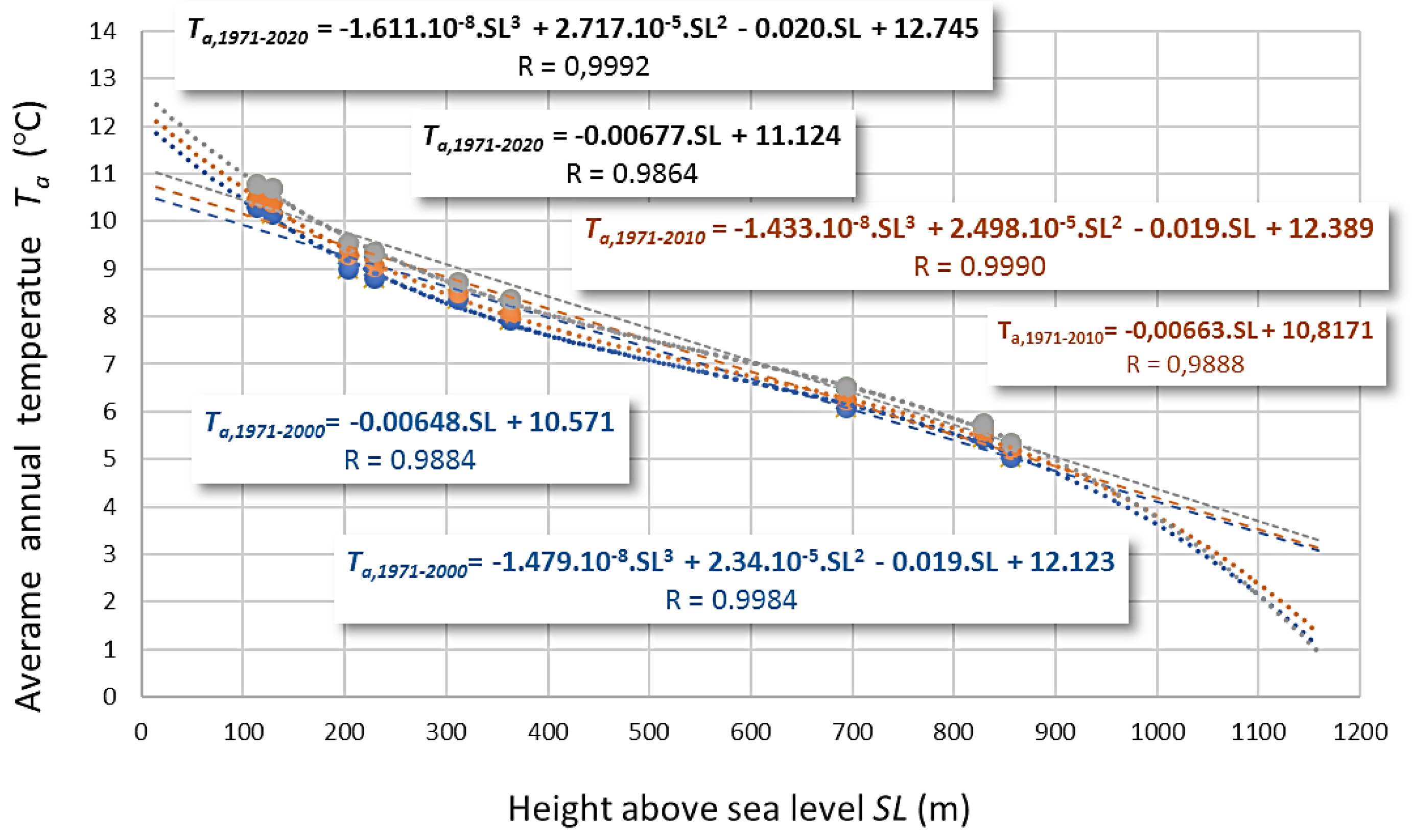
3.2. Correlation Dependencies of Average Annual Temperatures Ta on the Altitude of the Designed Pavement of Slovakia Evaluated for the Periods 1971–2000, 1971–2010, and 1971–2020

Figure 5 and Table 2 present the results of the author’s 20-year research in the field of prediction of the development of the average annual air temperature as one of the limiting factors in the assessment of cement concrete covers of rigid pavements. Table 2 presents the average annual temperatures of Ta for the periods 1971–2000, 1971–2010, and 1971–2020 and the increments of Ta between 2020 (2017) and 1971. It also presents overviews of the lowest average daily temperatures of the considered periods and an overview of the correlation coefficients from Figure 6.

4. Impact of Climate Change in Slovakia on Structural Design of CCP

4.1. Design Principles of CCP Design According to Slovak Road Act

There are three conventional types of cement-concrete pavements (CCP): jointed plain concrete pavements (JPCPs; Figure 7a,b), jointed reinforced concrete pavements (JRCPs; Figure 7c), and continuously reinforced concrete pavements (CRCPs; Figure 7d). All three common rigid pavements carry traffic loading through the flexural strength of the concrete. JPCPs are the most common type of rigid pavement due to their cost and simplicity in the United States of America [29,41], as well as in tunnel pavements in Slovakia [10]. Examples of the employment of JPCP in other countries—Moldova and Romania—are presented in [42,43].

Typically, a flexible (or asphalt) pavement is produced by continuously reducing the stiffness parameters of the individual layers to minimize stresses and deformations within the road body. The stiffest part of rigid pavements is the slab, under which layers with lower stiffness parameters can be applied. Furthermore, even when the stress in the rigid slab is increased, the overall deformation of the structure tends to decrease. The materials and thicknesses are chosen based on site-specific weather conditions.

Under CE conditions, the pavement is perceived as a paved part of the road intended for vehicles and consisting of a surface, a road foundation, and a capping layer. Cement-concrete pavement (CCP) represents a rigid pavement, i.e., a pavement substantially constructed of high-strength cement concrete [44]. The basis of the design of the CCP structure is the selection of materials for the layers of the base system, the design of the thickness of these layers, and the design of the dimensions of the CCS, their thickness, width, and length. The currently relevant regulations for the design of CCP is technical standard TP 098 [45], which specifies the procedure for designing, calculating, and assessing the structures of pavements with CC cover (wearing course) in Slovakia. The technical conditions for the design of CCP in the Slovak Republic, TP 098, are intended for investment organizations, designers, and construction organizations, as well as for the administration and maintenance of roads. The design of the structure, the choice of materials, as well as the criteria by which the dimensions of the pavements are assessed are differentiated according to the size of the traffic load and the type of cement-concrete cover.

The principles of designing roads with CCP in the Czech Republic are very similar to those in Slovakia. For the design of cement concrete coverings, the average annual air temperature is determined according to Annex A of ČSN 73 6114: 1995 [46]. This can be precisely determined from the data of meteorological stations in the given area for a mean return period of 10 years.

4.2. Assessment of Mechanical Efficiency of Cement Concrete Slab

According to Act No. 135/1961 Coll. on Roads (Road Act), the design of the pavement is carried out in accordance with valid Slovak technical standards, technical regulations, objectively determined results of research and development for road infrastructure, or similar technical specifications [44]. According to this act, the structural safety design of a CCS must satisfy condition (4). The limiting criterion is the assessment for a single load [45].

$$\frac{R_{i,n}}{{\sigma }_{\max ,OT}}=\frac{R_{i,n}}{{\sigma }_{DA,115kN}+{\sigma }_T}\ge {\xi }_i$$

(4)

Here, R_i,n (MPa) is the flexural tensile strength of the cement-concrete, σ_max,OT (MPa) is the maximum flexural tensile stress from a single load on the longitudinal or transverse joint of the CCS, σ_DA,115kN is the stress due to pure force load (design axle), and σ_T represents stress due to thermal load [45]. The safety ratio between its strength and its actual stress response is ξ_i. This value is necessary to establish when assessing a cement-concrete pavement (ξ_i > 1.10 for highways and ξ_i > 1.05 for Class 1 to III roads). The maximum flexural tensile stress σ_max,OT must be greater than or equal to the flexural tensile strength of the cement concrete R_i,n at the specified utilization factor.

Usually, the highest value of the maximum stress is achieved at the transverse or longitudinal joint of the CCS and therefore the correct design for these two load positions is assessed in Figure 8.

In the contraction joints and at the edge of the cement concrete slab, extreme normal stresses are expected. Therefore, the load is positioned at two critical points by the rear axle of the load vehicle. We consider one position in which the rear axle is most closely located to the intersection of the transverse and longitudinal contraction joints. It is always possible to consider the second position to be either the intersection of the transverse contraction joint or closest to the edge of the cement concrete slab. The current legislation requires the calculation to be conducted using the principles of FEM.

$${\sigma }_{T,x\left(y\right)}=\frac{E_{CC,T}\cdot \alpha \cdot \left(12.44-0.6\cdot T_a+28\cdot h_c\right)}{2}\cdot C_{x\left(y\right)}$$

(5)

The stresses from temperature change effects (σ_T,x(y) also TS _{temperature value}) can be solved using Equation (5). In this equation, E_CC,T is the modulus of elasticity for permanent load, $\alpha$ is the coefficient of thermal expansion, C_x(_y) (−) are the values of the coefficients (which are identified from Figure 9, according to TP 098 [45]), and h_c (m) is the critical design parameter-proposed slab thickness. Empirical value 12.44 is in °C and multiplication constant 28 has a physical dimension °C/m. The reduced modulus of elasticity of cement concrete is considered in the calculation of stresses induced by temperature loading. For longer time actions, this modulus of elasticity corresponds to its curing at E_CC,T = 27,500 (MPa) level. The coefficient of thermal expansion is α = 0.000012 (°C⁻¹).

$$l_T=\sqrt[4]{\frac{E_{CC,T}\cdot h_c^3}{12\cdot \left(1-{\nu }^2\right)\cdot k}}$$

(6)

Equation (6) determines the radius of relative stiffness under thermal stress l_T (m). ν is the Poisson’s constant, h_c (m) is the proposed slab thickness, E_CC,T is the modulus of elasticity for permanent load, and k is the modulus of reaction of the pavement system. The radius of relative stiffness under thermal stress l_T is an important value in the graph for the determination of the C_x (C_y) coefficient (Figure 9), the dimensions of the CCS L_x and L_y (m) and the Poisson’s constant ν = 0.2. The modulus of reaction of the pavement system k (MN·m⁻³) is recommended to be between 100 and 300 MN·m⁻³.

4.3. Determination of the Average Annual Air Temperature for the Calculation of Thermal Stresses

It is stated in TP 098 that the design of pavement with a cement-concrete cover must comply with the following: road protection against adverse effects of subgrade freezing, the ratio of concrete strength and tensile stress at bending in CCS due to one-time stress, the ratio of concrete flexural strength and tensile stress at bending in CCS due to repeated stress. Due to the great influence of temperature on deformation and stresses in CCSs (thermal stresses), it is always necessary to consider the combination of traffic load and the influence of the temperature regime of CCP in the calculations.

At the time of processing the submitted paper, to determine the average annual air temperature, together with the traffic loads of the decisive characteristics of the CCP assessment, STN 73 6114:1997 [40] was use, which contains the map presented in Figure 10.

For assessment, according to TP 098 [45], we must know the average annual air temperature T_a. Figure 11 shows the correlation dependences of the air temperatures of interest on the altitude SL of CCP found from 1971 to 2017 (2011). Specifically, the dependences include T_max—the maximum measured air temperature at 14 h for the period 1971–2011, T_{d, max}—the maximum average daily air temperature for the period 1971–2011, T_a,2021—the predicted average annual temperature in 2021 determined according to the equations in Figure 5, and T_{a, LLTZ}—the lower limit of the temperature zone determined from the map STN 736114: 1997 on the SL of the assessed pavement.

Figure 12 presents detailed results of sensitivity analyses of calculated thermal stress values for CCSs thicknesses of 12 to 32 cm and the modulus of the subgrade reaction values k = 100, 200, and 300 MN·m⁻³ determined by the procedure given in TP 098. The modulus of subgrade reaction k is used as a primary input for rigid pavement design. It estimates the support of the layers below a rigid pavement surface course (the PCCS). The k-value can be determined by field tests or by correlation with other tests. There is no direct laboratory procedure for determining the k-value. The modulus of subgrade reaction came about because work conducted by Westergaard during the 1920s led to the development of the k-value as a spring constant to model the support beneath the slab [24].

5. Calculation of the Response of a Real Cement Concrete Pavement in the Conditions of Slovakia

For the design and analysis of cement concrete pavements, there are a number of methods and processes currently available. In many developed countries around the world, numerical modelling is the most appropriate method. The finite element method (FEM) is one of the most effective general-purpose, numerical, variation methods for solving continuum mechanics boundary value problems. It is universal to the type, geometry, boundary conditions, and loading of the structure. The deformation variant is the most commonly used solution. Slovak legislation even requires pavements to be analyzed using FEM. Different types of FEM models are suitable for different application purposes, including the calculation of static and dynamic responses by means of their shapes, boundary conditions, types of finite elements, types of contacts, etc. By examining the analytical and experimental results that were presented, the FEM model is supposed to investigate the validity of its use in practice [47,48].

An example of a real pavement numerical analysis using FEM is presented in this section. Based on the above results of the sensitivity analysis of the calculated thermal stress values for CCSs with thicknesses from 12 to 32 cm, the thickness of the CCS was determined. This is approximately the average value in the range (19 cm). In this example, the temperature is not directly included in the stress calculation. By comparing both sections’ analyses, we can determine the influence of temperature. The CCS is the most important part of the model. In the model, only the contact stresses in the wheel tire on the slab surface are considered.

It has been determined which section of the roadway corresponds to the boundary conditions for the CC pavement thickness set out above. It has been selected as a plausible illustration of the use of numerical modelling in practice. This is the existing real section of the motorway near the town of Žilina, before the Ovčiarsko tunnel. In both sections, before and inside the tunnel, the proposed pavement composition is the same.

5.1. Solution Method and Numerical System

For this example, the IDA NEXIS system was used. It was chosen for its simplicity and user-friendliness. As a unique program, it overcomes barriers for ordinary users. For common purposes, its use is simple, natural, and intuitive and it provides diverse and rich features. The program uses the deformation variant of FEM to deal with 1D and 2D elements, plane strain, material and geometric nonlinearities, dynamics, stability analysis, and geotechnics. It is used to numerically analyze problems in civil engineering [49].

In this FEM system, the following steps are necessary in order to create a credible model:

• Stage 1 = Preprocessing—Preprocessing is performed for the preparation of the model-control using FEM. It includes the generation of the mesh, either surface or volume, and the following operations: automatic meshing, mesh crossing, operations (shifting, copying, mirroring, etc.), and mesh clipping. It defines the geometry of the finite element mesh, the individual boundary conditions, and the load.
• Stage 2 = Processing—The FEM equations are processed and solved. The system creates the equations and stiffness matrices using the data from the first stage automatically. This numerical procedure is automatically processed by a computer and does not require a user interface.
• Stage 3 = Postprocessing—Visualization and graphical display of the results of the entire analysis. These results can be presented numerically or as a video simulation.

The form of the feature function generally depends on the shape and type of the individual analysis [50]. Element convergence in FEM is also related to the element form characteristics of the function. This is very useful information for understanding heterogeneous shape functions and their properties. When developing a model, it is important to know when the elements of the structure interact with each other and when they behave as separate parts. This interaction can be identified for different variants of the model:

• Member-to-member interaction;
• Member interaction with plan elements (2D macros)—member point touching a plane element, member lying in a plane element;
• Interaction of planar elements (2D macros)—both modelled variants have a common edge, thus transferring all deformations and rotations.

For numerical pavement models, the interaction with the subgrade is most important. The soil-in module in NEXIS allows us to solve this type of problem. It includes the conversion of the geotechnical characteristics of the subgrade to stiffness C_i compressibility parameters. The calculation is performed on a nonlinear basis using iterations converging on the final response solution.

The module calculates the C_i parameters for the interaction between the foundation slab and the subgrade, considering the load distribution and intensity, the contact stress at the structure–soil interface, the foundation geometry, and the local geological conditions. The use of this module also offers other advantages such as multi-parametric interaction between the foundation slab and the subgrade, subgrade input using data obtained from exploratory boreholes, and others [51].

5.2. Numerical Calculation of Real CCP Structure in High Altitude

The location of this section ideally corresponds to the topic of the presented article. The Ovčiarsko tunnel, located on the D1 motorway in the section Hričovské Podhradie-Lietavská Lúčka, is a two-tube highway tunnel belonging to the medium-length tunnel category (2360 m). It forms part of the Žilina bypass. On motorways, due to their longer service life and lower maintenance costs, cement concrete pavements are designed and mechanically considered as thin slabs (Kirchhoff) with the elastic properties of reinforced or unreinforced concrete, which must satisfy the basic criteria for assessing the effects of cyclic loading by truck passes. As part of the design process, it is always advisable to assess the structural response of the various design options in terms of the structural layers [52].

5.2.1. Mechanical Characteristics of the Model

The main, stiffest part of the pavement structure of the model consists of a 190 mm-thick CB I cement concrete slab. This is followed by additional layers—40 mm thick AC 16 B asphalt concrete for the roadbed layer, under which is 180 mm thick CBGM C5/6 cementitious stabilization. The last 200 mm thick layer is ND gravel, under which the sub-base is placed. The total thickness of the modelled pavement is 610 mm. The composition of the structural layers and the summarized mechanical properties used for the modelled elements can be seen in

Table 3. Properties of CCP layers used for the numerical study.

Pavement Layer	Sign	Thickness	Mechanical Properties
			E (MPa)	ν (-)
Cement concrete cover-slab	CB I	190 mm	37,500	0.20
Asphalt concrete for roadbed	AC 16 B	40 mm	4200	0.30
Cement stabilization	CBGM C 5/6	180 mm	4500	0.22
Gravel crushed stone	ŠD	200 mm	350	0.30
Subbase	-	-	60	0.40

. The IDA NEXIS computational system allows the individual layers of the computational model to be modelled using the soil-in module, which allows the individual mechanical properties to be entered separately for each layer. The layer thicknesses are entered relative to the bottom edge of the cement concrete slab [53].

5.2.2. Considered Loads and Model Geometry

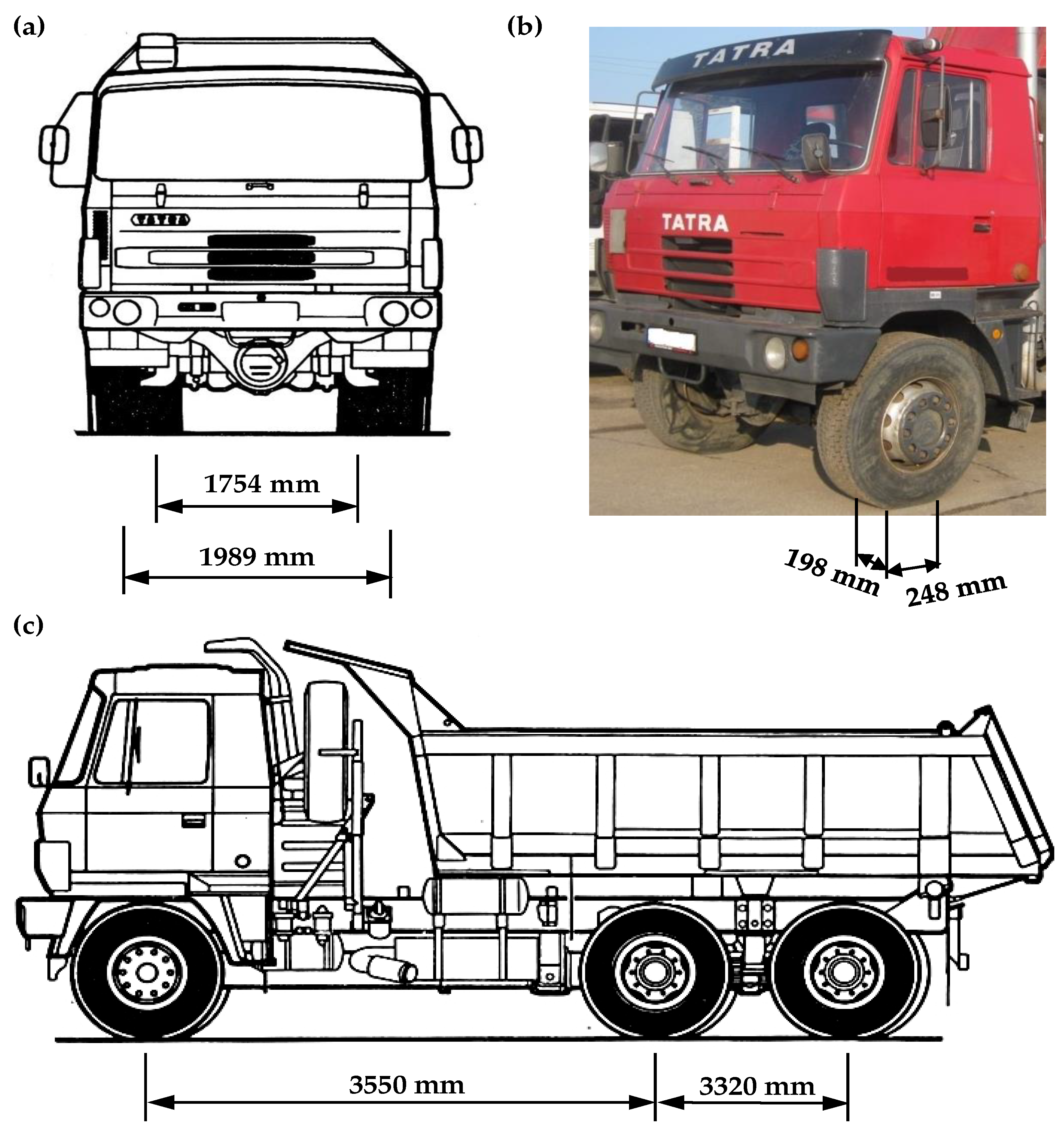
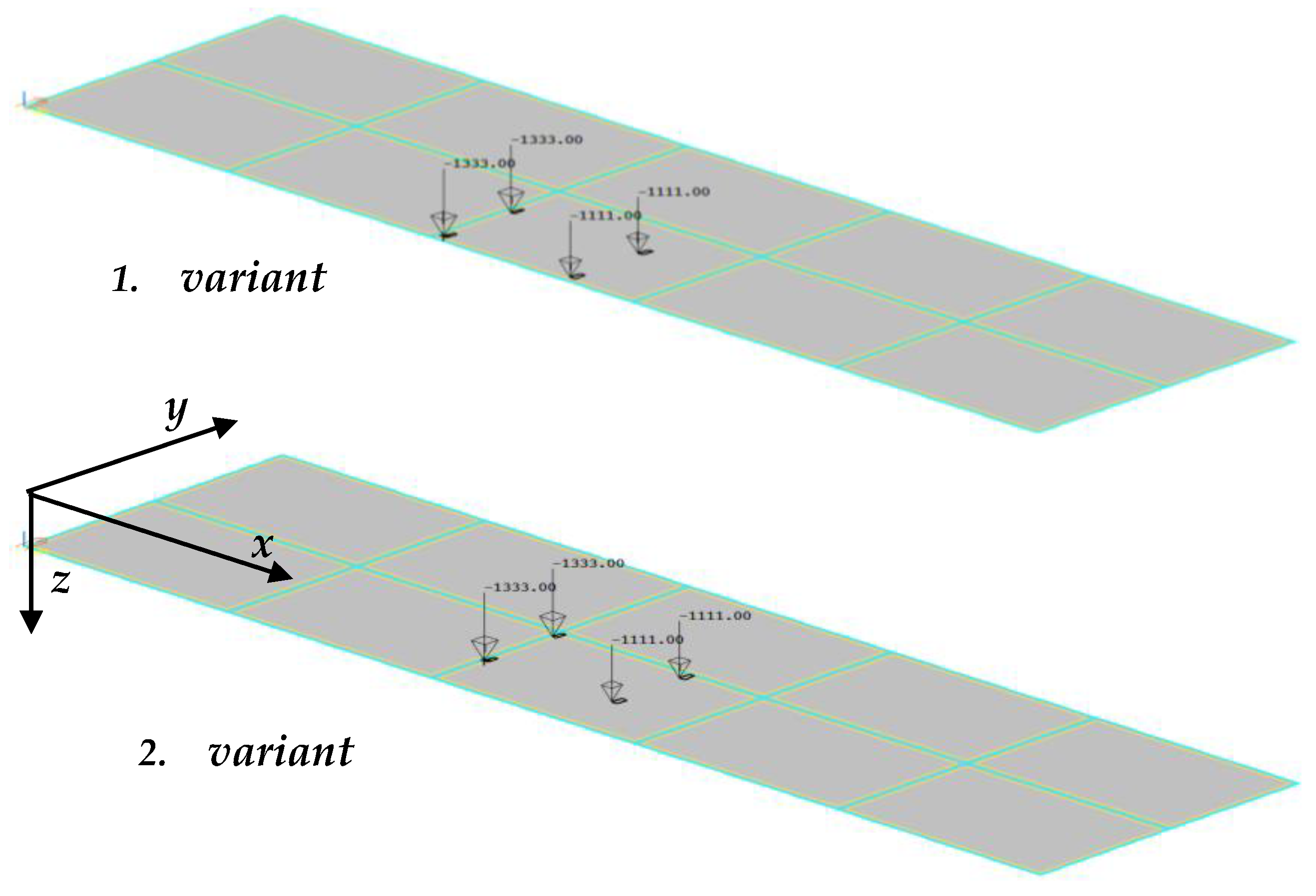
The numerical analysis considers the maximum realistic load, which is assessed using the basic criteria given in TP 098 [45]. The modelled pavement was loaded at the wheel pressure points of the front and rear axle of a TATRA T815-S3 26 208 truck [54]. This is a triple-folding truck, designed primarily for the transport of bulk materials up to 15,700 kg (Figure 13). The effect of the rear double axle is modelled as the wheel pressure of one rear axle in accordance with the regulation.

The most important parameters of the modelled load-vehicle needed for the model are:

• Axle distance 3550 mm;
• Distance between the wheels 1989 mm;
• Front axle load capacity 80 kN (8000 kg);
• Rear axle load 100 kN (10,000 kg).

Another important parameter in the modelling task is the contact area between the wheel and the road, which is in fact not an ideal rectangle but an idealized one. This area depends on several parameters. It is influenced by the weight exerted by the vehicle on the wheel, the speed of the moving vehicle, the pressure and type of tire used, the road roughness, the coefficient of friction, etc. Its determination is dealt with as concisely as possible in the literature [54]. This problem can also be solved by numerical simulations based on FEM. As an example, a computational model with the contact stress distribution of the tire-pavement in ABACUS is presented (Figure 13). For a standard vehicle tire width of 300 mm, a con-contact area length of 100 mm was considered for the front axle and 150 mm for the rear axle. The modelled highway section has a length of 5 × 6 m and a width of 2 × 4 m (contraction line continuous joints bordered). From the axle loads of each axle, the load on the contact patch in the vertical direction was expressed and then the load obtained was distributed evenly over the contact patch of the individual wheels. This is the wheel pressure in kN/m².

5.3. Results of Numerical Analysis of the CCP Highway Section Using FEM

The results of the numerical calculations are represented by the response of the pavement structure of the section in front of the tunnel to the above-specified static loads. This response can be divided into terms of stresses and strains. Both are then related to the assessment of the first and second limit states, as is generally the case for building structures. The results show two variants of the solution—Variant 1, loading at the outer edge of the modelled region and Variant 2, loading at the inner expansion (Figure 14).

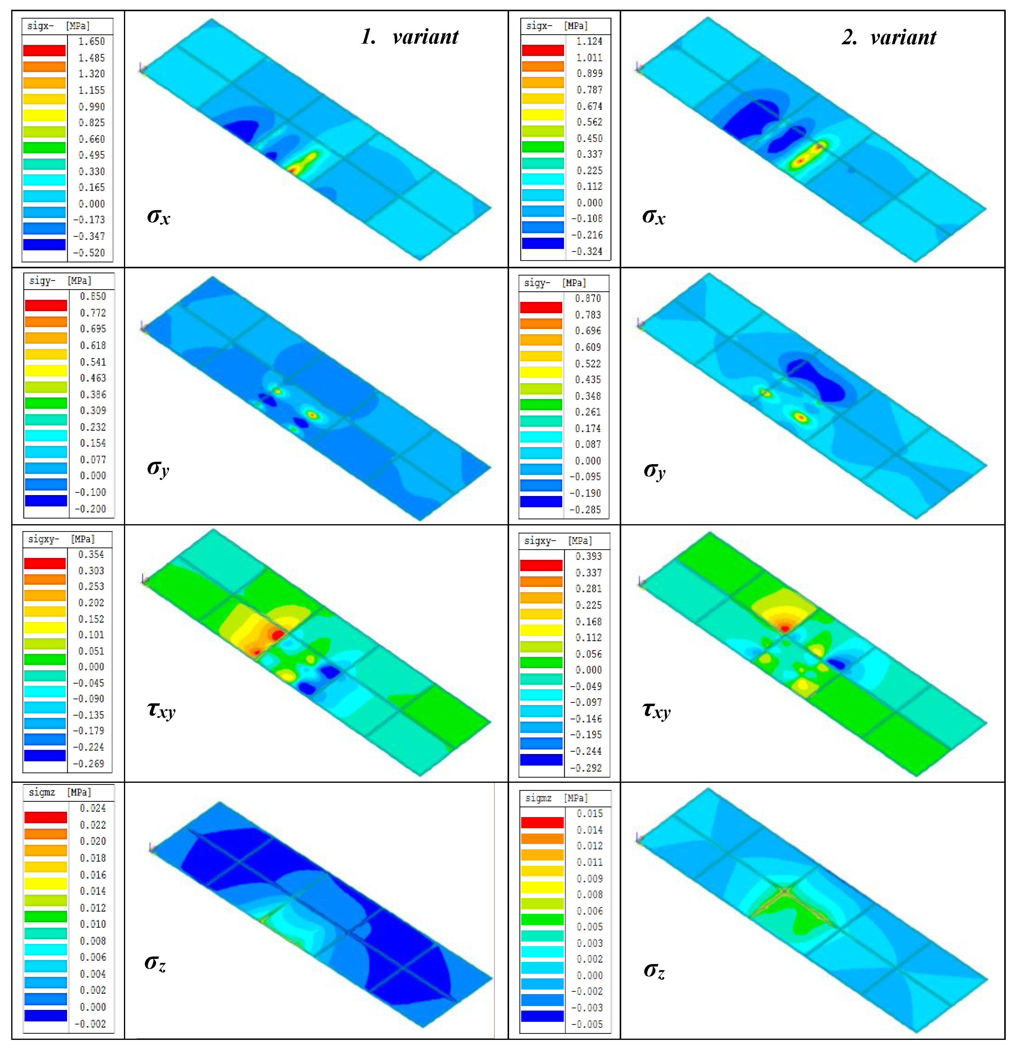
Since the CCP cover slab is the most important part of the model, only the contact stresses of the wheel tire on the slab surface are considered. Because they are assumed to be linear after the thickness of the slab (see elasticity theory). These stresses are represented along the median surface of the slab in the x-axis direction along the length—σ_x and the y-axis direction across—σ_y. Another surface stress is the stress τ_xy, which represents the shear stress in the horizontal plane. Figure 15 shows the waveforms of all three of these stresses σ_x, σ_y, and τ_xy for the variants considered, as well as the contact stresses between the CCP slab and the asphalt concrete for the surface layers σ_z.

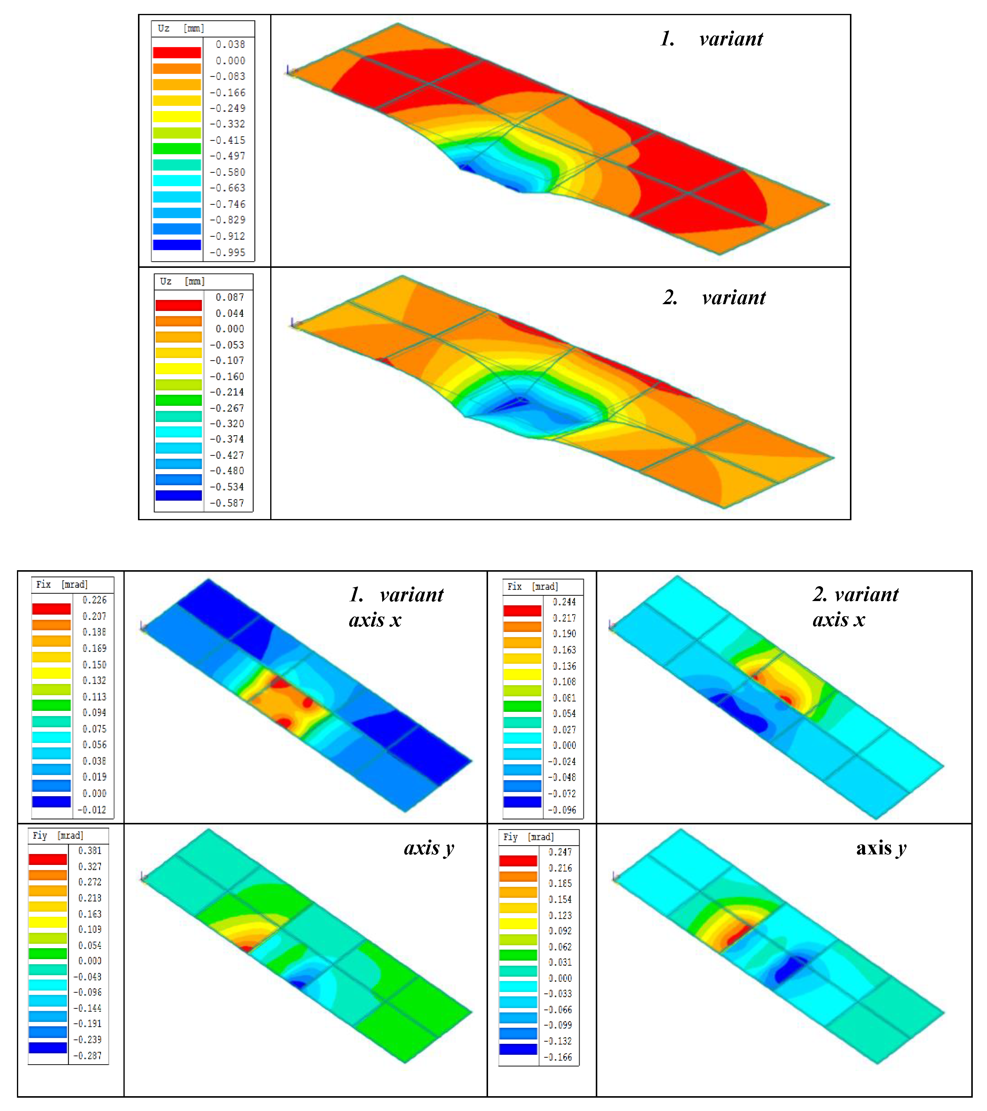
In terms of deformations, Figure 16 shows the vertical displacement or deflections of the slab and the rotations of the tangent surfaces. All outputs are in the form of isosurfaces. The color scale on the sides of the figures shows the maxima and minima of the individual values. The final table (

Table 4. Numerical results—maximal values and limit values according to standard TP 098.

Numerical Results	1. Variant	2. Variant
max σx	1.650 MPa	1.124 MPa
max σy	0.850 MPa	0.870 MPa
max τxy	0.354 MPa	0.393 MPa
max σz	0.024 MPa	0.015 MPa
max w	0.995 mm	0.587 mm
max φx	0.226 mrad	0.244 mrad
max φy	0.381 mrad	0.247 mrad
max σ1	1.652 MPa	1.124 MPa
min σ2	0.569 MPa	0.528 MPa
Criterial Limits
Flexural strength CB III	4.0 MPa	4.0 MPa
Limit deflection wlim	2.5 mm	2.5 mm

) summarizes the results of the static calculation using FEM.

The following partial conclusions are evident from both modelled options:

• Surface normal stresses σ_x—take their highest values on the underside of the slab in the axle area and gradually disappear at a distance of about 1 m from the axle. Values at greater distances are negligible. Their progression in the transverse direction is approximately constant between the wheels.
• Surface normal stresses σ_y—take on significant peaks directly at the contact surface of the wheels. Their values are the most pronounced and most influenced by the principal normal stresses. They decrease at very small distances and take negligible values.
• Surface shear stresses τ_xy—change sign between axles and also between wheels. They increase towards the force and decrease to zero when moving away from the force. Their values are the least significant.
• Centre-plane deflections—it is evident from the deflections that the largest deflections are directly under the wheels of the vehicle. The values gradually decrease in the transverse direction between the wheels and also in the longitudinal direction between the axles. They disappear approximately 1 m in front and 1 m behind the vehicle.
• Rotations of the tangent surfaces—about the x, y axes, these values are related to the deflections and the deflection surface. They correspond to deflections because they are their first derivative.

The various load designs for the pavements show minimal differences in the individual design values of the mechanical quantities of interest, suggesting that the difference in the composition of the pavement structural layers in question does not have a significant effect on the governing stresses. The strength characteristics and deflection limit values are not exceeded.

6. Discussion

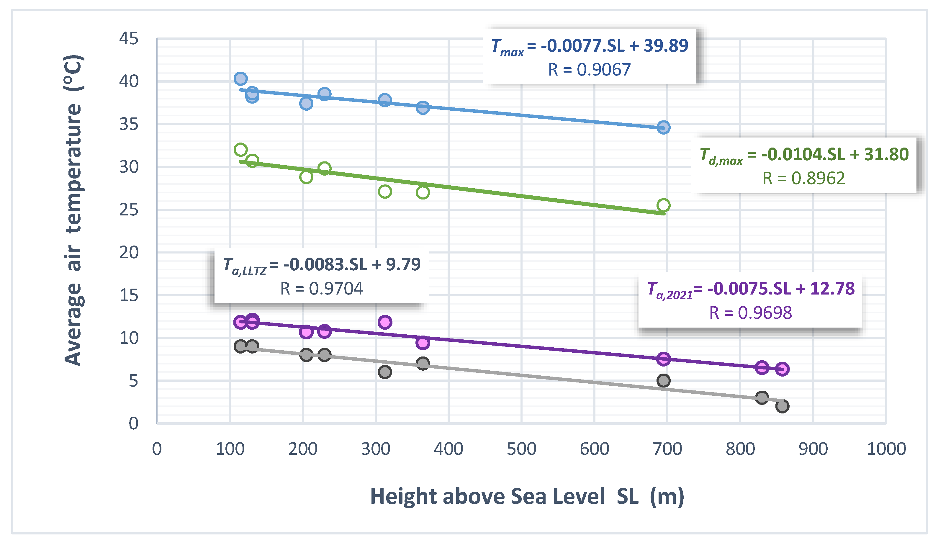
The authors present the results of 25 years of research in the field of adaptability of transport structures, especially road pavements, to climate change in Slovakia, located in CE. Based on the analysis of the development and current state of perception of Central Europe, for the purposes of this article, they defined its schematic territory according to Figure 4. The article presents a linear and polynomic correlation dependence of average annual temperature T_a (°C) on the SL altitude above sea level (m) of the designed pavements of Slovakia evaluated for the periods 1971–2000, 1971–2010, and 1971–2020. For technical practice purposes, we recommend using the following equation determined from the period 1971 to 2020 (Figure 11).

$$T_{a,1971-2020}=-0.0067\times SL+11.24$$

(7)

The average annual temperatures of 10.6 to 3.8 °C correspond to the determined range of altitudes inhabited by the Central European territories of 100 to 1100 m. For the purposes of judging Central European road pavements, the following dependencies were specifically used (

Table 5. Correlation dependences of average annual temperature T_a (°C), average daily temperature T_d (°C), and the maximum air temperature T_max (°C) determined from the highest measured temperatures in CS on the SL (m) of pavement and the average increase in T_a climate stations (CS) between 2020 and 1971.

Correlation Dependences of Average Ta (°C) and Maximal Tmax (°C) Temperatures on the Height above Sea Level SL (m)		T (°C) of Permanently Inhabited Settlements in Central Europe Calculated According to Equations (7)–(10) for the Altitude SL (m)
		100 m	1100 m	Difference T100–T1100
$T_{\max }=-0.0077\times SL+39.89$  (7)		38.1	30.4	7.7
$T_{d,\max }=-0.0104\times SL+31.80$ (8)		30.8	20.4	10.4
$T_{a,2021}=-0.0075\times SL+12.78$ (9)		12.0	4.5	7.5
$T_{a,LLTZ}=-0.0083\times SL+9.79$ (10)		9.0	0.7	8.3
Average increase of Ta climate stations (CS) for the period (Figure 5)	Period	Average of All 10 CS	CS on the Airports	Others CS
	1971 to 2020	2.1	2.7	1.9
	1976 to 2006	1.3	1.6	1.2

):

• T_max—the maximum measured air temperature at 14 h for the period 1971–2011 (°C);
• T_d,max—the maximum average daily air temperature for the period 1971–2011 (°C);
• T_a,2021—the predicted average annual temperature in 2021 determined according to the equations in Figure 3 (°C);
• T_a,LLTZ—the lower limit of the temperature zone determined from the map STN 736114: 1997 (°C) on the height above sea level SL (m) of designed pavements.

It is clear from Table 5 that climatic stations (CS) at airports show a significantly higher increase in T_a (2.7°) than other CS (1.9°), which is probably caused by large areas of asphalt or cement-concrete pavements. Between 1971 and 2020, an average increase in T_a of 2.1 °C was found in Slovakia, which is about 0.7 °C higher (Figure 1) than the average increase reported by the Intergovernmental Panel on Climate Change (IPCC). By comparing the research results presented in this paper and [7,46] with the findings of the European Environment Agency from 1976 to 2006 (Figure 2), full compatibility of the outputs was identified. For the period 1976 to 2006, the EEA presents an average increase T_a in Central Europe of 1.2 to 1.5 ° C and the authors found a value of 1.3 ° C in Slovakia (Table 5).

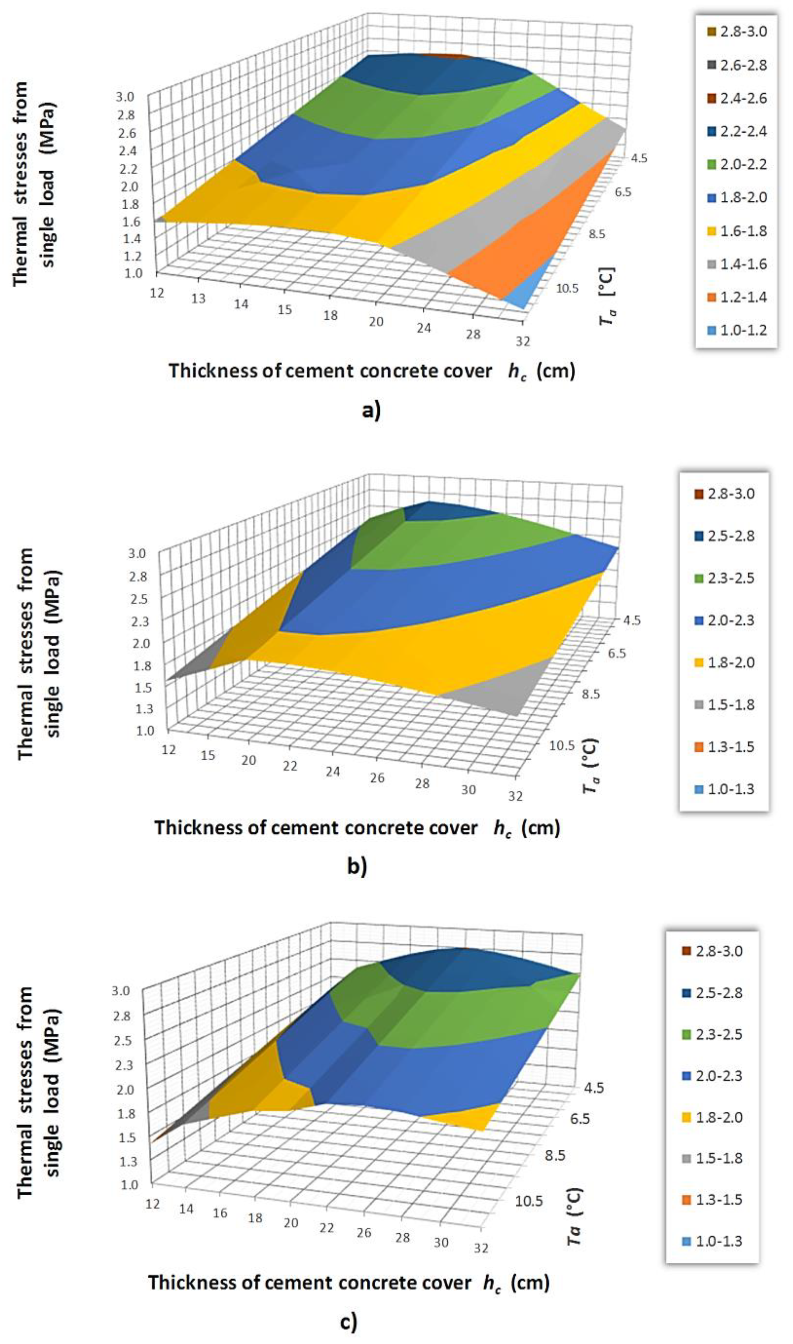
The accuracy of the CCP design is currently limited in Slovakia due to the accuracy of the determination of T_a, since the effects of traffic load can be calculated with high accuracy by means of FEM (Section 5). The important conclusion is Figure 11, where the authors present the dependences of thermal stresses from a single load of 115 kN designed for thicknesses from 12 to 32 cm of cement-concrete cover h_c on the annual average air temperature T_a from 4.5 to 11.5 °C for the modulus of subgrade reaction k = 100, 200, and 300 MN·m⁻³ [55].

To illustrate the significant effect of T_a on thermal stresses (TS), we give corresponding numerical values for h_c = 20 cm and dimensions of CCSs 4 × 4 m. The summarized results are shown in

Table 6. The summarized results.

Modulus of Subgrade Reaction k	Thermal Stresses for Air Temperature 4.5 °C		Thermal Stresses for Air Temperature 11.5 °C
k = 100 MN·m−3	TS4.5 = 2.26 MPa		TS11.5 = 1.64 MPa
k = 200 MN·m−3	TS4.5 = 2.63 MPa		TS11.5 = 1.91 MPa
k = 300 MN·m−3	TS4.5 = 2.72 MPa		TS11.5 = 1.92 MPa
Numerical Results—Surface Normal and Shear Stresses
1. Variant		2. Variant
σx = 1.650 MPa		σx = 1.124 MPa
σy = 0.850 MPa		σy = 0.870 MPa
τxy = 0.354 MPa		τxy = 0.393 MPa

(TS_Ta=4.5 = TS_4.5).

The above results indicate that the analytical solution for the stress profile of the standard load and the actual temperature load from the focus research part of the paper is valid. Surface maximum stress values of normal stresses obtained by FEM calculation represent 61% to 82% of all maximum stress values obtained by analytical calculation. Due to this, it is evident that reinforced concrete slabs are the most effective structure regardless of the stiffness of the subgrade. This type of road body structure is less vulnerable to the effect of temperature variations.

Based on the above research results, it can be stated that the current climatic characteristics used for pavement design in Slovakia do not take into account current climate change. The authors are fully aware of the serious negative effects of climate change on pavement structures, but these changes have a positive effect on the structural design. Global warming causes a significant increase in T_a, which allows for the structural design of road pavements with lower overall thicknesses, as well as h_c in the case of cement-concrete pavements (CCP) [56].

In Central Europe, more attention has been paid in the last 10 years to the development of innovative climate-adaptable asphalt mixture, [57,58,59,60], as well as cement-bound granular mixtures [60,61]. In all presented innovative materials [57,58,59,60,61] temperatures play a significant role in both the mix design and structure design of pavements. For this reason, we actually focus on the implementation of the presented knowledge to the development of composite foam concrete for the base layers of civil engineering structures [62].

7. Conclusions

The results of temperature change monitoring presented in the substantive sections of this paper are relevant to studies dealing with the effect of temperature change on stress increase in CCS [63,64,65], which are presented in world-renowned and highly cited publications. In terms of conclusions, the results need to be divided into the time-lapse original data, the mathematical analysis, the correlation and approximation of dependencies that led to the predictive models, the numerical–analytical solution of the response to force, and temperature effects of the load. In these results and their detailed analysis, it is possible to find a solution for the specific participation of stress effects in the computational models of this part of the pavement structure. Since this is a structural part that is exposed to weather effects and is also directly impacted by traffic loads, one of the main conclusions is the directly specified proportion of temperature and force loads. We can see a few differences between the standard solution of the stress response presented in the literature [66,67,68] and the findings presented in Section 3, Section 4, and Section 5 of the paper. Taking these comparisons into account, it can be concluded that CE should be considered a specific area, especially when it comes to some of the regions mentioned in Section 2 (in Slovakia). In this context, it is a more sensitive approach to assessing stresses that arise in CCP. In addition, it is also important to define the necessity to modify standards and regulations to take into account location-related phenomena. Another interesting conclusion relates to the potential for creating a predictive mathematical model based on correlations of results between the long-term monitoring of temperature changes (years 1971 to 2020). Further implementation of the model can be undertaken to assess the suitability of CCP use or to define more precisely the impact of temperature on design over a longer time horizon.

The contributions of the paper must be restricted to the scientific community in Central Europe engaged in road construction research. The long-term monitoring of temperature changes in Slovakia has produced significant original results. Throughout the territory of CE, the variability of mountain ranges and plains is affected in different ways by global climate change. This is a characteristic of Slovakia. The results reported in the experimental sections of the paper will be used to conduct research on advanced materials and additives for cement-concrete pavements. One of the main conclusions is that their use is most appropriate in terms of mitigating the effects of temperature on CCPs.

The results of the measurements can also influence the CCP design methodology to introduce mandatory monitoring and diagnostics of pavement structures for specified territories most significantly impacted by temperature changes.

References

1. Qin, Y. A review on the development of cool pavements to mitigate urban heat island effect. Renew. Sustain. Energy Rev. 2015, 52, 445–459. [Google Scholar] [CrossRef]
2. Yaghoobian, N.; Kleissl, J. An indoor–outdoor building energy simulator to study urban modification effects on building energy use—Model description and validation. Energy Build. 2012, 54, 407–417. [Google Scholar] [CrossRef]
3. Change, I.C. The Physical Science Basis: Contribution of Working Group I to the Fourth Assessment Report of the Intergovernmental Panel on Climate Change; Cambridge University Press: Cambridge, UK, 2007; p. 996. [Google Scholar]
4. Pachauri, R.K.; Allen, M.R.; Barros, V.R.; Cramer, W.; Christ, R.; Church, J.A.; Clarke, L.; Dahe, Q.; Dasgupta, P. Climate Change 2014: Synthesis Report. Contribution of Working Groups I, II and III to the Fifth Assessment Report of the Intergovernmental Panel on Climate Change; IPCC: Geneva, Switzerland, 2014; p. 151. [Google Scholar]
5. Shukla, P.R.; Skea, J.; Buendia, E.C.; Masson-Delmotte, V.; Portner, H.-O.; Roberts, D.C.; Zhai, P.; Slade, R.; Connors, S.; Diemen, V.; et al. Climate Change and Land: An IPCC Special Report on Climate Change, Desertification, Land Degradation, Sustainable Land Management, Food Security, and Greenhouse Gas Fluxes in Terrestrial Ecosystems; IPCC: Geneva, Switzerland, 2019; Available online: www.ipcc.ch (accessed on 20 December 2021).
6. Observed Temperature Change over Europe 1976–2006. Available online: https://www.eea.europa.eu/data-and-maps/figures/observed-temperature-change-over-europe-1976-2006 (accessed on 26 December 2021).
7. Hodakova, D.; Zuzulova, A.; Capayova, S.; Schlosser, T. Impact of climate characteristics on cement concrete pavements. In Proceedings of the International Multidisciplinary Scientific GeoConference: SGEM, Sofia, Bulgaria, 29 June–5 July 2017; Volume 17, pp. 467–472. [Google Scholar] [CrossRef]
8. Hodáková, D.; Zuzulová, A.; Cápayová, S.; Schlosser, T. Temperature changes as decisive loads on cement concrete pavements. In Proceedings of the International Multidisciplinary Scientific GeoConference: SGEM, Sofia, Bulgaria, 30 June–6 July 2019; Volume 19, pp. 1093–1100. [Google Scholar]
9. Domonkos, P.; Kyselý, J.; Piotrowicz, K.; Petrovic, P.; Likso, T. Variability of extreme temperature events in south-central Europe during the 20th century and its relationship with large-scale circulation. Int. J. Clim. 2003, 23, 987–1010. [Google Scholar] [CrossRef]
10. Decky, M.; Juhas, M. Impact of climatic characteristics on dimensioning of road construction in tunnels in Slovakia. In Proceedings of the International Multidisciplinary Scientific GeoConference SGEM, Albena, Bulgaria, 16–22 June 2013; p. 659. [Google Scholar]
11. Trojanová, M.; Decký, M.; Remišová, E. The Implication of Climatic Changes to Asphalt Pavement Design. Procedia Eng. 2015, 111, 770–776. [Google Scholar] [CrossRef] [Green Version]
12. Sinnhuber, K.A. Central Europe: Mitteleuropa: Europe Centrale: An Analysis of a Geographical Term. Trans. Pap. (Inst. Br. Geogr.) 1954, 20, 15–39. [Google Scholar] [CrossRef]
13. Pynsent, R.B. Tinkering with the Ferkos: A kind of slovakness. Slavon. East Eur. Rev. 1998, 76, 279–295. [Google Scholar]
14. Petritsch, W. Culture in Central Europe: Possibilities and Preconditions. Anal. Cent. East. Eur. Rev. Engl. Ed. 2008, 1, 131–140. [Google Scholar]
15. Central Intelligence Agency (CIA). The World Factbook; Pentagon Publishing: Snellville, GA, USA, 2011; (accessed on 26 December 2021). [Google Scholar]
16. Available online: https://en.wikipedia.org/wiki/Geographical_midpoint_of_Europe (accessed on 20 December 2021).
17. Dobrovolný, P.; Moberg, A.; Brázdil, R.; Pfister, C.; Glaser, R.; Wilson, R.; Van Engelen, A.; Limanówka, D.; Kiss, A.; Halíčková, M.; et al. Monthly, seasonal and annual temperature reconstructions for Central Europe derived from documentary evidence and instrumental records since AD 1500. Clim. Chang. 2009, 101, 69–107. [Google Scholar] [CrossRef]
18. Available online: https://www.climate.gov/news-features/understanding-climate/climate-change-global-temperature (accessed on 15 March 2022).
19. Dong, D.; Huang, G.; Qu, X.; Tao, W.; Fan, G. Temperature trend–altitude relationship in China during 1963–2012. Theor. Appl. Climatol. 2015, 122, 285–294. [Google Scholar]
20. Available online: https://www.ipcc.ch/sr15/chapter/chapter-1 (accessed on 20 December 2021).
21. Basha, G.; Kishore, P.; Ratnam, M.V.; Jayaraman, A.; Kouchak, A.A.; Ouarda, T.B.M.J.; Velicogna, I. Historical and Projected Surface Temperature over India during the 20th and 21st century. Sci. Rep. 2017, 7, 2987. [Google Scholar] [CrossRef] [Green Version]
22. Dimitrov, R.S. The Paris Agreement on Climate Change: Behind Closed Doors. Glob. Environ. Politics 2016, 16, 1–11. [Google Scholar] [CrossRef] [Green Version]
23. Rogelj, J.; Popp, A.; Calvin, K.V.; Luderer, G.; Emmerling, J.; Gernaat, D.; Fujimori, S.; Strefler, J.; Hasegawa, T.; Marangoni, G.; et al. Scenarios towards limiting global mean temperature increase below 1.5 °C. Nat. Clim. Chang. 2018, 8, 325–332. [Google Scholar] [CrossRef]
24. Mikhailenko, P.; Piao, Z.; Kakar, M.R.; Bueno, M.; Athari, S.; Pieren, R.; Heutschi, K.; Poulikakos, L. Low-Noise pavement technologies and evaluation techniques: A literature review. Int. J. Pavement Eng. 2020, 20, 1–24. [Google Scholar] [CrossRef]
25. Decky, M.; Scherfel, W.; Remisova, E. Sustainable Materials and Technologies for Pavement Construction and Strengthening of Transport Areas; University textbook; University of Zilina: Zilina, Slovakia, 2021; p. 326. (In Slovak) [Google Scholar]
26. Mikolaj, J.; Remek, L.; Kozel, M. Optimization of Life Cycle Extension of Asphalt Concrete Mixtures in regard to Material Properties, Structural Design, and Economic Implications. Adv. Mater. Sci. Eng. 2016, 2016, 6158432. [Google Scholar] [CrossRef] [Green Version]
27. Colglazier, W. Sustainable development agenda: 2030. Science 2015, 349, 1048–1050. [Google Scholar] [CrossRef]
28. Schindler, A.K.; McCullough, B.F. Importance of Concrete Temperature Control During Concrete Pavement Construction in Hot Weather Conditions. Transp. Res. Rec. J. Transp. Res. Board 2002, 1813, 3–10. [Google Scholar] [CrossRef]
29. Delatte, N.J. Concrete Pavements Design, Construction and Performance, 2rd ed; CRC Press Taylor & Francis Group: Boca Raton, FL, USA, 2017; p. 421. ISBN 13:978-1-138-07354-8. [Google Scholar]
30. Richardson, J.M.; Armaghani, J.M. Stress Caused by Temperature Gradient in Portland Cement Concrete Pavements; Transportation Research Board, Washington District of Columbia, United States, No. 1121; Transportation Research Board: Washington, DC, USA, 1987. [Google Scholar]
31. The World Factbook: Field Listing—Location; The World Factbook; Central Intelligence Agency: McLean, VA, USA, 2009.
32. Zar, J.H. Significance testing of the Spearman rank correlation coefficient. J. Am. Stat. Assoc. 1972, 67, 578–580. [Google Scholar] [CrossRef]
33. Sedgwick, P. Spearman’s rank correlation coefficient. BMJ 2014, 349, g7327. [Google Scholar] [CrossRef] [PubMed] [Green Version]
34. Zhang, W.-Y.; Wei, Z.-W.; Wang, B.-H.; Han, X.-P. Measuring mixing patterns in complex networks by Spearman rank correlation coefficient. Phys. A Stat. Mech. Its Appl. 2016, 451, 440–450. [Google Scholar] [CrossRef]
35. Pearson, K. VII. Note on regression and inheritance in the case of two parents. Proc. R. Soc. Lond. 1895, 58, 240–242. [Google Scholar]
36. Galton, F. Regression towards mediocrity in hereditary stature. J. Anthropol. Inst. Great Br. Irel. 1886, 15, 246–263. [Google Scholar] [CrossRef]
37. Bravais, A. Analyse Mathématique sur les Probabilités des Erreurs de Situation d’un Point; Imprimerie Royale: Paris, France, 1844. [Google Scholar]
38. Hinkle, D.E.; Wiersma, W.; Jurs, S.G. Applied Statistics for the Behavioral Sciences; Houghton Mifflin College Division: Boston, MA, USA, 2003; Volume 663. [Google Scholar]
39. Spearman’s Correlation. Available online: http://www.statstutor.ac.uk/resources/uploaded/spearmans.pdf (accessed on 20 January 2019).
40. STN 73 6114; Pavement of Roads. Basic Provision for Structural Design. Slovak Standard; Slovak Office of Standards, Metrology and Testing: Bratislava, Slovakia, 1997. (In Slovak)
41. Mallick, R.B.; El-Korchi, T. Pavement Engineering: Principles and Practise, 3rd ed; CRC Press by Taylor &Francis Group: Abingdon, UK, 2018; p. 747. ISBN 978-3-4987-5880-2. [Google Scholar]
42. Pérez-Acebo, H.; Mindra, N.; Railean, A.; Rojí, E. Rigid pavement performance models by means of Markov Chains with half-year step time. Int. J. Pavement Eng. 2019, 20, 830–843. [Google Scholar] [CrossRef]
43. Pleșcan, C.; Pleșcan, E.-L.; Stanciu, M.D.; Botiș, M.; Taus, D. Sensitivity Analysis of Rigid Pavement Design Based on Semi-Empirical Methods: Romanian Case Study. Symmetry 2021, 13, 168. [Google Scholar] [CrossRef]
44. Act no. 135/1961, Act on Roads (Road Law), Slovak Government, Bratislava, Slovakia, 1961, Coll. on Roads (Road Act). Available online: https://www.slov-lex.sk/pravne-predpisy/SK/ZZ/1961/135/vyhlasene_znenie.html (accessed on 1 June 2021).
45. Zuzulova, A. TP 098 Cement Concrete Pavement Design on Road Network; Technological Standard of Ministry of Transport; Construction and Regional Development of the Slovak Republic, Section for Road Transport and Roads, Slovak road administration: Bratislava, Slovakia, 2015. [Google Scholar]
46. CSN 73 6114; Road Pavements. Basic Requirementsfor Design, Slovak Standard; Slovak Office of Standards, Metrology and Testing: Bratislava, Slovakia, 1995. (In Czech)
47. Kadela, M. Model of multiple-layer pavement structure-subsoil system. Bull. Pol. Acad. Sci. Tech. Sci. 2016, 64, 751–762. [Google Scholar] [CrossRef] [Green Version]
48. Gu, H.; Jiang, X.; Li, Z.; Yao, K.; Qiu, Y. Comparisons of Two Typical Specialized Finite Element Programs for Mechanical Analysis of Cement Concrete Pavement. Math. Probl. Eng. 2019, 2019, 9178626. [Google Scholar] [CrossRef]
49. Fricova, J. Effects of Technical Seismicity Induced by Road Traffic on the Historical Building of the Church of St. Stephen the King in Modra. Master’s thesis, UNIZA, Žilina, Slovakia, 2015. [Google Scholar]
50. Papanova, Z. Dynamic Soil-Foundation Interaction in Engineering Seismicity. Ph.D. Thesis, UNIZA, Žilina, Slovakia, 2013. [Google Scholar]
51. Papan, D. The forklifts groung vibrations effects on the sensitive machines. In Proceedings of the GEOconference on science and technologies in geology, exploration and 14th international multidisciplinary scientific geoconference SGEM, Albena, Bulgaria, 10 March 2014; pp. 17–26. [Google Scholar]
52. Papán, D.; Demeterová, K. The Dynamic FEM Models Results Comparison of the New Bridge over Danube River in Bratislava. Procedia Eng. 2016, 161, 1300–1307. [Google Scholar] [CrossRef] [Green Version]
53. Kuchárová, D.; Lajčáková, G. Modelling of moving load effect on concrete pavements. MATEC Web Conf. 2017, 107, 00025. [Google Scholar] [CrossRef] [Green Version]
54. Available online: www.valka.cz/CZK-Tatra-815-S3-26-208-6x6-2-t16298 (accessed on 27 December 2021).
55. Behroozinia, P.; Khaleghian, S.; Taheri, S.; Mirzaeifar, R. An investigation towards intelligent tyres using finite element analysis. Int. J. Pavement Eng. 2018, 21, 311–321. [Google Scholar] [CrossRef]
56. Šrámek, J. Stiffness and Fatigue of Asphalt Mixtures for Pavement Construction. Slovak J. Civ. Eng. 2018, 26, 24–29. [Google Scholar] [CrossRef] [Green Version]
57. Chomicz-Kowalska, A.; Maciejewski, K.; Iwański, M.M. Study of the Simultaneous Utilization of Mechanical Water Foaming and Zeolites and Their Effects on the Properties of Warm Mix Asphalt Concrete. Materials 2020, 13, 357. [Google Scholar] [CrossRef] [Green Version]
58. Iwański, M.M.; Chomicz-Kowalska, A.; Maciejewski, K. Resistance to Moisture-Induced Damage of Half-Warm-Mix Asphalt Concrete with Foamed Bitumen. Materials 2020, 13, 654. [Google Scholar] [CrossRef] [Green Version]
59. Remišová, E.; Holešová, N.; Brna, M. Influence of mineral aggregate on asphalt pavement surface properties. IOP Conf. Ser. Mater. Sci. Eng. 2021, 1015, 012072. [Google Scholar] [CrossRef]
60. Decký, M.; Drusa, M.; Zgútová, K.; Blaško, M.; Hájek, M.; Scherfel, W. Foam Concrete as New Material in Road Constructions. Procedia Eng. 2016, 161, 428–433. [Google Scholar] [CrossRef] [Green Version]
61. Vlcek, J.; Drusa, M.; Scherfel, W.; Sedlar, B. Experimental Investigation of Properties of Foam Concrete for Industrial Floors in Testing Field. IOP Conf. Ser. Earth Environ. Sci. 2017, 95, 022049. [Google Scholar] [CrossRef] [Green Version]
62. Kadela, M.; Kukiełka, A.; Małek, M. Characteristics of Lightweight Concrete Based on a Synthetic Polymer Foaming Agent. Materials 2020, 13, 4979. [Google Scholar] [CrossRef]
63. Małek, M.; Jackowski, M.; Łasica, W.; Kadela, M. Influence of Polypropylene, Glass and Steel Fiber on the Thermal Properties of Concrete. Materials 2021, 14, 1888. [Google Scholar] [CrossRef]
64. Mackiewicz, P.; Szydło, A. Thermal Stress Analysis in Concrete Pavements. J. Transp. Eng. Part B Pavements 2020, 146, 06020002. [Google Scholar] [CrossRef]
65. Wistuba, M.P.; Walther, A. Consideration of climate change in the mechanistic pavement design. Road Mater. Pavement Des. 2013, 14, 227–241. [Google Scholar] [CrossRef]
66. Mackiewicz, P. Thermal stress analysis of jointed plane in concrete pavements. Appl. Therm. Eng. 2014, 73, 1169–1176. [Google Scholar] [CrossRef]
67. Pereira, P.; Pais, J. Main flexible pavement and mix design methods in Europe and challenges for the development of an European method. J. Traffic Transp. Eng. (Engl. Ed.) 2017, 4, 316–346. [Google Scholar] [CrossRef] [Green Version]
68. Islam, M.R.; Tarefder, R.A. Pavement Design: Materials, Analysis, and Highways; McGraw-Hill Education: New York, NY, USA, 2020. [Google Scholar]
Figure 1. According to the Intergovernmental Panel on Climate Change (IPCC), since the pre-industrial period (1850–1900), the observed mean land surface air temperature has risen considerably more than the global mean surface (land and ocean) temperature.
Land 11 00764 g001
Figure 2. Observed temperature change over Europe during the period 1976–2006 according to the European Environment Agency. Reprinted with permission from [6]. Copyright 2021 by the European Environment Agency.
Land 11 00764 g002
Figure 3. (a) Middle Europe as a positional, historical, political, cultural and geographical concept: a graded assessment of the degree of coincidence existing between sixteen definitions of Middle Europe, 1954. Reprinted with permission from [12]. Copyright 1999–2022 by the Wiley Online Library. (b) Central Europe according to The World Factbook, Encyclopedia Britannica, and Brockhaus Enzyklopädie [15].
Land 11 00764 g003
Figure 4. On the map [16], the red dots indicate some of the places where claimants for the title of the center of Europe are located: Dilove (Rakhiv, Ukraine), Krahule (or Kremnické Bane, Slovakia), Dresden and Kleinmaischeid (Germany), Torun and Suchowola (Poland), Bernotai or Purnuskes (Lithuania). Schematic representation by the authors of the article of the considered Central European area is highlighted by a blue ellipse. Reprinted with permission from [16]. Copyright 2009 by the Creative Commons.
Land 11 00764 g004
Figure 5. Development of the average annual air temperature of 10 climatological stations in Slovakia at an altitude of 115 to 858 meters above sea level for the period 1971 to 2020.
Land 11 00764 g005
Figure 6. Linear and polynomic correlation dependences of average annual temperatures Ta on the altitude of the designed pavement evaluated for the periods of 1971–2000, 1971–2010, and 1971–2020.
Land 11 00764 g006
Figure 7. Jointed plain concrete pavement (JPCP) with tiebars and (a) no dowels and (b) with dowels, (c) jointed reinforced concrete pavements with tiebars and dowels, (d) continuously reinforced concrete pavements (CRCP). The figure was adapted from [41].
Land 11 00764 g007
Figure 8. Design process of CCP according to TP 098. Reprinted with permission from [45]. Copyright 2022 by the Slovak Road Administration.
Land 11 00764 g008
Figure 9. Graph for the determination of the Cx (Cy) coefficient according to TP 098. Reprinted with permission from [45]. Copyright 2022 by the Slovak road administration.
Land 11 00764 g009
Figure 10. Map of average annual exhalation temperatures according to STN 73 6114:1997 [40] with the designation of climatological stations according to Table 2. Reprinted with permission from [40]. Copyright 2019 by the Slovak Office of Standards, Metrology and Testing.
Land 11 00764 g010
Figure 11. Linear correlation dependences of the air temperatures Lmax, Ld, max, La,2021, and La, LLTZ on the SL of CCP found from 1971 to 2017.
Land 11 00764 g011
Figure 12. Dependences of thermal stresses from the single load of 115 kN design for thicknesses from 12 to 32 cm of cement concrete cover hc on the annual average air temperature Ta from 4.5 to 11.5 °C for the modulus of subgrade reaction k: (a) 100 MN·m−3, (b) 200 MN·m−3, and (c) 300 MN·m−3.
Land 11 00764 g012
Figure 13. Real heavy truck-modeled load—TATRA T815-S3 26 208. (a) Front view with dimensions, (b) contact area, and (c) side view with dimensions. The figure was adapted from [54].
Land 11 00764 g013
Figure 14. Variations in load position used for the numerical study.
Land 11 00764 g014
Figure 15. Numerical results—stresses.
Land 11 00764 g015
Figure 16. Numerical results—deformations.
Land 11 00764 g016