Coupling a New Version of the Common Land Model (CoLM) to the Global/Regional Assimilation and Prediction System (GRAPES): Implementation, Experiment, and Preliminary Evaluation

Abstract

Land surface processes can significantly influence weather and climate. The Common Land Model version 2005 (CoLM2005) has been coupled to the Global Forecast System of the Global/Regional Assimilation and Prediction System (GRAPES_GFS), which is independently developed by the China Meteorological Administration. Since a new version of CoLM has been developed (CoLM2014) with updated soil basic data and parts of hydrological processes, we coupled CoLM2014 with GRAPES_GFS to investigate whether the land surface model can help to improve the prediction skill of the weather forecast model. The forecast results were evaluated against global validation datasets at different forecasting lengths and over various regions. The results demonstrate that GRAPES_GFS coupled with CoLM2005 and CoLM2014 can both well reproduce the spatial patterns and magnitude of atmospheric variables, and the effective predictable lengths of time are up to 3 days on the global scale and even up to 6 days on regional scales. Moreover, the GRAPES_GFS coupled with CoLM2014 outperforms the original one in predicting atmospheric variables. In addition, GRAPES_GFS coupled with both versions of CoLM reproduce acceptably accurate spatial distribution and magnitude of land variables. GRAPES_GFS coupled with CoLM2014 significantly improves the forecast of land surface state variables compared to the one coupled with CoLM2005, and the improvement signal is more notable than that in atmospheric variables. Overall, this study shows that CoLM is suitable for coupling with GRAPES_GFS, and the improvement of the land surface model in a weather forecast model can significantly improve the prediction skill of both atmospheric and land variables.

1. Introduction

The land surface is the lower boundary of atmospheric physical and dynamic processes. The land surface processes include all physical, chemical, and biological processes that occur on the land surface layer and the interactions between these processes and atmosphere and ocean [1]. The land surface model (LSM) is developed to simulate these complicated and interactive processes using mathematical physical equations and associated parameterization schemes, aiming at obtaining a better understanding of the evolution of land states, water, energy and carbon exchange with the atmosphere and ocean, and then regional and global climate.

In numerical weather and climate models, LSMs provide land surface boundary conditions for atmosphere component models. Transported from land to atmosphere, the vapor and heat fluxes control the development of convection and precipitation processes in the troposphere, modulate the water and energy cycle in atmosphere layers and the whole earth system, and respond to atmospheric anomalies driven by natural and/or anthropogenic factors. The carbon fluxes between land and atmosphere even determine the degree of global warming and climate change, as the carbon budget on the land surface directly regulates concentrations of greenhouse gases in the atmosphere.

The Global and Regional Assimilation and Prediction System (GRAPES) is a numerical forecasting system developed independently by the China Meteorological Administration. In recent years, research on the GRAPES model has emerged one after another. The research on the GRAPES_GFS (GRAPES Global Forecast System) model mainly focuses on the following parts: the error analysis and correction of the model itself [2,3], the improvement of atmospheric physical schemes including radiation processes and planetary boundary layer processes [4,5], and the improvement of the model dynamic framework [6]. However, few works focus on the improvement of the land surface scheme in GRAPES_GFS, and only simple case studies are currently available [7].

GRAPES_GFS adopts the Common Land Model version 2005 (CoLM2005) as the default setup of the land surface module [8]. The CoLM is derived from a community effort. It undergoes development in China in many areas, such as the two-big-leaf model for calculating leaf temperatures and photosynthesis–stomatal resistance and the two-stream approximation model for simulating canopy radiation [9]. To date, two versions of the CoLM have been released: CoLM2005 [10] and CoLM2014 [11]. The updates of the latter version concentrate mostly on the global land surface data (e.g., basic soil properties), soil hydrological processes, and thermal processes of land water bodies. Studies have shown that the latter version of the CoLM has greatly improved the simulation of global land surface variables. For example, Li et al. [12] compared the simulation of the water and energy budgets with The Community Land Model version 4.5 (CLM4.5), CoLM2005, and CoLM2014 on a global scale, and demonstrated that CoLM2014 performs better than CoLM2005, and is comparable to CLM4.5 in the simulation of global water and energy budgets.

Previous studies seldom considered the impact of the land surface scheme on the global forecast results of GRAPES_GFS, or only focused on their effects on near-surface variables. There is a lack of specific assessments on the applicability of CoLM in the GRAPES_GFS model, especially for the updated version of CoLM. Therefore, this paper couples the CoLM2014 to GRAPES_GFS, and compares the forecasted results with those from GRAPES_GFS coupled with CoLM2005 to evaluate the impact of the land surface scheme on the forecast capacity of GRAPES_GFS. We first evaluate the impact of changes in land surface scheme on the forecast of important atmospheric variables, and then we analyze the changes in the forecast of land surface variable fields to attribute the changes in forecasted atmospheric states.

2. Models, Experiments, Data, and Methods

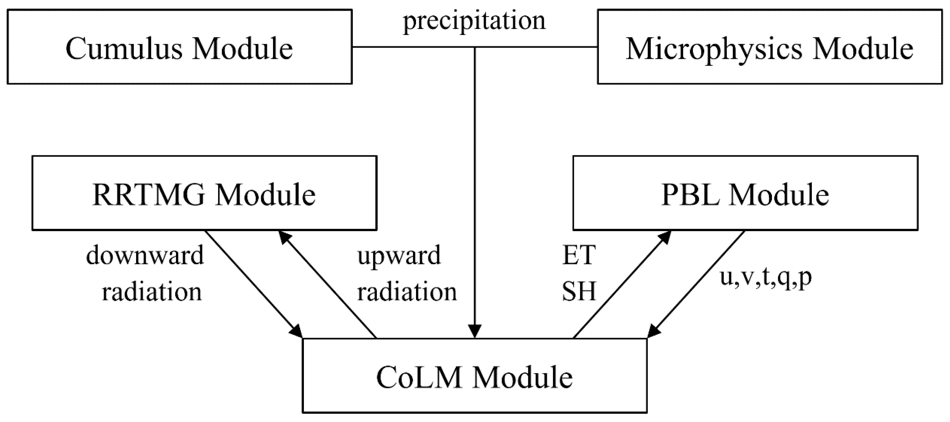
2.1. Models

2.1.1. GRAPES

Developed by the China Meteorological Administration [13], the Global/Regional Data Assimilation and Prediction System (GRAPES) has already been put into formal weather forecast operation in China [8]. The GRAPES model has a global version (GRAPES_GFS) and a mesoscale regional (GRAPES_Meso) version [14].

The GRAPES model used in this study is the global version, GRAPES_GFS-2-1-2-2 (hereinafter referred to as GRAPES). Currently, the highest horizontal resolution sup-ported by GRAPES is 0.25° (longitude) × 0.25° (latitude), and the number of vertical layers is 60. GRAPES adopts a semi-implicit-semi-Lagrangian dynamical framework integration scheme [15]. As a weather forecast model, GRAPES also has a complete framework of physical processes. Different physical processes are divided into different modules, including Cumulus module for simulating large-scale precipitation processes, the Microphysics Module for computing cloud microphysical processes, the planetary boundary layer (PBL) module, the radiative transfer module, and the land surface module, each of which has several options. Currently, the default scheme of the land surface module of GRAPES is CoLM2005. As shown in Figure 1, CoLM has been coupled with GRAPES by transmitting variables with other physical modules.

2.1.2. CoLM and Its Upgrade

CoLM was developed by Dai et al. [10] on the basis of combining BATS [16], IAP94 [17], and LSM Version 1.0 [18]. CoLM has a special single-layer double-large-leaf model for calculating vegetation photosynthesis, stomatal conductance, leaf temperature, and energy flux [9], which can accurately simulate and describe global land surface processes. CoLM has been widely used in land surface studies and Earth System Models such as the Chinese Academy of Sciences Earth System Model (CAS-ESM) [19], the Beijing Normal University Earth System Model (BNU-ESM) [20], the Climate-Weather Research and Forecasting Model (CWRF) [21], etc. The current version of CoLM coupled in the GRAPES_GFS is CoLM2005, and we refer to the original GRAPES model as GRAPES_ORI in this paper. The latest version of CoLM is CoLM2014. We couple CoLM2014 with GRAPES which is referred to as the GRAPES_NEW in this paper.

CoLM2005 and CoLM2014 share a same soil layer structure of which soil is divided into ten layers vertically [10]. However, in order to facilitate matching with other land surface schemes in the GRAPES_GFS and GRAPES_Meso regional model (in which Noah is used as the land surface scheme), the soil temperature and moisture calculated by CoLM are interpolated to the depths of 0–10 cm, 10–40 cm, 40–100 cm, and 100–200 cm as the GRAPES forecast output.

Based on CoLM2014, we make a series of supplements and improvements relative to CoLM2005, especially for the global soil texture data based on the Global Soil Dataset for use in Earth System Models (GSDE, Shangguan et al., 2014), the improvement of the parameterization scheme for surface and subsurface runoff, and a new version of lake model (CoLM_Lake). The supplements and improvements are listed below.

• Update of Global Soil Texture

The soil texture data used in CoLM for estimations of soil thermal and hydraulic parameters include the mass percentage of the three types of soil particles (i.e., clay%, silt%, and sand%). The Global Soil Dataset for use in Earth System Models (GSDE, [22]), which provides soil information including soil particle-size distribution, organic carbon, and nutrients with the global resolution of 1 km, has been widely used in land surface models (CoLM 2014, Noah, Noah-MP, BCC_AVIM 1.1), Earth System Models (CAS_ESM, BNU_ESM), and weather and climate models (WRF, CWRF, BCC_CSM) [23]. Therefore, we updated the soil texture data of GRAPES based on the soil texture data of the GSDE dataset.

In CoLM, the change in soil texture data directly affects the changes in soil hydraulic and thermal parameters, such as saturated soil volumetric water content ${\mathsf{\theta }}_{\mathrm{s}}$, saturated soil water potential ${\mathsf{\psi }}_{\mathrm{s}}$, and saturated hydraulic conductivity ${\mathrm{K}}_{\mathrm{s}}$; the calculation of soil hydraulic and thermal parameters adopts empirical formulas proposed by Cosby et al. [24]. These changes in soil hydraulic and thermal parameters then further affect the calculation of soil water and thermal profiles.

2.

Improvement of Parameterization Scheme for Surface and Subsurface Runoff

The surface and subsurface runoff parameterization scheme of CoLM2005 adopts the runoff model from BATS [16], while CoLM2014 adopts the SIMTOP model [25]. Although the above two schemes are improved based on the TOPMODEL [26], they have significant differences.

In a model grid box, the effective rainfall W_g is

$${\mathrm{W}}_{\mathrm{g}}{=\mathrm{P}}_{\mathrm{g}}{+\mathrm{M}}_{\mathrm{g}}$$

(1)

where P_g is the precipitation that reaches the soil surface after being intercepted by the vegetation canopy, and M_g is the melted snow water on the surface.

In CoLM2005, the groundwater level ${\mathrm{z}}_{\mathrm{w}}$ (Units: m) is described as

$${\mathrm{z}}_{\mathrm{w}}{=\mathrm{f}}_{\mathrm{z}}·\left({\mathrm{z}}_{\mathrm{bot}}-{{\displaystyle \sum }}_{\mathrm{j}}{\mathsf{\theta }}_{\mathrm{j}}\Delta {\mathrm{z}}_{\mathrm{j}}\right)$$

(2)

where ${\mathrm{f}}_{\mathrm{z}}$ = 1 ${\mathrm{m}}^{-1}$ is the depth scale parameter of the groundwater table, ${\mathrm{z}}_{\mathrm{bot}}$ is the depth of the bottom soil layer, $\Delta {\mathrm{z}}_{\mathrm{j}}$ is the thickness of soil layer j, and ${\mathsf{\theta }}_{\mathrm{j}}$ is the soil volumetric water content of soil layer j.

In CoLM2014, ${\mathrm{z}}_{\mathrm{w}}$ is diagnosed based on both effects of the groundwater recharge and the subsurface runoff caused by topographic distribution. The groundwater table rises as the groundwater is recharged by the outflow of soil water at the bottom layer, and declines with the groundwater routing to river as base flow.

In CoLM2005, the calculation of surface runoff does not explicitly consider the soil infiltration capacity, and the surface runoff ${\mathrm{R}}_{\mathrm{s},\mathrm{ori}}$ is calculated as

$${\mathrm{R}}_{\mathrm{s},\mathrm{ori}}{=\mathrm{f}}_{\mathrm{s},\mathrm{ori}}·{\mathrm{W}}_{\mathrm{g}}+\left(1-{\mathrm{f}}_{\mathrm{s},\mathrm{ori}}\right)·{\overline{{\mathrm{w}}_{\mathrm{s}}}}^4·{\mathrm{W}}_{\mathrm{g}}$$

(3)

where $\overline{{\mathrm{w}}_{\mathrm{s}}}$ is the soil layer thickness weighted soil wetness in the top three layers, while

$${\mathrm{f}}_{\mathrm{s},\mathrm{ori}}{=\mathrm{f}}_{\mathrm{wet}}·\exp \left(-{\mathrm{z}}_{\mathrm{w}}\right)$$

(4)

is the fraction of the saturated area in the grid box, and ${\mathrm{f}}_{\mathrm{wet}}$ = 0.3 is the proportion of the area with higher groundwater table in the grid, which is determined by the distribution of the topographic index.

The subsurface runoff can be described by Equation (5)

$${\mathrm{R}}_{\mathrm{b},\mathrm{ori}}{=\mathrm{K}}_{\mathrm{D}}·{\overline{{\mathrm{w}}_{\mathrm{b}}}}^{(2\mathrm{B}+3)}{+\mathrm{l}}_{\mathrm{b}}·\exp \left(-{\mathrm{z}}_{\mathrm{w}}\right)$$

(5)

where ${\mathrm{K}}_{\mathrm{D}}$ = 4 × ${10}^{-2}$ mm∙${\mathrm{s}}^{-1}$ is the saturated soil hydraulic conductivity of the bottom layer, $\overline{{\mathrm{w}}_{\mathrm{b}}}$ is the soil layer thickness and hydraulic conductivity weighted soil wetness in the bottom five layers, ${\mathrm{l}}_{\mathrm{b}}$ = ${10}^{-5}$ mm∙${\mathrm{s}}^{-1}$ is the saturated subsurface runoff coefficient estimated from soil and topographic characteristics, and B is the parameter in the soil retention relationship defined by Clapp and Hornberger [27].

In CoLM2014, all the effective rainfall in the saturated area in a grid box is converted into runoff as in CoLM2005, and the effective rainfall in the unsaturated area is partially converted into runoff based on the explicit consideration of soil infiltration capacity as follows:

$${\mathrm{R}}_{\mathrm{s},\mathrm{new}}{=\mathrm{f}}_{\mathrm{s},\mathrm{new}}·{\mathrm{W}}_{\mathrm{g}}+\left(1-{\mathrm{f}}_{\mathrm{s},\mathrm{new}}\right)·{(\mathrm{W}}_{\mathrm{g}}-{\mathrm{Q}}_{\max })$$

(6)

where Q_max is the soil maximum infiltration capacity, which is jointly determined by the saturated hydraulic conductivity ${\mathrm{K}}_{\mathrm{s},\mathrm{j}}$ and the volume fraction of ice particles in the soil pores ${\mathrm{V}}_{\mathrm{ice},\mathrm{j}}$ of the top three soil layers:

$${\mathrm{Q}}_{\max }=\min \left\{{\mathrm{K}}_{\mathrm{s},\mathrm{j}}·{10}^{-6·{\mathrm{V}}_{\mathrm{ice},\mathrm{j}}}\right\}\mathrm{j}=1,2,3$$

(7)

The fraction of the saturated area in the grid box (i.e., ${\mathrm{f}}_{\mathrm{s},\mathrm{new}}$) in Equation (6) are presented by

$${\mathrm{f}}_{\mathrm{s},\mathrm{new}}{=\mathrm{f}}_{\mathrm{wet}}·\exp \left(-0.5·\mathrm{fff}·{\mathrm{z}}_{\mathrm{w}}\right)$$

(8)

where $\mathrm{fff}$ is the decay factor for runoff.

As for the calculation of the subsurface runoff ${\mathrm{R}}_{\mathrm{b},\mathrm{new}}$, CoLM2014 comprehensively considers the subsurface runoff caused by topographic distribution:

$${\mathrm{R}}_{\mathrm{b},\mathrm{new}}{=\mathrm{f}}_{\mathrm{ice}}·{\mathrm{R}}_{\mathrm{drai},\max }·\exp \left(-{\mathrm{f}}_{\mathrm{drai}}·{\mathrm{z}}_{\mathrm{w}}\right)$$

(9)

where ${\mathrm{f}}_{\mathrm{ice}}$ represents the resistance of ice to subsurface runoff, ${\mathrm{f}}_{\mathrm{drai}}$ = 2.5 ${\mathrm{m}}^{-1}$ is the runoff attenuation factor, and ${\mathrm{R}}_{\mathrm{drai},\max }$ is the maximum subsurface runoff value.

3.

Update of CoLM Lake Model

The lake model of CoLM2005 adopts the lake scheme of the Bonan [28] LSM model. It divides lakes into deep lakes and shallow lakes with a fixed depth, and only divides lakes into six layers in one dimension, with some lake characteristics (e.g., extinction coefficient and roughness) set to be constant. The physical process of the CoLM2005 lake model only considers the molecular diffusion and eddy diffusion processes for energy transport, and does not consider the vertical mixing and eddy diffusion processes of shallow lakes. The lake temperature T is obtained by solving the following equation:

$$\frac{\partial \mathrm{T}}{\partial \mathrm{t}}=-\frac{\partial }{\partial \mathrm{z}}\left[\left({\mathrm{k}}_{\mathrm{m}}{+\mathrm{k}}_{\mathrm{e}}\right)\frac{\partial \mathrm{T}}{\partial \mathrm{z}}\right]+\frac{1}{{\mathrm{c}}_{\mathrm{w}}}\frac{\mathrm{d}\mathsf{\Phi }}{\mathrm{dz}}$$

(10)

where t is the time, z is the depth of the lake, ${\mathrm{c}}_{\mathrm{w}}$ is the heat capacity of water, ${\mathrm{k}}_{\mathrm{m}}{=\mathrm{k}}_{\mathrm{w}}·{\mathrm{c}}_{\mathrm{w}}{}^{-1}$ is the molecular diffusion coefficient (where ${\mathrm{k}}_{\mathrm{w}}$ is the thermal conductivity of water), ${\mathrm{k}}_{\mathrm{e}}$ is the eddy diffusion coefficient, and Φ is shortwave radiation absorbed by lakes.

Based on the eddy diffusion scheme of Hostetler and Bartlein [29], the stratification scheme of Henderson-Sellers [30], and the lake–atmosphere feedback scheme of Bonan [28] and Hostetler et al. [31,32], a new generation lake model CoLM_Lake, which is the lake model of CoLM2014, has been developed by Dai et al. [33]. CoLM_Lake divides the lake into 10 layers, with at most 5 snow layers and 10 mud layers above and below the lake system, respectively.

The updates of CoLM_Lake relative to the original model can be summarized as follows: (1) the interaction between precipitation and lake surface is included, with a detailed description of the precipitation effect on snow freeze–thaw processes; (2) the settings of lake parameters are changed from constant to dynamic diagnosis based on lake features and lake states, for example, the lake surface roughness length is determined by both the air conditions above lakes and lake surface properties, and the extinction coefficient η for lake absorption of solar radiation changes with the lake depth; (3) the lake temperature for the first layer and at the surface is adjusted based on the thermal stability; (4) the lake stratification is setting based on the lake depth instead of fixed stratification; (5) the freezing–thawing process and the vertical mixing process of lake water depending on the density and lake ice fractions are specifically described, in which the vertical mixing process is driven by three factors: the liquid water molecular diffusion, the eddy diffusion driven by lake surface wind, and other processes which can enhance mixing but cannot expressed explicitly in the model; (6) the intensity of vertical mixing of the deep lake is enhanced according to the lake depth.

Dai et al. [33] evaluated CoLM_Lake using observation data from ten lakes, and found that CoLM_Lake can accurately simulate the surface temperature and vertical thermal structure of lakes, and reasonably describe the main characteristics of lakes such as seasonal freeze–thaw cycles.

2.2. Experimental Design

GRAPES_ORI and GRAPES_NEW were run from 20 July 2016 to 1 September 2016 with the initial field coming from NCEP FNL reanalysis data [34], which are widely used in the assessment of GRAPES_GFS [35]. The forecast started at 12:00 (universal time) every day, with a forecast duration of 8 days. The model parameter settings for GRAPES operation are shown in

Table 1. Model parameters used in GRAPES forecast run.

Model Parameters	GRAPES_ORI	GRAPES_NEW
Horizontal Resolution	0.25° × 0.25°	0.25° × 0.25°
Vertical Layers	60	60
Integration Time Step	300 s	300 s
Microphysics Scheme	WSM6 [36]	WSM6
Cumulus Scheme	Simplified Arakawa-Schubert Scheme [37,38]	Simplified Arakawa-Schubert Scheme
Radiation Scheme	RRTMG [39,40]	RRTMG
PBL Scheme	MRF PBL Scheme [41]	MRF PBL Scheme
Land Surface Scheme	CoLM2005	CoLM2014

below. All parameters adopted for the experiments were set the same as the default setups for the current forecast operation of GRAPES_GFS, except for the differences between the land surface schemes, which have been described in the previous section.

The global forecast outputs of GRAPES_ORI and GRAPES_NEW are on a resolution of 0.25° (latitude) × 0.25° (longitude). Key atmospheric variables (i.e., geopotential height at 500 hPa and 850 hPa, wind speed at 10 m, air temperature at 2 m, and precipitation) and land variables (i.e., surface soil moisture, surface soil temperature, evapotranspiration, and sensible heat flux) from the GRAPES_ORI and GRAPES_NEW forecast output are evaluated in this paper.

2.3. Validation Datasets

Validation data used for geopotential height at 500 hPa and 850 hPa, wind speed at 10 m, and air temperature at 2 m data were obtained from the ERA5 datasets [42] provided by the European Centre for Medium-range Weather Forecasts (ECMWF) at hourly resolution on a global 0.25° × 0.25° spatial grid, and these data are from (https://cds.climate.copernicus.eu/cdsapp#!/dataset/reanalysis-era5-pressure-levels?tab=form) (accessed on 20 May 2021) and (https://cds.climate.copernicus.eu/cdsapp#!/dataset/reanalysis-era5-single-levels?tab=form) (accessed on 21 May 2021).

The precipitation validation data are from the 3rd level of Integrated Multi-satellite Retrievals for Global Precipitation Measurement (GPM) Final Precipitation dataset at half-hourly resolution (GPM_3IMERGHH). Developed by the National Aeronautics and Space Administration (NASA), the GPM dataset uses both satellite microwave and microwave-calibrated infrared (IR) estimates, together with gauge calibration to estimate the global precipitation [43], and is widely used for global precipitation research [44]. The GPM precipitation data are on a global 0.1° × 0.1° grid, which were acquired from (https://gpm1.gesdisc.eosdis.nasa.gov/data/GPM_L3/GPM_3IMERGHH.06/2016/) (accessed on 16 September 2021).

The Global Land Data Assimilation System (GLDAS), also developed by NASA [45], fusing remote sensing and ground-based observations, produces land surface variables, such as soil moisture and evapotranspiration [46]. The GLDAS data are widely used in land surface research [47,48,49,50] with an acceptable evaluation by researchers [51,52,53,54]. The GLDAS data we used for validation are 3-hourly surface soil moisture, surface soil temperature, evapotranspiration, and sensible heat flux data from GLDAS_NOAH025_3H (https://hydro1.gesdisc.eosdis.nasa.gov/data/GLDAS/GLDAS_NOAH025_3H.2.1/2016/) (accessed on 24 September 2021), which covered 60° S–90° N latitudes on a 0.25° × 0.25° grid.

All of the validation data cover from 27 July 2016 to 1 September 2016.

2.4. Data Processing and Evaluation Metrics

All validation data are interpolated into 0.25° × 0.25° by the local area-averaging method. Due to the missing values of GPM precipitation data in the near-polar areas [55], we used the 55° S–55° N latitudes as the study areas in precipitation evaluation, while other variables cover from 60° S to 90° N. The spatial distributions of GRAPES forecast outputs are evaluated against daily fields from the validation data.

In this paper, the anomaly correlation coefficient (ACC) [56] is used to characterize the similarity of the anomaly distributions of the two fields. ACC is commonly used in the evaluation of model prediction capacity [57,58]. The closer the ACC value is to 1, the higher the similarity of the two-variable field anomaly distribution is. In forecast verification, when the ACC is greater than 0.6, the forecast is usually considered to be successful, or the variable is predictable by the model [58,59]. We also introduce the root mean square error (RMSE) [60] in this paper to evaluate the average closeness of the forecast results to the validation datasets. Smaller values of RMSE mean smaller deviation between the forecast field and the validation field. The calculation of ACC and RMSE can be expressed by:

$$\mathrm{ACC}=\frac{{{\displaystyle \sum }}_{\mathrm{i}}\left({\mathrm{y}}_{\mathrm{ip}}-{{\displaystyle \overline{\mathrm{y}}}}_{\mathrm{ip}}\right)\left({\mathrm{y}}_{\mathrm{iv}}-{{\displaystyle \overline{\mathrm{y}}}}_{\mathrm{iv}}\right)}{\mathrm{N}\sqrt{\frac{1}{\mathrm{N}}{{\displaystyle \sum }}_{\mathrm{i}}{\left({\mathrm{y}}_{\mathrm{ip}}-{{\displaystyle \overline{\mathrm{y}}}}_{\mathrm{ip}}\right)}^2}\sqrt{\frac{1}{\mathrm{N}}{{\displaystyle \sum }}_{\mathrm{i}}{\left({\mathrm{y}}_{\mathrm{iv}}-{{\displaystyle \overline{\mathrm{y}}}}_{\mathrm{iv}}\right)}^2}}$$

(11)

$$\mathrm{RMSE}=\sqrt{\frac{1}{\mathrm{N}}{\displaystyle \sum }_{\mathrm{i}}{\left({\mathrm{y}}_{\mathrm{ip}}-{\mathrm{y}}_{\mathrm{iv}}\right)}^2}$$

(12)

where ${\mathrm{y}}_{\mathrm{ip}}$ is the predicting result at grid point i, ${\mathrm{y}}_{\mathrm{iv}}$ is the corresponding validation field, and N stands for the total number of prediction times corresponding to the grid point.

The study areas contain global (60° S–90° N, 180° W–180° E), Northern Hemisphere (0°–90° N, 180° W–180° E), Southern Hemisphere (60° S–0°, 180° W–180° E), and East Asia (15°–55° N, 70°–140° E) when calculating regional averaged values, except for precipitation whose study areas are set to Global (55° S–55° N, 180° W–180° E), Northern Hemisphere (0°–55° N, 180° W–180° E), Southern Hemisphere (55° S–0°, 180° W–180° E), and East Asia (15°–55° N, 70°–140° E), respectively.

In particular, the verification of precipitation forecasting includes some special methods. In the contingency table for precipitation (

Table 2. A 2 × 2 contingency table for precipitation.

Precipitation Events		Events Happened
		Yes	No
Events Forecasted	Yes	${\mathrm{N}}_{\mathrm{h}}$	${\mathrm{N}}_{\mathrm{f}}$
	No	${\mathrm{N}}_{\mathrm{m}}$	${\mathrm{N}}_{\mathrm{cn}}$

), ${\mathrm{N}}_{\mathrm{h}}$ is the number of accurate forecasts of events that happened (hits), ${\mathrm{N}}_{\mathrm{f}}$ is the number of forecasts of events that did not happen (false alarms), ${\mathrm{N}}_{\mathrm{m}}$ is the number of events that happened but were not forecasted (missing alarms), and ${\mathrm{N}}_{\mathrm{cn}}$ is the number of correct forecasts of events that did not happen (correct negatives).

Threat score (TS) [61], bias score (BIAS) [62], probability of false alarms (POFA) [63], and probability of missing alarms (POMA) are commonly used for precipitation forecast verification by the National Meteorological Center of China [64], and could be described as follows:

$$\mathrm{TS}=\frac{{\mathrm{N}}_{\mathrm{h}}}{{\mathrm{N}}_{\mathrm{h}}{+\mathrm{N}}_{\mathrm{f}}{+\mathrm{N}}_{\mathrm{m}}}$$

(13)

$$\mathrm{BIAS}=\frac{{\mathrm{N}}_{\mathrm{h}}{+\mathrm{N}}_{\mathrm{f}}}{{\mathrm{N}}_{\mathrm{h}}{+\mathrm{N}}_{\mathrm{m}}}$$

(14)

$$\mathrm{POFA}=\frac{{\mathrm{N}}_{\mathrm{f}}}{{\mathrm{N}}_{\mathrm{h}}{+\mathrm{N}}_{\mathrm{f}}}$$

(15)

$$\mathrm{POMA}=\frac{{\mathrm{N}}_{\mathrm{m}}}{{\mathrm{N}}_{\mathrm{h}}{+\mathrm{N}}_{\mathrm{m}}}$$

(16)

A closer value of TS to 1 indicates the higher proportion of accurate forecasts. The closer the BIAS is to 1, the more stable the forecast is presented. POFA represents the model’s over-prediction of precipitation, and POMA is often used with POFA, which reflects the model’s underestimation of precipitation.

The TS, BIAS, POFA, and POMA of precipitation were calculated towards different regions at different rain levels (i.e., light rain ranges 0.1–9.9 mm, moderate rain ranges 10.0–24.9 mm, heavy rain ranges 25.0–49.9 mm, and extreme rainfall ranges over 50.0 mm within 24 h).

3. Results

3.1. Atmospheric Variables

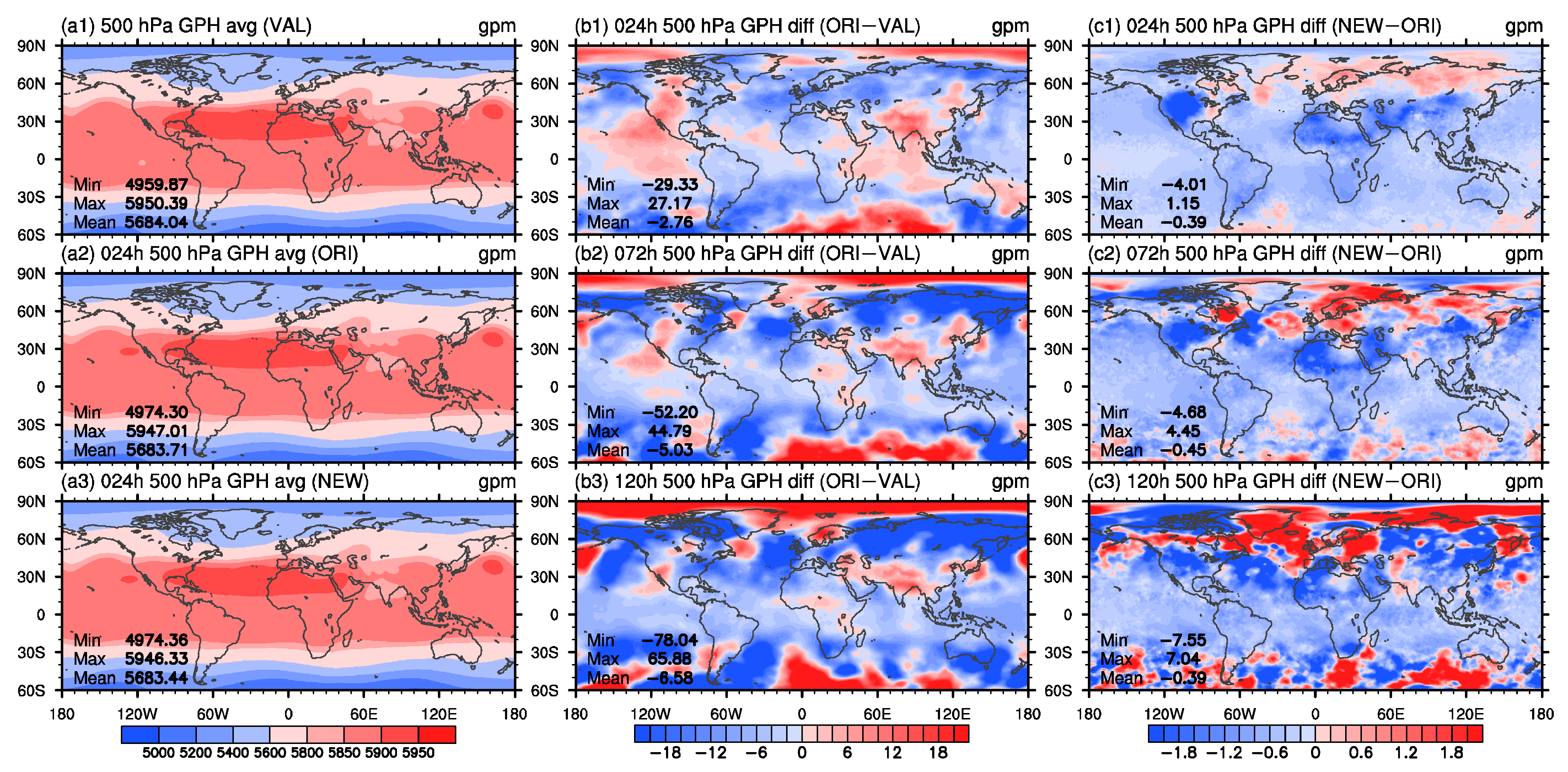
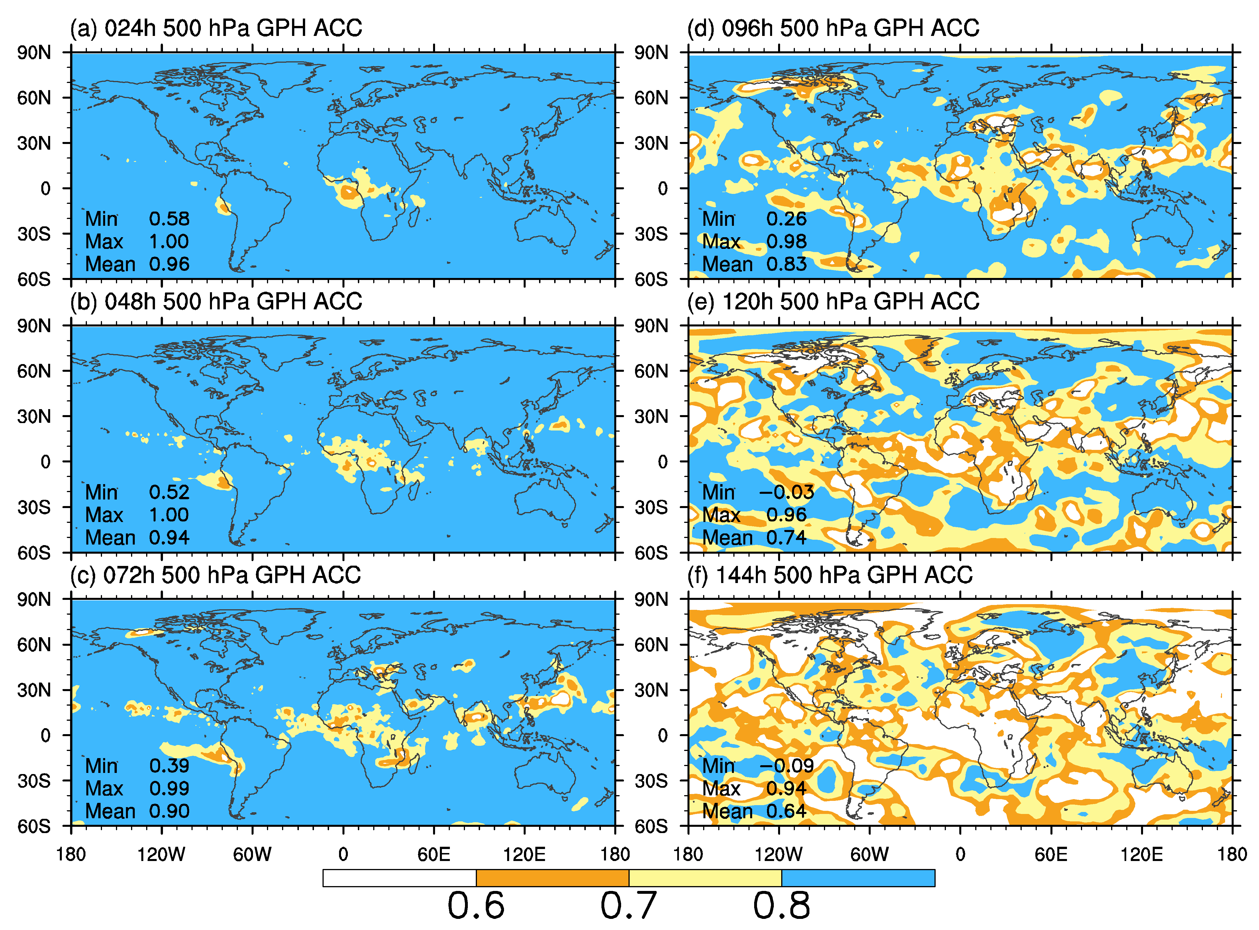
3.1.1. Geopotential Height

The spatial distribution of the geopotential height at 500 hPa (H500) indicates the large-scale circulation pattern, and also influences the regional weather and climate [65,66,67]. H500 represents the vital weather systems such as the position of ridge and trough [68], the pattern of summer monsoon precipitation [69], and the strength and position of western Pacific subtropical high (WPSH) [70]. Therefore, the accuracy and stability of H500 is a good criterion for evaluating the performance of weather and climate models.

The predicted results of H500 are shown in Figure 2. Compared with the ERA5 reanalysis dataset, the 24 h forecasting results from GRAPES_ORI and GRAPES_NEW models can both reproduce the spatial patterns of H500 field (Figure 2(a1–a3)). The high values spread from northeast America to the Middle East through the western Pacific along the 30° N latitudinal band, while the low values mainly locate over polar zones. The middle column of Figure 2 shows the differences in H500 between GRAPES_ORI results and ERA5 for different forecast lengths. In 24 h forecasting results, the GRAPES_ORI shows a relative overestimation, with about 5 gpm over the western part of North America, the eastern part of the Pacific Ocean, southwestern China, and India, while over the eastern part of North America, Africa, and northern Eurasia, H500 is slightly underestimated, with about 6 gpm (Figure 2(b1)). The 72 h and 120 h forecasting results show similar spatial patterns with a larger magnitude of differences. The right column of Figure 2 shows the differences between GRAPES_ORI and GRAPES_NEW forecasts. The GRAPES_NEW results show a higher value over the northern Eurasian continent, which correct the low biases in GRAPES_ORI. Similarly, over western North America, North Africa, and central Asia, the GRAPES_NEW also corrects the results from GRAPES_ORI by reducing the overestimation in GRAPES_ORI. With the growing of forecasting hours, the prediction errors of GRAPES_ORI increase, especially over the mid–high latitude. The corresponding errors in GRAPES_NEW also increase gradually. Overall, results of H500 from GRAPES_NEW correct the prediction error in GRAPES_ORI over most regions, revealing a better performance of GRAPES_NEW.

The spatial distribution of ACC for H500 between GRAPES_NEW and ERA5 is given by Figure 3. The higher ACC values, the more similar of the anomalies in GRAPES_NEW to that in ERA5. The global-averaged ACC is greater than 0.6 for the prediction within 6 days. When the prediction time comes to 5 or 6 days, the area with low ACC values expands.

In one word, the GRAPES_NEW has good performance on H500 predictions, even though the errors grow with prediction hours. Similar conclusions can also be obtained from the analyses for geopotential height at 850 hPa (H850) predictions (not shown).

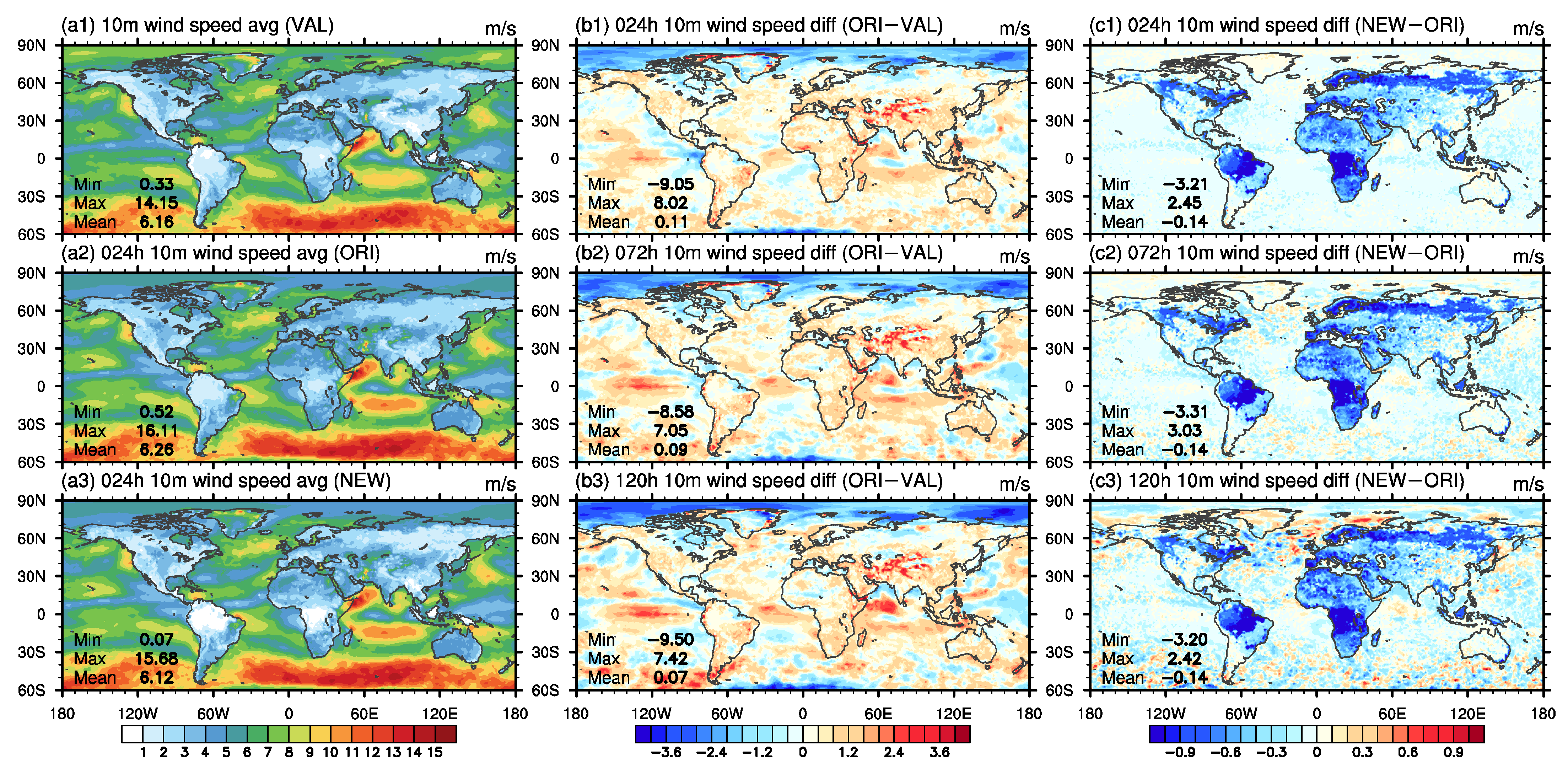
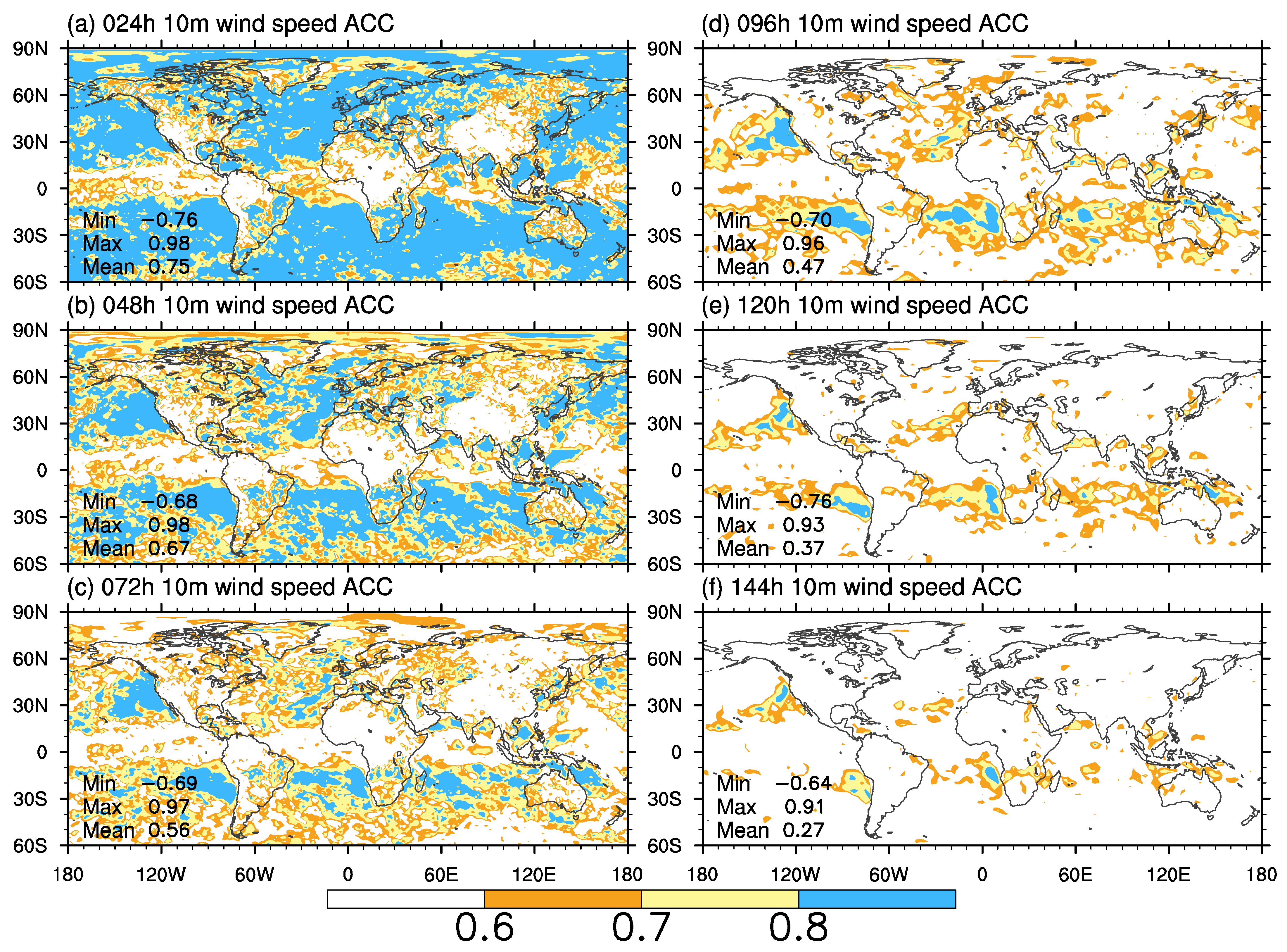
3.1.2. Wind Speed at 10 m

The surface wind influences the water/heat transfer and land–atmosphere coupling [71], which is required to evaluate its performance in the model simulation. As seen from Figure 4(a1–a3), the prediction result from GRAPES_ORI and GRAPES_NEW can reproduce the general distribution of spatial patterns, including the overall differences in wind speed between ocean and land surface. Compared with ERA5, GRAPES_ORI has an overestimation (+1.2 m∙${\mathrm{s}}^{-1}$) on the global mean wind speed, especially over the Arabian Sea, tropical Indian Ocean, central Pacific Ocean, and Tibetan Plateau region (Figure 4(b1–b3)). The GRAPES_NEW has little improvement over oceans compared to GRAPES_ORI, but over the land, GRAPES_NEW shows significantly decreased wind speed, especially over central Africa, the Amazon, and the mid–high latitudes over the Northern Hemisphere (Figure 4(c1–c3)). Moreover, unlike the H500 and H850 field, the prediction error of 10 m wind speed shows insignificant changes as the forecasting hour grows in both GRAPES_ORI (Figure 4(b1–b3)) and GRAPES_NEW (Figure 4(c1–c3)).

Figure 5 is given by the spatial distribution of ACC for 10 m wind speed in different forecasting hours. The subtropical region shows a large ACC value greater than 0.6 while the tropical region shows a smaller ACC value, which indicates that the 10 m wind speed retains a better performance in the mid–high latitudes but a poor performance in the tropical regions.

To further evaluate the surface wind speed performance over different regions, we calculated the area-averaged ACC, as shown in

Table 3. ACC of wind speed at 10 m between GRAPES forecast and ERA5 over different regions.

Forecast Length (Units: h)	Global		Southern Hemisphere		Northern Hemisphere		East Asia
	ORI	NEW	ORI	NEW	ORI	NEW	ORI	NEW
24	0.7521	0.7532	0.7295	0.7312	0.7861	0.7863	0.5978	0.5997
48	0.6662	0.6672	0.6397	0.6411	0.7061	0.7064	0.5307	0.5333
72	0.5636	0.5644	0.5291	0.5303	0.6154	0.6155	0.4467	0.4478
96	0.4631	0.4651	0.4245	0.4273	0.5210	0.5218	0.3596	0.3602
120	0.3664	0.3660	0.3284	0.3279	0.4233	0.4230	0.2780	0.2793
144	0.2748	0.2740	0.2361	0.2348	0.3328	0.3329	0.2191	0.2143
168	0.2078	0.2052	0.1820	0.1791	0.2467	0.2444	0.1766	0.1696
192	0.1474	0.1485	0.1295	0.1303	0.1743	0.1758	0.1328	0.1314

. It is clear that ACC decreases rapidly as the forecasting hours grow. The ACC is mostly greater than 0.6 when the forecasting hours are less than 72 h, which indicates that the surface wind speed is predictable on continental scales within 3 days. The ACC of the Northern Hemisphere is worse than the Southern Hemisphere, which may relate to the rapid change in surface wind due to strong convective activities in the boreal summer. Additionally, the ACC derived from GRAPES_NEW is larger than that from GRAPES_ORI in most regions and forecast lengths, which shows an improvement of surface wind speed prediction in GRAPES_NEW.

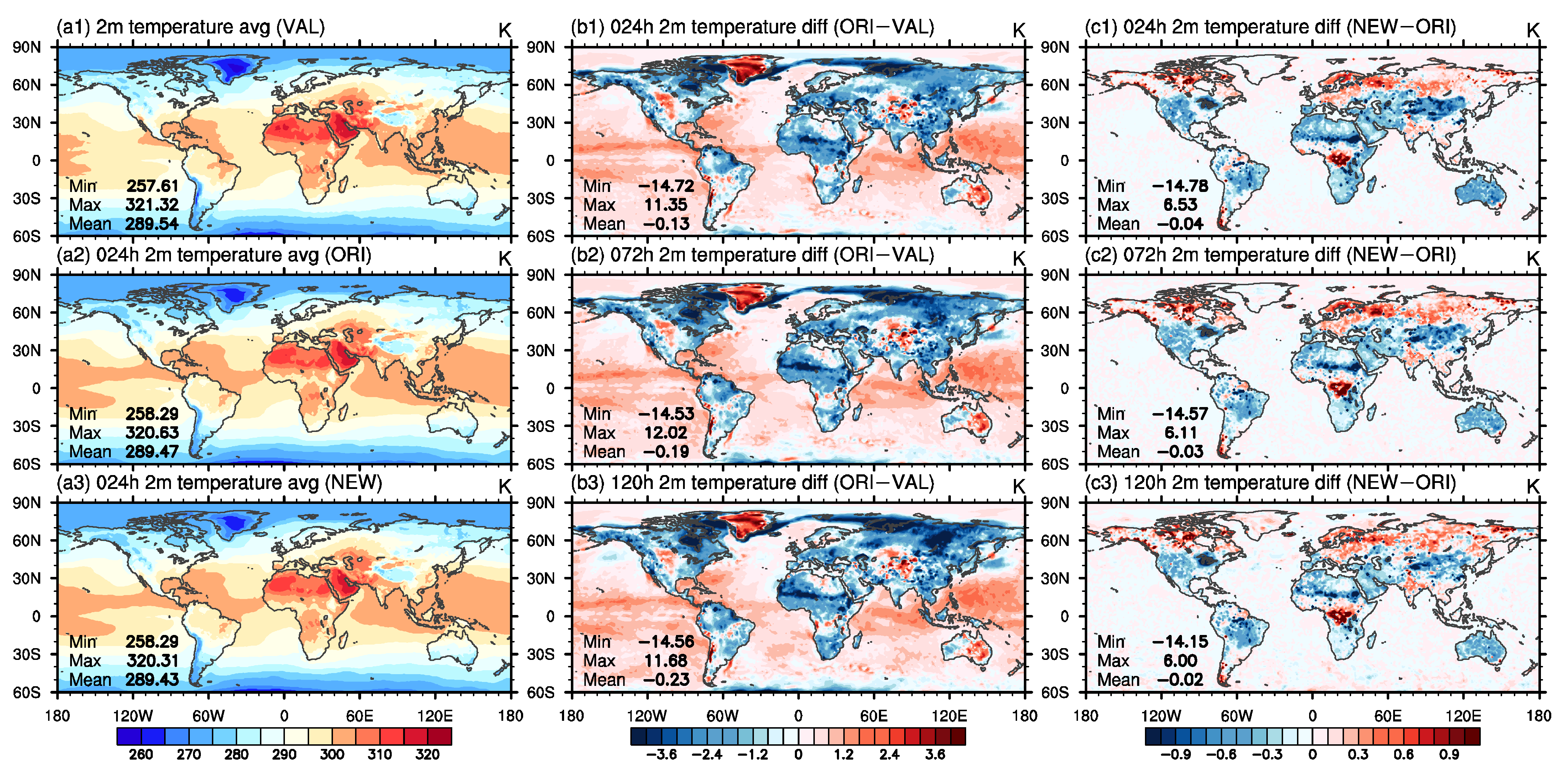
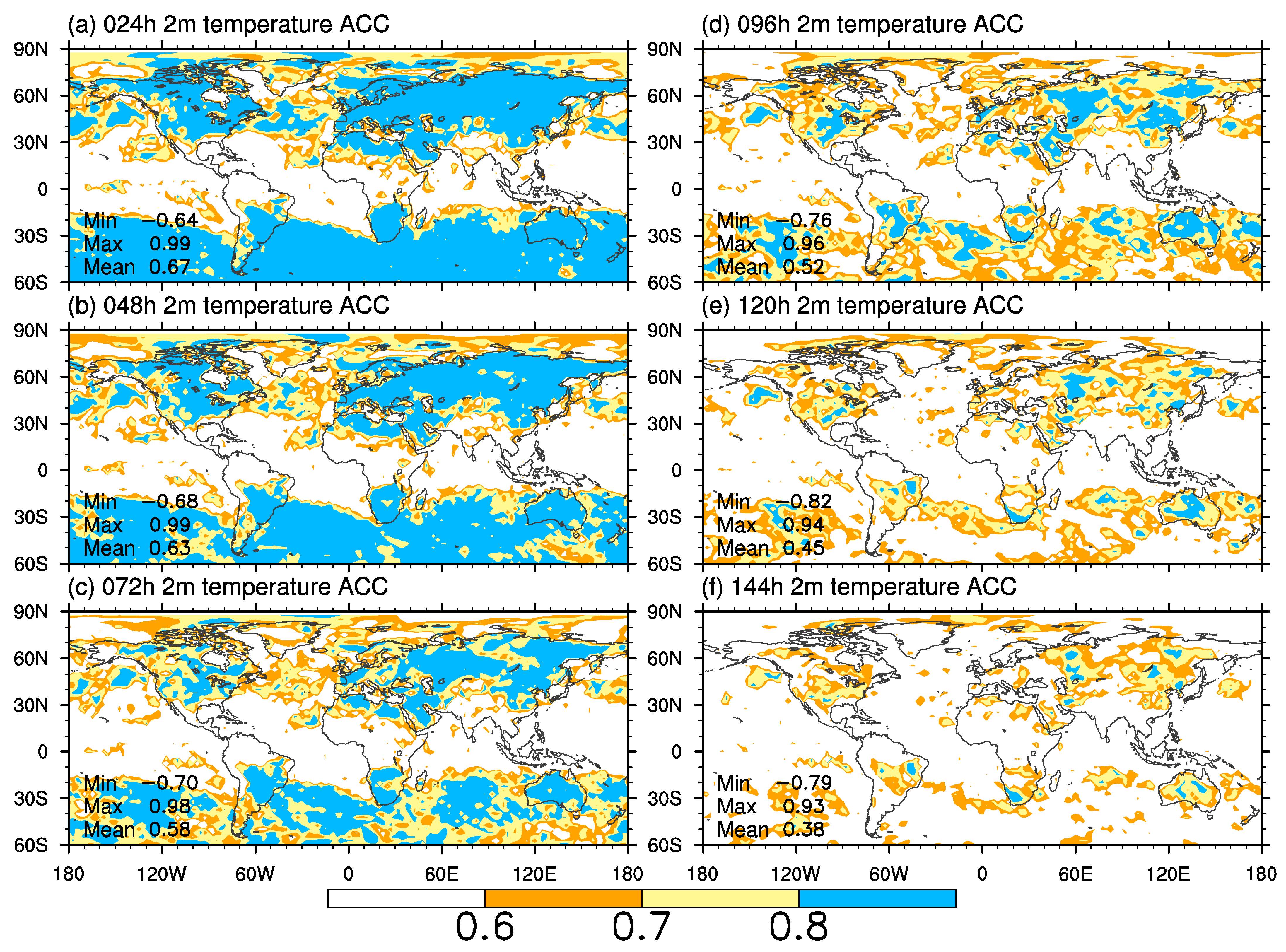
3.1.3. Air Temperature at 2 m

The surface air temperature is crucial for ecosystem and human activities [72]. The results show that both GRAPES_ORI and GRAPES_NEW can reproduce the spatial distribution of surface air temperature (Figure 6(a1–a3)). Compared to ERA5, GRAPES_ORI shows significant underestimation over land and overestimation over tropical oceans (Figure 6(b1–b3)). The cold bias exists over the Northern Hemisphere with about 2 K. The GRAPES_NEW shows improvements over land, especially over the mid–high latitudes of the Northern Hemisphere, the Tibetan Plateau, and Australia, while the sea surface temperature has little change compared to GRAPES_ORI (Figure 6(c1–c3)). With the increase in forecasting hours, the prediction skill varies insignificantly in both GRAPES_ORI (Figure 6(b1–b3)) and GRAPES_NEW (Figure 6(c1–c3)).

The spatial distribution of ACC in 2 m temperature derived from GRAPES_NEW shows high skills over the extratropical region and low skills over the tropical regions, which is consistent with the relatively high prediction errors in tropical oceans. The global mean ACC values are close to or larger than 0.6 for the forecasts within 72 h, which indicates that GRAPES_NEW shows great prediction skill on 2 m air temperature within 3 days (Figure 7(a–c)). As the forecasting hours increase, the ACC remains 0.6 over part of regions such as North America, the Eurasian continent, and Australia, where the effective forecast length can reach 6 days.

In addition, we further calculate the area-averaged ACC over global, Northern Hemisphere, Southern Hemisphere, and eastern Asia, respectively. As shown in

Table 4. ACC of 2 m air temperature between GRAPES forecast and ERA5 over different regions.

Forecast Length (Units: h)	Global		Southern Hemisphere		Northern Hemisphere		East Asia
	ORI	NEW	ORI	NEW	ORI	NEW	ORI	NEW
24	0.6666	0.6665	0.6259	0.6260	0.7275	0.7274	0.6719	0.6726
48	0.6293	0.6293	0.5868	0.5867	0.6930	0.6931	0.6263	0.6287
72	0.5802	0.5803	0.5391	0.5394	0.6417	0.6416	0.5680	0.5718
96	0.5176	0.5182	0.4790	0.4799	0.5756	0.5755	0.5041	0.5099
120	0.4513	0.4518	0.4191	0.4195	0.4996	0.5002	0.4533	0.4525
144	0.3832	0.3837	0.3640	0.3638	0.4119	0.4135	0.4151	0.4141
168	0.3236	0.3224	0.3192	0.3181	0.3303	0.3288	0.3795	0.3769
192	0.2660	0.2636	0.2714	0.2680	0.2578	0.2569	0.3422	0.3430

, the ACC of 2 m air temperature decreases rapidly as the forecasting hours increase, and the predictable duration is about 3 days on a global scale. The ACC over eastern Asia is generally higher than other regions, with the values ranging from 0.6726 to 0.3422, which denotes a more stable prediction result for eastern Asia. The ACC values derived from GRAPES_NEW show improvements of forecasts within 5 days compared to GRAPES_ORI, and the similar results can also be obtained from the analysis for RMSE (not shown).

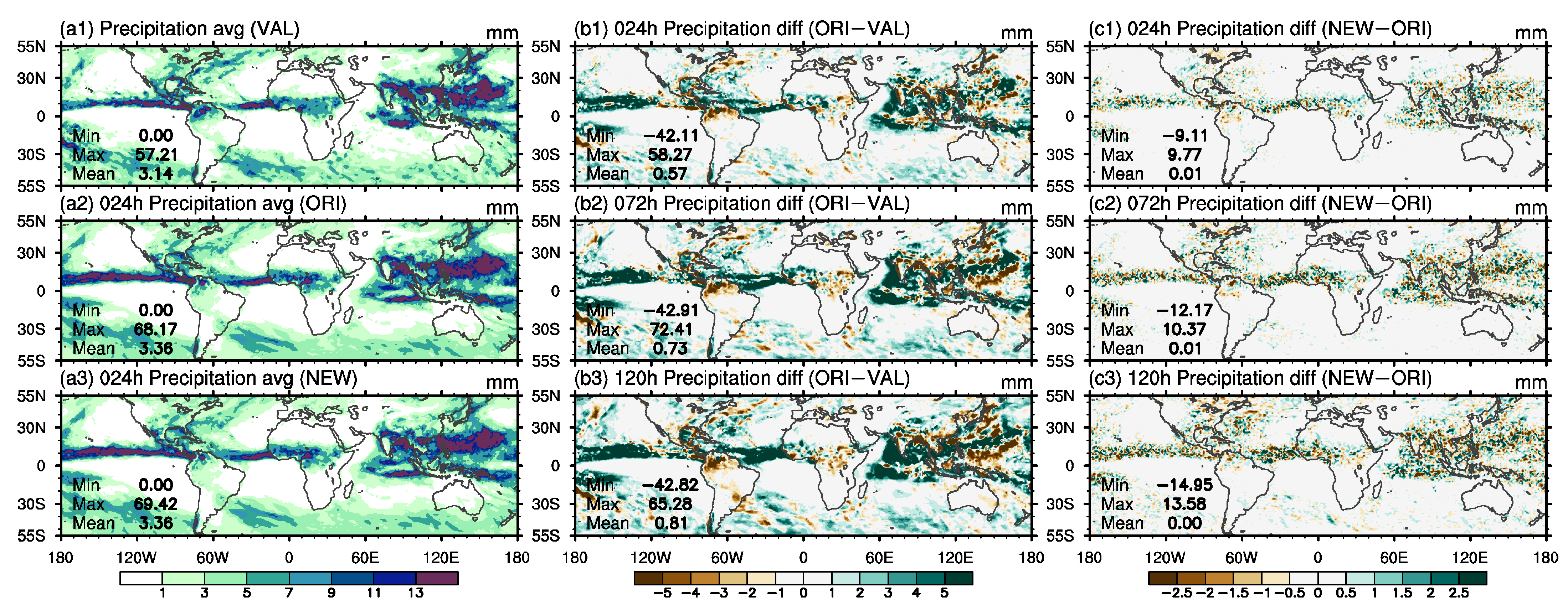
3.1.4. Precipitation

The precipitation forecasting performance of numerical weather prediction models is an important factor affecting the quantitative forecast quality of precipitation by forecasters [54]. The precipitation prediction of GRAPES has been evaluated by both case studies [73] and regional predictions [74], but the influences of land processes on precipitation predictions are few to be considered. Here, we quantify the prediction skill of precipitation by analyzing the climatology mean and adopting a series of indexes applied by the National Meteorological Center [64] such as threat score (TS), bias score (BIAS), probability of false alarm (POFA), and probability of missing alarm (POMA) to evaluate the forecasting results.

GRAPES can reproduce the global precipitation distribution with three main rain belts lying over the extratropical region of the Northern Hemisphere, the tropical region, and the mid–high latitude of the Southern Hemisphere (Figure 8(a1–a3)). GRAPES_ORI shows obvious overestimation in the tropical oceans, and the prediction error grows with longer forecasting hours (Figure 8(b1–b3)). Compared to GRAPES_ORI, GRAPES_NEW shows a relatively small improvement in tropical precipitation (Figure 8(c1–c3)).

Table 5. TS of precipitation at different rainfall levels over East Asia.

Rainfall Levels	Light Rain		Moderate Rain		Heavy Rain		Extreme Rainfall
Forecast Length (Units: h)	ORI	NEW	ORI	NEW	ORI	NEW	ORI	NEW
24	0.4582	0.4567	0.1268	0.1277	0.0975	0.0976	0.1375	0.1383
48	0.4411	0.4404	0.1148	0.1148	0.0798	0.0809	0.1250	0.1271
72	0.4221	0.4218	0.1025	0.1019	0.0674	0.0672	0.1079	0.1042
96	0.4062	0.4060	0.0924	0.0915	0.0553	0.0545	0.0805	0.0814
120	0.3900	0.3899	0.0842	0.0842	0.0488	0.0498	0.0630	0.0644
144	0.3846	0.3808	0.0826	0.0793	0.0445	0.0449	0.0523	0.0516
168	0.3735	0.3717	0.0751	0.0753	0.0369	0.0368	0.0354	0.0357
192	0.3732	0.3739	0.0729	0.0718	0.0332	0.0341	0.0276	0.0284

gives the TS of precipitation at different rainfall levels over eastern Asia. The prediction skill of GRAPES_NEW for rainfall level above heavy rain improved slightly within 48 forecasting hours, while for rainfall level at light rain and moderate rain, the prediction skill of GRAPES_NEW shows a comparable skill level with GRAPES_ORI. The bias score (BIAS) is given by

Table 6. BIAS of precipitation at different rainfall levels over East Asia.

Rainfall Levels	Light Rain		Moderate Rain		Heavy Rain		Extreme Rainfall
Forecast Length (Units: h)	ORI	NEW	ORI	NEW	ORI	NEW	ORI	NEW
24	1.0294	1.0270	1.2985	1.3081	1.0962	1.1100	0.7021	0.6949
48	1.0207	1.0244	1.3630	1.3811	1.1737	1.1681	0.8463	0.8364
72	1.0192	1.0232	1.3172	1.3317	1.1499	1.1447	0.8989	0.8787
96	1.0102	1.0143	1.2992	1.3112	1.1296	1.0992	0.8479	0.8346
120	1.0142	1.0145	1.3127	1.3178	1.1175	1.0926	0.8086	0.7947
144	1.0230	1.0178	1.3283	1.3284	1.0783	1.0764	0.8266	0.8070
168	1.0263	1.0193	1.3530	1.3591	1.0864	1.0743	0.7808	0.7427
192	1.0298	1.0238	1.3648	1.3532	1.0437	1.0146	0.6834	0.6194

, which also suggests that the prediction bias from GRAPES_NEW decreases for rainfall levels above heavy rain compared to GRAPES_ORI, which is consistent with the results from the TS table.

In addition, the POFA (

Table 7. POFA of precipitation at different rainfall levels over East Asia.

Rainfall Levels	Light Rain		Moderate Rain		Heavy Rain		Extreme Rainfall
Forecast Length (Units: h)	ORI	NEW	ORI	NEW	ORI	NEW	ORI	NEW
24	0.3787	0.3794	0.7998	0.7993	0.8283	0.8291	0.7077	0.7041
48	0.3929	0.3948	0.8204	0.8213	0.8609	0.8592	0.7475	0.7416
72	0.4107	0.4123	0.8355	0.8374	0.8803	0.8803	0.7904	0.7944
96	0.4243	0.4259	0.8489	0.8506	0.8996	0.8998	0.8362	0.8324
120	0.4411	0.4417	0.8617	0.8617	0.9084	0.9059	0.8565	0.8543
144	0.4490	0.4517	0.8642	0.8693	0.9156	0.9143	0.8831	0.8862
168	0.4613	0.4614	0.8766	0.8766	0.9286	0.9296	0.9161	0.9138
192	0.4635	0.4616	0.8799	0.8812	0.9354	0.9331	0.9317	0.9246

) and POMA (

Table 8. POMA of precipitation at different rainfall levels over East Asia.

Rainfall Levels	Light Rain		Moderate Rain		Heavy Rain		Extreme Rainfall
Forecast Length (Units: h)	ORI	NEW	ORI	NEW	ORI	NEW	ORI	NEW
24	0.3624	0.3645	0.7428	0.7401	0.8135	0.8121	0.7992	0.7982
48	0.3815	0.3811	0.7583	0.7563	0.8395	0.8376	0.8018	0.8002
72	0.4009	0.4000	0.7853	0.7853	0.8629	0.8637	0.8191	0.8262
96	0.4196	0.4187	0.8071	0.8081	0.8878	0.8912	0.8626	0.8614
120	0.4349	0.4351	0.8222	0.8216	0.9021	0.9010	0.8952	0.8934
144	0.4380	0.4435	0.8239	0.8299	0.9113	0.9109	0.9098	0.9114
168	0.4491	0.4529	0.8367	0.8358	0.9263	0.9256	0.9395	0.9408
192	0.4485	0.4496	0.8405	0.8436	0.9333	0.9321	0.9534	0.9548

), which represent the false alarm rate and missing ratio of model precipitation prediction with respect to the real precipitation events, also denote that during the whole forecasting length, GRAPES_NEW has a better performance on predictions of rainfall level above heavy rain, and a comparable performance on predictions of rainfall level below heavy rain compared to GRAPES_ORI.

Overall, the GRAPES_NEW shows a more precise and stable prediction on rainfall level above heavy rain over East Asia. We also evaluated the precipitation prediction skill over other regions (not shown), and found that GRAPES_NEW shows a better performance over the Southern Hemisphere than the Northern Hemisphere on the prediction skill of rainfall level below heavy rain, while for the rainfall level above heavy rain, GRAPES_NEW shows a better prediction skill over the Northern Hemisphere than that over the Southern Hemisphere.

Therefore, the GRAPES model shows a considerable ability to reproduce the precipitation distribution, even though the prediction skill decreases with the increase in rainfall level and forecasting hours. Compared with GRAPES_ORI, GRAPES_NEW shows improvements on rainfall levels above heavy rain in both accuracy and stability.

3.2. Land Variables

The surface soil layer is the interface of land and atmosphere for exchanging water and energy [75]. The surface soil moisture and soil temperature have a significant impact on precipitation [76] and other near-surface meteorology variables [77,78]. Evapotranspiration is also a key factor that links the water, energy, and carbon cycles [79]. It determines the water vapor exchange between land and atmosphere, and directly influences the precipitation [80,81]. Sensible heat flux represents the heat transfer between land and atmosphere. Therefore, it is necessary to evaluate the prediction skill of GRAPES on surface soil moisture, surface soil temperature, evapotranspiration, and sensible heat flux.

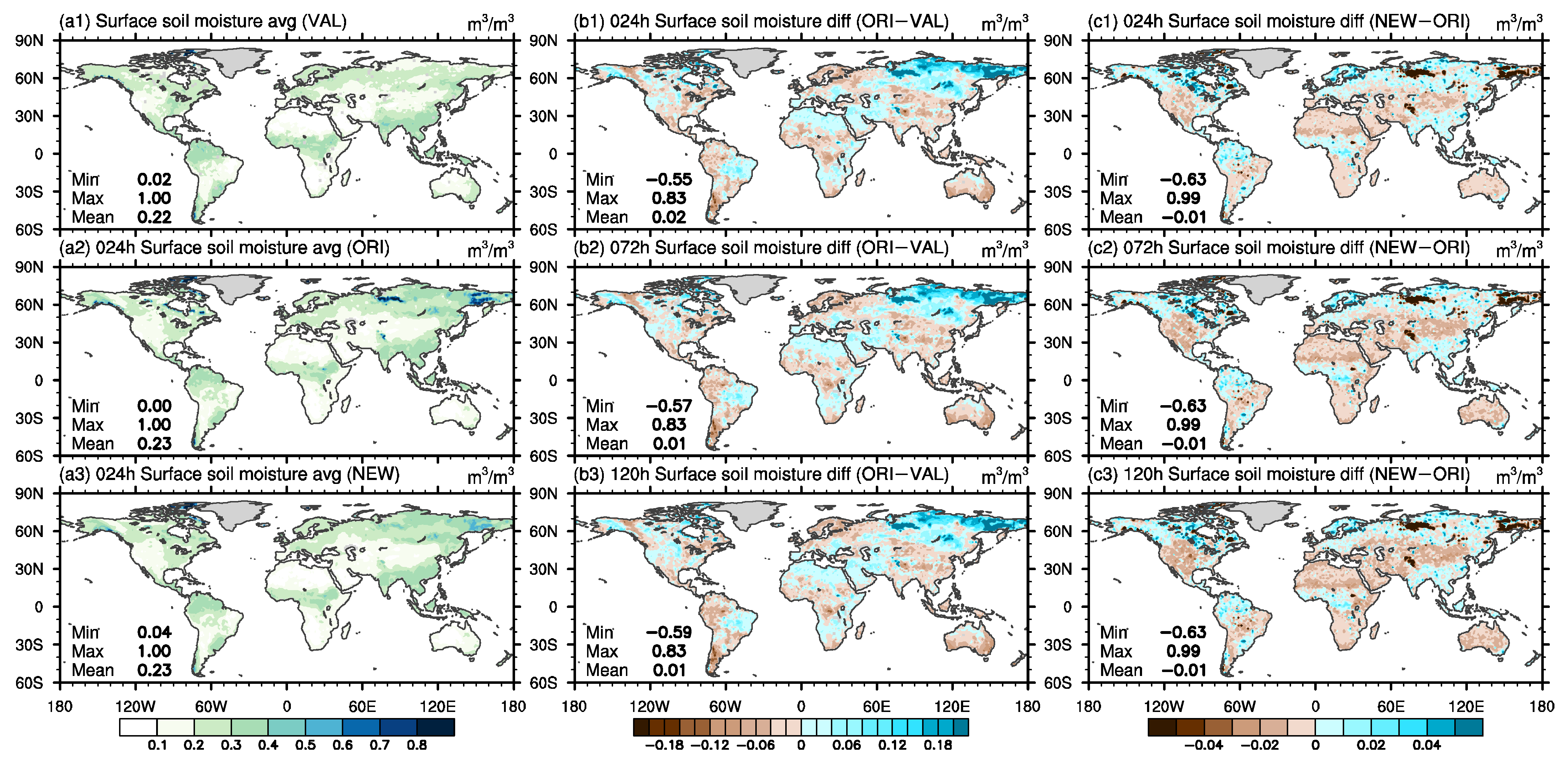
3.2.1. Surface Soil Moisture

The results derived from the 24 h forecast display a reasonable dry–wet distribution at a global scale (Figure 9(a1–a3)), with a relatively high soil moisture content over the tropical and mid-latitude region, and a relatively low soil moisture content over the desert and semi-arid regions. GRAPES_ORI shows an overestimation (+0.09 ${\mathrm{m}}^3$∙${\mathrm{m}}^{-3}$) of surface soil moisture over the arid and semi-arid regions such as western America, the Sahara Desert, and northeastern Eurasia, and an underestimation (−0.07 ${\mathrm{m}}^3$∙${\mathrm{m}}^{-3}$) over humid regions such as eastern America, central Africa, and Southeast Asia (Figure 9(b1–b3)). The prediction results from GRAPES_NEW correct these errors to some degree (Figure 9(c1–c3)), with about −0.03 ${\mathrm{m}}^3$∙${\mathrm{m}}^{-3}$ over the overestimation regions and about +0.02 ${\mathrm{m}}^3$∙${\mathrm{m}}^{-3}$ over the underestimation regions.

The RMSE of surface soil moisture between GRAPES prediction results and GLDAS in different regions is shown in

Table 9. RMSE of surface soil moisture between GRAPES forecast and GLDAS over different regions (units: ${\mathrm{m}}^3$∙${\mathrm{m}}^{-3}$).

Forecast Length (Units: h)	Global		Southern Hemisphere		Northern Hemisphere		East Asia
	ORI	NEW	ORI	NEW	ORI	NEW	ORI	NEW
24	0.0632	0.0562	0.0677	0.0593	0.0459	0.0444	0.0512	0.0480
48	0.0633	0.0563	0.0677	0.0592	0.0463	0.0450	0.0515	0.0489
72	0.0634	0.0565	0.0678	0.0593	0.0467	0.0458	0.0521	0.0498
96	0.0636	0.0568	0.0680	0.0595	0.0469	0.0463	0.0527	0.0506
120	0.0640	0.0573	0.0683	0.0599	0.0474	0.0470	0.0536	0.0516
144	0.0645	0.0578	0.0688	0.0604	0.0480	0.0478	0.0547	0.0528
168	0.0650	0.0583	0.0692	0.0608	0.0486	0.0487	0.0553	0.0534
192	0.0654	0.0589	0.0696	0.0613	0.0493	0.0496	0.0559	0.0543

. Firstly, RMSE increases slightly with longer forecasting hours in both GRAPES_ORI and GRAPES_NEW. Secondly, the RMSE of GRAPES_NEW decreases remarkably at most forecasting lengths over each individual region compared to GRAPES_ORI, with the global mean RMSE reduced by 10.6%. The growth in forecasting hours shows small impacts on the prediction skills. Overall, the GRAPES_NEW shows better performance on surface soil moisture prediction than that in GRAPES_ORI.

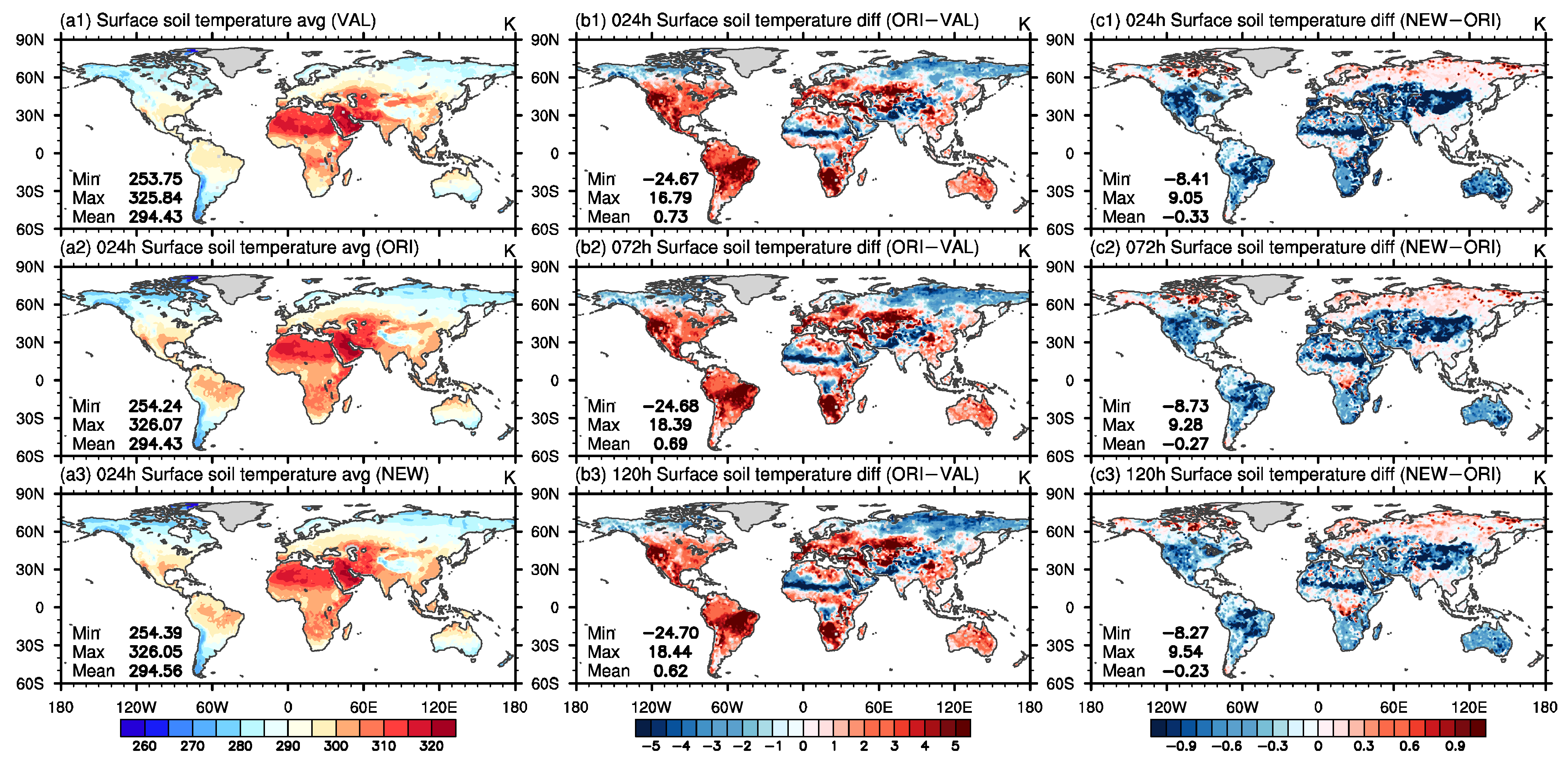
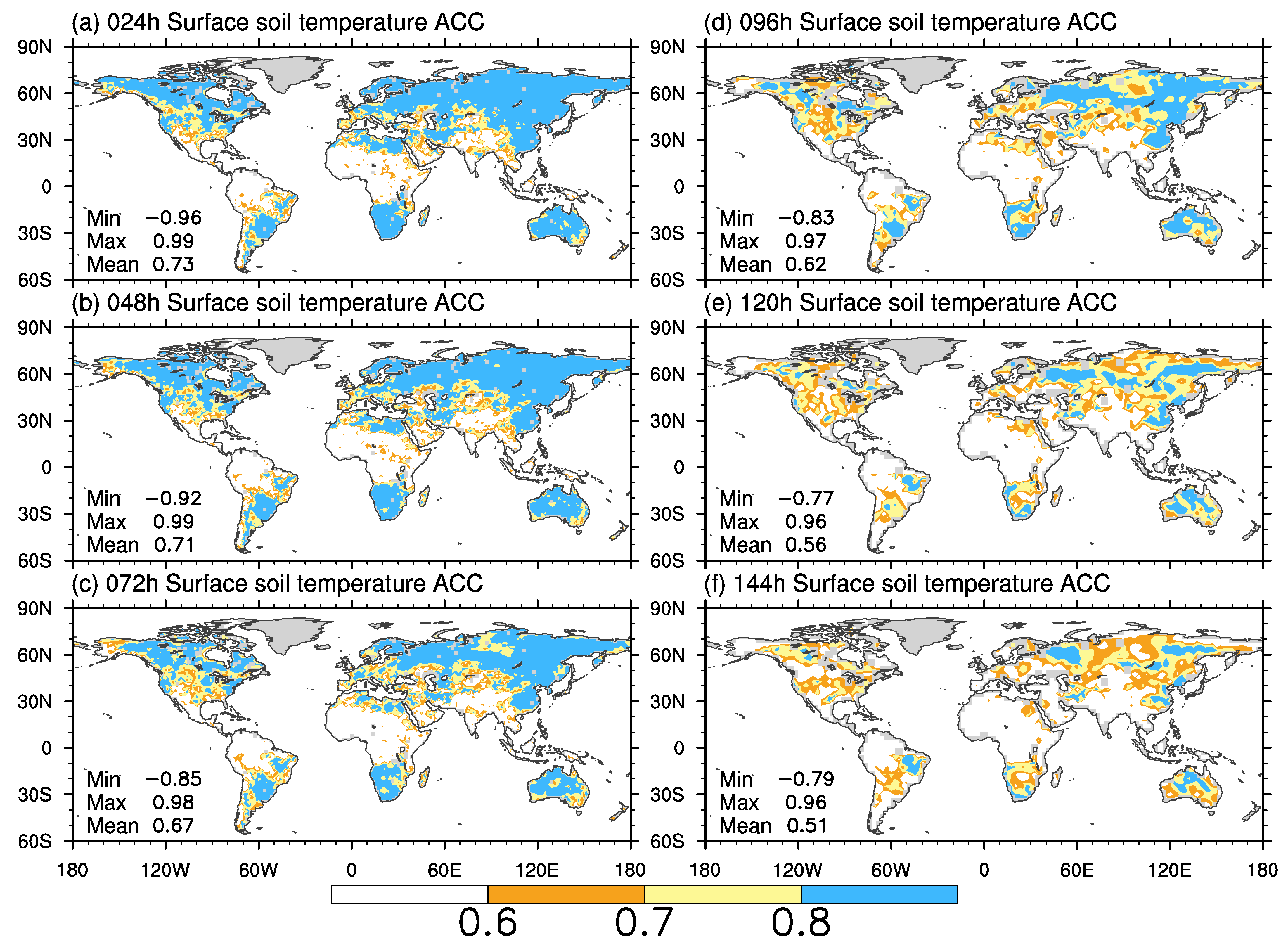
3.2.2. Surface Soil Temperature

As for surface soil temperature, the prediction skill of GRAPES_NEW also improves significantly.

Figure 10(a1–a3) shows that GRAPES can reproduce the spatial distribution of surface soil temperature at a relatively short prediction length. The distribution is quite like 2 m temperature, which indicates the close coupling between land and near-surface atmosphere. The prediction errors, however, display a strong overestimation over large areas, especially over the Americas, Africa, and central and eastern Eurasian continent (Figure 10(b1–b3)). The GRAPES_NEW shows great improvements on these overestimated regions with respect to GRAPES_ORI (Figure 10(c1–c3)).

The ACC spatial distribution of surface soil temperature (Figure 11) shows a good prediction skill within 3 days over the Eurasian continent, North America, southern Africa, and Australia. However, the ACC values decrease in most regions for the prediction lengths longer than 3 days.

Table 10. ACC of surface soil temperature between GRAPES forecast and GLDAS over different regions.

Forecast Length (Units: h)	Global		Southern Hemisphere		Northern Hemisphere		East Asia
	ORI	NEW	ORI	NEW	ORI	NEW	ORI	NEW
24	0.7171	0.7258	0.7301	0.7372	0.6672	0.6821	0.7624	0.7746
48	0.6969	0.7055	0.7082	0.7143	0.6534	0.6718	0.7286	0.7393
72	0.6581	0.6655	0.6648	0.6694	0.6323	0.6504	0.6819	0.6893
96	0.6125	0.6180	0.6139	0.6174	0.6072	0.6206	0.6337	0.6405
120	0.5549	0.5599	0.5538	0.5567	0.5590	0.5721	0.5803	0.5855
144	0.5072	0.5118	0.5012	0.5035	0.5302	0.5435	0.5287	0.5322
168	0.4573	0.4582	0.4483	0.4471	0.4921	0.5011	0.4917	0.4956
192	0.3948	0.3968	0.3918	0.3913	0.4062	0.4183	0.4416	0.4484

summarizes the area-averaged ACC values in different regions. We can see that even though the ACC values decrease rapidly with the increase in forecasting hours, the ACC values of each individual region still remain greater than 0.6 within 96 forecasting hours, which suggests that the surface soil temperature is predictable in 4 days at a global scale. Moreover, surface soil temperature over East Asia shows the highest ACC, followed by the Southern Hemisphere and the Northern Hemisphere. GRAPES_NEW gives higher ACC regional values than that of GRAPES_ORI. The results from

Table 11. RMSE of surface soil temperature between GRAPES forecast and GLDAS over different regions (units: K).

Forecast Length (Units: h)	Global		Southern Hemisphere		Northern Hemisphere		East Asia
	ORI	NEW	ORI	NEW	ORI	NEW	ORI	NEW
24	2.9772	2.8431	2.8367	2.7501	3.5198	3.2014	2.8377	2.9193
48	3.0622	2.8949	2.9525	2.8300	3.4857	3.1448	2.9930	2.9701
72	3.1799	3.0136	3.0972	2.9747	3.4993	3.1632	3.1539	3.0972
96	3.3104	3.1535	3.2610	3.1456	3.5012	3.1838	3.3218	3.2636
120	3.4578	3.3115	3.4331	3.3264	3.5528	3.2540	3.4944	3.4377
144	3.5887	3.4558	3.5834	3.4913	3.6088	3.3194	3.6020	3.5513
168	3.7313	3.6082	3.7395	3.6578	3.6997	3.4174	3.6751	3.6230
192	3.8565	3.7439	3.8659	3.7967	3.8203	3.5405	3.7628	3.7276

, which displays the RMSE of surface soil temperature between GRAPES and validation, also gives similar conclusions.

Overall, after updating CoLM schemes, GRAPES_NEW shows a smaller RMSE and a larger ACC on surface soil moisture and soil temperature than GRAPES_ORI.

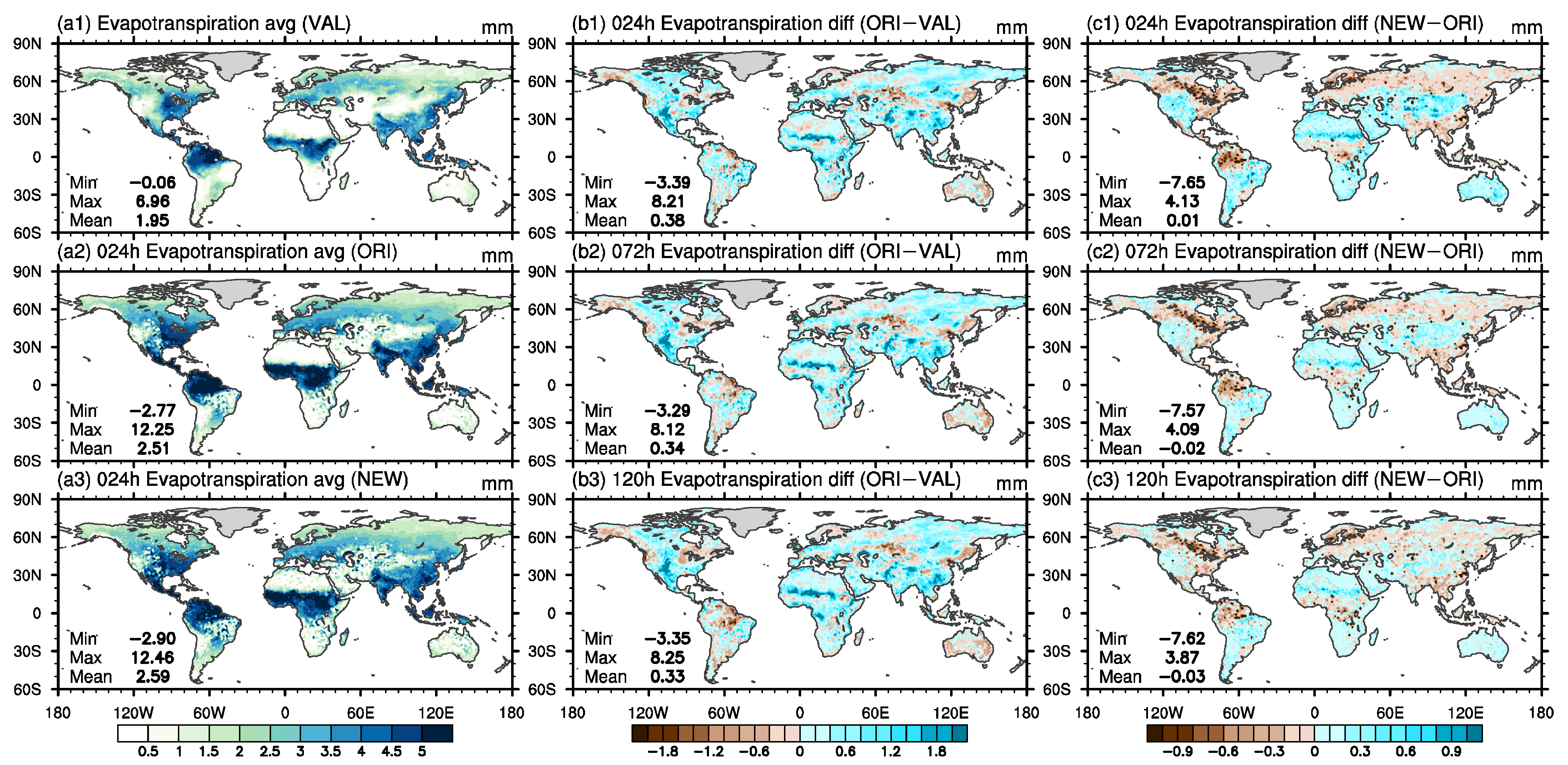
3.2.3. Evapotranspiration

The results from 24 h forecasts by GRAPES models show a similar distribution and magnitude with validation (Figure 12(a1–a3)), with higher evapotranspiration over eastern North America, tropical Africa, and South Asia, and lower evapotranspiration over the desert and semi-arid region. GRAPES_ORI (2.51 mm) and GRAPES_NEW (2.59 mm) tend to overestimate the evapotranspiration on the global mean value with respect to GLDAS (1.95 mm). The spatial distribution of overestimation in GRAPES_ORI is shown in Figure 12(b1 –b3). The prediction error does not change significantly with the increase in forecasting hours. Results from GRAPES_NEW show limited changes, but with notable improvements over humid areas such as the Amazon Rain Forest, tropical Africa, South Asia, and northern Eurasia continent (Figure 12(c1–c3)), which is consistent with the results found by Li et al. [12] which claimed that the surface latent heat flux has been corrected over the tropical Africa and Amazon Rain Forest in CoLM2014 when compared to CoLM2005.

We further calculate the area-averaged ACC (not shown) and RMSE (

Table 12. RMSE of 24 h net evapotranspiration between GRAPES forecast and GLDAS in different regions (units: mm).

Forecast Length (Units: h)	Global		Southern Hemisphere		Northern Hemisphere		East Asia
	ORI	NEW	ORI	NEW	ORI	NEW	ORI	NEW
24	2.9772	2.8431	2.8367	2.7501	3.5198	3.2014	2.8377	2.9193
48	3.0622	2.8949	2.9525	2.8300	3.4857	3.1448	2.9930	2.9701
72	3.1799	3.0136	3.0972	2.9747	3.4993	3.1632	3.1539	3.0972
96	3.3104	3.1535	3.2610	3.1456	3.5012	3.1838	3.3218	3.2636
120	3.4578	3.3115	3.4331	3.3264	3.5528	3.2540	3.4944	3.4377
144	3.5887	3.4558	3.5834	3.4913	3.6088	3.3194	3.6020	3.5513
168	3.7313	3.6082	3.7395	3.6578	3.6997	3.4174	3.6751	3.6230
192	3.8565	3.7439	3.8659	3.7967	3.8203	3.5405	3.7628	3.7276

) of GRAPES_ORI and GRAPES_NEW in different regions. They share a same conclusion that GRAPES_NEW has advantages on the prediction skill of evapotranspiration relative to GRAPES_ORI.

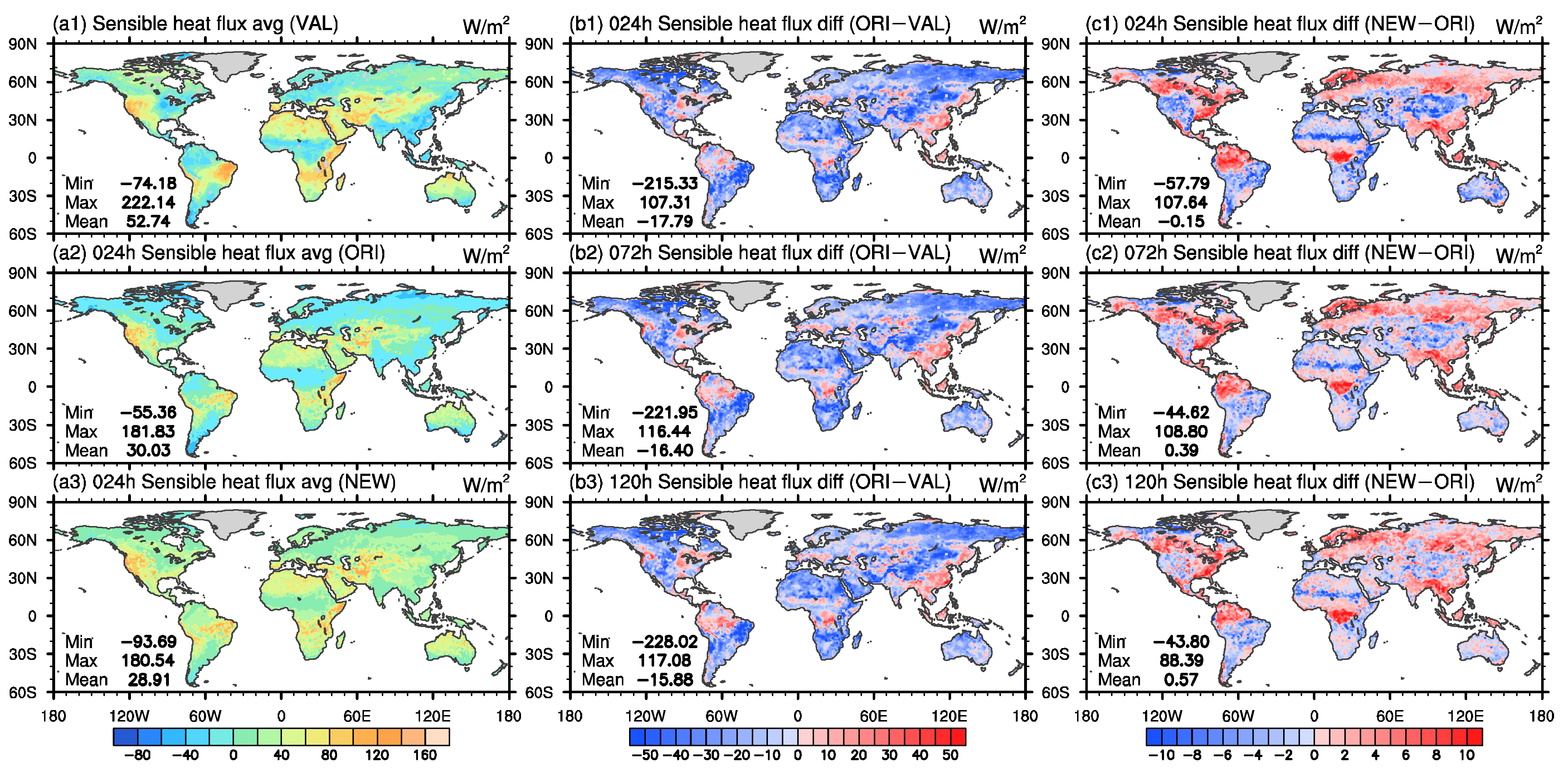
3.2.4. Sensible Heat Flux

The spatial distribution of 24 h forecasted sensible heat flux from GRAPES is similar to that from the validation (Figure 13(a1–a3)), with the high-value areas located in arid and semi-arid regions and low-value areas located in humid regions. GRAPES_ORI shows overestimated predictions over East China and underestimated predictions over the Middle East, Tibetan Plateau, northern America, and northern Eurasia continent (Figure 13(b1–b3)). GRAPES_NEW has corrected the underestimation of surface sensible heat flux in GRAPES_ORI, resulting in a closer result with validation (Figure 13(c1–c3)).

We also analyzed the areal mean ACC in different regions for multiple forecasting hours in both GRAPES_ORI and GRAPES_NEW (not shown). It is indicated that the Southern Hemisphere displays the best performances compared to the Northern Hemisphere and East Asia. In addition, GRAPES_NEW has a better performance in the prediction of surface sensible heat flux than that in GRAPES_ORI.

In conclusion, after updating CoLM schemes, the prediction skills of GRAPES have improved with respect to both atmospheric variables and land fields. It is noted that GRAPES with updated schemes still has systematic biases, which inspires us for further studies.

4. Conclusions

This study evaluates the performance of GRAPES coupled with the updated schemes of CoLM. We conducted two experiments. One (GRAPES_ORI) is GRAPES coupled with the older version of CoLM (CoLM2005), and the other (GRAPES_NEW) is GRAPES coupled with the newer version of CoLM (CoLM2014). Each experiment ran from 20 July to 1 September 2016, and validation datasets covered from 27 July to 1 September 2016. For each day during the validation period, we obtained forecast results from 1 day to 8 days. Based on these data, we evaluated the forecast results of some key atmospheric variables and land variables at different forecasting lengths and various regions, and the conclusions are as follows:

For atmospheric variables, both GRAPES_ORI and GRAPES_NEW can well reproduce their spatial patterns and magnitude for 24 h forecasts. The effective predictable lengths for most variables are up to 3 days at a global scale and can reach up to 6 days for parts of regions. The H500 and H850 are predictable for 6 days. Moreover, GRAPES_NEW has a better performance on the prediction skill of each individual variable than GRAPES_ORI by analyzing the spatial distribution of ACC and area-averaged ACC values and RMSE at different regions.

For land variables, we evaluated the prediction skill on surface soil moisture and soil temperature, evapotranspiration, and sensible heat flux. Both GRAPES_ORI and GRAPES_NEW can reproduce their spatial patterns and magnitude compared to the corresponding validation data. Furthermore, the GRAPES_NEW has greater improvements for predictions of land variables than atmospheric variables when compared with GRAPES_ORI, especially for the surface soil moisture and soil temperature, which could be attributed to the updated schemes of hydrological processes in CoLM.

Furthermore, the improvement of GRAPES_NEW in eastern Asia is larger than that of other regions, especially for the improvement of the geopotential height field, precipitation, near-surface wind and temperature, and surface soil moisture and temperature, which indicate a great potential of GRAPES_NEW for the weather forecast in eastern Asia.

Though the improvements are limited, GRAPES_NEW shows better performance on prediction skills in both atmospheric variables and land variables than that of GRAPES_ORI. However, there still exist systematic biases in both GRAPES_NEW and GRAPES_ORI, such as the overestimation of surface sensible heat flux over the Congo Rain Forest and the underestimation of evapotranspiration over the Great Lakes. In the future, more parameterization schemes of land processes in GRAPES should be added or updated for a better performance of the whole coupling model.

References

1. Dai, Y. Issues in Research and Development of Land Surface Process Model. Trans. Atmos. Sci. 2020, 43, 33–38. [Google Scholar] [CrossRef]
2. Zhuang, Z.; Xue, J.; Li, X.; Zhang, L. Estimation of Model Error for the Global GRAPES Model. Chin. J. Atmos. Sci. 2010, 34, 591–598. [Google Scholar] [CrossRef]
3. Tong, L.; Peng, X.; Fan, G.; Chang, J. Error Evaluation and Correction for GRAPES Global Forecasts. Chin. J. Atmos. Sci. 2017, 41, 333–344. [Google Scholar] [CrossRef]
4. Yang, X.; Shen, Y.; Xu, G. The Impacts of Radiation Schemes on the GRAPES Global Model. Chin. J. Atmos. Sci. 2009, 33, 593–599. [Google Scholar] [CrossRef]
5. Liu, K.; Chen, Q.; Sun, J. Modification of Cumulus Convection and Planetary Boundary Layer Schemes in the GRAPES Global Model. J. Meteorol. Res. 2015, 29, 806–822. [Google Scholar] [CrossRef]
6. Xu, D.; Chen, D. A Vertical Second-Order Difference Scheme for Non-uniformly Distributed Layers and Its Application in GRAPES Model. Chin. J. Atmos. Sci. 2020, 44, 975–983. [Google Scholar] [CrossRef]
7. Yang, J.; Shen, X. The Construction of SCM in GRAPES and Its Applications in Two Field Experiment Simulations. Adv. Atmos. Sci. 2011, 28, 534–550. [Google Scholar] [CrossRef]
8. Shen, X.; Su, Y.; Hu, J.; Wang, J.; Sun, J.; Xue, J.; Han, W.; Zhang, H.; Lu, H.; Zhang, H.; et al. Development and Operation Transformation of GRAPES Global Middle-Range Forecast System. J. Appl. Meteorol. Sci. 2017, 28, 1–10. [Google Scholar] [CrossRef]
9. Dai, Y.; Dickinson, R.E.; Wang, Y.-P. A Two-Big-Leaf Model for Canopy Temperature, Photosynthesis, and Stomatal Conductance. J. Clim. 2004, 17, 2281–2299. [Google Scholar] [CrossRef]
10. Dai, Y.; Zeng, X.; Dickinson, R.E.; Baker, I.; Bonan, G.B.; Bosilovich, M.G.; Denning, A.S.; Dirmeyer, P.A.; Houser, P.R.; Niu, G.; et al. The Common Land Model. Bull. Am. Meteorol. Soc. 2003, 84, 1013–1024. [Google Scholar] [CrossRef] [Green Version]
11. Dai, Y.; Yuan, H.; Shangguan, W.; Zhang, S.-P.; Wei, N.; Lu, X.; Liu, S.; Wei, Z.; Zhang, S.-L.; Li, L. The Common Land Model (CoLM) Version 2014. Available online: http://globalchange.bnu.edu.cn/research/models (accessed on 20 July 2020).
12. Li, C.; Lu, H.; Yang, K.; Wright, J.S.; Yu, L.; Chen, Y.; Huang, X.; Xu, S. Evaluation of the Common Land Model (CoLM) from the Perspective of Water and Energy Budget Simulation: Towards Inclusion in CMIP6. Atmosphere 2017, 8, 141. [Google Scholar] [CrossRef] [Green Version]
13. Chen, D.; Shen, X. Recent Progress on GRAPES Research and Application. J. Appl. Meteorol. Sci. 2006, 17, 773–777. [Google Scholar]
14. Huang, L.; Chen, D.; Deng, L.; Xu, Z.; Yu, F.; Jiang, Y.; Zhou, F. Main Technical Improvements of GRAPES_Meso v4.0 and Verification. J. Appl. Meteorol. Sci. 2017, 28, 25–37. [Google Scholar] [CrossRef]
15. Wu, X.; Jin, Z.; Huang, L.; Chen, D. The Software Framework and Application of GRAPES Model. J. Appl. Meteorol. Sci. 2005, 16, 539–546. [Google Scholar]
16. Dickinson, E.; Henderson-Sellers, A.; Kennedy, J. Biosphere-Atmosphere Transfer Scheme (BATS) Version 1e as Coupled to the NCAR Community Climate Model; NCAR Technical Note; National Center for Atmospheric Research (NCAR): Boulder, CO, USA, 1993. [Google Scholar] [CrossRef]
17. Dai, Y.; Zeng, Q. A Land Surface Model (IAP94) for Climate Studies Part I: Formulation and Validation in Off-line Experiment. Adv. Atmos. Sci. 1997, 14, 433–460. [Google Scholar] [CrossRef]
18. Bonan, G.B. A Land Surface Model (LSM Version 1.0) for Ecological, Hydrological, and Atmospheric Studies: Technical Description and User’ s Guide; NCAR Technical Note; National Center for Atmospheric Research (NCAR): Boulder, CO, USA, 1996. [Google Scholar]
19. Zhu, J.; Zeng, X.; Zhang, M.; Dai, Y.; Ji, D.; Li, F.; Zhang, Q.; Zhang, H.; Song, X. Evaluation of the New Dynamic Global Vegetation Model in CAS-ESM. Adv. Atmos. Sci. 2018, 35, 659–670. [Google Scholar] [CrossRef]
20. Ji, D.; Wang, L.; Feng, J.; Wu, Q.; Cheng, H.; Zhang, Q.; Yang, J.; Dong, W.; Dai, Y.; Gong, D.; et al. Description and Basic Evaluation of BNU-ESM Version 1. Geosci. Model Dev. Discuss. 2014, 7, 1601–1647. [Google Scholar] [CrossRef] [Green Version]
21. Liang, X.-Z.; Xu, M.; Yuan, X.; Ling, T.; Choi, H.I.; Zhang, F.; Chen, L.; Liu, S.; Su, S.; Qiao, F.; et al. Regional Climate-Weather Research and Forecasting Model. Bull. Am. Meteorol. Soc. 2012, 93, 1363–1387. [Google Scholar] [CrossRef]
22. Shangguan, W.; Dai, Y.; Duan, Q.; Liu, B.; Yuan, H. A Global Soil Data Set for Earth System Modeling. J. Adv. Model. Earth Syst. 2014, 6, 249–263. [Google Scholar] [CrossRef]
23. Dai, Y.; Shangguan, W.; Wei, N.; Xin, Q.; Yuan, H.; Zhang, S.; Liu, S.; Lu, X.; Wang, D.; Yan, F. A Review of the Global Soil Property Maps for Earth System Models. Soil 2019, 5, 137–158. [Google Scholar] [CrossRef] [Green Version]
24. Cosby, B.J.; Hornberger, G.M.; Clapp, R.B.; Ginn, T.R. A Statistical Exploration of the Relationships of Soil Moisture Characteristics to the Physical Properties of Soils. Water Resour. Res. 1984, 20, 682–690. [Google Scholar] [CrossRef] [Green Version]
25. Niu, G.Y.; Yang, Z.L.; Dickinson, R.E.; Gulden, L.E. A Simple TOPMODEL-Based Runoff Parameterization (SIMTOP) for Use in Global Climate Models. J. Geophys. Res. Atmos. 2005, 110, D21106. [Google Scholar] [CrossRef] [Green Version]
26. Beven, K.J.; Kirkby, M.J. A Physically Based, Variable Contributing Area Model of Basin Hydrology. Hydrol. Sci. Bull. 1979, 24, 43–69. [Google Scholar] [CrossRef] [Green Version]
27. Clapp, R.B.; Hornberger, G.M. Empirical Equations for Some Soil Hydraulic Properties. Water Resour. Res. 1978, 14, 601–604. [Google Scholar] [CrossRef] [Green Version]
28. Bonan, G.B. Sensitivity of a GCM Simulation to Inclusion of Inland Water Surfaces. J. Clim. 1995, 8, 2691–2704. [Google Scholar] [CrossRef]
29. Hostetler, S.W.; Bartlein, P.J. Simulation of Lake Evaporation with Application to Modeling Lake Level Variations of Harney-Malheur Lake, Oregon. Water Resour. Res. 1990, 26, 2603–2612. [Google Scholar] [CrossRef]
30. Henderson-Sellers, B. New Formulation of Eddy Diffusion Thermocline Models. Appl. Math. Model. 1985, 9, 441–446. [Google Scholar] [CrossRef]
31. Hostetler, S.W.; Bates, G.T.; Giorgi, F. Interactive Coupling of a Lake Thermal Model with a Regional Climate Model. J. Geophys. Res. Atmos. 1993, 98, 5045–5057. [Google Scholar] [CrossRef]
32. Hostetler, S.W.; Giorgi, F.; Bates, G.T.; Bartlein, P.J. Lake-Atmosphere Feedbacks Associated with Paleolakes Bonneville and Lahontan. Science 1994, 263, 665–668. [Google Scholar] [CrossRef]
33. Dai, Y.; Wei, N.; Huang, A.; Zhu, S.; Shangguan, W.; Yuan, H.; Zhang, S.; Liu, S. The Lake Scheme of the Common Land Model and Its Performance Evaluation. Chin. Sci. Bull. 2018, 63, 3002–3021. [Google Scholar] [CrossRef]
34. Kalnay, E.; Kanamitsu, M.; Kistler, R.; Collins, W.; Deaven, D.; Gandin, L.; Iredell, M.; Saha, S.; White, G.; Woollen, J.; et al. The NCEP/NCAR 40-Year Reanalysis Project. Bull. Am. Meteorol. Soc. 1996, 77, 437–472. [Google Scholar] [CrossRef] [Green Version]
35. Ma, Z.; Zhao, C.; Gong, J.; Zhang, J.; Li, Z.; Sun, J.; Liu, Y.; Chen, J.; Jiang, Q. Spin-up Characteristics with Three Types of Initial Fields and the Restart Effects on Forecast Accuracy in the GRAPES Global Forecast System. Geosci. Model Dev. 2021, 14, 205–221. [Google Scholar] [CrossRef]
36. Hong, S.-Y.; Kim, J.-H.; Lim, J.; Dudhia, J. The WRF Single-Moment 6-Class Microphysics Scheme (WSM6). J. Korean Meteorol. Soc. 2006, 42, 129–151. [Google Scholar]
37. Arakawa, A.; Schubert, W.H. Interaction of a Cumulus Cloud Ensemble with the Large-Scale Environment, Part I. J. Atmos. Sci. 1974, 31, 674–701. [Google Scholar] [CrossRef] [Green Version]
38. Han, J.; Pan, H.L. Revision of Convection and Vertical Diffusion Schemes in the NCEP Global Forecast System. Wea. Forecast. 2011, 26, 520–533. [Google Scholar] [CrossRef]
39. Mlawer, E.J.; Taubman, S.J.; Brown, P.D.; Iacono, M.J.; Clough, S.A. Radiative Transfer for Inhomogeneous Atmospheres: RRTM, a Validated Correlated-k Model for the Longwave. J. Geophys. Res. Atmos. 1997, 102, 16663–16682. [Google Scholar] [CrossRef] [Green Version]
40. Iacono, M.J.; Delamere, J.S.; Mlawer, E.J.; Shephard, M.W.; Clough, S.A.; Collins, W.D. Radiative Forcing by Long-Lived Greenhouse Gases: Calculations with the AER Radiative Transfer Models. J. Geophys. Res. Atmos. 2008, 113, D13103. [Google Scholar] [CrossRef]
41. Hong, S.-Y.; Pan, H.-L. Nonlocal Boundary Layer Vertical Diffusion in a Medium-Range Forecast Model. Mon. Wea. Rev. 1996, 124, 2322–2339. [Google Scholar] [CrossRef] [Green Version]
42. Hersbach, H.; Bell, B.; Berrisford, P.; Hirahara, S.; Horányi, A.; Muñoz-Sabater, J.; Nicolas, J.; Peubey, C.; Radu, R.; Schepers, D.; et al. The ERA5 Global Reanalysis. Quart. J. Roy. Meteorol. Soc. 2020, 146, 1999–2049. [Google Scholar] [CrossRef]
43. Huffman, G.J.; Bolvin, D.T.; Braithwaite, D.; Hsu, K.; Joyce, R.; Kidd, C.; Nelkin, E.J.; Sorooshian, S.; Tan, J.; Xie, P. NASA Global Precipitation Measurement (GPM) Integrated Multi-SatellitE Retrievals for GPM (IMERG); Algorithm Theoretical Basis Document (ATBD) Version 06; NASA Goddard Space Flight Center (GSFC): Greenbelt, MD, USA, 2019. [Google Scholar]
44. Skofronick-Jackson, G.; Kirschbaum, D.; Petersen, W.; Huffman, G.; Kidd, C.; Stocker, E.; Kakar, R. The Global Precipitation Measurement (GPM) Mission’s Scientific Achievements and Societal Contributions: Reviewing Four Years of Advanced Rain and Snow Observations. Quart. J. Roy. Meteorol. Soc. 2018, 144, 27–48. [Google Scholar] [CrossRef] [Green Version]
45. Rodell, M.; Houser, P.R.; Jambor, U.; Gottschalck, J.; Mitchell, K.; Meng, C.J.; Arsenault, K.; Cosgrove, B.; Radakovich, J.; Bosilovich, M.; et al. The Global Land Data Assimilation System. Bull. Am. Meteorol. Soc. 2004, 85, 381–394. [Google Scholar] [CrossRef] [Green Version]
46. Rui, H.; Beaudoing, H.; Loeser, C. README Document for NASA GLDAS Version 2 Data Products; README Document; NASA Goddard Space Flight Center (GSFC): Greenbelt, MD, USA, 2021. [Google Scholar]
47. Spennemann, P.C.; Rivera, J.A.; Celeste Saulo, A.; Penalba, O.C. A Comparison of GLDAS Soil Moisture Anomalies against Standardized Precipitation Index and Multisatellite Estimations over South America. J. Hydrometeorol. 2015, 16, 158–171. [Google Scholar] [CrossRef]
48. Zhang, S.; Liu, Y.; Cao, B.; Li, S. Soil Moisture-Precipitation Coupling and Trends in China, Based on GLDAS and CMIP5 Products. Clim. Environ. Res. 2016, 21, 188–196. [Google Scholar]
49. Hu, Z.; Chen, X.; Li, Y.; Zhou, Q.; Yin, G. Temporal and Spatial Variations of Soil Moisture over Xinjiang Based on Multiple GLDAS Datasets. Front. Earth Sci. 2021, 9, 654848. [Google Scholar] [CrossRef]
50. Deliry, S.I.; Pekkan, E.; Avdan, U. GIS-Based Water Budget Estimation of the Kizilirmak River Basin Using GLDAS-2.1 Noah and CLSM Models and Remote Sensing Observations. J. Indian Soc. Remote Sens. 2022, 1–19. [Google Scholar] [CrossRef]
51. Wang, Y.; Wang, S.; Song, W.; Yang, S. Application of GLDAS Data to the Potential Evapotranspiration Monitoring in Weihe River Basin. J. Arid Land Resour. Environ. 2013, 27, 53–58. [Google Scholar] [CrossRef]
52. Qi, W.; Liu, J.; Chen, D. Evaluations and Improvements of GLDAS2.0 and GLDAS2.1 Forcing Data’s Applicability for Basin Scale Hydrological Simulations in the Tibetan Plateau. J. Geophys. Res. Atmos. 2018, 123, 13128–13148. [Google Scholar] [CrossRef]
53. Wu, Z.; Feng, H.; He, H.; Zhou, J.; Zhang, Y. Evaluation of Soil Moisture Climatology and Anomaly Components Derived from ERA5-Land and GLDAS-2.1 in China. Water Resour. Manag. 2021, 35, 629–643. [Google Scholar] [CrossRef]
54. Liu, P.; Song, H.; Bao, W.; Li, J. Applicability Evaluation of CLDAS and GLDAS Soil Temperature Data in Shannxi Province. Meteorol. Sci. Technol. 2021, 49, 604–611. [Google Scholar]
55. Liu, S.; Wang, J.; Chen, Q.; Sun, J. The Main Characteristics of Forecast Deviation in Global Precipitation by GRAPES_GFS. Acta Meteorol. Sin. 2021, 79, 255–281. [Google Scholar] [CrossRef]
56. Murphy, A.H.; Epstein, E.S. Skill Scores and Correlation Coefficients in Model Verification. Mon. Wea. Rev. 1989, 117, 572–582. [Google Scholar] [CrossRef] [Green Version]
57. Zhi, X.; Wu, P.; Yu, J.; Mu, J.; Zhao, Q. Impact of Topographic Altitude Bias of the GFS Model on the 2 m Air Temperature Forecast. Trans. Atmos. Sci. 2019, 42, 652–659. [Google Scholar] [CrossRef]
58. Zhao, Y.; Li, X.; Peng, X. The Development of the GRAPES_YY Model and Its Performance Verification for Meiyu Frontal Precipitation Simulation. Acta Meteorol. Sin. 2020, 78, 623–635. [Google Scholar] [CrossRef]
59. Wang, Y.; Qian, H.; Song, J.J.; Jiao, M.Y. Verification of the T213 Global Spectral Model of China National Meteorology Center over the East-Asia Area. J. Geophys. Res. Atmos. 2008, 113, D10110. [Google Scholar] [CrossRef] [Green Version]
60. Lorenz, E.N. A Study of the Predictability of a 28-Variable Atmospheric Model. Tellus 1965, 17, 321–333. [Google Scholar] [CrossRef] [Green Version]
61. Palmer, W.C.; Allen, R.A. Note on the Accuracy of Forecasts Concerning the Rain Problem; US Weather Bureau: Silver Spring, MD, USA, 1949; p. 4. [Google Scholar]
62. Ebert, E.E. Methods for Verifying Satellite Precipitation Estimates. In Measuring Precipitation from Space; Levizzani, V., Bauer, P., Turk, F.J., Eds.; Springer: Dordrecht, The Netherlands, 2007; Volume 28, pp. 345–356. [Google Scholar]
63. Barnes, L.R.; Schultz, D.M.; Gruntfest, E.C.; Hayden, M.H.; Benight, C.C. CORRIGENDUM: False Alarm Rate or False Alarm Ratio? Wea. Forecast. 2009, 24, 1452–1454. [Google Scholar] [CrossRef] [Green Version]
64. Wang, Y.; Yan, Z. Effect of Different Verification Schemes on Precipitation Verification and Assessment Conclusion. Meteorol. Mon. 2007, 33, 53–61. [Google Scholar] [CrossRef]
65. Thompson, D.W.J.; Solomon, S. Interpretation of Recent Southern Hemisphere Climate Change. Science 2002, 296, 895–899. [Google Scholar] [CrossRef] [Green Version]
66. Kang, S.M.; Polvani, L.M.; Fyfe, J.C.; Sigmond, M. Impact of Polar Ozone Depletion on Subtropical Precipitation. Science 2011, 332, 951–954. [Google Scholar] [CrossRef] [Green Version]
67. Christidis, N.; Stott, P.A. Changes in the Geopotential Height at 500 HPa under the Influence of External Climatic Forcings. Geophys. Res. Lett. 2015, 42, 10798–10806. [Google Scholar] [CrossRef] [Green Version]
68. Krishnamurti, T.N.; Rajendran, K.; Vijaya Kumar, T.S.V.; Lord, S.; Toth, Z.; Zou, X.; Cocke, S.; Ahlquist, J.E.; Navon, I.M. Improved Skill for the Anomaly Correlation of Geopotential Heights at 500 HPa. Mon. Wea. Rev. 2003, 131, 1082–1102. [Google Scholar] [CrossRef] [Green Version]
69. Zhu, C.; Park, C.-K.; Lee, W.-S.; Yun, W.-T. Statistical Downscaling for Multi-Model Ensemble Prediction of Summer Monsoon Rainfall in the Asia-Pacific Region Using Geopotential Height Field. Adv. Atmos. Sci. 2008, 25, 867–884. [Google Scholar] [CrossRef]
70. Huang, Y.-Y.; Li, X.-F. The Interdecadal Variation of the Western Pacific Subtropical High as Measured by 500 hPa Eddy Geopotential Height. Atmos. Ocean. Sci. Lett. 2015, 8, 371–375. [Google Scholar] [CrossRef]
71. Pielke, R.A., Sr.; Avissar, R.; Raupach, M.; Dolman, A.J.; Zeng, X.; Denning, A.S. Interactions between the Atmosphere and Terrestrial Ecosystems: Influence on Weather and Climate. Glob. Chang. Biol. 1998, 4, 461–475. [Google Scholar] [CrossRef]
72. Tett, S.F.B.; Stott, P.A.; Allen, M.R.; Ingram, W.J.; Mitchell, J.F.B. Causes of Twentieth-Century Temperature Change near the Earth’s Surface. Nature 1999, 399, 569–572. [Google Scholar] [CrossRef]
73. Chen, X.; Shen, X.; Chen, H. Analysis of the Impact of Land Surface Process on Numerical Weather Prediction of Intensive Summer Rainfall over Huai River in 2007. J. Trop. Meteorol. 2010, 6, 667–679. [Google Scholar] [CrossRef]
74. Wu, J.; Li, Z.; Yan, P.; Yang, Y.; Bai, L.; Yang, J.; Peng, X. Quantitative Assessment of GRAPES Rainfall Forecast for Four Provinces of Northwest China. Meteorol. Mon. 2020, 46, 346–356. [Google Scholar] [CrossRef]
75. Betts, A.K. Land-Surface-Atmosphere Coupling in Observations and Models. J. Adv. Model. Earth Syst. 2009, 1, 18. [Google Scholar] [CrossRef]
76. Zhou, S.; Williams, A.P.; Lintner, B.R.; Berg, A.M.; Zhang, Y.; Keenan, T.F.; Cook, B.I.; Hagemann, S.; Seneviratne, S.I.; Gentine, P. Soil Moisture–Atmosphere Feedbacks Mitigate Declining Water Availability in Drylands. Nat. Clim. Chang. 2021, 11, 38–44. [Google Scholar] [CrossRef]
77. Wang, L.; Gong, J. Application of Two OI Land Surface Assimilation Techniques in GRAPES_Meso. Meteorol. Mon. 2018, 44, 857–868. [Google Scholar]
78. Manabe, S. Climate and the Ocean Circulation: I. The Atmospheric Circulation and the Hydrology of the Earth’s Surface. Mon. Wea. Rev. 1969, 97, 739–774. [Google Scholar] [CrossRef]
79. Wang, K.; Dickinson, R.E. A Review of Global Terrestrial Evapotranspiration: Observation, Modeling, Climatology, and Climatic Variability. Rev. Geophys. 2012, 50, RG2005. [Google Scholar] [CrossRef]
80. Dirmeyer, P.A.; Schlosser, C.A.; Brubaker, K.L. Precipitation, Recycling, and Land Memory: An Integrated Analysis. J. Hydrometeorol. 2009, 10, 278–288. [Google Scholar] [CrossRef]
81. Stefanidis, S.; Alexandridis, V. Precipitation and Potential Evapotranspiration Temporal Variability and Their Relationship in Two Forest Ecosystems in Greece. Hydrology 2021, 8, 160. [Google Scholar] [CrossRef]
Figure 1. How CoLM is coupled with other physical modules in GRAPES.
Land 11 00770 g001
Figure 2. Spatial distribution of time-averaged 500 hPa geopotential height (GPH) derived from (a1) ERA5 reanalysis dataset, (a2) GRAPES_ORI 24 h forecast results, and (a3) GRAPES_NEW 24 h forecast results; difference in time-averaged 500 hPa GPH between (b1) GRAPES_ORI 24 h forecast results, (b2) GRAPES_ORI 72 h forecast results, (b3) GRAPES_ORI 120 h forecast results and ERA5; difference in time-averaged 500 hPa GPH between (c1) GRAPES_NEW 24 h forecast results, (c2) GRAPES_NEW 72 h forecast results, (c3) GRAPES_NEW 120 h forecast results and GRAPES_ORI forecast results at the corresponding forecast lengths (units: gpm).
Land 11 00770 g002
Figure 3. Spatial distribution of anomaly correlation coefficient (ACC) of 500 hPa geopotential height between GRAPES_NEW (a) 24 h forecast; (b) 48 h forecast; (c) 72 h forecast; (d) 96 h forecast; (e) 120 h forecast; (f) 144 h forecast results and ERA5 at the corresponding time.
Land 11 00770 g003
Figure 4. Same as Figure 2, but for wind speed at 10 m (units: m∙ s 1 ).
Land 11 00770 g004
Figure 5. Same as Figure 3, but for ACC of wind speed at 10 m.
Land 11 00770 g005
Figure 6. Same as Figure 2, but for air temperature at 2 m (units: K).
Land 11 00770 g006
Figure 7. Same as Figure 3, but for ACC of air temperature at 2 m.
Land 11 00770 g007
Figure 8. Spatial distribution of time-averaged 24 h net precipitation derived from (a1) GPM dataset, (a2) GRAPES_ORI 24 h forecast results, and (a3) GRAPES_NEW 24 h forecast results; difference in time-averaged 24 h net precipitation between (b1) GRAPES_ORI 24 h forecast results, (b2) GRAPES_ORI 72 h forecast results, (b3) GRAPES_ORI 120 h forecast results and GPM at the corresponding time; difference in time-averaged 24 h net precipitation between (c1) GRAPES_NEW 24 h forecast results, (c2) GRAPES_NEW 72 h forecast results, (c3) GRAPES_NEW 120 h forecast results and GRAPES_ORI forecast results at the corresponding forecast lengths (units: mm).
Land 11 00770 g008
Figure 9. Spatial distribution of time-averaged surface soil moisture derived from (a1) GLDAS dataset, (a2) GRAPES_ORI 24 h forecast results, and (a3) GRAPES_NEW 24 h forecast results; difference in time-averaged surface soil moisture between (b1) GRAPES_ORI 24 h forecast results, (b2) GRAPES_ORI 72 h forecast results, (b3) GRAPES_ORI 120 h forecast results and GLDAS at the corresponding time; difference in time-averaged surface soil moisture between (c1) GRAPES_NEW 24 h forecast results, (c2) GRAPES_NEW 72 h forecast results, (c3) GRAPES_NEW 120 h forecast results and GRAPES_ORI forecast results at the corresponding forecast lengths (units: m 3 m 3 ).
Land 11 00770 g009
Figure 10. Same as Figure 9, but for surface soil temperature (Units: K).
Land 11 00770 g010
Figure 11. Spatial distribution of anomaly correlation coefficient (ACC) of surface soil temperature between GRAPES_NEW (a) 24 h forecast; (b) 48 h forecast; (c) 72 h forecast; (d) 96 h forecast; (e) 120 h forecast; (f) 144 h forecast results and GLDAS at the corresponding time.
Land 11 00770 g011
Figure 12. Same as Figure 9, but for 24 h net evapotranspiration (units: mm).
Land 11 00770 g012
Figure 13. Same as Figure 9, but for daily sensible heat flux (units: W∙ m 2 ).
Land 11 00770 g013