Article

Development of a Historical Multi-Year Land Cover Classification Incorporating Wildfire Effects

by
Katherine D. Morrison
and
Crystal A. Kolden
*
Department of Geography, University of Idaho, Moscow, ID 83844, USA
*
Author to whom correspondence should be addressed.
Submission received: 24 June 2014 / Revised: 11 September 2014 / Accepted: 22 September 2014 / Published: 26 September 2014

Abstract

:
Land cover change impacts ecosystem function across the globe. The use of land cover data is vital in the detection of these changes over time; however, most available land cover products, such as the National Land Cover Dataset (NLCD), are produced relatively infrequently. The most recent NLCD at the time of this research was produced in 2006 and does not adequately reflect the impact of land cover changes that have occurred since, including the occurrence of two large wildfires in 2008 in our study area. Therefore, there is a need for the classification of historical remotely sensed data, such as Landsat scenes, through replicable methods. While it is possible to collect field data coinciding with current or future Landsat acquisitions, it is impossible to retrospectively collect data for previous years; thus, fewer studies have focused on the classification of historical scenes. Using a single year of field reference and multi-year aerial photography data, we applied a simple decision tree classifier to accurately classify historic satellite data and produced maps of land cover to incorporate the effects of 2008 wildfires occurring between NLCD production dates. Overall accuracy ranged from 76 to 90 percent and was assessed using conventional error matrices.

1. Introduction

Land cover change impacts ecosystem function across the globe [1], and disturbance is a major driver of land cover change, which creates heterogeneous landscapes [2]. Large, infrequent disturbances, such as wildfires, are an essential component in many ecosystems, but have the potential to produce unexpected changes [3], especially when coupled with other impacts, such as a changing climate [4]. Wildfires burn with varying degrees of severity, which affects vegetation succession [5], land management efforts [6] and the potential for increased erosion and flooding [7]. In California, wildfire is a common driver of land cover change [8], and in the Big Sur region of the central California coast, the majority of area burned is the result of large infrequent fires controlled primarily by extreme weather [9]. These wildfires are of particular concern, because they can significantly alter vegetation in watersheds that transport sediment and nutrients to the adjacent nearshore oceanic environment [10]. In addition, these large coastal wildfire events have been shown to negatively impact marine coastal ecosystems and protected marine mammals [11,12,13]; these negative impacts are hypothesized to result from increases in the export of toxins, sediment and pollutants following land cover change [14,15,16,17].
Land cover data are vital in the detection of ecological change over time; these data are widely used in ecological applications. To accurately assess impacts to the nearshore environment, land cover data must accurately reflect any change caused by recent disturbance. The Multi-Resolution Land Characteristics Consortium (MLCR) National Land Cover Dataset (NLCD) is a commonly used land cover dataset [18,19,20,21]; however, at the time of this study, the most recent version of the NLCD was produced in 2006 (the 2011 NLCD was released in April 2014). Therefore, it did not reflect the impact of land cover changes that occurred between 2006 and 2011, such as two large 2008 wildfires that burned in the Big Sur region of the central California coast.
Detection of change in land cover requires multi-temporal assessments of land cover data. It has been common practice to analyze the difference between two scene dates to document change. However, time series approaches are increasingly common [22,23]. The Landsat multispectral data acquisition program, including Landsat Thematic Mapper (TM), Enhanced Thematic Mapper (ETM+) and Operational Land Imager (OLI), provides free, relatively high-resolution remotely sensed data from 1984 to the present that are widely used to study land cover change and disturbance at both regional and global scales.
One way to utilize a Landsat or other spectral data time series to understand change is to classify multispectral imagery, and a variety of classification methods have been developed [24]. A classification tree [25] uses recursive partitioning based on a variety of splitting rules to divide a dataset into categorical classes. Decision tree classifiers are simple, computationally efficient and transparent [26]. In addition, decision tree methods do not require statistical assumptions regarding distributions, are able to process large nonparametric datasets and use both continuous and categorical data [27].
A challenge in creating multi-temporal scene classification is the collection of high-quality field data for training and validation. Although it is possible to collect field data coinciding with current or future Landsat acquisitions, it is impossible to conduct field sampling to collect data for land cover classification of previous years and incredibly difficult and cost-prohibitive to collect field data over large areas. In such cases, it is possible to use other sources of information to create reference data, such as higher resolution aerial photographs [24,28,29]. Unfortunately, aerial photographs coinciding with satellite data acquisitions are not always common, and therefore, it becomes necessary to extrapolate the reference data over time [30].
Numerous studies have used decision tree, maximum likelihood, Fourier analysis and other methods to classify land cover for historic periods, either to detect change or assess trends [30,31]. Global scale land cover classifications have primarily utilized lower resolution data from the Advanced Very High Resolution Radiometer (AVHRR) or the Moderate-resolution Imaging Spectroradiometer (MODIS) in a time series, such that the phenological pattern contributes to the land cover classification [30], but data at that scale are not appropriate when incorporating the high-resolution effects of wildfire [32]. Higher resolution Landsat data are more difficult to develop annual classifications from, as cloud impacts and sensor failures can limit scene availability [33]. Our challenge in this study was to classify land cover over multiple sequential years (as required for the model that the land cover classifications would be utilize as inputs for) at a spatial resolution that would capture wildfire effects (i.e., Landsat), in complex terrain with diverse land cover that transitions rapidly between three primary life form strata (i.e., forest, shrub and grass). Furthermore, we needed to understand both overall accuracy and spatial accuracy, as the subsequent modelling effort produced spatially-explicit outputs that would have differing levels of error based on spatial accuracy. Our goal, therefore, was to develop a method for classifying a time series of Landsat data using a decision tree classifier developed with a single year of field observations. The success of the classification was then assessed using both the standard error matrix and a local representation of the error. Our objectives were to: (1) create a parsimonious decision tree that accurately classified historic remotely sensed data; and (2) produce maps of land cover from 2005 to 2012 for the Big Sur region that would incorporate the effects of the 2008 wildfires. The produced land cover dataset would subsequently be used in a later study to model nonpoint source pollutant transport from the Big Sur coastal watersheds to the nearshore environment [34].

2. Methods

2.1. Study Area

The study area boundary is formed by 15 adjacent watersheds covering 87,638 ha in the northern portion of the Los Padres National Forest (Figure 1) and extends approximately 109 km along the Santa Lucia Range south of Monterey Bay. The Santa Lucia Range rises steeply from sea level to just below 1800 m within a few km from the coast. The climate is Mediterranean with long, dry summers and warm, wet winters. Precipitation ranges from 65 cm annually near the coast to over 130 cm at higher elevations [35]. Temperature generally increases from north to south and with distance from the coast, with coastal mean monthly temperature ranging from 10 °C–13 °C in winter to 16 °C–18 °C in summer [9]. These weather and elevation gradients create a highly diverse ecosystem that has been identified as a global biodiversity “hotspot” [36]. The study area consists of three ecological zones, each including a number of vegetation types. The coastal plains and foothills include grasslands, coastal sage scrub, chaparral, oak forests and closed-cone pine forest. The lower montane zone includes a mixture of coastal sage scrub, chaparral and oak woodlands and forests. The upper montane zone primarily contains mixed broadleaf evergreen and coniferous forests [9].
Figure 1. The Big Sur region of the central California coast and the 2008 Basin Complex and Chalk Fires.
Land 03 01214 g001

2.2. Satellite and Ancillary Data

To classify land cover through time, the Surface Reflectance Climate Data Record (CDR) produced by the Landsat Ecosystem Disturbance Adaptive Processing System (LEDAPS) was used. Surface Reflectance CDR processes Landsat scenes to at-surface reflectance using the second simulation of the satellite signal in the solar spectrum (6S) radiative transfer model [37]. Seven CRD Landsat TM and two Landsat ETM+ scenes (Path 33/Row 34) were acquired. Cloud-free data were acquired for eight years from 2005 to 2012 within the months of July and August (Table 1). CRD Landsat data are Level-1 geometrically and terrain-corrected [37]. Landsat ETM+ imagery after 31 May 2003, was affected by the failure of the Scan Line Corrector, which causes “stripes” of missing data [38]. Because of the relative clarity of the atmosphere and the static nature of vegetation during the summer months over the study site, missing data on 19 July 2012, were filled from the closest and most cloud-free scene available from 3 July 2012.
The suite of potential predictor variables for creating the classification tree included Landsat Bands 1 through 5 and 7 from the TM and ETM+ sensors (Table 2). We also calculated several indices, such as the normalized differenced vegetation index (NDVI) [39,40], normalized burn ratio (NBR) [41] and band ratios 4/3 and 7/4. NDVI has been used in decision tree classifiers to discriminate differences in vegetation from non-vegetation cover [26]. NBR has not been widely used in decision-tree classifiers, but is used to classify fire effects on vegetation [41], as changes in near-infrared wavelengths indicate a change in green vegetation and biomass [42], whereas the shortwave infrared band is sensitive to soil and plant moisture [43], as well as burnt vegetation, ash and exposed soil [44]. Band ratios 4/3 and 7/4 were selected to highlight green vegetation or lack of green vegetation, respectively; they have been included in numerous prior land cover classification studies. We also used tasseled cap transformations of greenness (TCG), wetness (TCW) and brightness (TCB) [45], because of their ability to discriminate differences in vegetation cover in a prior decision tree classification [28]. Incorporation of variables that utilize the spatial information has been shown to increase the accuracy of remote sensing classification [46,47,48].
Table 1. The sensor name and date of acquisition of remotely sensed scenes. Two scenes were acquired in 2012 to fill data gaps associated with the scan-line corrector failure on Landsat ETM+.
SensorYearMonth/Day
Landsat TM2005July/8
2006July/11
2007July/14
2008August/1
2009July/19
2010August/23
2011July/25
Landsat ETM+2012July/19
2012July/3
Table 2. Spectral and ancillary input variables. Band numbers represent bands from the Landsat TM and ETM+sensors. Indices and transforms include the normalized differenced vegetation index (NDVI), normalized burn ratio (NBR), tasseled cap brightness (TCB), tasseled cap wetness (TCW) and tasseled cap greenness (TCG).
VariableDescription
Spectral
Band 1 (B1)0.45–0.52 µm TM, 0.45–0.515 µm ETM+
Band 2 (B2)0.52–0.60 µm TM, 0.525–0.605 µm ETM+
Band 3 (B3)0.63–0.69 µm TM, ETM+
Band 4 (B4)0.76–0.90 µm TM, 0.75–0.90 µm ETM+
Band 5 (B5)1.55–1.75 µm TM,ETM+
Band 7 (B7)2.09–2.35 µm TM, 2.09–2.35 µm ETM+
Low Band 13 × 3 Mean Filter of Band 1 reflectance
Low Band 23 × 3 Mean Filter of Band 2 reflectance
Low Band 33 × 3 Mean Filter of Band 3 reflectance
Low Band 43 × 3 Mean Filter of Band 4 reflectance
Low Band 53 × 3 Mean Filter of Band 5 reflectance
Low Band 73 × 3 Mean Filter of Band 7 reflectance
4/3 ratioB4/B3
7/4 ratioB7/B4
NDVI(B4 − B3)/(B4 + B3)
NBR(B7 − B4)/(B7 + B4)
TCB0.2043 × B1 + 0.4158 × B2 + 0.5524 × B3 + 0.5741 × B4 + 0.3124 × B5 + 0.2303 × B7
TCW0.0315 × B1 + 0.2021 × B2 + 0.3102 × B3 + 0.1594 × B4 − 0.6806 × B5 − 0.6109 × B7
TCG−0.1603 × B1 − 0.2819 × B2 − 0.4934 × B3 + 0.7940 × B4 − 0.0002 × B5 − 0.1446 × B7
Ancillary
AspectNorth, South, East, West Categories
SlopeDegrees
ElevationMeters
The spectral reflectance bands were smoothed using a mean low-pass 3 × 3 filter [49]. The purpose of this smoothing process is two-fold. First, we observed during our field work that the vegetation classes vary at a larger scale than the resolution of the data (i.e., patches are generally greater than 30 m × 30 m in size), and the filter smoothes out the spectral noise of an isolated vegetation anomaly (e.g., a single remnant pine tree in the middle of an extensive shrub patch). Second, the filter also removes the spectral noise associated with scattering from adjacent pixels, which is inherent in passive remote sensing [49].
To derive terrain variables, which have been shown to be useful in the classification of vegetation in southern California [50], two 1-arcsecond USGS Nation Elevation Dataset (NED) tiles were mosaicked and processed to produce elevation, aspect and slope. Aspect was converted to categorical data with four classes: north (316°–45°), east (46°–135°), south (136°–225°) and west (226°–315°).

2.3. Classification Scheme and Reference Data

Classification categories of forest, shrub and grass were chosen as broad classes to subsume all vegetation community types in the study area. Though both evergreen and mixed forest types are present in the study area, the two classes were combined, because of the small percentage of mixed forest and substantial confusion between the classes. Class definitions were based on those defined by the Multi-Resolution Land Characteristics Consortium (MLCR) National Land Cover Dataset (NLCD) [33] (Table 3).
Table 3. Land cover classes based on the descriptions used for the National Land Cover Dataset (NLCD).
Land-Cover ClassClass Description
ForestAreas dominated by trees generally greater than 5 m tall and greater than 20 percent of total vegetation cover; includes both evergreen forest, where canopy is never without foliage, and mixed forest, where neither deciduous nor evergreen species are greater than 75% of the total tree cover
ShrubAreas dominated by shrubs less than 5 m tall with shrub canopy typically greater than 20% of total vegetation; includes true shrubs, young trees in the early successional stage or foliage stunted from environmental conditions
GrassAreas dominated by graminoid or herbaceous vegetation, generally greater than 80% of the total vegetation; includes grazing
Training and validation reference data were collected in the field for the 2012 classification tree in November 2012. Each sample point was collected to represent a pixel in one of the three cover classes. At each point, vegetation was assessed as a pixel with a 30- by 30-m area. Due to rugged terrain and dense vegetation, much of the study area is inaccessible, so the location of field sampling points was limited to areas accessible by roads and trails. To increase the pool of reference points, increase the spatial distribution and better cover the three vegetation classes, reference data were also sampled by photointerpretation of a 2012 National Agriculture Imagery Program (NAIP) high-resolution aerial photograph on a dot grid over the study area. At each point, if an approximate 30- by 30-m area was a visually homogeneous patch it was recorded as one of the three classes. Unclear or heterogeneous patches were excluded. Photointerpretation yielded 360 reference points, while field collection produced 219 reference points, for a total of 579 reference points (Table 4). Reference points from 2012 were randomly divided into two separate subsets for training (75 percent) and validation (25 percent) of the 2012 classification.
High resolution aerial photos from NAIP were also available for 2005 and 2009 and were used to obtain validation data for these two years by photointerpretation from the same point grid. From this grid of points, 180 sites were identified for 2005 and 164 sites were identified for 2009. For the remaining years (2006–2008, 2010, 2011), persistent sites were used for validation. Persistent sites were defined as sites photointerpreted from NAIP in 2005, 2009 and 2012 outside of the area of the two 2008 fires for which the identified class did not change across those three years (i.e., the class was persistent). We specifically excluded sites from within the fire perimeters, because we could not rule out fire effects on these sites; most were burned in 2008 (i.e., not persistent) and even if they appeared persistent, there may have been a change in vegetation vigor associated with fire effects (e.g., an understory burn in the forested sites). There were 147 persistent sites identified used for validation of these years (Table 4).
Table 4. Summary of reference site data obtained for classification and accuracy assessment. Field data were collected in 2012. National Agriculture Imagery Program (NAIP) sources were photointerpreted from a point grid over the study area. Persistent sites consist of photointerpreted sites that remained constant in class between the 2005, 2009 and 2012 NAIP images. The 2012 sites were randomly divided into training (75 percent) and validation (25 percent); for all other years, all sites were used for validation of the year listed (either the year of the NAIP image or the persistent sites).
YearData SourceNumber of SitesUtility
2012Field; NAIP164; 270Training for 2012 classification
Field; NAIP55; 90Validation for 2012 classification
2009NAIP164Validation for 2009 classification
2005NAIP180Validation for 2005 classification
--Persistent Sites from NAIP147Validation for 2006, 2007, 2008, 2010 and 2011 classifications

2.4. Classification Tree

Because field data were collected in 2012, it was considered as the “base” classification year. A base year classification tree was developed for 2012 with 23 spectral and ancillary variables and reference training data collected in the field, as well as from high resolution aerial photographs also from 2012. The Idrisi Classification Tree Analysis (CTA) module with the gain ratio splitting algorithm option was used to develop the decision tree. Pruning is necessary to prevent the tree from over-fitting the data, which can lead to poor classification of the entire dataset [51]. Pruning levels of 1, 5 and 10 percent were all tested for their ability to produce the most parsimonious tree with the highest accuracy. The decision rules generated by the 2012 base tree were then applied to the Landsat scene for each of the seven preceding years (2005–2011), producing a classified map of land cover for each year for a total of eight classified land cover maps from 2005 to 2012.

2.5. Accuracy Assessment

We assessed classification accuracy using error matrices that provide the overall accuracy of the map, per class errors of commission and omission and the kappa statistic [52]. A global estimate of overall accuracy (provided by the error matrix) may not be appropriate for all areas of the map, especially in sub-regions [53]. Based on the methods from Comber et al. [53], a geographically weighted logistic regression was used to analyze how the classification accuracy varied across space. Because the presence or absence of a specific land cover class is binary, a logistic regression or logit model is used. Logistic models provide a probability ranging from 0 to 1, representing the correct prediction of a land cover class. When used in combination with geographically weighted regression (GWR) [54], this allows for the local assessment of correctly classified and incorrectly classified land cover to vary over space. The assumption that relationships vary across space required the use of a moving kernel, which only considers data within a specified window to obtain regression estimates. Data are weighed according to proximity to a point; data that are closer are weighted higher and, conversely, data that are further are weighted less [54]. The bandwidth is variable and is determined by a leave-one-out cross-validation method to select the optimal number of data points [53]. The results of the geographically weighted logistic regression provides the probability that the presence of the reference data is correctly identified by the classified data expressed as probabilities [53].

3. Results

3.1. Classification Tree

The classification tree for the 2012 data, which was achieved with a five percent pruning level, is shown in Figure 2. The decision tree analysis resulted in a simple tree that used only NDVI, tasseled cap greenness and the low pass filter of Band 7 out of the 23 input variables, using NDVI twice. At the first node, NDVI was used to identify grass. This was the only terminal node at which grass was assigned, indicating that the remainder of the classification tree nodes separated shrub from forest. At the second node, the low pass mean filter of Band 7 split forest into a terminal node. The second use of NDVI separated out a portion of the shrub points as having a lesser NDVI value, and the final node used tasseled cap greenness to separate the remaining shrub from forest.

3.2. Classification Accuracy

The 2012 classification produced a map (Figure 3) with a 90 percent overall accuracy and 0.84 kappa (Table 5). The overall accuracies for all years varied from 74 to 90 percent with the highest accuracy in 2012 and the lowest in 2011 (Table 5). Kappa values ranged from the highest of 0.84 in 2012 and lowest of 0.56 in 2011 (Table 5). Overall and per class accuracies and kappa values for each year are reported in Table 5.
Table 5. Error matrices for each year. The rows represent classified pixels, and columns represent the spatially corresponding validation sites. Omission error is the proportion of incorrectly classified validation sites. The commission error is the proportion of pixels incorrectly classified. Overall accuracy is the total number of correctly classified pixels divided by the total number of pixels. The Kappa statistic is a metric that accounts for the overall totals, as well as individual class accuracies.
ReferenceReference
Year 2005ForestShrubGrassTotalCommission ErrorYear 2009ForestShrubGrassTotalCommission Error
ClassifiedForest 70181890.21ClassifiedForest56230790.29
Shrub15481640.25Shrub7494600.18
Grass0918270.33Grass1420250.20
Total8575200.76OverallTotal6476240.76Overall
Omission Error0.180.360.100.59KappaOmission Error0.130.360.170.62Kappa
2006ForestShrubGrassTotalCommission Error2010ForestShrubGrassTotalCommission Error
Forest58141730.21Forest63100730.14
Shrub9398560.30Shrub 11441560.21
Grass0315180.17Grass0315180.17
Total6756240.76Overall Total7457160.83Overall
Omission Error0.130.300.380.61KappaOmission Error0.150.230.060.71Kappa
2007ForestShrubGrassTotalCommission Error2011ForestShrubGrassTotalCommission Error
Forest 47242730.36Forest59140730.19
Shrub 3467560.18Shrub16391560.30
Grass0117180.06Grass0711180.39
Total5071260.75OverallTotal7560120.74Overall
Omission Error0.060.350.350.60KappaOmission Error0.210.350.080.56Kappa
2008ForestShrubGrassTotalCommission Error2012ForestShrubGrassTotalCommission Error
Forest49240730.33Forest35130480.27
Shrub3494560.13Shrub1441460.04
Grass0117180.06Grass0050500.00
Total5274210.78OverallTotal3657510.90Overall
Omission Error0.060.340.190.65KappaOmission Error0.030.230.020.84Kappa
Figure 2. Classification tree developed for the 2012 base year that was applied to all years.
Land 03 01214 g002
Figure 3. Classification map produced from the 2012 Landsat data that had the highest overall accuracy.
Land 03 01214 g003
Accuracy associated with each class for 2012 is shown as minimum, median, maximum and first and third quartiles (Table 6). Following prior studies, the inter-quartile range (IQR) here is interpreted as a representative metric of spatial variation in accuracy; the larger the IQR value, the greater the spatial variation [53]. The class with the highest variability in 2012 was shrub cover (Figure 4). Quartiles are plotted as maps over the study area showing the spatial representation of the probabilities of correctly and incorrectly classified shrub cover from Table 6 (Figure 4). When the spatial map of probabilities are mapped along with reference data, the influence of the reference and classification points is apparent [53]. For example, the accuracy map for 2012 shrub (Figure 4) demonstrates that areas where many points agree have a higher probability of correct prediction, whereas areas of less probability coincide with more frequent misclassifications. Areas where there are no reference data are also shown as highly likely to be correctly predicted, as there is no error.
Figure 4. Maps of spatial distribution of accuracy for 2012 shrub cover. Values in the legend represent the probability of the presence of the correct class. Maps of agreement between the reference data and the classified map for 2012. Solid circles represent agreement in both data sets. Unfilled circles represent shrub points incorrectly classified as forest or grass (omission error). Crosses represent points incorrectly classified as shrub (commission error).
Land 03 01214 g004
Table 6. Quartiles for geographically weighted logistic regression representing the probability of the classification correctly predicting the 2012 reference data. Interquartile range (IQR) represents the variability in probability among pixels. 1st and 3rd quartiles (1st Q, 3rd Q) represent the 25th and 75th percentile probabilities.
YearClassMin1st QMedianMean3rd QMaxIQR
2012Forest0.840.880.910.910.931.000.045
Shrub0.600.850.900.890.931.000.082
Grass0.910.991.000.991.001.000.008

4. Discussion

The decision tree relied mainly on variables sensitive to vegetation characteristics. We were surprised that elevation was not chosen as a variable to distinguish between forest and shrub, because forests are found primarily along ridge tops at the highest elevations (pine forests) or along the bottom of river valleys at the lowest elevations (redwood forests), but the spectral signal was chosen as a more discriminating determinant. This is potentially because the three classes were well-distributed spatially across all topographic variables, due to the strong moisture gradient from north to south [9,55]. NDVI, sensitive to plant greenness and biomass, was used at the first node to identify grass that at the time was senesced, producing significantly lower NDVI values than shrub or forest cover. The use of tasseled cap greenness, representing vegetation greenness and NDVI, were used to identify forest from shrub based on spectral differences in vegetation and differences in biomass. The incorporation of spatial dependence by using a mean filter of Band 7 (sensitive to vegetation moisture) effectively split forest from shrub. Overall accuracy of the 2012 base classification was 90 percent with a kappa of 0.84, where 85 percent is suggested to be a baseline for overall accuracy [56], and a kappa value of greater than 0.80 indicates high agreement between a classified map and reference data [49]. However, once the 2012 decision tree was applied to the seven years of Landsat data, the overall accuracies fell, ranging from 75 to 83 percent, with kappa values ranging from 0.56 to 0.71. Low kappa values were a result of confusion among the classes, especially between forest and shrub.
Because of its spectral dissimilarity from other classes, particularly during the mid-to-late summer when it has senesced, grass produced the highest accuracies. Some inaccuracies in grass can be attributed to a few small areas, where pasture land remains green from irrigation and the presence of nonnative species that retain their greenness late into the summer, and is classified as shrub. Shrub and forest classes consistently produced the lowest accuracies. Much of the vegetation in the study area is evergreen (both forest and shrub), and shrub cover in areas can be visually difficult to differentiate from forest; thus, the highest confusion was between these classes. In particular, patches of the evergreen coast live oak forest grow extensively in grasslands and savannas [9] and can be difficult to differentiate from and are often classified as shrub.
In land cover classification with relatively high accuracy, it may not be necessary to spatially map local accuracy. However, when a land cover classification results in low accuracy or has problematic classes of poor accuracy, a spatial representation could be beneficial. Information from the maps of accuracy can be used to understand the causes of its variation [
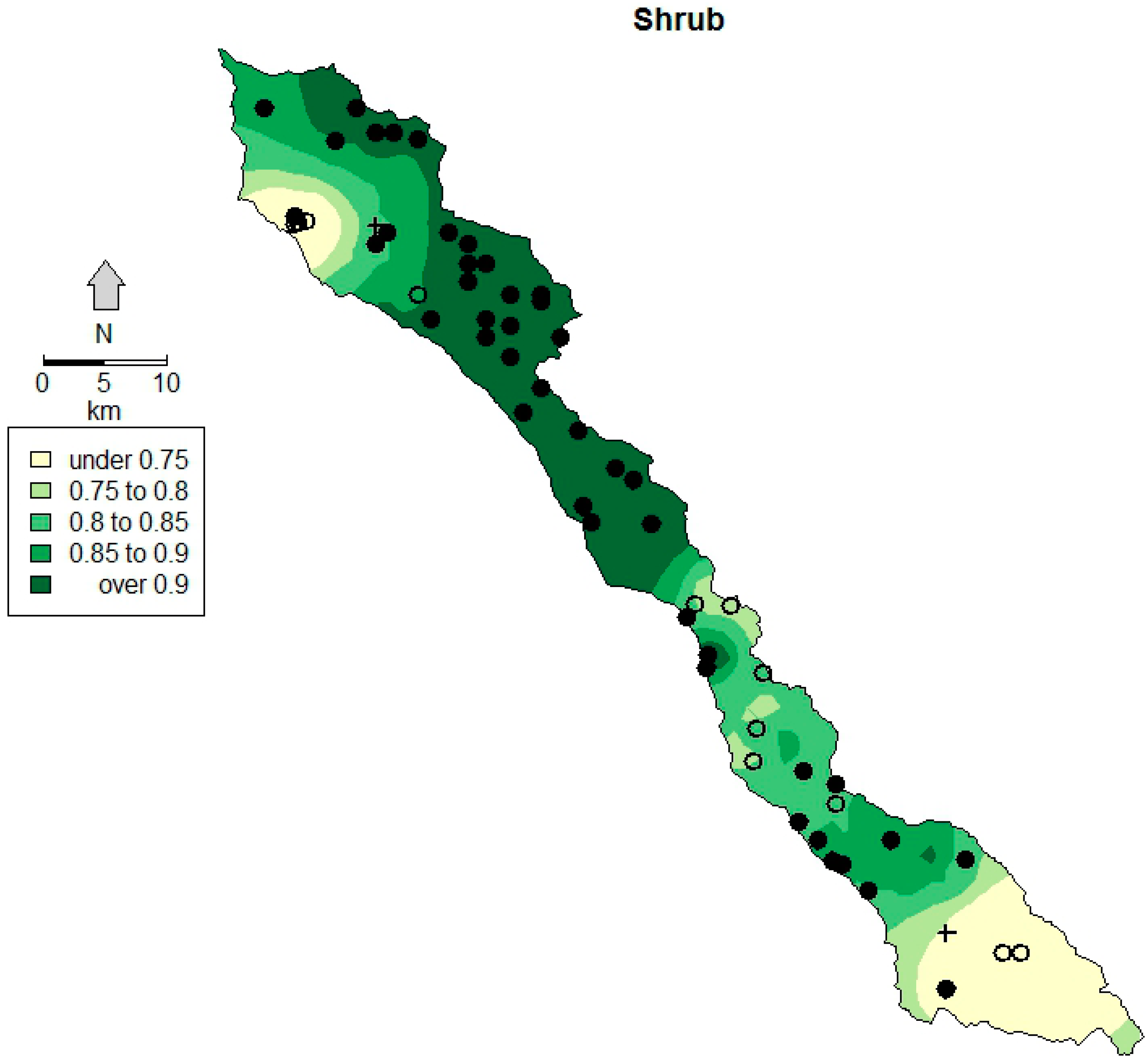
57]. The global measure of the 2012 overall classification accuracies was high; however, the shrub cover class contained relatively high errors of both commission and omission. Figure 4 illustrates spatial patterns of predicted accuracy, including a lower probability of accuracy in the northern and southern portions of the study area and a higher probability of accuracy in the central portion. For both portions, but especially in the south, a lack of training data likely hindered accuracy. The southern area also reflects the driest portion of the study and a transition to a greater proportion of more drought-tolerant shrub species [9]. The northern site, by contrast, is a site where the coastal marine layer pools and intrudes inland, as is visible on the numerous Landsat scenes we reviewed, and this may increase vegetation vigor (altering the spectral signal) and induce misclassification. This type of spatially explicit accuracy is useful, as it can inform the appropriate choice of land cover data for an application [58] or where specific portions or regions of a land cover map are not appropriate to be used for subsequent analysis or land management planning [57]. For large, difficult-to-access study sites, this can indicate local problem areas in the classification method and highlight regions of the study area where additional data are needed [59].
The base 2012 year classification exhibited high accuracy; however, the accuracy was not as high for the preceding years. While it is possible that this reduced accuracy is partially attributed to either overfitting the tree to the 2012 field data, this is unlikely given the simplicity of the tree that we utilized. There is greater potential that inaccuracy in the earlier years stems from spectral differences resulting from interannual variability in vegetation phenology and soil moisture. Though phenology is relatively static during the months of remotely sensed data acquisition for this region (i.e., vegetation is mostly dormant by early July), interannual climate variability can easily produce differences in vegetation vigor and cover between years. For example, the study area received only 50 percent of normal precipitation in 2007 (based on a 30-year climatological average) [60], and the drought stress likely reduced the vigor of the shrubs, making shrubland reflectance more similar to a forest spectral signature. Similarly, the timing of moisture can affect grass classification accuracies, as late spring precipitation or even strong marine layers (which occur in the summer on the central California coast when there is high pressure in California’s Central Valley) can induce temporary green-up in annual grasses, leading to misclassification as shrubs.
It is also unsurprising that the accuracies were lower for the years prior to 2012, because we excluded the portion of the study area with the highest classification accuracy (the burned areas) from the accuracy assessment. We were using primarily persistent sites to validate prior to 2012, and the area within the wildfire perimeters was considered disturbed (and not persistent). Therefore, while the classification accuracy for 2012 included field data collected in the fire perimeters for the validation, the accuracies for the prior years did not include validation within the burned areas, and our spatial GWR of accuracy indicated that the highest accuracy occurred in the burned areas in 2012.
Though the classifications of seven historic Landsat scenes were less accurate compared to the 2012 base classification, overall, the classification produced land cover maps of moderate to high accuracy, and we assume that the true accuracy is actually higher based on our exclusion of validation sites from the burned areas due to the lack of persistence. We are confident that using these land cover maps will be sufficient in determining the effects of the 2008 wildfire on land cover and to the nearshore ecosystem.

5. Conclusions

Transitions in land cover and the disturbances that drive these transitions play a vital role in the function of ecosystems. Quantifying these changes relies on their inclusion into land cover datasets. Ample amounts of remotely sensed data provide many opportunities for the classification of land cover for monitoring land cover changes; however, a lack of field data can make it difficult to use many classification methods. We present a simple method for classifying historic remotely sensed data in the absence of historic reference data given at least one year of quality reference data is available. Using this method, we successfully classified eight years of Landsat data with relative accuracy, including years that incorporated the impacts of wildfire. While this study is by no means exhaustive, it points to an alternative approach to the current practice of using whatever the most recently available land cover data set is for ecological studies, even when there are known changes in land cover likely to affect the analysis and study findings.

Acknowledgments

The research was supported by NSF Idaho EPSCoR under Award Number EPS-0814387, NASA Award NNX10AT77A and the USGS Global Climate Change Office through the Pacific Nearshore Project. The authors thank Jeff Hicke and Phil Higuera for insights that substantially improved the manuscript.

Author Contributions

Katherine D. Morrison collected data, designed and conducted the data analysis, interpreted results and prepared the manuscript. Crystal A. Kolden assisted with research design, result interpretation and contributed to manuscript preparation and revision.

Conflicts of Interest

The authors declare no conflict of interest.

References

  1. Lambin, E.F.; Turner, B.L.; Geist, H.J.; Agbola, S.B.; Angelsen, A.; Bruce, J.W.; Coomes, O.T.; Dirzo, R.; Fischer, G.; Folke, C.; et al. The causes of land-use and land-cover change: Moving beyond the myths. Glob. Environ. Chang. 2001, 11, 261–269. [Google Scholar]
  2. Turner, M. Landscape ecology: The effect of pattern on process. Annu. Rev. Ecol. Syst. 1989, 20, 171–197. [Google Scholar]
  3. Turner, M.; Dale, V. Comparing large, infrequent disturbances: What have we learned? Ecosystems 1998, 1, 493–496. [Google Scholar]
  4. Dale, V.H.; Joyce, L.A.; Mcnulty, S.; Neilson, R.P.; Ayres, M.P.; Flannigan, M.D.; Hanson, P.J.; Irland, L.C.; Lugo, A.E.; Peterson, C.J.; et al. Climate change and forest disturbances. Bioscience 2001, 51, 723–734. [Google Scholar]
  5. Epting, J.; Verbyla, D.; Sorbel, B. Evaluation of remotely sensed indices for assessing burn severity in Interior Alaska using Landsat TM and ETM+. Remote Sens. Environ. 2005, 96, 328–339. [Google Scholar]
  6. Patterson, M.; Yool, S. Mapping fire-induced vegetation mortality using Landsat Thematic Mapper data: A comparison of linear transformation techniques. Remote Sens. Environ. 1998, 65, 132–142. [Google Scholar]
  7. Robichaud, P.; Beyers, J.; Neary, D. Evaluating the Effectiveness of Postfire Rehabilitation Treatments; U.S. Department of Agriculture: Washington, DC, USA, 2000; p. 89. [Google Scholar]
  8. Sleeter, B.M.; Wilson, T.S.; Soulard, C.E.; Liu, J. Estimation of late Twentieth Century land-cover change in California. Environ. Monit. Assess. 2011, 173, 251–266. [Google Scholar]
  9. Davis, F.W.; Borchert, M.I. Central coast bioregion. In Fire in Califorina’s Ecosystems; Sugihara, N.G., Wagtendonk, J.W., Shaffer, K.E., Fites-Kaufman, J., Thode, A.E., Eds.; University of California Press: Oakland, CA, USA, 2006; p. 596. [Google Scholar]
  10. Goodridge, B.M.; Melack, J.M. Land use control of stream nitrate concentrations in mountainous coastal California watersheds. J. Geophys. Res. Biogeosci. 2012, 117, 1–17. [Google Scholar]
  11. Bowen, L.; Miles, A.; Kolden, C.; Saarinen, J.; Murray, M.; Tinker, T. Effects of wildfire on sea otter (Enhydra lutris) immune function. Mar. Mammal Sci. 2014. [Google Scholar] [CrossRef]
  12. Venn-Watson, S.; Smith, C.R.; Jensen, E.D.; Rowles, T. Assessing the potential health impacts of the 2003 and 2007 firestorms on bottlenose dolphins (Trusiops trucatus) in San Diego. Inhal. Toxicol. 2013, 29, 481–491. [Google Scholar]
  13. U.S. Fish & Wildlife Service Species Profile: Southern Sea Otter. Available online: http://ecos.fws.gov/speciesProfile/profile/speciesProfile.action?spcode=A0A7 (accessed on 11 March 2014).
  14. Bodkin, J.; Ballachey, B.; Dean, T.; Fukuyama, A.; Jewett, S.; McDonald, L.; Monson, D.; O’Clari, C.; VanBlaricom, G. Sea otter population status and the process of recovery from the 1989 “Exxon Valdez”oil spill. Mar. Ecol. Prog. Ser. 2002, 241, 237–253. [Google Scholar]
  15. Johnson, C.K.; Tinker, M.T.; Estes, J.A.; Conrad, P.A.; Staedler, M.; Miller, M.A.; Jessup, D.A.; Mazet, J.A.K. Prey choice and habitat use drive sea otter pathogen exposure in a resource-limited coastal system. Proc. Natl. Acad. Sci. USA 2009, 106, 2242–2247. [Google Scholar]
  16. Conrad, P.A.; Miller, M.A.; Kreuder, C.; James, E.R.; Mazet, J.; Dabritz, H.; Jessup, D.A.; Gulland, F.; Grigg, M.E. Transmission of Toxoplasma: Clues from the study of sea otters as sentinels of Toxoplasma gondii flow into the marine environment. Int. J. Parasitol. 2005, 35, 1155–1168. [Google Scholar]
  17. Miller, M.A.; Kudela, R.M.; Mekebri, A.; Crane, D.; Oates, S.C.; Tinker, M.T.; Staedler, M.; Miller, W.A.; Toy-Choutka, S.; Dominik, C.; et al. Evidence for a novel marine harmful algal bloom: Cyanotoxin (microcystin) transfer from land to sea otters. PLoS One 2010, 5. [Google Scholar] [CrossRef]
  18. Kolden, C.A.; Abatzoglou, J.T. wildfire consumption and interannual impacts by land cover in Alaskan boreal forest. Fire Ecol. 2012, 7, 98–114. [Google Scholar]
  19. Eidenshink, J.; Schwind, B.; Brewer, K.; Zhu, Z.; Quayle, B.; Howard, S.; Falls, S. A project for monitoring trends in burn severity. Fire Ecol. 2007, 3, 3–21. [Google Scholar]
  20. Brewer, C.K.; Winne, J.C.; Redmond, R.L.; Opitz, D.W.; Mangrich, M.V. Classifying and mapping wildfire severity: A comparison of methods. Photogramm. Eng. Remote Sens. 2005, 71, 1311–1320. [Google Scholar]
  21. Clark, J.; Parsons, A.; Zajkowski, T.; Lannom, K. Remote Sensing Imagery Support for Burned Area Emergency Response Teams on 2003 Southern California Wildfires; Remote Sensing Applications Center: Salt Lake City, UT, USA, 2003; p. 22. [Google Scholar]
  22. Kennedy, R.E.; Yang, Z.; Cohen, W.B. Detecting trends in forest disturbance and recovery using yearly Landsat time series: 1. LandTrendr—Temporal segmentation algorithms. Remote Sens. Environ. 2010, 114, 2897–2910. [Google Scholar]
  23. Cohen, W.B.; Yang, Z.; Kennedy, R. Detecting trends in forest disturbance and recovery using yearly Landsat time series: 2. TimeSync—Tools for calibration and validation. Remote Sens. Environ. 2010, 114, 2911–2924. [Google Scholar]
  24. Lu, D.; Weng, Q. A survey of image classification methods and techniques for improving classification performance. Int. J. Remote Sens. 2007, 28, 823–870. [Google Scholar]
  25. Breiman, L.; Freedman, J.; Olshen, R.; Stone, C. Classification and Regression Trees; Wadsworth: Belmont, CA, USA, 1984. [Google Scholar]
  26. Friedl, M.; Brodley, C. Decision tree classification of land cover from remotely sensed data. Remote Sens. Environ. 1997, 61, 399–409. [Google Scholar]
  27. Zambon, M.; Lawrence, R.; Bunn, A.; Powell, S. Effect of alternative splitting rules on image processing using classification tree analysis. Photogramm. Eng. Remote Sens. 2006, 72, 25–30. [Google Scholar]
  28. Rogan, J.; Miller, J.; Stow, D.; Franklin, J. Land-cover change monitoring with classification trees using Landsat TM and ancillary data. Photogramm. Eng. Remote Sens. 2003, 69, 793–804. [Google Scholar]
  29. Hubert-Moy, L.; Cotonnec, A.; Le Du, L. A comparison of parametric classification procedures of remotely sensed data applied on different landscape units. Remote Sens. Environ. 2001, 75, 174–187. [Google Scholar]
  30. Hansen, M.C.; DeFries, R.S.; Townshend, J.R.; Sohlberg, R. Global land cover classification at 1 km spatial resolution using a classification tree approach. Int. J. Remote Sens. 2000, 21, 1331–1364. [Google Scholar]
  31. Yang, X.; Lo, C.P. Using a time series of satellite imagery to detect land use and land cover changes in the Atlanta, Georgia metropolitan area. Int. J. Remote Sens. 2002, 23, 1775–1798. [Google Scholar]
  32. Lentile, L.B.; Holden, Z.A.; Smith, A.M.S.; Falkowski, M.J.; Morgan, P.; Lewis, S.A.; Gessler, P.E.; Benson, N.C. Remote sensing techniques to assess active fire characteristics and post-fire effects. Int. J. Wildland Fire 2006, 15, 319–345. [Google Scholar]
  33. Homer, C.; Huang, C.; Yang, L.; Wylie, B.; Coan, M. Development of a 2001 National Landcover Database for the United States. Photogramm. Eng. Remote Sens. 2004, 70, 829–840. [Google Scholar]
  34. Morrison, K.M.; Kolden, C.A. Impacts of wildfire on coastal watersheds and the nearshore environment in Big Sur, California. J. Env. Manag. 2014. under review. [Google Scholar]
  35. Davis, F.W.; Borchert, M.; Meentemeyer, R.K.; Flint, A.; Rizzo, D.M. Pre-impact forest composition and ongoing tree mortality associated with sudden oak death in the Big Sur region; California. For. Ecol. Manag. 2010, 259, 2342–2354. [Google Scholar]
  36. Myers, N.; Mittermeier, R.A.; Mittermeier, C.G.; da Fonseca, G.A.; Kent, J. Biodiversity hotspots for conservation priorities. Nature 2000, 403, 853–858. [Google Scholar]
  37. Masek, J.; Vermote, E. A Landsat surface reflectance dataset for North America, 1990–2000. IEEE Geosci. Remote Sens. Lett. 2006, 3, 68–72. [Google Scholar]
  38. Chander, G.; Markham, B.L.; Helder, D.L. Summary of current radiometric calibration coefficients for Landsat MSS, TM, ETM+, and EO-1 ALI sensors. Remote Sens. Environ. 2009, 113, 893–903. [Google Scholar]
  39. Tucker, C.J. Red and photographic infrared linear combinations for monitoring vegetation. Remote Sens. Environ. 1979, 8, 127–150. [Google Scholar]
  40. Rouse, J.W.; Haas, J.A.; Schell, J.A.; Deering, D.W.; Harlan, J.C. Monitoring the Vernal Advancement of Retrogradation of Natural Vegetation; NASA Goddard Space Flight Center: Greenbelt, MD, USA, 1974; p. 371. [Google Scholar]
  41. Key, C.H.; Benson, N.C. Landscape Assessment (LA) Sampling and Analysis Methods; USDA Forest Service Gen. Technical Report RMRS-GTR-164-CD; U.S. Department of Agriculture: Washington, DC, USA, 2006; p. 55. [Google Scholar]
  42. Jensen, J.R. Biophysical remote sensing. Ann. Assoc. Am. Geogr. 1983, 73, 111–132. [Google Scholar]
  43. Jensen, J.R. Remote Sensing of the Environment An Earth Resource Perspective, 2nd ed.; Pearson Prentice Hall: Upper Saddle River, NJ, USA, 2007; p. 592. [Google Scholar]
  44. Smith, A.M.S.; Wooster, M.J.; Drake, N.A.; Dipotso, F.M.; Falkowski, M.J.; Hudak, A.T. Testing the potential of multi-spectral remote sensing for retrospectively estimating fire severity in African Savannahs. Remote Sens. Environ. 2005, 97, 92–115. [Google Scholar]
  45. Crist, E.P. A TM tasseled cap equivalent transformation for reflectance factor data. Remote Sens. Environ. 1985, 306, 301–306. [Google Scholar]
  46. Ghimire, B.; Rogan, J.; Miller, J. Contextual land-cover classification: Incorporating spatial dependence in land-cover classification models using random forests and the Getis statistic. Remote Sens. Lett. 2010, 1, 45–54. [Google Scholar]
  47. Atkinson, P.; Lewis, P. Geostatistical classification for remote sensing: An introduction. Comput. Geosci. 2000, 26, 361–371. [Google Scholar]
  48. Wulder, M.; Boots, B. Local spatial autocorrelation characteristics of remotely sensed imagery assessed with the Getis statistic. Int. J. Remote Sens. 1998, 19, 2223–2231. [Google Scholar]
  49. Jensen, J.R. Introductory Digital Image Processing, 3rd ed.; Prentice Hall: Upper Saddle River, NJ, USA, 2005; p. 526. [Google Scholar]
  50. Franklin, J.; McCullough, P.; Gray, C. Terrain variables used for predictive mapping of vegetation communities in southern California. In Terrain Analysis: Principles and Applications; Wilson, J.P., Gallant, J.C., Eds.; John Wiley & Sons, Inc.: Hoboken, NJ, USA, 2000; pp. 331–353. [Google Scholar]
  51. Pal, M.; Mather, P.M. An assessment of the effectiveness of decision tree methods for land cover classification. Remote Sens. Envron. 2003, 86, 554–565. [Google Scholar]
  52. Congalton, R.G.R. A review of assessing the accuracy of classifications of remotely sensed data. Remote Sens. Environ. 1991, 37, 35–46. [Google Scholar]
  53. Comber, A.; Fisher, P.; Brunsdon, C.; Khmag, A. Spatial analysis of remote sensing image classification accuracy. Remote Sens. Environ. 2012, 127, 237–246. [Google Scholar]
  54. Fotheringham, S.A.; Brundsdon, C.; Charlton, M. Quantitative Geography; SAGE: London, UK, 2000; p. 270. [Google Scholar]
  55. Greenlee, J.; Langenheim, J. Historic fire regimes and their relation to vegetation patterns in the Monterey Bay area of California. Am. Midl. Nat. 1990, 124, 239–253. [Google Scholar]
  56. Wulder, M.; Franklin, S.; White, J.; Linke, J.; Magnussen, S. An accuracy assessment framework for large-area land cover classification products derived from medium-resolution satellite data. Int. J. Remote Sens. 2006, 27, 663–683. [Google Scholar]
  57. Foody, G.M. Local characterization of thematic classification accuracy through spatially constrained confusion matrices. Int. J. Remote Sens. 2005, 26, 1217–1228. [Google Scholar]
  58. Comber, A. Geographically weighted methods for estimating local surfaces of overall, user and producer accuracies. Remote Sens. Lett. 2013, 4, 373–380. [Google Scholar]
  59. Kyriakidis, P.; Dungan, J. A geostatistical approach for mapping thematic classification accuracy and evaluating the impact of inaccurate spatial data on ecological model predictions. Environ. Ecol. Stat. 2001, 8, 311–330. [Google Scholar]
  60. California Department of Water Resources (CDWR). California’s Drought of 2007–2009: An Overview; CDWR: Sacramento, CA, USA, 2010; p. 128. [Google Scholar]

