Integrating Forest Cover Change with Census Data: Drivers and Contexts from Bolivia and the Lao PDR

Abstract

The aim of this paper is to explore possible links between forest cover change and characteristics of social-ecological systems at sub-national scale based mainly on census data. We assessed relationships between population density, poverty, ethnicity, accessibility and forest cover change during the last decade for four regions of Bolivia and the Lao PDR, combining a parcel-based with a cell-based approach. We found that accessibility is a key driver of forest cover change, yet it has the effect of intensifying other economic and policy-related underlying drivers, like colonization policies, cash crop demand, but also policies that lead to forest gain in one case. Poverty does not appear as a driver of deforestation, but the co-occurrence of poverty and forest loss driven by external investments appears critical in terms of social-ecological development. Ethnicity was found to be a moderate explanatory of forest cover change, but appears as a cluster of converging socio-economic characteristics related with settlement history and land resource access. The identification of such clusters can help ordering communities into a typology of social-ecological systems, and discussing their possible outcomes in light of a critical view on forest transition theory, as well as the relevance and predictive power of the variables assessed.

1. Introduction

The integration of remotely sensed data on land cover with data related with decisions of land managers has been identified as a key challenge of land change science [1]. However, theory and practice related with land use and land cover change (LULC) as well as with natural resources governance have long evolved in parallel. In both cases, they have sought to overcome traditional oversimplifications and built new approaches to address the complexity of human-environment relationships at multiple scales.

Several challenges have been identified as being inherent to the integration of social, natural and geographical information sciences: the aggregation and inference of data, the link between land users and remotely sensed information, data quality and validation, spatial-temporal mismatch, use of ancillary information, spatial autocorrelation and accuracy assessment [1]. On the other hand, governance theory has developed a social-ecological framework, which seeks to address multiple levels of variables ordered in a way that enables diagnosing social-ecological systems (SES) and look for patterns across large numbers of cases [2]. The framework faces however the challenge of the cost and difficulty of assessing key variables beyond the local scale for large samples.

This paper has the objective of exploring possible links between land cover change and characteristics of social-ecological systems that can be derived from data available for a relatively large number of cases in a defined region. We focus on the relationships between forest cover change and some characteristics of social-ecological systems, namely poverty, ethnicity and accessibility in four sub-national regions of two developing countries, the Plurinational State of Bolivia (further: Bolivia) and the Lao People’s Democratic Republic (Further: Laos). In these countries, a relatively good corpus of case studies and national scale data exist, but there are relatively little data at intermediary scales. At broader scales, census data represent the main source of socio-economic information and only a few land cover datasets are available. Considering this limitation, we explore what kind of relationships can reasonably be made visible at sub-national scale using census data, simple land cover assessments and simple statistics. Contrary to most studies on land change that are based on cell-based spatial units only (i.e., pixels), we chose a combination of analysis based on (1) hexagonal cells and (2) local communities as main observation units using a village polygon-based approach developed by Messerli et al. [3]. We discuss then the obtained results in light of existing case studies within the regions chosen.

1.1. Forest Cover Change and Social-Ecological Systems: Overcoming Simplifications

Land change science has been defined by Turner et al. as the “interdisciplinary field [that] seeks to understand the dynamics of land cover and land use as a coupled human-environment system” [4] (p. 20666). According to these authors, it includes four main fields of research: (1) the observation and monitoring of land changes; (2) the proper understanding of these changes as a coupled human–environment system; (3) the modeling of land change and (4) the assessment of system outcomes. In this study, we focus specifically on the understanding of land cover change as a coupled human–environment system.

In the past, the causes of land use and land cover change (LULC) have often been misinterpreted and oversimplified in relation with a single factor, like population, poverty, technology or socio-economic inequalities [5]. It is now widely acknowledged that the causes of LULC are complex and result from the interaction between social, political, economic, demographic, technological, cultural and biophysical variables [6]. According to Lambin et al. [7], identifying the causes of land changes requires an understanding of how people make land-use decisions, and distinguish between proximate causes, which are the direct human actions that operate at the local level and physically affect land cover, and underlying causes, which rely on a more complex array of social, political, economic, demographic, technological, cultural and biophysical variables. Underlying causes alter proximate causes; they often originate at higher levels of organizations, from regional to global, and local communities have little control over them [7,8].

Deforestation has been defined as the conversion of forest to another land cover type, or the fall of tree canopy below a defined threshold [7]. In their meta-analysis of 152 case studies within the tropics, Geist and Lambin [6] have identified infrastructure extension, agricultural expansion and wood extraction, but also biophysical factors like drought induced forest fires in the Amazon basin, as the main proximate causes of deforestation. Economic/technological, demographic, institutional and cultural factors are identified as underlying causes of forest conversion. Economic factors embrace the general expansion of cash economy and expanding markets, and agrotechnological changes that were observed to tend to encourage more deforestation [6]. Institutional factors include incentives for land based activities, infrastructure expansion (especially roads), and also legalization of land titles. Demographic factors are usually linked with in-migration and colonization, but rarely with fertility rates. Cultural factors have been shown to underlie economic and political forces, as for example in the cultural preference for cattle ranching found in some regions of Latin America [9]. An important finding of this overall meta-analysis is that the identified factors usually do not operate alone. In most cases, multiple causal factors and their interaction have led to deforestation.

The challenge of overcoming traditional simplifications and addressing multiple causal factors is also faced by the further development of natural resources governance theory. Natural resources governance is defined as “the broader arena in which institutions operate and the various management-related concepts take place” [10] (p. 491). In this body of knowledge, traditional simplifications have included “panaceas”, which “predict optimal performance if specific institutional arrangements are in place” [2] (p. 451). Nowadays, it is widely acknowledged that social-ecological systems are characterized by multivariable, non-linear and cross-scale processes [11]. Ostrom et al. [2] have developed a diagnostic approach for the analysis of social-ecological systems based on a series of variables meant to be unpacked until the analyst has found the disturbance that may affect a SES. These authors set up an agenda for future work that includes the accumulation of empirical data on social and ecological variables at multiple levels of aggregation. They require the performance of a large number of case studies, their meta-analysis and the search for patterns across cases using descriptive and inferential statistics. As they state [2] (p. 460), comparisons should allow building typological theories, that “specify independent variables, delineates them into the categories to be measured, and provide hypotheses and generalizations” [12]. Can land change science already perform contributions to the research agenda of elaborating typologies of social-ecological systems? Without replacing the need for in-depth field studies, we argue that using land cover change data in combination with census data can help to identify different types of social-ecological contexts and give useful orientations for both research and policy making.

1.2. Key Variables and Hypotheses

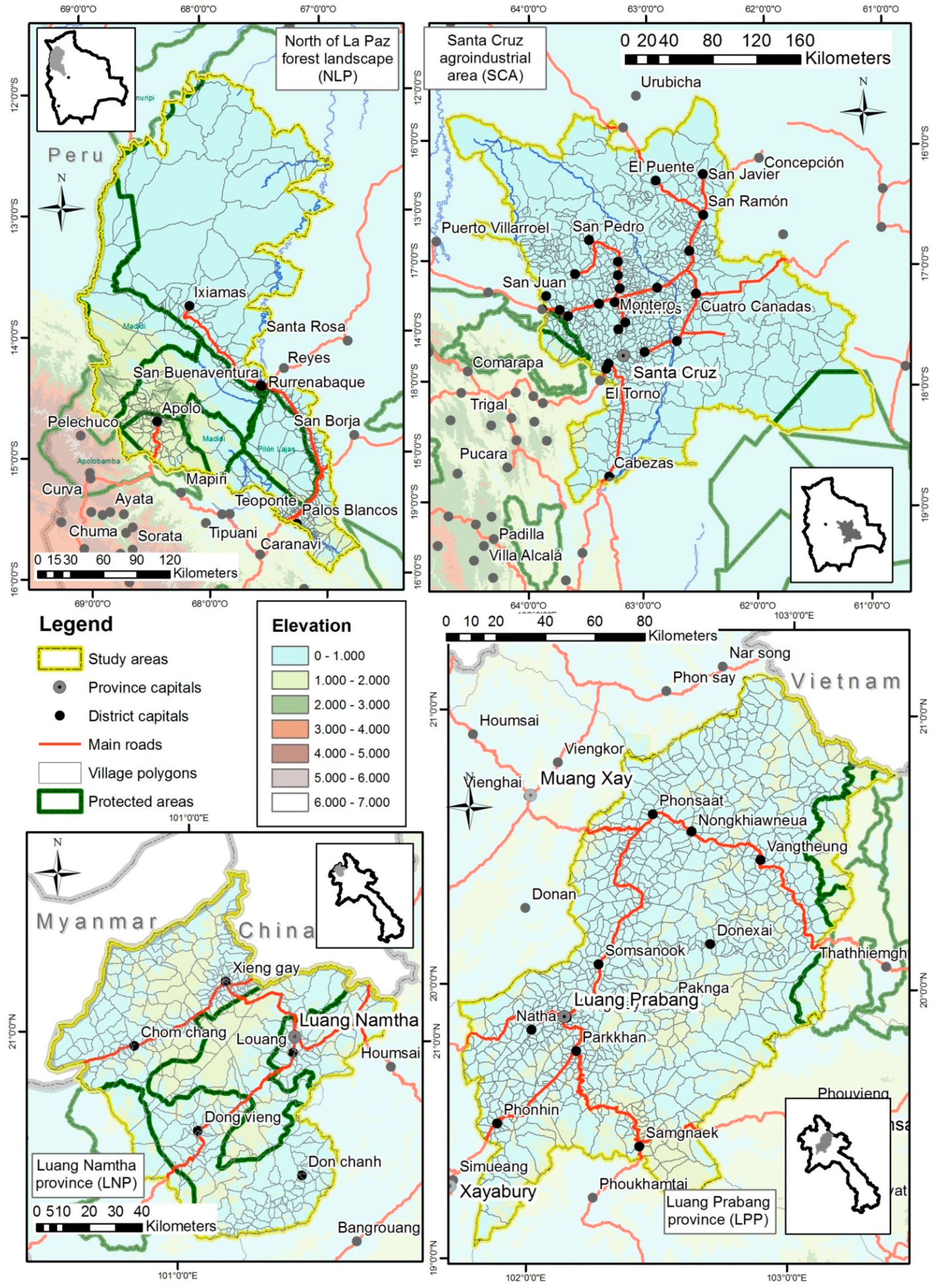
Our review on drivers of forest cover change allows the consideration of some key variables with more details. The relation between population and forest cover change is often linked to policy-driven or spontaneous rural migration [13]. Accessibility, understood in terms of travel time to urban centers, markets and roads, plays a key role [6,14].

The Forest Transition Theory links forest cover change with more general development aspects. The theory is based on the observation that in many now developed countries, initial population growth led to deforestation, but then industrialization and urbanization led to a shift from net forest loss to net forest gain, due to the concentration of agricultural production in smaller areas of better land [15]. Recent studies in Latin America [16] and Asia [17] support this view. Poverty is an important aspect of development and has often been associated with environmental degradation, poor people being deemed too poor to invest in natural resource management and trapped into a downward spiral of population growth, resource degradation and further impoverishment [18]. According to this view, poverty reduction would alleviate pressure on natural resources and be beneficial to the environment. A classical model to understand the relations between development and environment is the Environmental Kuznets Curve [19], which predicts an initial increase of environmental degradation with development followed by a decrease linked with an economic transition to services. The Forest Transition Theory is considered an application of the Environmental Kuznets Curve [20], with global studies showing that, for example, deforestation has stopped in countries with a per capita GDP exceeding $6400 [21].

Several scholars have pointed out the shortcomings of both Environmental Kuznets and Forest Transition models. First, from the point of view of involved people, deforestation is an investment in economically more interesting land uses [22]. This implies that poor people without access to technology assets are likely to have a limited impact on deforestation, but also that with development, they become able to clear more forest, as observed in many Latin American countries [22]. At that stage, the pathway to forest transition is still a long process, and irreversible biodiversity losses might occur before it is reached [23]. Another argument is that wealthy nations tend to export their most polluting activities to poorer nations [24], and consumption habits and fossil fuel dependence continuously increase with growing wealth [23]. Third, political ecologists have shown how development of industrial activities may further impoverish the most vulnerable populations by degrading the resources they rely on [25]. Finally, the Forest Transition Theory does not make a difference between natural forests and plantations, which are very different ecologically. The expansion of industrial tree plantations, erroneously linked to forest transition, suppose a further exploitation of natural resources, decline in biodiversity and emergence of environmental conflicts [26].

Investigating the relationship between poverty and forest cover change at disaggregated levels can make interesting contributions to this debate by addressing the heterogeneity of forest cover change within different socio-economic contexts. Rural poverty is often linked with remoteness and overlaps with the presence of natural forests [23], but also with the presence of socially and economically disadvantaged groups, often belonging to ethnic minorities as it has been shown in the case of Vietnam [27]. On the other hand, ethnicity is also often associated with specific natural resource—including land and forests—management patterns [28,29].

Assuming that forest transition occurs gradually in time and space within an area, we can formulate a first hypothesis that forest loss occurs mainly in agricultural frontier areas characterized by intermediate poverty and remoteness, while more developed, densely populated and largely deforested areas now experience forest increase. Most remote and poorest areas would tend to experience no change forest increase due to low population density and out-migration. The second hypothesis is that forest transitions differ among regional socio-economic contexts: the mentioned pattern is likely to be more visible in areas linked to international markets than areas oriented at subsistence and local markets. Considering ethnic groups leads us to formulate a third hypothesis: ethnicity might capture specific natural resource management and development contexts. They might form observable clusters with shared characteristics of remoteness, poverty and forest cover change, which can be used to identify types of social-ecological contexts.

1.3. Area of Study

Bolivia and the Lao PDR were chosen because they share some characteristics. While at the same time inserted in very different continental contexts, both countries are landlocked developing countries without fluvial ports to the sea, thus facing important barriers to their economic integration [30,31]. As a matter of fact, both Bolivia and the Lao PDR have among the lowest Gross Domestic Product (GDP) and development level in their respective regions. However, they also have lower population densities than their neighbors, highly uneven distributed populations, high ethnic diversity with 45 languages spoken in Bolivia and 84 in Laos [32], and the highest per capita forest cover in their respective regions. In this sense, Bolivia and the Lao PDR can be considered countries with low economic but high natural capital in the sense of Costanza et al. [33].

Both countries are also undergoing rapid changes including sustained economic growth and increased integration with their BRIC neighbors, Brazil and China, respectively, which enhances infrastructure development and cash crop expansion. Between 2000 and 2010, both countries were losing about 0.5% of their forest cover per year, which approximatively corresponds to the regional average (0.4% of yearly loss for Southeast Asia and 0.5% for South America) [34]. Nevertheless, Bolivia has been mentioned as one of the current emerging deforestation hotspots [35]. On the other hand, both countries have recently enacted several reforms on environment, land, and forest governing policies. These also include decentralization reforms which recognized local communities as legal entities and partly handed over natural resources governance to them, making these communities pertinent as units of observation.

In Bolivia, land redistribution and economic development policies have had a strong influence on forest conversion to cropland in the Eastern lowlands, where roads were opened and land was distributed to Andean and foreign colonists since the 1960s [36,37]. Since 1996, a process of land title regularization was launched, which recognizes indigenous territories (called Tierras Comunitarias de Origen, TCO), small properties, as well as medium and large landholdings. During the 1990s, large forested lowlands were also declared protected. In 2006, the “Law of agrarian reform renewal” was enacted by pro-indigenous and pro-peasant President Evo Morales. After that enactment, the title regularization process was emancipated from international cooperation, led by the State, and accelerated [38]. However, the law also instituted the clause of “socio-economic function of land” that foresees the verification of economic activities in large landholdings, and their expropriation by the State in case of it could not be established [39]. Because socio-economic function is often displayed by the physical measure of forest clearing on the parcel, the law acts as an institutional incentive for deforestation [40].

In Bolivia, Andean native ethnic groups (mainly Quechua and Aymara) make up about 60% of total population [41]. Since the 1960s, the Bolivian government has been promoting successive programs of land distribution and colonization of the formerly sparsely populated lowlands to Andean colonists as well as to foreign settlers [36,37]. Nowadays, the Bolivian lowlands are characterized by a high diversity of economic rural actors that are also partly linked to ethnic groups. Mestizo and foreign settlers practice medium to large scale mechanized cultivation or extensive cattle ranching. Andean settlers (most of indigenous Quechua and Aymara origin) are small to medium producers with no or little mechanization, oriented toward the national market, typically owning between 10 and 20 ha of land and leaving part of it fallow. Lowland indigenous peoples, distributed into more than 30 different groups, make up less than 10% of the total Bolivian population. They are mainly subsistence farmers practicing shifting cultivation and the collection of Non-Timber Forest Products (NTFP) [36]. Since the 1990s, onto the 2000s, they have also been granted large, though highly fragmented indigenous territories (Tierras Comunitarias de Origen TCO) [42].

The two lowland regions chosen in this study represent different combinations of economic and ethnic diversity (Figure 1; Table 1). The North of La Paz forest landscape (NLP) is mainly inhabited by lowland indigenous peoples as well as by Andean colonists who concentrate their settlements along roads opened mainly during the 1980s. The area is part of the “Tambopata-Madidi greater landscape” and includes a network of protected areas and indigenous territories aimed at conserving one of the most biologically diverse areas in the world, shared between Bolivia and Peru. The Santa Cruz agroindustrial area (SCA), also called “Santa Cruz integrated North” has been at the same time a pole of national economic development and deforestation since the 1970s [43] and made up 60% of total deforestation in Bolivia until 1994 [44]. Highly mechanized cultivation aimed at export markets, especially soybeans, have been constantly expanding around the city of Santa Cruz, encroaching into forested areas and co-existing with areas of Andean colonization along the roads to the cities of Cochabamba and Trinidad.

Figure 1. Overview of the four study areas.

Figure 1. Overview of the four study areas.

Table 1. Main characteristics of the study areas.

	North La Paz	Santa Cruz	Luang Prabang	Luang Namtha
Area (km2)	49,304	68,520	20,009	9533
Number of villages/communities	259	626	765	341
Total population	82,721	1,625,735	425,354	159,119
Population excluding urban areas	59,556	340,305	334,221	122,767
Population density (h/km2)	1.7	23.8	21.3	16.7
Poverty (%)	89.3	37.3	40.1	36.2
Extreme poverty (%)	45.7	14.7
Total forest cover t0 *, (km2)	38,752	40,006	7178	5668
Total forest cover t1 *, (km2)	38,709	32,076	9618	5518
Percent of forest cover, t0	78.6	58.4	35.9	59.5
Percent of forest cover, t1	78,5	46.8	48.0	57.9
Annual forest cover change rate (t0–t1)	−0.00012	−0.0246	0.0293	−0.0027
Ethnic categories (% of population)
Andean	47.6	22.0
Lowland indigenous	12.9	10.7
Non-native	39.5	67.3
Ethnic Lao (Tai-Kadai)			52.8	47.0
Austroasiatic			35.0	19.1
Hmong-Mien and Sino-Tibetan			12.2	33.9

* t₀ = 2001 in Bolivia; 2000 in Laos; t₁ = 2010 in both countries.

Table 1. Main characteristics of the study areas.

	North La Paz	Santa Cruz	Luang Prabang	Luang Namtha
Area (km2)	49,304	68,520	20,009	9533
Number of villages/communities	259	626	765	341
Total population	82,721	1,625,735	425,354	159,119
Population excluding urban areas	59,556	340,305	334,221	122,767
Population density (h/km2)	1.7	23.8	21.3	16.7
Poverty (%)	89.3	37.3	40.1	36.2
Extreme poverty (%)	45.7	14.7
Total forest cover t0 *, (km2)	38,752	40,006	7178	5668
Total forest cover t1 *, (km2)	38,709	32,076	9618	5518
Percent of forest cover, t0	78.6	58.4	35.9	59.5
Percent of forest cover, t1	78,5	46.8	48.0	57.9
Annual forest cover change rate (t0–t1)	−0.00012	−0.0246	0.0293	−0.0027
Ethnic categories (% of population)
Andean	47.6	22.0
Lowland indigenous	12.9	10.7
Non-native	39.5	67.3
Ethnic Lao (Tai-Kadai)			52.8	47.0
Austroasiatic			35.0	19.1
Hmong-Mien and Sino-Tibetan			12.2	33.9

* t₀ = 2001 in Bolivia; 2000 in Laos; t₁ = 2010 in both countries.

Since the foundation of the Lao PDR in 1975, all land in Laos formally belongs to the State, but after the transition to market economy since 1986, citizens have rights to market their land by selling or renting. Land reforms were then enacted with the objectives of increasing land tenure security and eliminating shifting cultivation, considered as being destructive to upland ecosystems [45,46]. From 1993 onwards, the Land Use Planning and Land Allocation (LUPLA) policy was implemented, including delineation of village boundaries, zoning of villages into different land use types, and allocation of cultivation plots to individual households [47]. Zoning plans had the effect to separate farmland from forest land, removed large areas of the villages from the shifting cultivation cycle, and reduced the agricultural land per capita [45,46]. On the other hand, a resettlement policy, already starting 1975 and officialized later, relocated most remote populations near roads and towns to “benefit from rural development policies” [48]. Finally, a network of National Protected Areas was created after 1993 as well [46]. According to Lestrelin [46], resettlement and land allocation policies had a much larger impact in the upland areas, for which they were mainly meant: lowland paddy fields were not affected by the allocation process. Finally, more recently, a large number of land concessions have been granted by the Lao government to foreign companies, aimed at developing cash crops [49].

Laos is an ethnically very diverse country, with about the half of the population belonging to the ethnic Lao, and the rest to 48 officially recognized minorities. Ethnic Lao occupy most lowland areas, have had a dominant position, and have often disregarded highland groups [50]. In their first years in power, the revolutionary government used a tripartite system classifying ethnic groups by altitude: Lao Loum (lowlanders), Lao Theung (midlanders) and Lao Suung (highlanders) [51]. Though no more officially used, this classification corresponds roughly to the main ethnolinguistic families of Laos: Lao Loum belong mainly to the Tai-Kadai language family, Lao Theung to the Austroasiatic family and Lao Suung to the Miao-Yao and Tibeto-Burman linguistic families [52]. Though agricultural practices vary considerably from one village to another among the same ethnic group [53], most middle-land and highland ethnic minorities practice shifting cultivation systems, while rural lowlanders practice permanent, irrigated cultivation [54].

Two Lao provinces with a large share of ethnic minority population were chosen to carry out the study. The province of Luang Prabang (LPP), topographically and ethnically highly diverse, was one of the first areas where the land allocation policy was implemented [47]. There, the majority of currently existing villages have been resettled and/or have gone through the land allocation procedure [55]. The province of Luang Namtha (LNP) has a high proportion of Tibeto-Burman and Austroasiatic minorities, and has witnessed a rapid expansion of cash crops [56], particularly rubber, along the road linking the province to the Chinese border [57].

In the four study areas, we excluded very remote (>24 h of travel from next village) as well as strictly protected areas form the analysis. This includes the Madidi and Amboro National Parks in Bolivia. In the two Lao study areas, neither very remote nor strictly protected areas occurred.

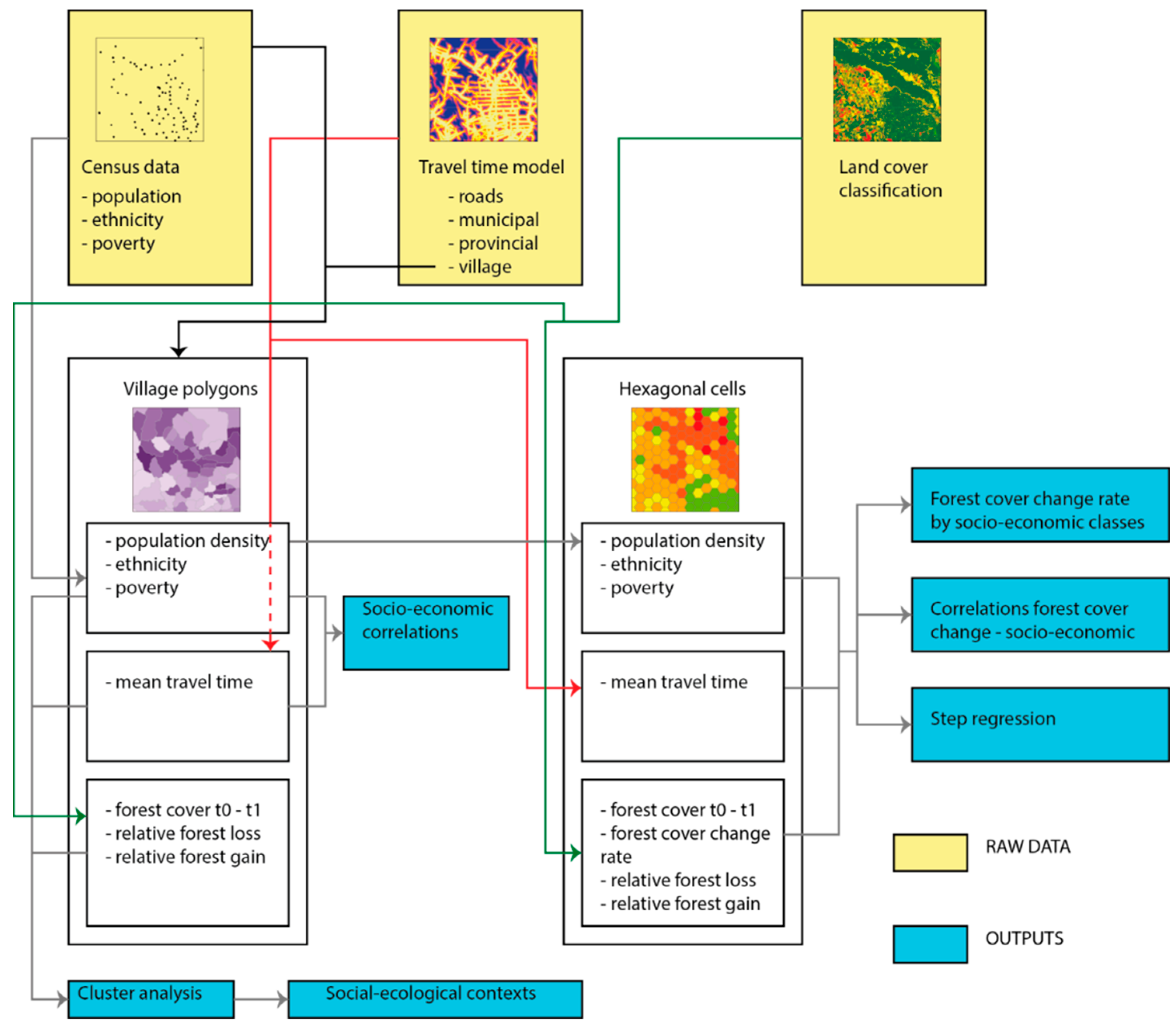
1.4. Approach and Methodology

Our approach is based on three datasets. Data on population, poverty and ethnicity were obtained from the Censo Nacional de Población y Vivienda 2001 (CNPV 2001) for Bolivia and the Population and Housing Census 2005 (PHC 2005) for Laos; data on accessibility is derived from cell-based travel cost models calculated in relation with roads, rivers, slope and land cover, and data on forest cover change was produced through supervised classification of Landsat-7 images.

1.4.1. Variables Derived from Census

In both countries, the lowest level of available census data is the village or locality level. In Laos, this corresponds to villages (Ban, $\stackrel{້}{ບ}$ານ). The Lao village represents an important land governance level, since its consolidation as a land management and policy implementation entity has been the target of LUPLA policies [47]. In Bolivia, localities with available census data were aggregated to communities, which group one up to about 20 localities in the CNPV 2001 database. In Bolivian rural areas, these communities usually correspond to legally recognized “basic territorial organizations” (Organizaciones Territoriales de Base OTB). OTBs are self-organized citizen groups (in rural areas often peasant unions and indigenous communities) which manage local natural resources, and mediate between individual citizens and municipal governments. Communities can be clustered villages but also dispersed settlements.

Ethnicity was assessed through the percentage of population belonging to three aggregated ethnic categories by village or community. Data on ethnic groups in Laos is based on main language, with indigenous languages widely spoken in the country. Data obtained from the PHC 2005, were aggregated as percentage of population of the village belonging to the main ethnolinguistic families present in the country: Tai-Kadai, Austroasiatic, Miao-Yao and Tibeto-Burman. The groups were then further aggregated to the traditional tripartite system used in Laos, with groups belonging to the Tai-Kadai family considered as majority ethnic Lao or Lao Loum; Austroasiatic groups as Lao Theung; and Miao-Yao and Tibeto-Burman merged in a single “highlander” category (Lao Suung) [52]. Ethnic group data in Bolivia is based on people’s (aged 15 and more) self-identification with an indigenous ethnic group as collected by the CNPV 2001 [58]. These data were aggregated in three categories: (1) people who do not identify with any indigenous group (mestizo and foreign settlers); (2) people who identify with highland indigenous groups (Quechua, Aymara or Uru), and people who identify with indigenous groups native to the lowlands (all other indigenous groups). Due to the fact that Bolivian lowland indigenous groups have low levels of native language fidelity [59], the self-identification measure appears more robust than language data for these groups.

Poverty rate represent the percentage of people living below a specific poverty line. For Laos, poverty line was set for each village and defined as “the per capita expenditure (including the value of home production and adjusted to regional and seasonal price differences) required to purchase 2100 kcal per person per day using the food basket of households in the third quintile, plus a non-food allowance equal to what [the third quintile] households spend on non-food items” [27] (p. 10). We used the data based on this criterion which were calculated by Epprecht et al. [27] on the base of two datasets, the third Lao Expenditure and Consumption Survey (LECS III), performed in 2002–2003, and the PHC 2005. Since LECS III survey was limited to a nation-wide sample of 8092 households, income and poverty data had to be inferred to the 900,000 households covered by the PHC 2005, using a regression equation based on variables describing household’s characteristics that appeared related to income and poverty in the LECS III sample. For Bolivia, data on poverty rate were obtained from the Unidad de Análisis de Políticas Sociales y Económicas (UDAPE), which belongs to the Bolivian Ministry of Development Planning. The data were calculated using the “Unsatisfied Basic Needs” (Necesidades Básicas Insatisfechas NBI) method [60]. The method is based on the calculation of an “Unsatisfied Basic Needs” (NBI) index, which is an aggregation of “shortage indexes” (índice de carencia) that express inadequate access to housing, water, electricity, education and health, data on access to these assets by household being obtained from CNPV 2001. Households were assigned to five classes according to their overall NBI index, with “poor people” grouping all classes with an NBI > 0.1 (more than 10% of basic needs unsatisfied) and “extremely poor people” with an NBI > 0.4 (more than 40% of basic needs unsatisfied) [61]. Poverty and extreme poverty rate express then the proportion of population which belongs to these categories among the whole population of a given geographic unit.

1.4.2. Travel Time Models

To address accessibility, we built a travel time model that ascribes a travel cost value for each raster cell of 90 × 90 m (derived from the SRTM data) in a Geographical Information System (GIS) environment. Travel time through each cell was estimated using a decision tree involving the presence/absence of roads and navigable rivers with their average speed of travel, land cover and slope as friction factors for off-road travel, and non-navigable rivers as barriers [62]. The model was built for the whole territory of Bolivia. In Laos, we used the accessibility model elaborated by Messerli et al. [3] which used the same methodology. For both countries, we calculated travel time to department/province capital, municipal/district capital, villages/communities and national roads for each cell of 90 × 90 m, using the accumulated values of travel time through each cell.

1.4.3. Land Cover Change Data

For the study areas, existing data on land cover were not directly comparable at two or more different points in time. In the case of Bolivia, national land cover map were elaborated in 2001 (Superintendencia Agraria) and 2010 (Unidad Técnica Nacional de Información de la Tierra) with a spatial resolution of 30 m and 50 to 60 land cover classes. However, because of the technology accessible in 2001, the methods used at that time were not as accurate as the ones used in 2010. In the case of Laos, the only dataset covering the study areas was the national land cover map of 2002 (Ministry of Agriculture and Forestry). For these reasons, we decided to produce our own land cover datasets for the four study areas. We used NASA Landsat 5 images, which have the highest spatial resolution (30 m) available for free and covering the study area for two points in time with a 10-year timespan, and are suitable to produce land cover classifications.

Spatial analysis of land cover change was performed using supervised classification of the Landsat 5 images, with multi-temporal cloudless datasets being available for the dry season only (June to August in Bolivia and December to February in Laos). The images were aligned using control points on available orthorectified image datasets based on Landsat for each country, and then atmospherically and radiometrically corrected using the software ERDAS Imagine (^©Leica Geosystems, Norcross, GA, USA). Multi-temporal image pairs (2001/2010 in Bolivia and 2000/2010 in Laos) were classified on a pixel base using their 6-band spectral signature of the images as well as the derived Normalized Difference Vegetation Index (NDVI). We performed a supervised classification based on the delineation of training areas for which local expert knowledge of the study area was available. In Bolivia, classification was performed into seven classes (forest, shrub, grassland, cropland, water, rock, urban) and then aggregated into forest and non-forest classes. In Laos, the images were classified in 17 land cover types including different types of forests (dipterocarp, deciduous broadleaf and needleleaf forest evergreen broadleaf and needleleaf forest, mixed forest, plantations and bamboo) in the framework of a National Forest Assessment performed by one of this paper’s authors. These data were then also aggregated to forest and non-forest for the study areas.

The accuracy of the produced datasets was assessed for the 2010 classifications. For Laos, accuracy was tested using 850 GPS points across the whole country, collected during the National Forest Assessment. Producer’s accuracy was 88% for forest and 99% for non-forest, and user’s accuracy was 100% for forest and 86% for non-forest, with an overall accuracy of 93% and a Kappa index of 0.88. In Bolivia, ground truth data could not be obtained due to the extension and difficult access of the areas assessed, and the fact that the classification was performed in 2013 (three years after the last studied scene). The presence or absence of forest was observed on Google Earth images for 200 random points in each study area, and compared with the classifications. For the NLP area, we obtained a producer’s accuracy of 94% for forest and 70% for non-forest, a user’s accuracy of 90% for forest and 80% for non-forest, an overall accuracy of 88% and a Kappa index of 0.67. The SCA area had a producer’s accuracy of 77% for forest and 94% for non-forest, a user’s accuracy of 95% for forest and 75% for non-forest, an overall accuracy of 84% and a Kappa index of 0.68.

1.4.4. Matching Variables: Data Processing Geometries

A key challenge to establish empirical linkages between land use change and these causes is the ability to obtain and match socio-economic, environmental and remotely sensed data by scale [1,4]. This means that the level of aggregation in measuring data needs to fit the level of aggregation of the tested hypothesis. This is made especially difficult when census data are only available for large geographic units like districts.

Figure 2. Methodological overview.

Figure 2. Methodological overview.

To match the different data’s geometries, we used a combined approach based on land parcels and cells (Figure 2). The land parcel approach was used by Messerli et al. [63] to describe human-environment interactions beyond the local context at national scale in the Laos. Their study allowed to link land cover with land use and socio-economic information at a “meso”-level of spatial scale, which they understand as a scale varying from the district to the national level. In both Laos and Bolivia, villages and communities have no available official boundaries. Thus the geography of census data is represented by points indicating their approximate location. Messerli et al. [63] calculated village polygons based on equidistance of travel time from a point to another, using georeferenced points representing villages reported by the PHC 2005. We used their village polygon data available for whole Laos through the Lao DECIDE Info statistical and geographical data portal [64]. For the Bolivian cases, we calculated village polygons for each locality registered by the CNPV 2001, and represented as georeferenced points. For each village polygon, it was then possible to attach census data on poverty and ethnicity, calculate population density, calculate mean accessibility (cell value) to roads, municipalities/districts and department/province capitals, and calculate forest cover change variables (see Section 1.4.5).

The village polygon approach allows to represent and analyze socio-economic data at the highest possible resolution, and link them with cell-based land cover change data. The main advantage of the approach is that the observation units are directly interpretable as existing communities which take some decisions related to natural resource management. This makes the approach suitable to assess social-ecological contexts and elaborate typologies. Furthermore, this approach also minimizes spatial imprecisions due to pixel by pixel calculations in very degraded or patchy areas.

However, the variable geometry and area of the village polygons implies that area effects have to be addressed carefully at interpreting the results. To tackle this issue, we complemented the approach with a cell-based one, dividing the four study areas in equal hexagons of 5km of diameter. Compared with squares, hexagons have the advantage of minimizing edge effects and fit better with the geometry of the village polygons [65]. Mean accessibility and forest cover change variables were then also calculated for the cells, as well as the mean values of poverty, ethnicity and population density variables from the overlapping village polygons.

1.4.5. Forest Cover Change Variables

The forest cover change variables calculated for both village polygons and hexagonal cells, derived from the land cover classifications, were the following:

-

Forest cover change rate (Fchg), using the formula proposed by Puyravaud [66],

$$\text{Fchg}=\frac{1}{{\text{t}}_1-{\text{t}}_0}\times \text{ln}\frac{{\text{F}}_1}{{\text{F}}_0},$$

(1)

with ${\text{F}}_0$ being the total forest area by village polygon in year ${\text{t}}_0$ and ${\text{F}}_1$ in year ${\text{t}}_1$.

-

Relative forest loss (RLoss) by village polygon

$$\text{RLoss}=\frac{{\text{F}}_{\text{loss}}\left({\text{t}}_0{\text{to t}}_1\right)}{{\text{F}}_1},$$

(2)

with ${\text{F}}_{\text{loss}}$, being the total area converted from forest to non-forest from year ${\text{t}}_0$to year ${\text{t}}_1$.

$$\text{RGain}=\frac{{\text{F}}_{\text{gain}}\left({\text{t}}_0{\text{to t}}_1\right)}{\text{A}},$$

(3)

with ${\text{F}}_{\text{gain}}$, being the total area converted from non-forest to forest from year ${\text{t}}_0$ to year ${\text{t}}_1$, and A the total area of the village polygon.

In order to minimize the possible non-anthropogenic causes of forest cover change, we based the calculations only on pixels which experienced change between forest and shrubland, grassland, cropland and urban land. The dynamics between forest and water bodies as well as bare soil (in this case river banks) were considered non-anthropogenic and not taken into account.

1.4.6. Statistics

To assess the relationships between the variables, we used simple cross-tabulations, Pearson correlations, k-means clustering and stepwise linear regression. For the statistical analyses, we excluded communities with a population density higher than 150 inhabitants per km². These represent urban areas but also very small village polygon areas artificially generated by the travel time equidistance algorithm.

Simple cross-tabulations were used to assess forest cover change rate in relation with discrete categories of population density, poverty, ethnicity and accessibility. Each socio-economic variable was divided in five to six classes, using logarithmic scales for population density and accessibility, and linear scales for poverty rate and proportion of ethnic groups.

Pearson’s correlations and their significance below p-values of 0.05 and 0.01 were calculated two-by-two within socio-economic variables using population density, poverty, ethnicity and accessibility from the village polygons. Correlations between these variables, RLoss, RGain as well as forest cover in t₀ and t₁ were calculated using the hexagonal cells.

Cluster analysis (k-means clustering) was performed using population density, poverty, ethnicity, accessibility, RLoss, RGain and forest cover in t₀ and t₁ for village polygons, dividing each of the study areas in 3 classes. Cluster centroids were then calculated for each defined class.

To address confounding influences and interactions among variables, we used linear stepwise regression to assess the relationships between all variables in a multivariate model. This method has proven to be successful to assess the main drivers of deforestation in the Brazilian Amazon [67]. For two dependent variables (RLoss and RGain), potential explanatory variables were chosen among the broadest possible range of categories, but excluding variables that were correlated to other variables at a coefficient of >0.5 of absolute value. Two to three models of explanatory variables were tested for each study area using hexagonal cells, applying an automatic linear forward stepwise regression to discard non-significant variables.

2. Results

2.1. Relations between Socio-Economic Variables

2.1.1. Poverty

In all cases, poverty increases with travel time to province capital (Table 2). In the two cases from Laos, poverty clearly increases with all measures of remoteness, as well as with lower population density. For the four cases, we also observe a relationship between poverty and disadvantaged groups: Austroasiatic minorities in Laos and Andean indigenous people in Bolivia. Inversely, the proportion of population belonging to economically dominant groups such as Tai-Kadai in Laos and mestizos in Bolivia correlates negatively with poverty. The negative correlation between lowland indigenous people and poverty in the NLP area is unclear; in this case, lowland indigenous peoples have low population proportions in communities, which blur the relationships between their population and other variables. In Laos, the proportion of Miao-Yao and Tibeto-Burman ethnolinguistic categories has a slightly positive relationship with poverty, though weaker than Austroasiatic minorities.

Table 2. Poverty rate in relation with other socio-economic variables.

	North La Paz		Santa Cruz		Luang Prabang	Luang Namtha
	Poverty	Extreme Poverty	Poverty	Extreme Poverty	Poverty	Poverty
Population density	0.019	−0.038	−0.176 **	−0.062	−0.373 **	−0.298 **
Travel time to main road	0.132 *	0.083	0.105 **	−0.091 *	0.400 **	0.298 **
Travel time to district capital	0.089	0.064	0.086 *	−0.108 **	0.472 **	0.325 **
Travel time to province capital	0.277 **	0.319 **	0.310 **	0.090 *	0.503 **	0.317 **
Andean population (%)	0.337 **	0.291 **	0.309 **	0.294 **
Lowland indigenous population (%)	−0.211 **	−0.178 **	0.038	0.002
Non-indigenous population (%)	−0.260 **	−0.228 **	−0.310 **	−0.274 **
Tai-Kadai population (%)					−0.696 **	−0.632 **
Austroasiatic population (%)					0.477 **	0.361 **
Miao-Yao and Tibeto-Burman population (%)					0.152 **	0.112 *
Village polygon area	−0.005	−0.047	0.021	−0.105 **	0.273 **	0.103

** The correlation is significant at 0.01 level (2-tailed); * The correlation is significant at 0.05 level (2-tailed).

Table 2. Poverty rate in relation with other socio-economic variables.

	North La Paz		Santa Cruz		Luang Prabang	Luang Namtha
	Poverty	Extreme Poverty	Poverty	Extreme Poverty	Poverty	Poverty
Population density	0.019	−0.038	−0.176 **	−0.062	−0.373 **	−0.298 **
Travel time to main road	0.132 *	0.083	0.105 **	−0.091 *	0.400 **	0.298 **
Travel time to district capital	0.089	0.064	0.086 *	−0.108 **	0.472 **	0.325 **
Travel time to province capital	0.277 **	0.319 **	0.310 **	0.090 *	0.503 **	0.317 **
Andean population (%)	0.337 **	0.291 **	0.309 **	0.294 **
Lowland indigenous population (%)	−0.211 **	−0.178 **	0.038	0.002
Non-indigenous population (%)	−0.260 **	−0.228 **	−0.310 **	−0.274 **
Tai-Kadai population (%)					−0.696 **	−0.632 **
Austroasiatic population (%)					0.477 **	0.361 **
Miao-Yao and Tibeto-Burman population (%)					0.152 **	0.112 *
Village polygon area	−0.005	−0.047	0.021	−0.105 **	0.273 **	0.103

** The correlation is significant at 0.01 level (2-tailed); * The correlation is significant at 0.05 level (2-tailed).

2.1.2. Ethnicity

Table 3 shows the correlations between population density, travel time and the proportion of population belonging to ethnic categories. In Bolivia, Andean groups tend to live near roads (case of NLP only), and have smaller community areas (both cases). Lowland indigenous people tend to live in more remote and larger community areas, but the trend is less clear in SCA. They share this characteristic with non-indigenous population in NLP. In both Lao cases, ethnic Lao live nearer to roads and centers, are more densely populated and have smaller village areas. Communities dominated by Austroasiatic minorities also appear to live further away from roads and centers, while other minority groups show no clear trend.

Table 3. Ethnicity in relation with other socio-economic variables.

		Population Density	Travel Time			Village Polygon Area
			Main Road	District Capital	Province Capital
NLP	Andean %	0.096	−0.299 **	−0.293 **	−0.299 **	−0.403 **
	Lowland indig. %	−0.082	0.142 *	0.159 **	0.156 **	0. 230 **
	Non-indig. %	−0.054	0.272 **	0.249 **	0.260 **	0.330 **
SCA	Andean %	−0.022	0.020	−0.016	0.094 *	−0.138 **
	Lowland indig. %	−0.018	0.043	0.060	0.134 **	0.043
	Non-indig. %	0.035	−0.046	−0.021	−0.178 **	0.110 **
LPP	Tai-Kadai %	0.213 **	−0.195 **	−0.239 **	−0.264 **	−0.125 **
	Austroas. %	−0.149 **	0.181 **	0.206 **	0.237 **	0.063
	Miao-Yao/Tibeto-Burman %	−0.044	−0.016	−0.001	−0.015	0.056
LNP	Tai-Kadai %	0.248 **	−0.194 **	−0.178 **	−0.158 **	−0.092
	Austroas. %	−0.101	0.067	0.169 **	0.173 **	−0.016
	Miao-Yao/Tibeto-Burman %	−0.080	0.072	−0.029	−0.046	0.076

** The correlation is significant at 0.01 level (2-tailed); * The correlation is significant at 0.05 level (2-tailed).

Table 3. Ethnicity in relation with other socio-economic variables.

		Population Density	Travel Time			Village Polygon Area
			Main Road	District Capital	Province Capital
NLP	Andean %	0.096	−0.299 **	−0.293 **	−0.299 **	−0.403 **
	Lowland indig. %	−0.082	0.142 *	0.159 **	0.156 **	0. 230 **
	Non-indig. %	−0.054	0.272 **	0.249 **	0.260 **	0.330 **
SCA	Andean %	−0.022	0.020	−0.016	0.094 *	−0.138 **
	Lowland indig. %	−0.018	0.043	0.060	0.134 **	0.043
	Non-indig. %	0.035	−0.046	−0.021	−0.178 **	0.110 **
LPP	Tai-Kadai %	0.213 **	−0.195 **	−0.239 **	−0.264 **	−0.125 **
	Austroas. %	−0.149 **	0.181 **	0.206 **	0.237 **	0.063
	Miao-Yao/Tibeto-Burman %	−0.044	−0.016	−0.001	−0.015	0.056
LNP	Tai-Kadai %	0.248 **	−0.194 **	−0.178 **	−0.158 **	−0.092
	Austroas. %	−0.101	0.067	0.169 **	0.173 **	−0.016
	Miao-Yao/Tibeto-Burman %	−0.080	0.072	−0.029	−0.046	0.076

** The correlation is significant at 0.01 level (2-tailed); * The correlation is significant at 0.05 level (2-tailed).

2.2. Forest Cover Change and Socio-Economic Variables in the Four Study Areas

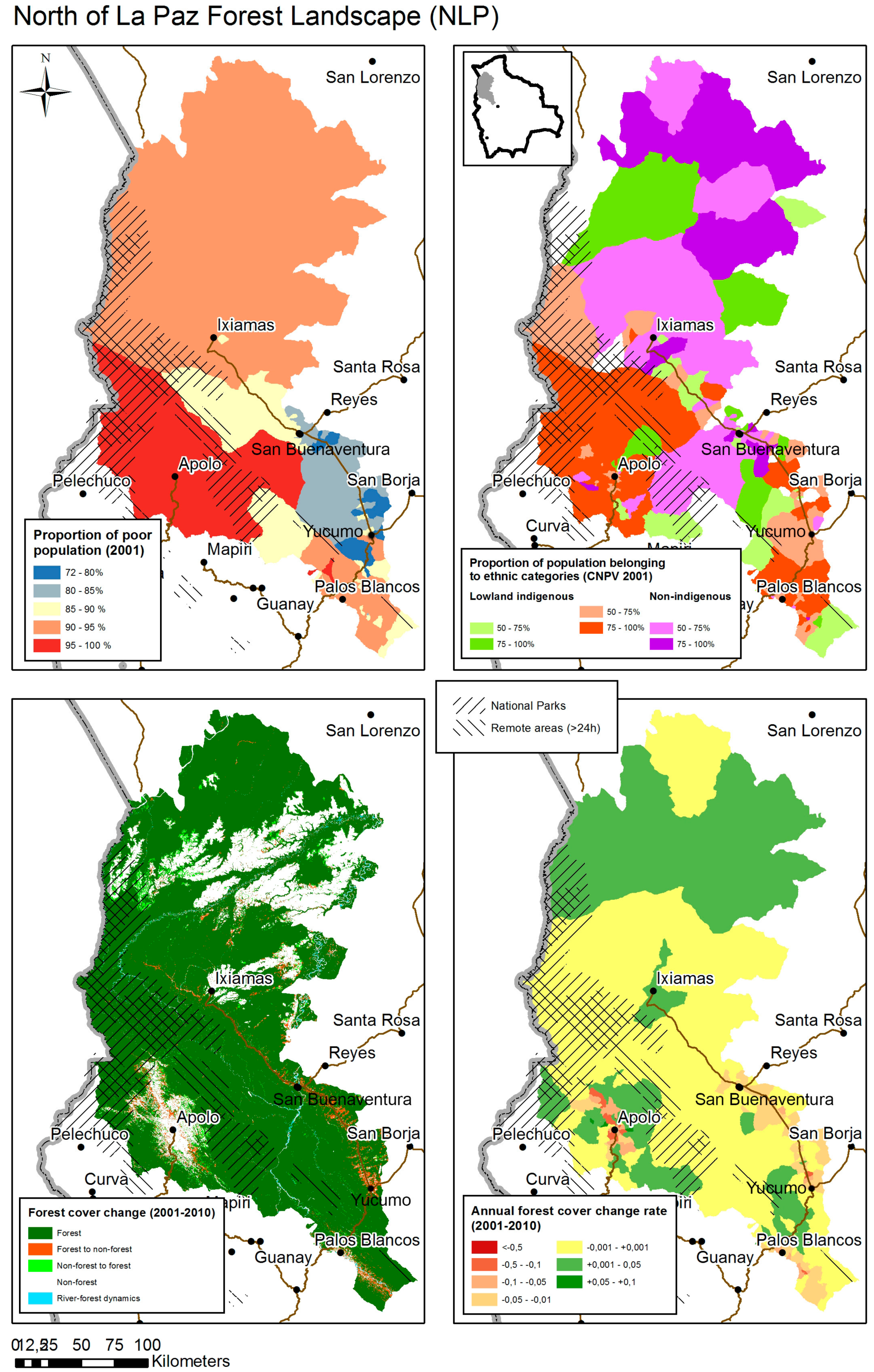
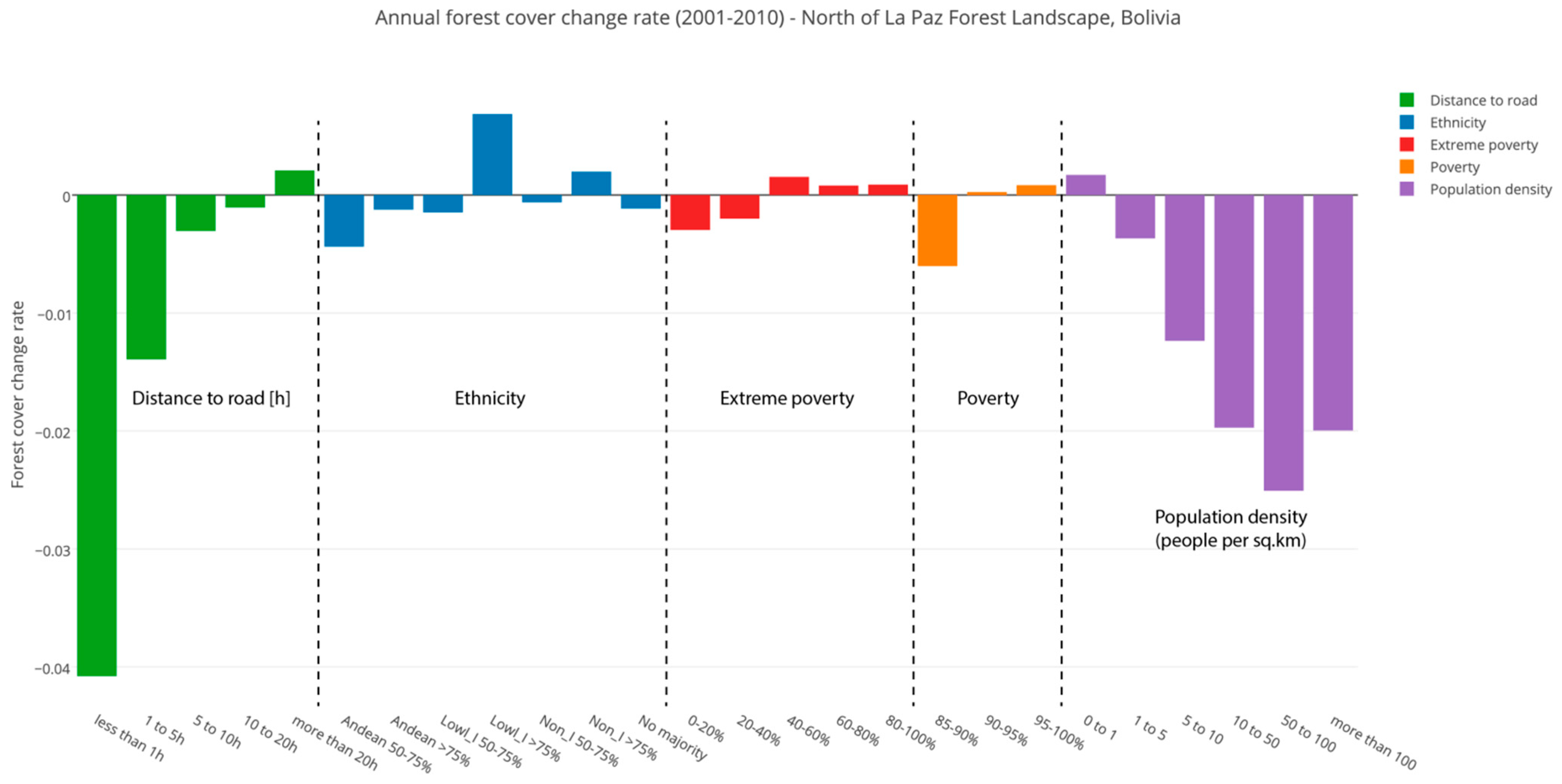
2.2.1. The North of La Paz Forest Landscape (NLP)

In the NLP case (Figure 3), two hotspots of forest conversion are visible. The first one, along the road from Palos Blancos to Ixiamas, is a colonization area opened after 1983, and settled mainly by Andean groups, but also by some mestizo and lowland indigenous people. The other spot is found around the town of Apolo, where forests are being converted to grasslands and shrub, and possibly coca [68]. This area is inhabited mainly by Andean indigenous people and has very high levels of poverty. This explains the negative forest balance in areas dominated by Andean people (Figure 4), as well as the positive correlations between Andean population and forest loss (Table 4). There, forest loss is part of the ongoing colonization process and development of agriculture related to local and national markets. Figure 4 also shows increasing negative forest balance with population density, with a peak at 50 to 100 inhabitants per km², and decreasing forest loss with distance to road. Net forest gain occurs only at very low population densities and in very remote areas. Travel time to roads, local and urban centers has a negative relationship with forest loss (Table 4).

Forest gain occurs in the North of the area and might correspond to regeneration of pastures to forest, but should be confirmed by field observations difficult to get in this extremely remote area. This area is inhabited by sparse lowland indigenous people and mestizo cattle ranchers, thus explaining the positive forest balance for areas inhabited by these groups, and the negative correlation between non- indigenous people and forest loss (Table 4). Both forest loss and gain correlates positively with poverty and extreme poverty (Table 4). On the one hand, poor Andean communities near roads convert forest, but on the other hand, forest increases in the poorest communities located further away along the road and around Apolo and Ixiamas and in the far North of the area (Figure 3). The co-occurrence of forest loss and gain in the poorest and more remote communities might correspond to shifting cultivation and fallows practiced by both Andean and Lowland indigenous peoples.

The observed changes in the NLP area are in line with the findings of case studies in the area. The colonization area along the road Yucumo-San Buenaventura corresponds to the area studied by Bottazzi and Dao [40], who showed that forest loss decreased with road distance, with private properties being established near the road and common properties further away. Forrest et al. [69] observed an expansion of grasslands around Apolo, and forest increase in more remote areas and within Madidi National Park. In his study area around Ixiamas, Sandoval [70] observed forest increase between 2001 and 2010, which he relates with secondary forest development on fallow land and flooded areas. Locklin and Haack [71] and Killeen et al. [36], mention the importance of fallow in Andean colonist land management systems, as well as some cases of land abandonment by settlers who migrated to urban areas or returned to their communities of origin.

Figure 3. Poverty, ethnic groups and forest cover change in the North of La Paz forest landscape.

Figure 3. Poverty, ethnic groups and forest cover change in the North of La Paz forest landscape.

Figure 4. Forest cover change rate in relation with socio-economic variables in the North of La Paz forest landscape (NLP).

Figure 4. Forest cover change rate in relation with socio-economic variables in the North of La Paz forest landscape (NLP).

Table 4. Pearson correlations between forest cover change and socio-economic variables in the North of La Paz forest landscape.

	Forest Cover %	Forest Cover %	Forest Loss	Forest Gain
	(2001)	(2010)	(2001–2010)	(2001–2010)
Population density	−0.020	−0.073 **	0.249 **	0.023
Poverty rate (%)	−0.206 **	−0.164 **	0.170 **	0.203 **
Extreme poverty rate (%)	−0.146 **	−0.130 **	0.265 **	0.216 **
Travel time to main road	−0.057 **	0.022	−0.266 **	0.031
Travel time to district capital	−0.037 *	0.043 *	−0.276 **	0.036
Travel time to province capital	−0.146 **	−0.066 **	−0.220 **	0.054 **
Travel time to nearest community	0.139 **	0.195 **	−0.234 **	−0.039 *
Andean population (%)	0.124 **	0.083 **	0.250 **	0.078 **
Lowland indigenous population (%)	−0.125 **	−0.083 **	−0.046 *	0.153 **
Non-indigenous population (%)	0.000	0.000	−0.192**	−0.216 **

** The correlation is significant at 0.01 level (2-tailed); * The correlation is significant at 0.05 level (2-tailed).

Table 4. Pearson correlations between forest cover change and socio-economic variables in the North of La Paz forest landscape.

	Forest Cover %	Forest Cover %	Forest Loss	Forest Gain
	(2001)	(2010)	(2001–2010)	(2001–2010)
Population density	−0.020	−0.073 **	0.249 **	0.023
Poverty rate (%)	−0.206 **	−0.164 **	0.170 **	0.203 **
Extreme poverty rate (%)	−0.146 **	−0.130 **	0.265 **	0.216 **
Travel time to main road	−0.057 **	0.022	−0.266 **	0.031
Travel time to district capital	−0.037 *	0.043 *	−0.276 **	0.036
Travel time to province capital	−0.146 **	−0.066 **	−0.220 **	0.054 **
Travel time to nearest community	0.139 **	0.195 **	−0.234 **	−0.039 *
Andean population (%)	0.124 **	0.083 **	0.250 **	0.078 **
Lowland indigenous population (%)	−0.125 **	−0.083 **	−0.046 *	0.153 **
Non-indigenous population (%)	0.000	0.000	−0.192**	−0.216 **

** The correlation is significant at 0.01 level (2-tailed); * The correlation is significant at 0.05 level (2-tailed).

Multivariate models (Table 5 and Table 6) show that accessibility and extreme poverty are determinants of both forest loss and gain. While Andean people also determine forest loss, it has a negative relationship with gain. Lowland indigenous peoples determine gain, and non-indigenous peoples have a negative relationship with loss. A possible interpretation is that both forest gain and loss might occur in areas with middle remoteness inhabited by lowland indigenous peoples and some Andean colonists. Forest losses occur then in Andean colonist’s areas with good access but a high incidence of poverty. Communities of mestizo cattle ranchers, located further away, experience little change in forest cover.

Table 5. Significance of explanatory variables for relative forest loss in the multivariate stepwise regression model.

	NLP	NLP	SCA	SCA	SCA	LPP	LPP	LNP	LNP
	Loss	Loss	Loss	Loss	Loss	Loss	Loss	Loss	Loss
L_Population density	(L_Droad)	(L_Droad)	(L_Droad)	(L_Droad)	(L_Droad)	(L_Droad)	(L_dep)	(L_Droad)	(L_vil)
Poverty	(Extr.pov)	(Extr.pov)	(Extr.pov)	(Extr.pov)	(Extr.pov)	** (+)	n/s	n/s	n/s
Extreme poverty	*** (+)	*** (+)	n/s	n/s	n/s	N/A	N/A	N/A	N/A
L_Droad	*** (−)	*** (−)	*** (−)	*** (−)	*** (−)	*** (−)	(L_dep)	*** (−)	(L_vil)
L_Dmun_distr	(L_Droad)	(L_Droad)	(L_Droad)	(L_Droad)	(L_Droad)	(L_Droad)	(L_dep)	(L_Droad)	(L_vil)
L_Ddep_prov	(L_Droad)	(L_Droad)	(L_Droad)	(L_Droad)	(L_Droad)	(L_Droad)	*** (+)	(L_Droad)	(L_vil)
L_Dvillage	(L_Droad)	(L_Droad)	(L_Droad)	(L_Droad)	(L_Droad)	(L_Droad)	(L_dep)	(L_Droad)	*** (−)
P_Andean	** (+)	(P_NonI)	*** (+)	(P_Noi)	*** (+)	N/A	N/A	N/A	N/A
P_LowlI	(P_And)	n/s	*** (−)	*** (−)	(P_Noi)	N/A	N/A	N/A	N/A
P_NonI	(P_And)	*** (−)	(P_And)	*** (−)	*** (+)	N/A	N/A	N/A	N/A
P_TaiK	N/A	N/A	N/A	N/A	N/A	n/s	* (-)	** (+)	* (+)
P_Austas	N/A	N/A	N/A	N/A	N/A	(P_TaiK)	(P_Taik)	n/s	n/s
P_MiaoTib	N/A	N/A	N/A	N/A	N/A	** (−)	* (−)	(P_Austr)	(P_Austr)

*** = significant at 0 < p < 0.001; ** = significant at 0.001 < p < 0.01; * = significant at 0.01 < p < 0.05; =significant at 0.05 < p < 0.1; n/s = not significant. The signs indicate the correlation direction. Indications between parenthesis show the variables to which to not used variables were correlated at >0.5. L_x indicate the 10-base log of the variable.

Table 5. Significance of explanatory variables for relative forest loss in the multivariate stepwise regression model.

	NLP	NLP	SCA	SCA	SCA	LPP	LPP	LNP	LNP
	Loss	Loss	Loss	Loss	Loss	Loss	Loss	Loss	Loss
L_Population density	(L_Droad)	(L_Droad)	(L_Droad)	(L_Droad)	(L_Droad)	(L_Droad)	(L_dep)	(L_Droad)	(L_vil)
Poverty	(Extr.pov)	(Extr.pov)	(Extr.pov)	(Extr.pov)	(Extr.pov)	** (+)	n/s	n/s	n/s
Extreme poverty	*** (+)	*** (+)	n/s	n/s	n/s	N/A	N/A	N/A	N/A
L_Droad	*** (−)	*** (−)	*** (−)	*** (−)	*** (−)	*** (−)	(L_dep)	*** (−)	(L_vil)
L_Dmun_distr	(L_Droad)	(L_Droad)	(L_Droad)	(L_Droad)	(L_Droad)	(L_Droad)	(L_dep)	(L_Droad)	(L_vil)
L_Ddep_prov	(L_Droad)	(L_Droad)	(L_Droad)	(L_Droad)	(L_Droad)	(L_Droad)	*** (+)	(L_Droad)	(L_vil)
L_Dvillage	(L_Droad)	(L_Droad)	(L_Droad)	(L_Droad)	(L_Droad)	(L_Droad)	(L_dep)	(L_Droad)	*** (−)
P_Andean	** (+)	(P_NonI)	*** (+)	(P_Noi)	*** (+)	N/A	N/A	N/A	N/A
P_LowlI	(P_And)	n/s	*** (−)	*** (−)	(P_Noi)	N/A	N/A	N/A	N/A
P_NonI	(P_And)	*** (−)	(P_And)	*** (−)	*** (+)	N/A	N/A	N/A	N/A
P_TaiK	N/A	N/A	N/A	N/A	N/A	n/s	* (-)	** (+)	* (+)
P_Austas	N/A	N/A	N/A	N/A	N/A	(P_TaiK)	(P_Taik)	n/s	n/s
P_MiaoTib	N/A	N/A	N/A	N/A	N/A	** (−)	* (−)	(P_Austr)	(P_Austr)

*** = significant at 0 < p < 0.001; ** = significant at 0.001 < p < 0.01; * = significant at 0.01 < p < 0.05; =significant at 0.05 < p < 0.1; n/s = not significant. The signs indicate the correlation direction. Indications between parenthesis show the variables to which to not used variables were correlated at >0.5. L_x indicate the 10-base log of the variable.

Table 6. Significance of explanatory variables for relative forest gain in the multivariate stepwise regression model.

	NLP	NLP	SCA	SCA	SCA	LPP	LPP	LNP	LNP
	Gain	Gain	Gain	Gain	Gain	Gain	Gain	Gain	Gain
L_Population density	(L_Droad)	(L_Droad)	(L_Droad)	(L_Droad)	(L_Droad)	(L_Droad)	(L_vil)	(L_Droad)	(L_vil)
Poverty	(Extr.pov)	(Extr.pov)	(Extr.pov)	(Extr.pov)	(Extr.pov)	n/s	n/s	n/s	n/s
Extreme poverty	*** (+)	*** (+)	*** (+)	*** (+)	*** (+)	N/A	N/A	N/A	N/A
L_Droad	*** (−)	*** (−)	*** (−)	*** (−)	*** (−)	* (+)	(L_vil)	n/s	(L_vil)
L_Dmun_distr	(L_Droad)	(L_Droad)	(L_Droad)	(L_Droad)	(L_Droad)	(L_Droad)	(L_vil)	(L_Droad)	(L_vil)
L_Ddep_prov	(L_Droad)	(L_Droad)	(L_Droad)	(L_Droad)	(L_Droad)	(L_Droad)	(L_vil)	(L_Droad)	(L_vil)
L_Dvillage	(L_Droad)	(L_Droad)	(L_Droad)	(L_Droad)	(L_Droad)	(L_Droad)	** (+)	(L_Droad)	n/s
P_Andean	*** (−)	(P_NonI)	*** (+)	(P_Noi)	n/s	N/A	N/A	N/A	N/A
P_LowlI	(P_And)	*** (+)	*** (+)	n/s	(P_Noi)	N/A	N/A	N/A	N/A
P_NonI	(P_And)	* (−)	(P_And)	*** (−)	*** (−)	N/A	N/A	N/A	N/A
P_TaiK	N/A	N/A	N/A	N/A	N/A	*** (−)	*** (−)	* (−)	* (−)
P_Austas	N/A	N/A	N/A	N/A	N/A	(P_TaiK)	(P_Taik)	n/s	n/s
P_MiaoTib	N/A	N/A	N/A	N/A	N/A	n/s	n/s	(P_Austr)	(P_Austr)

*** = significant at 0 < p < 0.001; ** = significant at 0.001 < p < 0.01; * = significant at 0.01 < p < 0.05; =significant at 0.05 < p < 0.1; n/s = not significant; The signs indicate the correlation direction. Indications between parenthesis show the variables to which to not used variables were correlated at >0.5; L_x indicate the 10-base log of the variable.

Table 6. Significance of explanatory variables for relative forest gain in the multivariate stepwise regression model.

	NLP	NLP	SCA	SCA	SCA	LPP	LPP	LNP	LNP
	Gain	Gain	Gain	Gain	Gain	Gain	Gain	Gain	Gain
L_Population density	(L_Droad)	(L_Droad)	(L_Droad)	(L_Droad)	(L_Droad)	(L_Droad)	(L_vil)	(L_Droad)	(L_vil)
Poverty	(Extr.pov)	(Extr.pov)	(Extr.pov)	(Extr.pov)	(Extr.pov)	n/s	n/s	n/s	n/s
Extreme poverty	*** (+)	*** (+)	*** (+)	*** (+)	*** (+)	N/A	N/A	N/A	N/A
L_Droad	*** (−)	*** (−)	*** (−)	*** (−)	*** (−)	* (+)	(L_vil)	n/s	(L_vil)
L_Dmun_distr	(L_Droad)	(L_Droad)	(L_Droad)	(L_Droad)	(L_Droad)	(L_Droad)	(L_vil)	(L_Droad)	(L_vil)
L_Ddep_prov	(L_Droad)	(L_Droad)	(L_Droad)	(L_Droad)	(L_Droad)	(L_Droad)	(L_vil)	(L_Droad)	(L_vil)
L_Dvillage	(L_Droad)	(L_Droad)	(L_Droad)	(L_Droad)	(L_Droad)	(L_Droad)	** (+)	(L_Droad)	n/s
P_Andean	*** (−)	(P_NonI)	*** (+)	(P_Noi)	n/s	N/A	N/A	N/A	N/A
P_LowlI	(P_And)	*** (+)	*** (+)	n/s	(P_Noi)	N/A	N/A	N/A	N/A
P_NonI	(P_And)	* (−)	(P_And)	*** (−)	*** (−)	N/A	N/A	N/A	N/A
P_TaiK	N/A	N/A	N/A	N/A	N/A	*** (−)	*** (−)	* (−)	* (−)
P_Austas	N/A	N/A	N/A	N/A	N/A	(P_TaiK)	(P_Taik)	n/s	n/s
P_MiaoTib	N/A	N/A	N/A	N/A	N/A	n/s	n/s	(P_Austr)	(P_Austr)

*** = significant at 0 < p < 0.001; ** = significant at 0.001 < p < 0.01; * = significant at 0.01 < p < 0.05; =significant at 0.05 < p < 0.1; n/s = not significant; The signs indicate the correlation direction. Indications between parenthesis show the variables to which to not used variables were correlated at >0.5; L_x indicate the 10-base log of the variable.

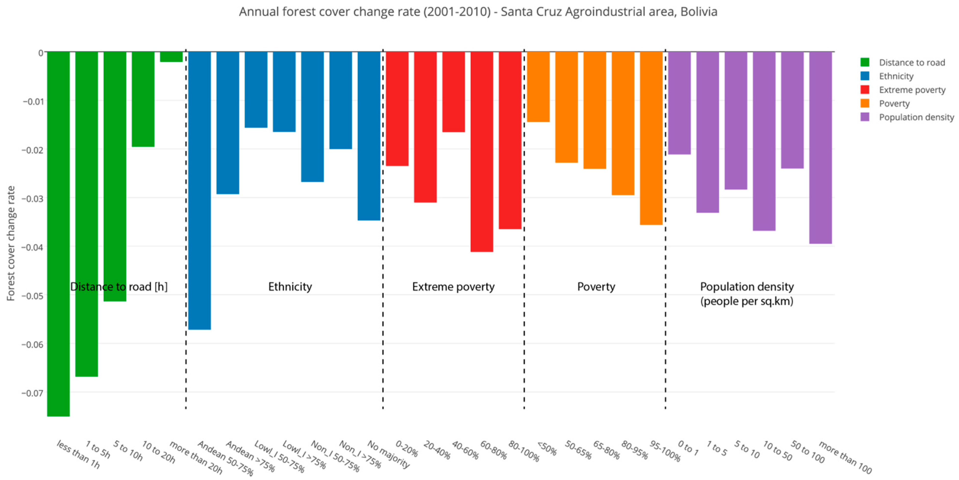
2.2.2. The Santa Cruz Agroindustrial Area (SCA)

The SCA case shows negative forest cover balance for all population density, poverty, ethnicity and accessibility categories (Figure 5). Forest conversion follows a radial expansion around the city of Santa Cruz and along penetration roads to the North. At the East and North-West, a mosaic of large plots of forest clearings is visible, which correspond to the main area of agroindustrial farming. In the Western and Northern areas, the plots are smaller and show fishbone-like deforestation similar to the NLP case. Areas of forest gain are visible in the most remote areas, in areas inhabited by lowland indigenous people in the North-East (San Javier), in Andean colonization areas around San Julian, and in area inhabited by Mestizos along the Rio Grande River.

Figure 5. Poverty, ethnic groups and forest cover change in the Santa Cruz agroindustrial area.

Figure 5. Poverty, ethnic groups and forest cover change in the Santa Cruz agroindustrial area.

Like in the NLP case, distance to roads, local and urban centers correlate negatively with forest loss (Table 7), and forest loss rate (Figure 6). Additionally, we observe a decrease of forest gain with remoteness (Table 7). These relationships are confirmed in the multivariate models, with accessibility as a highly significant determinant of forest loss as well as forest gain. Also like in the NLP case, areas inhabited by Andean settlers show the highest forest loss rate (Figure 6) and their population proportion correlate with forest loss (Table 7). A high forest loss rate is also observed in ethnically mixed communities (Table 7). In the multivariate model, Andean population determines both forest loss and gain, while lowland indigenous peoples have a positive relationship with forest gain and negative with loss. Extreme poverty has a positive relationship with loss and gain (Table 5 and Table 6), showing increasing loss rates at higher poverty levels. However, poverty appears not to be a significant determinant of forest loss in the multivariate model, yet does with forest gain. Surprisingly, the presence of non-indigenous population has a negative relationship with forest loss, as well as with forest gain. In the multivariate model their relation with forest loss is ambiguous, being in one model a positive and in another a negative driver.

Table 7. Pearson correlations between forest cover change and socio-economic variables in the Santa Cruz agro industrial area.

	Forest Cover %	Forest Cover %	Forest Loss	Forest Gain
	(2001)	(2010)	(2001–2010)	(2001–2010)
Population density	−0.340 **	−0.286 **	0.218 **	0.138 **
Poverty rate (%)	−0.074 **	−0.099 **	0.090 **	0.159 **
Extreme poverty rate (%)	−0.253 **	−0.243 **	0.167 **	0.234 **
Travel time to main road	0.494 **	0.569 **	−0.441 **	−0.159 **
Travel time to district capital	0.508 **	0.579 **	−0.448 **	−0.175 **
Travel time to province capital	0.523 **	0.582 **	−0.441 **	−0.162 **
Travel time to nearest community	0.492 **	0.570 **	−0.442 **	−0.179 **
Andean population (%)	−0.111 **	−0.214 **	0.256 **	0.134 **
Lowland indigenous population (%)	0.029	0.078 **	−0.127 **	0.070 **
Non-indigenous population (%)	0.071 **	0.120 **	−0.118 **	−0.166 **

** The correlation is significant at 0.01 level (2-tailed); * The correlation is significant at 0.05 level (2-tailed).

Table 7. Pearson correlations between forest cover change and socio-economic variables in the Santa Cruz agro industrial area.

	Forest Cover %	Forest Cover %	Forest Loss	Forest Gain
	(2001)	(2010)	(2001–2010)	(2001–2010)
Population density	−0.340 **	−0.286 **	0.218 **	0.138 **
Poverty rate (%)	−0.074 **	−0.099 **	0.090 **	0.159 **
Extreme poverty rate (%)	−0.253 **	−0.243 **	0.167 **	0.234 **
Travel time to main road	0.494 **	0.569 **	−0.441 **	−0.159 **
Travel time to district capital	0.508 **	0.579 **	−0.448 **	−0.175 **
Travel time to province capital	0.523 **	0.582 **	−0.441 **	−0.162 **
Travel time to nearest community	0.492 **	0.570 **	−0.442 **	−0.179 **
Andean population (%)	−0.111 **	−0.214 **	0.256 **	0.134 **
Lowland indigenous population (%)	0.029	0.078 **	−0.127 **	0.070 **
Non-indigenous population (%)	0.071 **	0.120 **	−0.118 **	−0.166 **

** The correlation is significant at 0.01 level (2-tailed); * The correlation is significant at 0.05 level (2-tailed).

Case studies from the SCA area link the ongoing deforestation process with the expansion of agroindustrial areas. Large farms are usually owned by mestizo or European-descent Bolivians, or foreginers [39]. Agroindustrial expansion responds to the demand of Andean community countries for soybeans [39], which accounted for 52% of cropland area in the Santa Cruz department in 2009 [72]. This “soybean boom” is being increasingly controlled by Brazilian agroindustrial companies, which purchase land with the help of local brokers, leading to large-scale land appropriation and concentration, encroaching into smallholders’ and forest land and converting their former owners into wage workers, while residing in urban areas of Bolivia or Brazil [72,73]. Taking these data into account, high forest losses observed in communities dominated by Andean settlers with high poverty rates do not necessarily mean that these communities are controlling land use changes in the area. The co-existence of high poverty rates and large patches of forest clearings (which are only possible with mechanized technology) reveal highly unequal relationships in terms of land control, and a probable disempowerment of indigenous and Andean communities linked with the agroindustrial expansion.

Figure 6. Forest cover change rate in relation with socio-economic variables in the Santa Cruz agroindustrial area (SCA).

Figure 6. Forest cover change rate in relation with socio-economic variables in the Santa Cruz agroindustrial area (SCA).

Agroindustrialists also react to national land policies: Redo et al. [39] showed that some large landowners have cleared more forest after 2006 to provide proof of use and avoid the perceived risk of expropiation by the State under the “socio-economic function” amendment. On the other hand, the afflux of migrants from the Bolivian highlands, either spontaneous or supported by the government increased and might have driven accelerated forest conversion in the San Julian area between 2001 and 2006 shows [74]. Finally, two case studies [39,74] mention the disastrous floods of 2006–2007 which led to land abandonment along the Rio Grande, thus possibly explaining vegetation increase in this area until 2010.

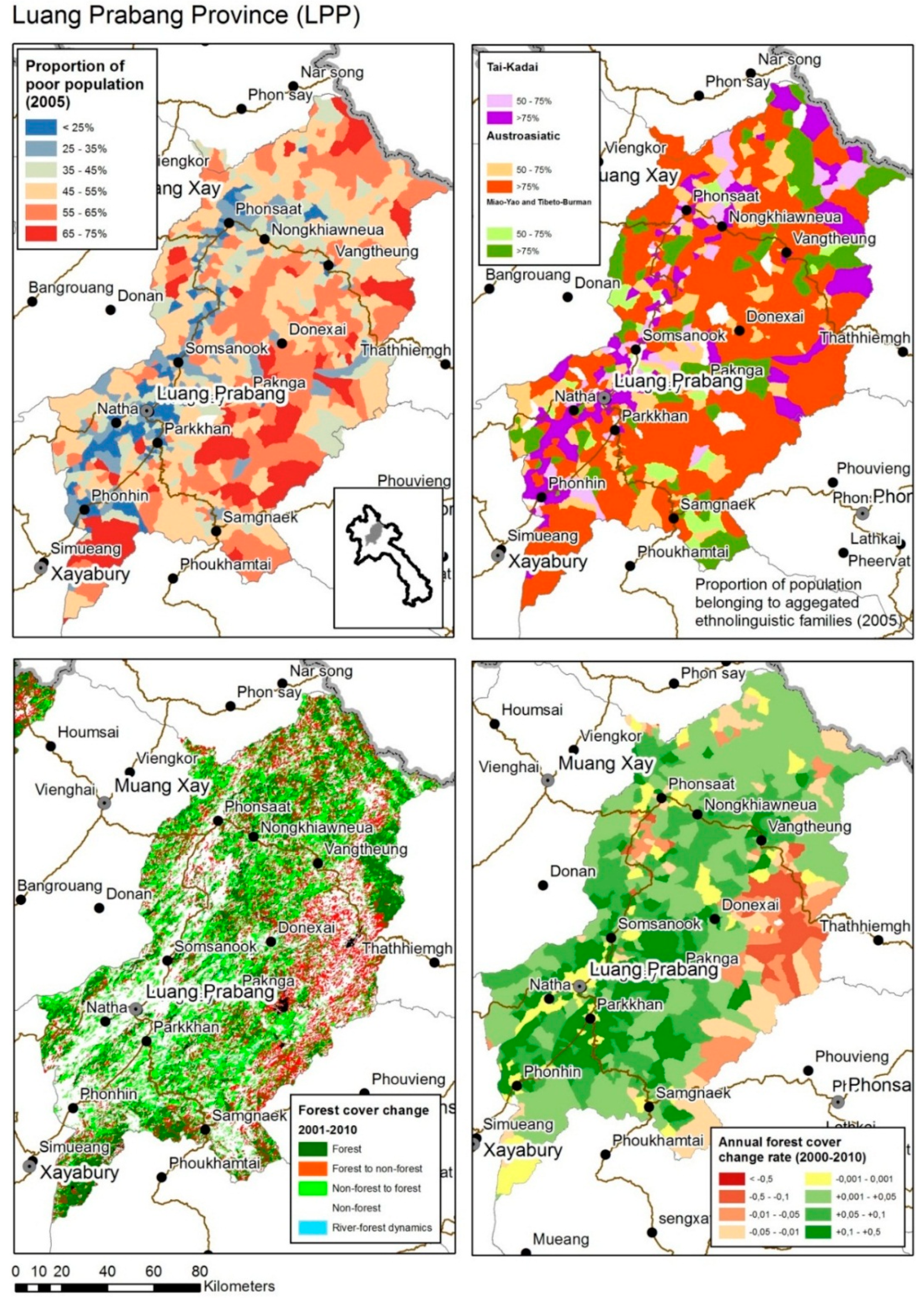
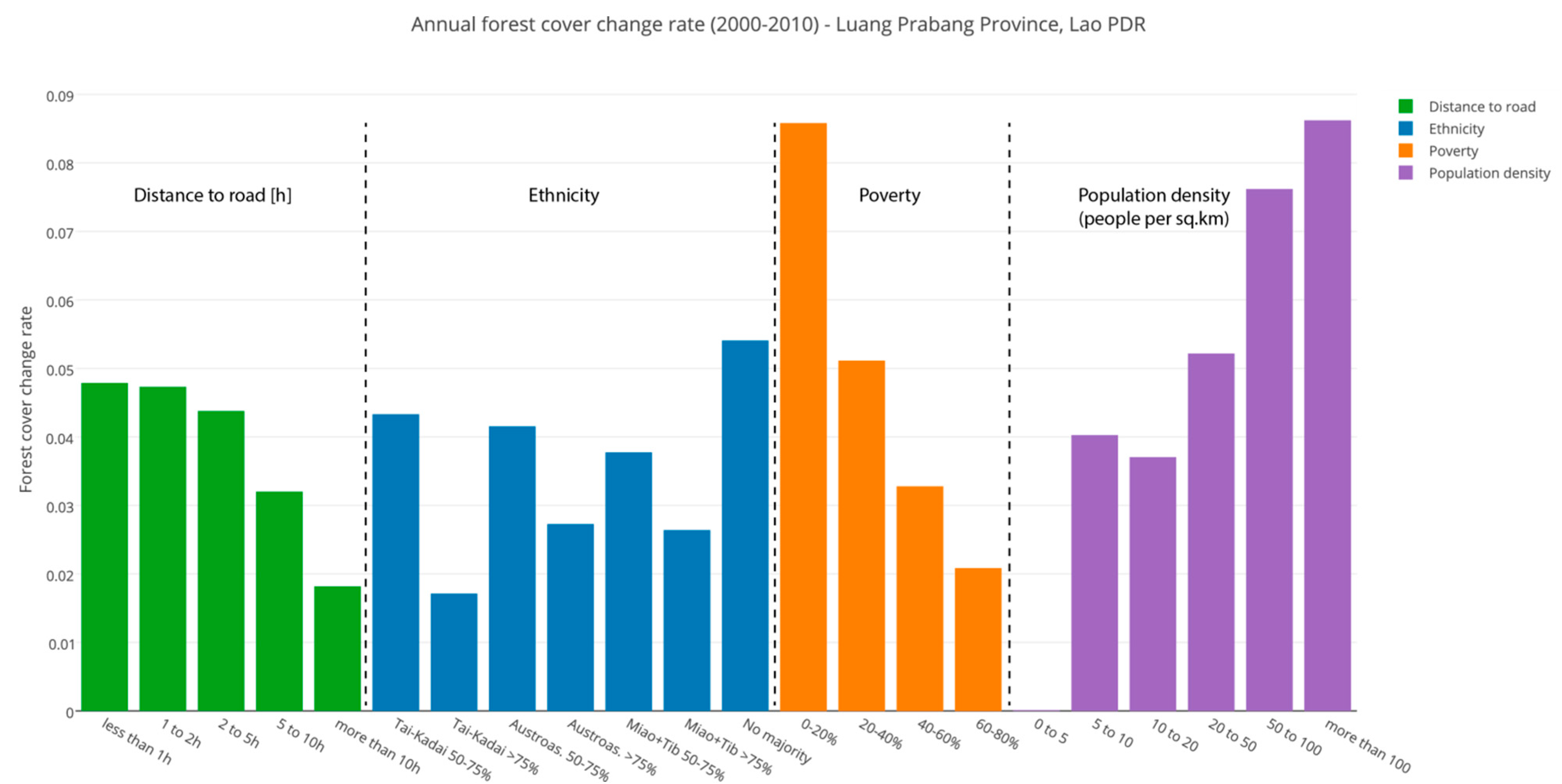
2.2.3. The Luang Prabang Province (LPP)

Contrary to the other study areas, the Luang Prabang province has experienced more forest gain than loss and shows an overall positive forest balance. Forest gain occurred in the whole area but more specifically in the mountainous areas East of the city of Luang Prabang. Forest loss is concentrated in the Far East of the province (Figure 7). Both forest gain and loss show a patchy pattern, typical for shifting cultivation. This landscape dynamic is challenging to interpret because the spatial resolution of 30 m does not allow to capture most small-scale cultivation plots, the distinction between shrub and secondary forest is gradual and difficult to classify, and there is a strong influence of topography (shadows and semi-shadows) on spectral signature. Therefore, these results must be interpreted with caution and in relative more than in absolute terms.

Despite the possible forest loss hotspot at the eastern border of the province, all socio-economic categories are associated with forest increase (Figure 8). Forest gain is higher near roads, at high population densities, in ethnic Lao dominated or ethnically mixed communities, and in communities with lower poverty rate. However, no significant correlations could be found between these variables and forest gain. Furthermore, the multivariate model shows however a decreasing of forest gain with proportion of ethnic Lao. Contrary to the other study areas, forest loss increases with distance to district and province capitals, in simple correlations (Table 8) and also in the multivariate model (Table 5 and Table 6). However, in the multivariate model, forest loss decreases with road distance. Forest loss correlates with Austroasiatic population proportion, and in the models, the proportion of other minorities (Miao-Yao and Tibeto-Burman) predicts a decrease of forest loss. Finally, more remote areas also have a higher baseline forest cover (Table 8).

Figure 7. Poverty, ethnic groups and forest cover change in the Luang Prabang province.

Figure 7. Poverty, ethnic groups and forest cover change in the Luang Prabang province.

Figure 8. Forest cover change rate in relation with socio-economic variables in the Luang Prabang province (LPP).

Figure 8. Forest cover change rate in relation with socio-economic variables in the Luang Prabang province (LPP).

Table 8. Pearson correlations between forest cover change and socio-economic variables in the Luang Prabang Province.

	Forest Cover %	Forest Cover %	Forest Loss	Forest Gain
	(2001)	(2010)	(2000–2010)	(2000–2010)
Population density	−0.454 **	−0.323 **	−0.021	−0.104 **
Poverty rate (%)	0.361 **	0.239 **	0.085 **	0.087 **
Travel time to main road	0.497 **	0.330 **	−0.052	0.012
Travel time to district capital	0.502 **	0.277 **	0.078 **	0.047
Travel time to province capital	0.527 **	0.264**	0.159 **	0.034
Travel time to nearest village	0.550 **	0.328 **	−0.067 *	−0.042
Tai-Kadai population (%)	−0.094 **	−0.117 **	−0.084 **	−0.146 **
Austroasiatic population (%)	0.074 *	0.032	0.116 **	0.074 *
Miao-Yao and Tibeto-Burman population (%)	0.001	0.075 *	−0.059	0.053

** The correlation is significant at 0.01 level (2-tailed); * The correlation is significant at 0.05 level (2-tailed).

Table 8. Pearson correlations between forest cover change and socio-economic variables in the Luang Prabang Province.

	Forest Cover %	Forest Cover %	Forest Loss	Forest Gain
	(2001)	(2010)	(2000–2010)	(2000–2010)
Population density	−0.454 **	−0.323 **	−0.021	−0.104 **
Poverty rate (%)	0.361 **	0.239 **	0.085 **	0.087 **
Travel time to main road	0.497 **	0.330 **	−0.052	0.012
Travel time to district capital	0.502 **	0.277 **	0.078 **	0.047
Travel time to province capital	0.527 **	0.264**	0.159 **	0.034
Travel time to nearest village	0.550 **	0.328 **	−0.067 *	−0.042
Tai-Kadai population (%)	−0.094 **	−0.117 **	−0.084 **	−0.146 **
Austroasiatic population (%)	0.074 *	0.032	0.116 **	0.074 *
Miao-Yao and Tibeto-Burman population (%)	0.001	0.075 *	−0.059	0.053

** The correlation is significant at 0.01 level (2-tailed); * The correlation is significant at 0.05 level (2-tailed).

These results have to be interpreted in relation with the well documented diminishment of shifting agriculture in the area, a widespread phenomenon throughout Southeast Asia [75]. Luang Prabang is the area in Northern Laos which experienced the most dramatic decrease, with total area covered by shifting cultivation landscapes declining from 56.3% to 39.8% between the periods 2000–2006 and 2003–2009 [76]. This change came along with an increase of intensive agriculture in four Northern Lao provinces, as well as forest increase already observed between 1997 to 2000, and attributed to abandoned shifting cultivation areas, which are however difficult to distinguish from used fallow and shrub [77]. The decline of shifting cultivation might be especially strong in LPP because the province was among the first to implement LUPLA and village resettlement policies, aimed at reducing this practice, among other objectives [46,77]. Resettlements have particularly affected ethnic minorities, and among them the Hmong who belong to the Miao-Yao family. The positive relations between forest loss with remoteness, high poverty levels and the presence of Austroasiatic ethnic groups is to be related with the persistence of shifting cultivation practices [54]. Austroasiatic peoples have the largest share of their area covered by shifting cultivation landscapes [54], and their management practices tend to favor secondary forests from where they collect non-timber products [78].

With these considerations, we interpret the observed forest increase as secondary forest regrowth on abandoned shifting cultivation plots linked with policies aiming at reducing this land use practice. These policies are likely to be more strongly implemented in easily accessible areas, and in relocated areas, which are characterized by ethnic mix, better access to services but also an increase in population density, as observed in the LPP area [55,79].

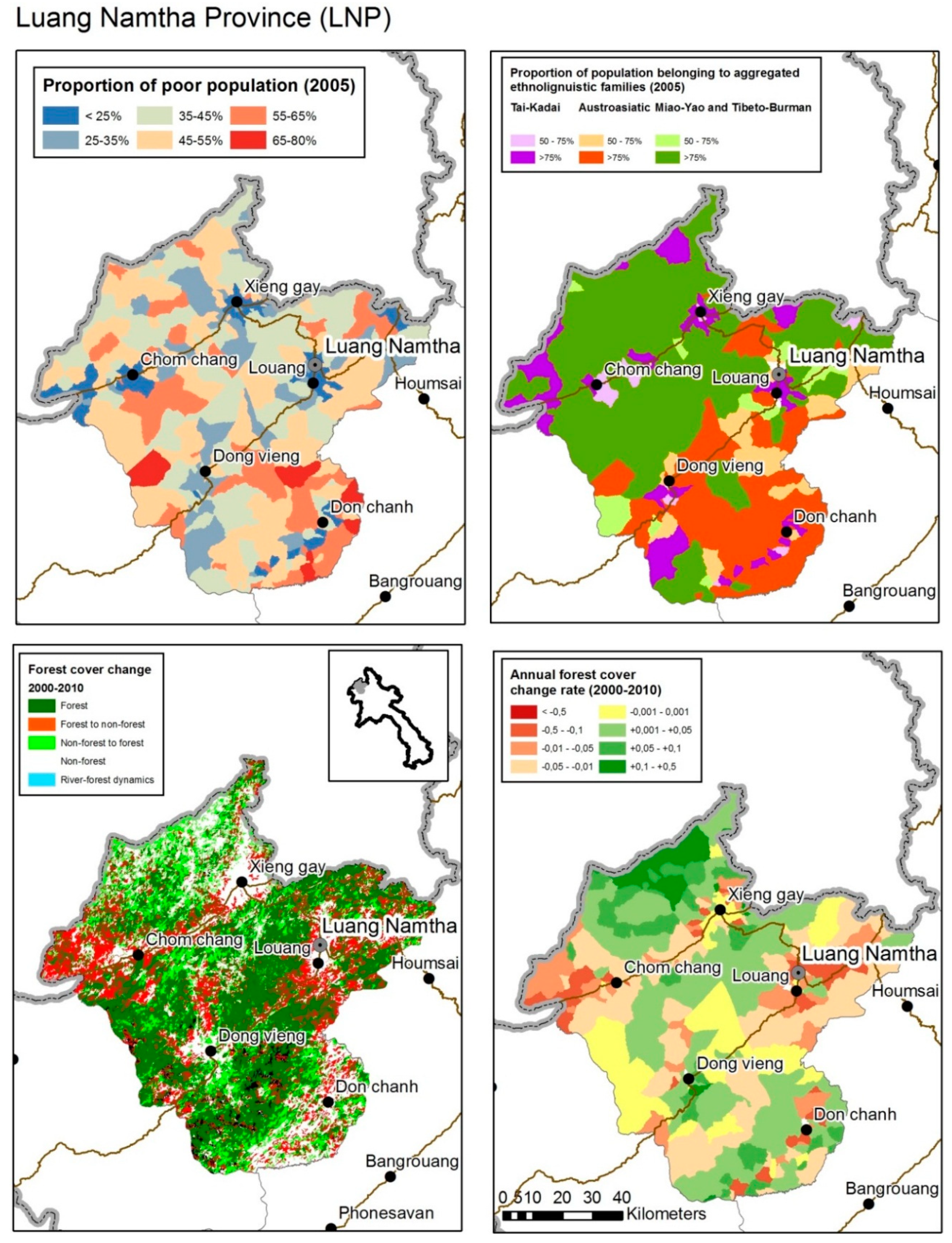
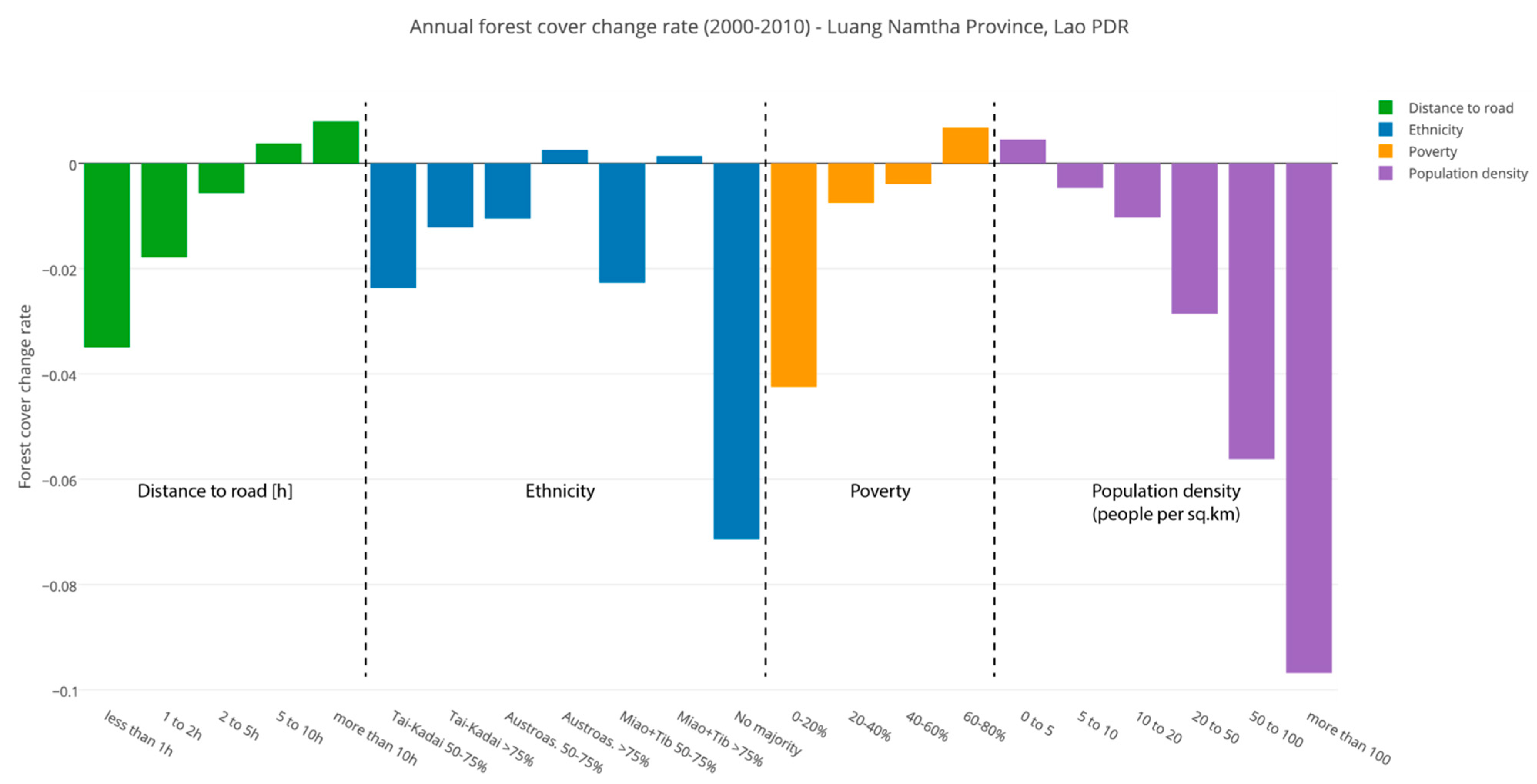
2.2.4. The Luang Namtha Province (LNP)

The case of Luang Namtha province shows an overall loss in forest, concentrated mainly along the roads which connect China to Myanmar and Thailand, and around the urban centers of Luang Namtha and Dong Vieng (Figure 9). Smaller forest conversion patches can be observed together with forest gain areas in the far North and South of the province.

Forest loss has a positive relation with population density and accessibility to roads and is concentrated in communities with a population density of more than 20 people/km² and at less than 2 h of travel from main roads (Figure 10). These trends are also visible in bivariate correlations (Table 9) and the multivariate models (Table 5 and Table 6). Inversely, forest gain increases with distance. Communities with more than 75% of population belonging to Austoasiatic, Miao-Yao or Tibeto-Burman families have a slightly positive forest cover change rate. On the other hand, the communities with the highest forest loss rate are the ethnically mixed ones, and the ones dominated by ethnic Lao, or Tibeto-Burman. The proportion of ethnic Lao correlates positively with forest loss and negatively with forest gain, in both bivariate correlations (Table 9) and multivariate models (Table 5 and Table 6). The area also shows differenced forest cover change related with poverty: less poor areas experience higher forest loss rates, while the poorest communities—often also dominated by ethnic minorities as shown in Table 9—are gaining forest.

The province of Luang Namtha experienced a large expansion of rubber plantations [80] after the opening of trade with China and Thailand and the growth of Chinese demand after 2003, and thanks to its strategic location along two main roads which link China to Thailand and Myanmar. Rubber was also promoted by the government as an alternative to opium poppy cultivation [81]. With a growing involvement of Chinese investors and companies, the area of rubber cultivation in LNP grew from 300 ha in 2002 to more than 30,000 in 2012 [57]. Rubber is usually planted by smallholders, freely or under contract with Chinese investors, on former shifting cultivation fields [57,77]. Thongmanivong et al. [82] observed that the replacement of shifting cultivation areas with rubber came along with a directed and then spontaneous migration of upland communities along the roads, especially the Akha, who belong to the Tibeto-Burman ethnolinguistic family. Their analysis shows that some Akha have relatives in China and used their network to start rubber plantations, as also do the ethnic Lao. These authors also found an increase in upland agriculture, though the production of upland rice has declined. Hurni et al. [76] observed an increase of patchy forest clearings in the province, which they attribute to young rubber plantations. Considering this analysis and the fact that rubber trees become only productive after 7 years [76] it seems that rubber planters are mainly wealthier people and communities able to invest, while poorer people lease their lands or migrate out of their villages as wage laborers [82]. With these considerations, the LNP case shows a clear trend of increasing forest loss linked with cash crop expansion, which is occurring in less poor, easily accessible, densely populated and with ethnically dominant or mixed populations.

Figure 9. Poverty, ethnic groups and forest cover change in the Luang Prabang province.

Figure 9. Poverty, ethnic groups and forest cover change in the Luang Prabang province.

Figure 10. Forest cover change rate in relation with socio-economic variables in the Luang Namtha province (LNP).

Figure 10. Forest cover change rate in relation with socio-economic variables in the Luang Namtha province (LNP).

Table 9. Pearson correlations between forest cover change and socio-economic variables in the Luang Namtha Province.

	Forest Cover %	Forest Cover %	Forest Loss	Forest Gain
	(2001)	(2010)	(2000–2010)	(2000–2010)
Population density	−0.345 **	−0.485 **	0.437 **	−0.148 **
Poverty rate (%)	0.098 *	0.192 **	−0.178 **	0.076
Travel time to main road	0.352 **	0.484 **	−0.421 **	0.001
Travel time to district capital	0.168 **	0.446 **	−0.448 **	0.188 **
Travel time to province capital	0.085	0.354 **	−0.374 **	0.215 **
Travel time to nearest village	0.413 **	0.552 **	−0.527 **	−0.035
Tai-Kadai population (%)	−0.144 **	−0.275 **	0.220 **	−0.110 *
Austroasiatic population (%)	0.079	0.099 *	−0.061	−0.056
Miao-Yao and Tibeto-Burman population (%)	−0.006	0.044	−0.054	0.110 *

** The correlation is significant at 0.01 level (2-tailed); * The correlation is significant at 0.05 level (2-tailed).

Table 9. Pearson correlations between forest cover change and socio-economic variables in the Luang Namtha Province.

	Forest Cover %	Forest Cover %	Forest Loss	Forest Gain
	(2001)	(2010)	(2000–2010)	(2000–2010)
Population density	−0.345 **	−0.485 **	0.437 **	−0.148 **
Poverty rate (%)	0.098 *	0.192 **	−0.178 **	0.076
Travel time to main road	0.352 **	0.484 **	−0.421 **	0.001
Travel time to district capital	0.168 **	0.446 **	−0.448 **	0.188 **
Travel time to province capital	0.085	0.354 **	−0.374 **	0.215 **
Travel time to nearest village	0.413 **	0.552 **	−0.527 **	−0.035
Tai-Kadai population (%)	−0.144 **	−0.275 **	0.220 **	−0.110 *
Austroasiatic population (%)	0.079	0.099 *	−0.061	−0.056
Miao-Yao and Tibeto-Burman population (%)	−0.006	0.044	−0.054	0.110 *

** The correlation is significant at 0.01 level (2-tailed); * The correlation is significant at 0.05 level (2-tailed).

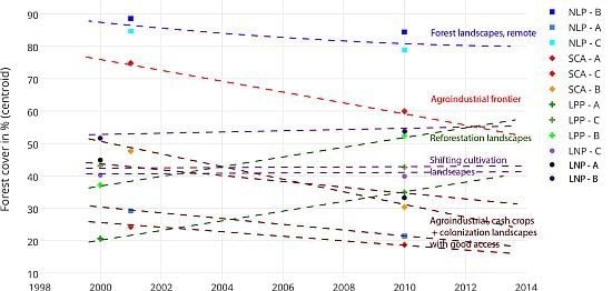
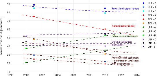
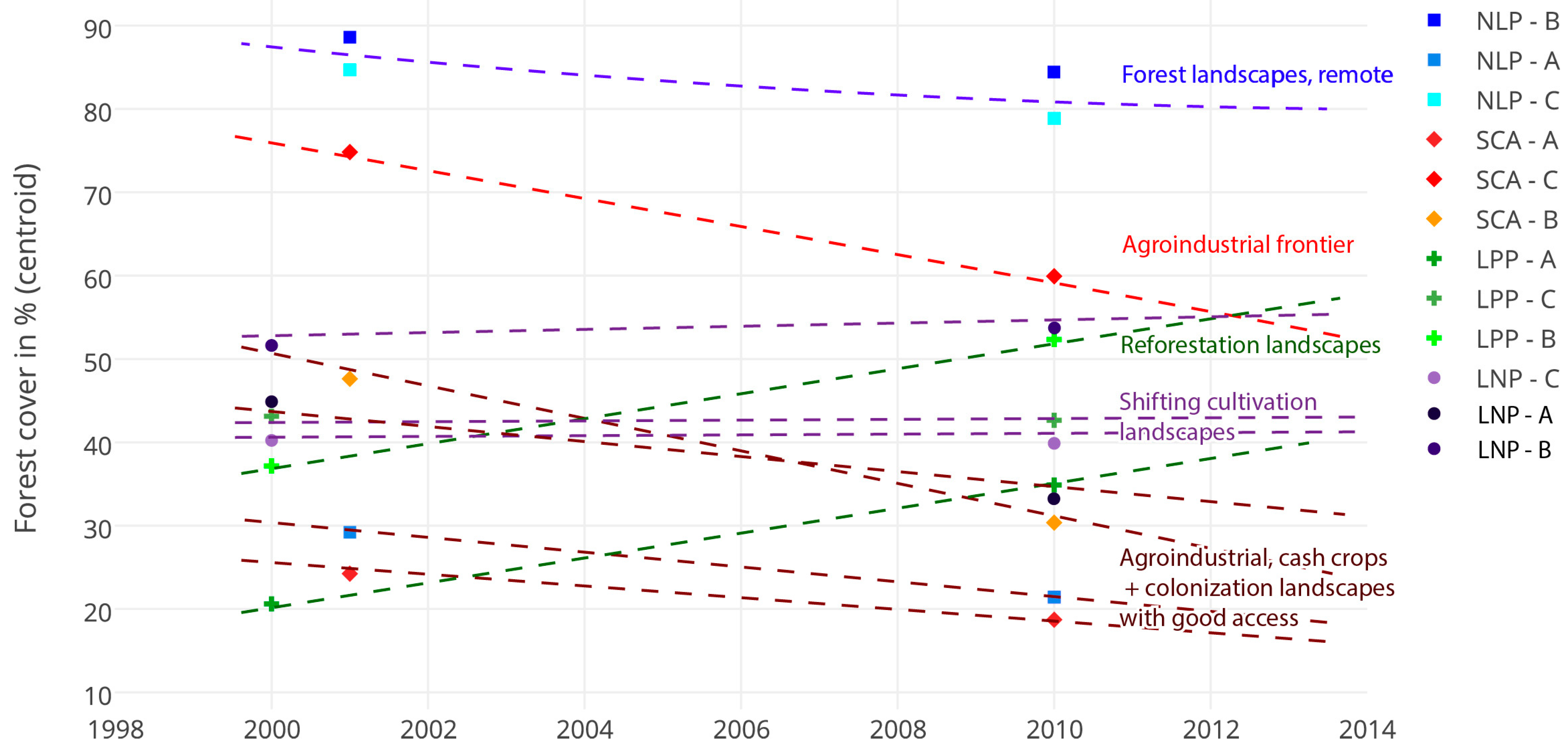
2.5. A Typology of Social Ecological-Contexts and Their Possible Outcomes

Table 10 shows a typology of social-ecological contexts in the four areas, derived from a k-means cluster analysis in three classes per area including socio-economic, cultural and land-use change variables. The quantitative values represent the cluster centroids. Figure 11 shows an ordering of these contexts along forest cover change, and their possible landscape outcomes in the middle-term under a “business as usual” scenario.

Table 10. A typology of social-ecological contexts in the four study areas.

	Population Density (h/km2)	Accessibility (Distance to Road in h)	Poverty (% of Population)	Ethnicity	Forest Cover Change
					Fcover (t0)%	Fcover (t1)%	Rate
North of La Paz Forest Landscape
NLP-A	High	Average	Extreme	Andean	29.2	21.4	−0.09
	20.5	3.5	97.2	86.3%
NLP-B	Average	Remote	Very High	Andean	88.6	85.6	−0.0005
	11.1	5.1	89.9	85.2%
NLP-C	Low	Very remote	Very High	Lowl. 33.6%	84,7	78,9	−0.01
	6.3	7.7	88.1	Non-I. 47.9%
Santa Cruz Agroindustrial Área
SCA-A	High	Very good	High	Non-I. 66.7%	24.2	18.7	−0.02
	21.4	0.7	70.9
SCA-B	Average	Good	Extreme	Andean 65%	47.6	30.4	−0.06
	10.4	1,6	90.8
SCA-C	Average	Average	High	Non-I. 67.2%	74.8	59,9	−0.03
	8.2	3.1	76.9
Luang Prabang Province
LPP-A	High	Average	Average	Tai-K. 31.2%	20.6	34,9	+0.06
	37.9	3.4	40.4	Austr. 50.6%
LPP-B	Average	Remote	High	Austr. 71.2%	37.2	52,3	+0.03
	15.9	4.5	52.4
LPP-C	Average	Very remote	High	Austr. 68.7%	43.1	42,6	−0.01
	10.9	6.15	57.7
Luang Namtha Province
LNP-A	High 35.3	Good 1.5	Average 37.4	Tai-K. 21,5% Austr. 21,6% My.-Tb- 56.1%	44.4	33.2	–0.03
LNP-B	Average 13.5	Average 3.5	Average 48.5	Austr. 36,6% My.-Tb- 53.2%	51.4	52,8	+0.02
LNP-C	High 24.2	Very remote 5.75	Average 47.0	Austr. 42,1% My.-Tb- 44.6%	40.2	39.9	–0.01

Table 10. A typology of social-ecological contexts in the four study areas.

	Population Density (h/km2)	Accessibility (Distance to Road in h)	Poverty (% of Population)	Ethnicity	Forest Cover Change
					Fcover (t0)%	Fcover (t1)%	Rate
North of La Paz Forest Landscape
NLP-A	High	Average	Extreme	Andean	29.2	21.4	−0.09
	20.5	3.5	97.2	86.3%
NLP-B	Average	Remote	Very High	Andean	88.6	85.6	−0.0005
	11.1	5.1	89.9	85.2%
NLP-C	Low	Very remote	Very High	Lowl. 33.6%	84,7	78,9	−0.01
	6.3	7.7	88.1	Non-I. 47.9%
Santa Cruz Agroindustrial Área
SCA-A	High	Very good	High	Non-I. 66.7%	24.2	18.7	−0.02
	21.4	0.7	70.9
SCA-B	Average	Good	Extreme	Andean 65%	47.6	30.4	−0.06
	10.4	1,6	90.8
SCA-C	Average	Average	High	Non-I. 67.2%	74.8	59,9	−0.03
	8.2	3.1	76.9
Luang Prabang Province
LPP-A	High	Average	Average	Tai-K. 31.2%	20.6	34,9	+0.06
	37.9	3.4	40.4	Austr. 50.6%
LPP-B	Average	Remote	High	Austr. 71.2%	37.2	52,3	+0.03
	15.9	4.5	52.4
LPP-C	Average	Very remote	High	Austr. 68.7%	43.1	42,6	−0.01
	10.9	6.15	57.7
Luang Namtha Province
LNP-A	High 35.3	Good 1.5	Average 37.4	Tai-K. 21,5% Austr. 21,6% My.-Tb- 56.1%	44.4	33.2	–0.03
LNP-B	Average 13.5	Average 3.5	Average 48.5	Austr. 36,6% My.-Tb- 53.2%	51.4	52,8	+0.02
LNP-C	High 24.2	Very remote 5.75	Average 47.0	Austr. 42,1% My.-Tb- 44.6%	40.2	39.9	–0.01

Remote contexts in the NLP area (NLP-B and C) have high forest cover and experience little loss; they are inhabited by Andean, lowland indigenous and non-indigenous people. Without specific colonization plans, these areas are likely to keep a high forest cover. A context of rapid forest loss appears however in the SCA area (SCA-C) and corresponds to the agroindustrial frontier, with average remoteness, dominance of non-indigenous peoples, but still with high poverty. Areas with less baseline forest cover, but still with important net losses, have good accessibility and are inhabited by both Andean and non-indigenous people (SCA-A and B), with high extreme poverty in the first case. Landscapes with Andean colonists, forest loss and extreme poverty appear in both NLP and SCA cases (NLP-A and SCA-B). Though some forest gain areas exist in these contexts, loss is likely to dominate and a nearly complete loss of forest can be predicted in the middle term in this topographically uniform, flat landscape. Good accessible contexts with cash crop development in the LNP area (LNP-A) follow a similar path, though the establishment of rubber plantations means that vegetation will increase again, but should not be mistaken as forest regrowth. Rubber expansion is likely to extend to hill areas, similar to neighboring China.

Figure 11. Social-ecological contexts and their possible outcomes in the four study areas.

Figure 11. Social-ecological contexts and their possible outcomes in the four study areas.

Besides the latter case from LNP, two additional types of contexts are visible from the Lao cases: more remote areas, dominated by ethnic minorities, show little net change, which can be interpreted as a balance between forest loss and gain in shifting cultivation landscapes (LPP-C; LNP-B and C), and will probably keep these pathways, or might increase forests with the application of policies aiming at reducing shifting cultivation. Contexts in the LPP areas where forest is increasing (LPP-A and B) also have minority ethnicity, but mixed with ethnic Lao where forest gain rate is higher. These contexts constitute forest regrowth landscapes linked with land planning and resettlement policies, and are likely to reach a top in forest cover concentrated in hills and slopes.

3. Discussion

3.1. What Drives Forest Cover Change in the Study Areas

In the four studied cases, distance to roads and population centers is clearly an important variable which affects forest cover. In three of the four cases, forest loss decreases with distance and the development of infrastructure and market accessibility can be considered a key driver of forest loss. Nevertheless, accessibility must be coupled with economic and policy drivers that foster forest loss: Andean colonization of lowlands and occupancy-based land ownership in Bolivia, soybean expansion in Santa Cruz and rubber plantation expansion in the Luang Namtha province. The exception of Luang Prabang Province where forest gain has occurred in more accessible areas sheds further light into the interaction between accessibility and other land use change drivers. Similar situations have been found in Vietnam, where easily accessible areas, inhabited by ethnically dominant groups, have gained forest [29,83]. The nature and quality of gained forest in Luang Prabang remains unknown, yet documented cases in neighboring Vietnam show that both market integration and policies aiming at reducing shifting cultivation led to agricultural intensification and abandonment of upland agriculture in well-connected villages [83]. With these examples, we can conclude that accessibility is a key driver of forest cover change, yet other underlying causes determine positive or negative forest cover change, and their intensity is felt gradually with increasing population density and accessibility.

Are there differences in forest cover change between landscapes highly connected to international markets, and landscape oriented at subsistence farming or local markets? As stated by Sunderlin et al. [23], there is a gradient of use intensity from hunting-gathering forest dwellers to shifting cultivation and sedentary agriculture, which leads to increased forest loss but at the same time increased extraction of exchange value from the land. In this context, intermediary landscapes such as shifting cultivation areas should experience both forest loss and gain. Such cases were found in more remote areas of Luang Prabang and Luang Namtha as well as more remote Andean settlements in the North of La Paz. As accessibility increases in a context of economic opportunities to convert forest, forest loss increases too. These areas are also clearly impacted by rural migration, as stated by Carr (2009), which in this case is to be related to national policies On the one hand, policies encourage immigration by opening roads, which then becomes spontaneous, like in the North of La Paz area. On the other hand, policies might encourage out-migration like the resettlement and LUPLA policies implemented in Luang Prabang. Both policies are motivated by strategic interests: territorial occupancy and national integration in the case of Bolivia [84], and meeting development goals, drug eradication and national security in the case of Laos [46,81].

Highly connected landscapes would be expected to show high forest loss and insignificant gain. These landscapes are, however, difficult to separate from smallholder landscapes using socio-economic variables. In Luang Namtha, forest gain is indeed lower where ethnic Lao dominate, yet rubber plantation expansion cannot be assigned to this ethnic group only. Forest conversion motivated by transnational markets is also expected to be limited to most productive and rentable lands, and leave marginal lands in forest. Yet the nature of what “marginal” means depends on the commodity which is to be produced. Because a rough terrain is still suitable for rubber and its strategic position, the Luang Namtha area is no more considered marginal and does not follow the forest transition scheme found in Luang Prabang. Will the development of new crops lead big companies to encroach into smallholder’s land? In both Santa Cruz and Luang Namtha, agroindustrial companies coexist with smallholders, and are expected to increasingly encroach into their lands, being able to overcome regulations aimed at protecting them, as observed in Santa Cruz [72,73].

3.2. Poverty, Development and Forest Cover Change

The Bolivian cases show a general trend of increasing forest loss with poverty and extreme poverty, but also with forest gain in these areas, overcoming forest loss only in extremely poor and remote communities. In Laos, poverty is related with reduced forest gain (Luang Prabang) or reduced forest loss (Luang Namtha). However, the multivariate model showed significant relationships between poverty and forest loss only in the North of La Paz, in the remote areas of Luang Prabang, and with gain in both Bolivian cases. Remote areas with both high poverty and forest gain could be observed in the North of La Paz and Luang Namtha, situations that were also found in Vietnam by Vu et al. [29]. We conclude that poverty does not seem to be a driver of deforestation but rather cash crop opportunities coupled with accessibility.

Are communities becoming less poor thanks to economic activities that require deforestation, or richer communities able to invest in commercial crops which provoke deforestation? Poverty reduction through land redistribution is a pillar of the Bolivian colonization policy. Does then, deforestation lead to poverty reduction? Converting natural capital into economic capital has been shown a way of escaping poverty [85], and Bolivia and Laos rank particularity high in natural capital with their high forest cover and low population densities. The case of Luang Namtha, with spontaneous migration from the hills into rubber plantations and the active engagement of villagers in this process might support this hypothesis. However, initial investments can only be made by already wealthy people, since rubber plantations are still at a young stage and are only productive after seven years. In this context, poorer people are likely to be involved as wage laborers but not to establish plantations themselves.

Furthermore, correlation does not mean causality. A correlation between high forest loss and high poverty rate does not mean that the poorer the people, the more they cut forest. As stated above, people able to invest in rubber plantations are not the poorest, thus contradicting this assertion. Does then poverty reduction lead to deforestation? In both cases of Santa Cruz and Luang Namtha, capital investment in cash crops have come from investors from neighboring powerful economies, or from better-off nationals, not from rural people who have been lifted out of poverty. The case of Santa Cruz appears then emblematic: large-scale forest clearing investments are occurring in areas where extreme poverty persists. On the one hand, this highlights a limitation of linking people to observed land parcels and pixels. These land units might not been directly controlled by the people who settle nearby, and inversely, local people might control more remotely located lands. In this sense, there is a trade-off between single-sector analyses, which focus on general causes at a broader scale, and place-bases analyses which miss linkages to the general picture [4]. On the other hand, even if it increased the GDP of a country, this development model leads to highly unequal outcomes, and further marginalizes the weakest social groups, while at the same time having huge environmental impacts. This appears then as a “lose-lose” situation, when both the majority of humans and the environment are disadvantaged [23]. This area would therefore constitute a “land governance hotspot”, where both social and ecological aspects of development face important challenges related to the distribution of both land resources and the impact of their use. The case of Santa Cruz shows some similarities with the Luang Namtha case: presence of local smallholders, cash crop boom driven by investors from powerful neighbor countries, and arrangements able to overcome national protective policies, it might thus be a predictor of what could happen there in the middle term. We must have however some caution in interpreting the situation in Santa Cruz, since poverty data from Bolivia date back 2001, with the country having experienced sustained economic growth and poverty reduction since then.

These considerations allow to give tentative answers to our two first hypotheses: accessibility is an important determinant of forest cover change, yet mediated by economic and policy context. Therefore, no regular pattern from “rich” areas in forest transition and “poor” remote areas could be found. On the other hand, pressures and demands for commodities still drive forest loss in relatively developed areas, such as Santa Cruz, while poorer areas like Luang Prabang are following the forest transition pathway in the absence of such pressures.

3.3. Ethnicity and Typologies of Social-Ecological Systems

As an important characteristic of social-ecological systems, ethnicity was found to be a moderate explanatory of forest cover change. In both Bolivian cases, Andean population proportion correlates with forest loss, but, to a lesser extent, also forest gain, linked with the practice of fallow in settlements. Lowland indigenous peoples are related to less forest loss and more gain, while non-indigenous population has less loss and less gain. In Laos, ethnic groups more related to forest loss vary across cases, being the ethnic Lao in LNP and the Austroasiatic in LPP. Furthermore, ethnic Lao show negative correlations with both forest loss and gain, suggesting more static landscapes than in shifting cultivation areas. Though found to be important variables in one of the first “people-to-pixel” approaches [28], land use practices linked with ethnic groups should not, however, be essentialized. As shown in Northern Laos [53] and in the Bolivian Andes [86], very diverse land use practices can exist within an ethnic group. Cultural aspects should rather be considered as a pool of use options considered acceptable by a group, which are then modeled by socio-economic contexts. In this sense, ethnicity also appears as a cluster of converging socio-economic characteristics inherited by the history of groups that partly determine their location, settlement schemes, and access to land resources and to investment capital. Thus ethnicity appears to be a useful variable to characterize social-ecological systems and build typologies, but only when combined with other socio-economic aspects.

4. Conclusions

We assessed relationships between population density, poverty, ethnicity, accessibility and forest cover change during the 2000s decade for four regions of Bolivia and the Lao PDR. Our findings show that accessibility to roads and population centers is the strongest driver of forest cover change. However, it only makes sense when combined with other underlying economic and policy-related drivers. In three of the four cases, forest loss increased with accessibility in contexts of cash crop expansion and colonization. In the last case (Luang Prabang province in Lao PDR), forest gain increased with accessibility, due to land planning and intensification policies. Our results also show that forest loss does not necessarily concentrate in areas with intermediate poverty and remoteness, since in cash crop expanding landscapes, forest loss still occurs in densely populated areas.

Poverty has weak relationships with forest cover change, but might co-exist with forest loss, while also co-existing with forest gain in very remote areas. Investments are needed to convert forest to other land uses, but these investments can be performed be people who do not reside in the study area, thus making the “people-to-pixels” link more difficult. On the other hand, combination of massive forest loss and high poverty constitute challenging land governance contexts. Coming back to the challenges posed by Rindfuss et al. [1], we can observe that the criterion of aggregating the data at fitting scales was fulfilled, but that the link between land cover change and people determined by residence during censuses and travel time, might mask more external actors that take land use decisions. This is especially true for agroindustrial landscapes, where land use decisions become more and more telecoupled and disconnected from the affected territories [87].

Can census and land cover variables contribute to a diagnostic approach of social-ecological systems? As stated above, some key challenging configurations could be identified, such as market integration, national policy enforcement and unequal landscapes. A challenge is the resolution of land cover datasets, which might poorly capture very small-scale cultivation, as it seems to be the case in the Luang Prabang area, where shifting cultivation might be underestimated by misinterpreting fallows as secondary forest. The space-time match remains acceptable in Laos with census data taken at the middle of the assessed cover change period, but more problematic in Bolivia when census data were only available at the beginning of the study period. Finally, a meso-scale study cannot capture the way local organizations cope with change. Rather, it informs on the possible extent of contexts which should then be further characterized with studies at finer scales.

The methodology used, however, has opened new pathways of understanding forest cover change at middle scales. The recent release of high-resolution data on land cover change [35] might offer promising options to expand the area of study and insert these case studies into the big picture. On the other hand, more data could be incorporated into the analysis, including protected areas, indigenous territories, and land and extractive concessions.

References

1. Rindfuss, R.R.; Walsh, S.J.; Turner, B. L.; Fox, J.; Mishra, V. Developing a science of land change: Challenges and methodological issues. Proc. Natl. Acad. Sci. USA 2004, 101, 13976–13981. [Google Scholar] [CrossRef] [PubMed]
2. Ostrom, E.; Cox, M. Moving beyond panaceas: A multi-tiered diagnostic approach for social-ecological analysis. Environ. Conserv. 2010, 37, 451–463. [Google Scholar] [CrossRef]
3. Messerli, P.; Heinimann, A.; Epprecht, M.; Souksavath, P.; Chanthalanouvong, T.; Minot, N. Socio-Economic Atlas of the Lao PDR—An Analysis Based on the 2005 Population and Housing Census; Swiss National Center of Competence in Research (NCCR) North-South. Geographica Bernensia: Bern, Switzerland/Vientiane, Lao, 2008. [Google Scholar]
4. Turner, B.L.; Lambin, E.F.; Reenberg, A. The emergence of land change science for global environmental change and sustainability. Proc. Natl. Acad. Sci. USA 2007, 104, 20666–220671. [Google Scholar] [CrossRef] [PubMed]
5. Lambin, E.F.; Turner, B.L.; Geist, H.J.; Agbola, S.B.; Angelsen, A.; Bruce, J.W.; Coomes, O.T.; Dirzo, R.; Fischer, G.; Folke, C.; et al. The causes of land-use and land-cover change: Moving beyond the myths. Glob. Environ. Chang. 2001, 11, 261–269. [Google Scholar] [CrossRef]
6. Geist, H.J.; Lambin, E.F. Proximate causes and underlying driving forces of tropical deforestation: Tropical forests are disappearing as the result of many pressures, both local and regional, acting in various combinations in different geographical locations. BioScience 2002, 52, 143–150. [Google Scholar] [CrossRef]
7. Lambin, E.F.; Geist, H.J.; Lepers, E. Dynamics of land-use and land-cover change in tropical regions. Annu. Rev. Environ. Resour. 2003, 28, 205–241. [Google Scholar] [CrossRef]
8. Geist, H.; McConnell, W.; Lambin, E.; Moran, E.; Alves, D.; Rudel, T. Causes and trajectories of land-use/cover change. In Land-Use and Land-Cover Change; Lambin, E., Geist, H., Eds.; Global Change—The IGBP Series; Springer: Berlin Heidelberg, Germany, 2006; pp. 41–70. [Google Scholar]
9. Coomes, O.T.; Grimard, F.; Potvin, C.; Sima, P. The fate of the tropical forest: Carbon or cattle? Ecol. Econ. 2008, 65, 207–212. [Google Scholar] [CrossRef]
10. Berkes, F. Devolution of environment and resources governance: Trends and future. Environ. Conserv. 2010, 37, 489–500. [Google Scholar] [CrossRef]
11. Ostrom, E. A diagnostic approach for going beyond panaceas. Proc. Natl. Acad. Sci. USA 2007, 104, 15181–15187. [Google Scholar] [CrossRef] [PubMed]
12. George, A.; Bennett, A. Case Studies and Theory Development in the Social Sciences; MIT Press: Cambridge, MA, USA, 2005. [Google Scholar]
13. Carr, D. Population and deforestation: Why rural migration matters. Prog. Hum. Geogr. 2009, 33, 355–378. [Google Scholar] [CrossRef] [PubMed]
14. Verburg, P.H.; Overmars, K.P.; Witte, N. Accessibility and land-use patterns at the forest fringe in the northeastern part of the Philippines. Geogr. J. 2004, 170, 238–255. [Google Scholar] [CrossRef]
15. Mather, A.S.; Needle, C.L. The forest transition: A theoretical basis. Area 1998, 30, 117–124. [Google Scholar] [CrossRef]
16. Grau, H.R.; Aide, M. Globalization and land-use transitions in Latin America. Ecol. Soc. 2008, 13, 16. [Google Scholar]
17. Meyfroidt, P.; Lambin, E.F. Global forest transition: Prospects for an end to deforestation. Annu. Rev. Environ. Resour. 2011, 36, 343–371. [Google Scholar] [CrossRef]
18. Mink, S.D. Poverty, Population, and the Environment; World Bank Discussion Papers; The World Bank: Washington, DC, USA, 1993. [Google Scholar]
19. Grossman, G.M.; Krueger, A.B. Economic growth and the environment. Q. J. Econ. 1995, 110, 353–377. [Google Scholar] [CrossRef]
20. Roy Chowdhury, R.; Moran, E.F. Turning the curve: A critical review of Kuznets approaches. Environ. Kuznets Curves Environ. Dev. Res. 2012, 32, 3–11. [Google Scholar]
21. Kauppi, P.E.; Ausubel, J.H.; Fang, J.; Mather, A.S.; Sedjo, R.A.; Waggoner, P.E. Returning forests analyzed with the forest identity. Proc. Natl. Acad. Sci. USA 2006, 103, 17574–17579. [Google Scholar] [CrossRef] [PubMed]
22. Wunder, S. Poverty alleviation and tropical forests—What scope for synergies? World Dev. 2001, 29, 1817–1833. [Google Scholar] [CrossRef]
23. Sunderlin, W.D.; Angelsen, A.; Belcher, B.; Burgers, P.; Nasi, R.; Santoso, L.; Wunder, S. Livelihoods, forests, and conservation in developing countries: An overview. Livelihoods For. Conserv. 2005, 33, 1383–1402. [Google Scholar]
24. Suri, V.; Chapman, D. Economic growth, trade and energy: Implications for the environmental Kuznets curve. Ecol. Econ. 1998, 25, 195–208. [Google Scholar] [CrossRef]
25. Robbins, P. Political Ecology, 2nd ed.; John Wiley and Sons: Chichester, UK, 2009. [Google Scholar]
26. Gerber, J.-F. Conflicts over industrial tree plantations in the South: Who, how and why? Glob. Environ. Chang. 2011, 21, 165–176. [Google Scholar] [CrossRef]
27. Epprecht, M.; Müller, D.; Minot, N. How remote are Vietnam’s ethnic minorities? An analysis of spatial patterns of poverty and inequality. Ann. Reg. Sci. 2011, 46, 349–368. [Google Scholar] [CrossRef]
28. Lambin, E. L’Apport de la teledetection dans l’etude des systemes agraires d’Afrique: l’exemple du Burkina Faso. Africa 1988, 58, 337–352. [Google Scholar] [CrossRef]
29. Chi, V.; van Rompaey, A.; Govers, G.; Vanacker, V.; Schmook, B.; Hieu, N. Land transitions in Northwest Vietnam: An Integrated analysis of biophysical and socio-cultural factors. Hum. Ecol. 2013, 41, 37–50. [Google Scholar] [CrossRef]
30. Collier, P. The Bottom Billion Why the Poorest Countries are Failing and What Can Be Done about It; Oxford University Press: Oxford, UK, 2007. [Google Scholar]
31. United Nations Conference on Trade and Development (UNCTAD). Review of Maritime Transport; United Nations: New York & Geneva, NY, USA/Switzerland, 2010. [Google Scholar]
32. Lewis, P. Ethnologue: Languages of the World, 6th ed.; SIL International: Dallas, TX, USA, 2009. [Google Scholar]
33. Costanza, R.; dʼArge, R.; de Groot, R.; Farber, S.; Grasso, M.; Hannon, B.; Limburg, K.; Naeem, S.; OʼNeill, R.V.; Paruelo, J.; et al. The value of the world’s ecosystem services and natural capital. Nature 1997, 387, 253–260. [Google Scholar] [CrossRef]
34. Food and Agriculture Organization of the United Nations (FAO). State of the World’s Forests; FAO: Rome, Italy, 2011. [Google Scholar]
35. Hansen, M.C.; Potapov, P.V.; Moore, R.; Hancher, M.; Turubanova, S.A.; Tyukavina, A.; Thau, D.; Stehman, S.V.; Goetz, S.J.; Loveland, T.R.; et al. High-resolution global maps of 21st-century forest cover change. Science 2013, 342, 850–853. [Google Scholar] [CrossRef] [PubMed]
36. Killeen, T.J.; Guerra, A.; Calzada, M.; Correa, L.; Calderon, V.; Soria, L.; Quezada, B.; Steiniger, M.K. Total historical land-use change in eastern Bolivia: Who, where, when, and how much? Ecol. Soc. 2008, 13, 36. [Google Scholar]
37. Pacheco, P. Agricultural expansion and deforestation in lowland Bolivia: The import substitution versus the structural adjustment model. Land Use Policy 2006, 23, 205–225. [Google Scholar] [CrossRef]
38. Lerch, L. The geopolitics of land: Population, security and territory viewed from the international financing of the land survey in Bolivia (1996–2013). J. Lat. Am. Geogr. 2014, 13, 137–168. [Google Scholar] [CrossRef]
39. Redo, D.; Millington, A. C.; Hindery, D. Deforestation dynamics and policy changes in Bolivia’s post-neoliberal era. Land Use Policy 2011, 28, 227–241. [Google Scholar] [CrossRef]
40. Bottazzi, P.; Dao, H. On the road through the Bolivian Amazon: A multi-level land governance analysis of deforestation. Land Use Policy 2013, 30, 137–146. [Google Scholar] [CrossRef]
41. Instituto Nacional de Estadistica y Censos. VI Censo Nacional de Población y Vivienda 2001; Republica del Ecuador, Instituto Nacional de Estadistica y Censos: San José, Costa Rica, 2001. [Google Scholar]
42. Anthias, P.; Radcliffe, S.A. The ethno-environmental fix and its limits: Indigenous land titling and the production of not-quite-neoliberal natures in Bolivia. Geoforum 2013. [Google Scholar] [CrossRef]
43. Pacheco, P.; Mertens, B. Land use change and agriculture development in Santa Cruz, Bolivia. Bois Forets Trop. 2004, 280, 29–40. [Google Scholar]
44. Steininger, M.K.; Tucker, C.J.; Ersts, P.; Killeen, T.J.; Villegas, Z.; Hecht, S.B. Clearance and fragmentation of tropical deciduous forest in the Tierras Bajas, Santa Cruz, Bolivia. Conserv. Biol. 2001, 15, 856–866. [Google Scholar] [CrossRef]
45. Ducourtieux, O.; Laffort, J.-R.; Sacklokham, S. Land policy and farming practices in Laos. Dev. Chang. 2005, 36, 499–526. [Google Scholar] [CrossRef]
46. Lestrelin, G. Land degradation in the Lao PDR: Discourses and policy. For. Transit. Wind Power Plan. Landsc. Publics 2010, 27, 424–439. [Google Scholar]
47. Lestrelin, G.; Bourgoin, J.; Bouahom, B.; Castella, J.-C. Measuring participation: Case studies on village land use planning in northern Lao PDR. Appl. Geogr. 2011, 31, 950–958. [Google Scholar] [CrossRef]
48. Evrard, O.; Goudineau, Y. Planned resettlement, unexpected migrations and cultural trauma in Laos. Dev. Chang. 2004, 35, 937–962. [Google Scholar] [CrossRef]
49. Schönweger, O.; Heinimann, A.; Epprecht, M.; Lu, J.; Thalongsengchanh, P. Concessions and Leases in the Lao PDR. Taking Stock of Land Investments; Geographica Bernensia, Centre for Development and Environment (CDE), University of Bern: Bern, Switzerland/Vientiane, Lao, 2012. [Google Scholar]
50. Condominas, G. Anthropological reflections on swidden change in Southeast Asia. Hum. Ecol. 2009, 37, 265–267. [Google Scholar] [CrossRef]
51. Zuckerman, C. Lao Lum, Lao Theung, Lao Suung. A Few Reflections on Somme Common Lao Ethnonyms. Available online: http://seap.einaudi.cornell.edu/system/files/Lao%20Lum,%20Lao%20Theung,%20Lao%20Suung%20%28Author%20%20Charles%20Zuckerman%29.pdf (accessed on 15 March 2014).
52. Chazée, L. The Peoples of Laos. Rural and Ethnic Diversities; White Lotus: Bangkok, Thailand, 2002. [Google Scholar]
53. Ducourtieux, O. Du riz et des arbres. L’interdiction de L’agriculture D’abattis-brûlis, une constante politique au Laos; IRD-Karthala: Paris, France, 2009. [Google Scholar]
54. Heinimann, A.; Hett, C.; Hurni, K.; Messerli, P.; Epprecht, M.; Jørgensen, L.; Breu, T. Socio-economic perspectives on shifting cultivation landscapes in northern Laos. Hum. Ecol. 2013, 41, 51–62. [Google Scholar] [CrossRef] [Green Version]
55. Stich, C. Dynamics of Resettlement, Land Tenure, Water Resource Use and Irrigation Governance in Nam Khan Watershed, Lao PDR. Master’s Thesis, Université de Genève, Geneva, Switzerland, 2013. [Google Scholar]
56. Thongmanivong, S.; Fujita, Y.; Fox, J. Resource use dynamics and land-cover change in Ang Nhai Village and Phou Phanang National Reserve forest, Lao PDR. Environ. Manag. 2005, 36, 382–393. [Google Scholar] [CrossRef]
57. Guntern, M. Etude multi-scalaire des mutations territoriales du Nord-Laos. Les répercussions engendrées par les plantations d’hévéas sur les moyens de subsistance et l’industrie touristique dans le District de Luang Namtha. Master’s Thesis, Université de Genève, Geneva, Switzerland, 2013. [Google Scholar]
58. Molina, R.; Albó, X. Gama étnica Y lingüística de la población Boliviana; Sistema de las Naciones Unidas en Bolivia: La Paz, Bolivia, 2006. [Google Scholar]
59. Diez Astete, A. Compendio de etnias indígenas y ecoregiones. Amazonia, Oriente y Chaco; Centro de Servicios Agropecuarios y Socio-Comunitarios; Plural Editores: La Paz, Bolivia, 2011. [Google Scholar]
60. Feres, J.C.; Mancero, X. El Método de las necesidades BáSICAS insatisfechas (NBI) y sus aplicaciones en América Latina; Cepal/Naciones Unidas: Santiago, Chile, 2001. [Google Scholar]
61. Instituto Nacional de Estadística. Cálculo del Indicador de Necesidades Básicas Insatisfechas en Bolivia; Instituto Nacional de Estadística: La Paz, Bolivia, 2004. [Google Scholar]
62. Frakes, B.; Hurst, C.; Pillmore, D.; Schweiger, B.; Talbert, C. Travel Time Cost Surface Model, Version 1.7; Rocky Mountain Network-National Park Service: Fort Collins, CO, USA, 2008. [Google Scholar]
63. Messerli, P.; Heinimann, A.; Epprecht, M. Finding homogeneity in heterogeneity—A new approach to quantifying landscape mosaics developed for the Lao PDR. Hum. Ecol. 2009, 37, 291–304. [Google Scholar] [CrossRef] [Green Version]
64. Lao Statistics Bureau, Ministry of Natural Resources and Environment, Ministry of Agriculture and Forestry. Lao DECIDE Info. Available online: http://www.decide.la (accessed on 30 July 2013).
65. Sahr, K.; White, D.; Kimerling, A.J. Geodesic discrete global grid systems. Cartogr. Geogr. Inf. Sci. 2003, 30, 121–134. [Google Scholar] [CrossRef]
66. Puyravaud, J.-P. Standardizing the calculation of the annual rate of deforestation. For. Ecol. Manag. 2003, 177, 593–596. [Google Scholar] [CrossRef]
67. Aguiar, A.P.D.; Câmara, G.; Escada, M.I.S. Spatial statistical analysis of land-use determinants in the Brazilian Amazonia: Exploring intra-regional heterogeneity. Ecol. Model. 2007, 209, 169–188. [Google Scholar] [CrossRef]
68. Farfán, W. Venta de coca producida en Apolo carece de control. La Razón. 2013. Available online: http://www.la-razon.com/index.php?_url=/seguridad_nacional/Venta-producida-Apolo-carece-control_0_1931806892.html (accessed on 20 February 2014).
69. Forrest, J.L.; Sanderson, E.W.; Wallace, R.; Lazzo, T.M.S.; Cerveró, L.H.G.; Coppolillo, P. Patterns of land cover change in and around Madidi National Park, Bolivia. Biotropica 2008, 40, 285–294. [Google Scholar] [CrossRef]
70. Sandoval, Y. Gestión territorial en áreas indígenas Tierra Comunitaria de Origen Tacana, Bolivia; Universidad de Zaragosa: Zaragosa, Spain, 2013. [Google Scholar]
71. Locklin, C.C.; Haack, B. Roadside measurements of deforestation in the Amazon Area of Bolivia. Environ. Manag. 2003, 31, 774–783. [Google Scholar] [CrossRef]
72. Urioste, M. Concentración y extranjerización de la tierra en Bolivia; Fundación Tierra: La Paz, Bolivia, 2011. [Google Scholar]
73. Colque, G. Expansión de la frontera agrícola. Luchas por el control y la apropiación de la Tierra en el oriente Boliviano; Fundación Tierra: La Paz, Bolivia, 2014. [Google Scholar]
74. Pinto-Ledezma, J.N.; Ruiz de Centurion, T. Deforestation and fragmentation patterns 1976–2006 in San Julian district (Santa Cruz, Bolivia). Ecol. Boliv. 2010, 45, 101–115. [Google Scholar]
75. Mertz, O.; Padoch, C.; Fox, J.; Cramb, R.A.; Leisz, S.; Lam, N.; Vien, T. Swidden change in Southeast Asia: Understanding causes and consequences. Hum. Ecol. 2009, 37, 259–264. [Google Scholar] [CrossRef]
76. Hurni, K.; Hett, C.; Heinimann, A.; Messerli, P.; Wiesmann, U. Dynamics of shifting cultivation landscapes in Northern Lao PDR between 2000 and 2009 based on an analysis of MODIS time series and Landsat images. Hum. Ecol. 2013, 41, 21–36. [Google Scholar] [CrossRef]
77. Thongmanivong, S.; Fujita, Y. Recent land use and livelihood transitions in northern Laos. Mt. Res. Dev. 2006, 26, 237–244. [Google Scholar] [CrossRef]
78. Yokoyama, S. Forest, ethnicity and settlement in the mountainous area of northern Laos. Southeast. Asian Stud. 2004, 42, 132–156. [Google Scholar]
79. Lestrelin, G.; Giordano, M. Upland development policy, livelihood change and land degradation: interactions from a Laotian village. Land Degrad. Dev. 2007, 18, 55–76. [Google Scholar] [CrossRef]
80. Shi, W. Rubber Boom in Luand Namtha A Transnational Perspective; GTZ RDMA: Vientiane, Laos, 2008. [Google Scholar]
81. Cohen, P.T. The post-opium scenario and rubber in northern Laos: Alternative Western and Chinese models of development. Int. J. Drug Policy 2009, 20, 424–430. [Google Scholar] [CrossRef] [PubMed]
82. Thongmanivong, S.; Fujita, Y.; Phanvilay, K.; Vongvisouk, T. Agrarian land use transformations in Northern Laos: From swidden to rubber. Southeast Asian Stud. 2009, 47, 330–347. [Google Scholar]
83. Trincsi, K.; Pham, T.-T.-H.; Turner, S. Mapping mountain diversity: Ethnic minorities and land use land cover change in Vietnam’s borderlands. Land Use Policy 2014, 41, 484–497. [Google Scholar] [CrossRef]
84. Garcia Linera, A. Geopolítica de la Amazonia; Vicepresidencia del Estado Plurinacional de Bolivia: La Paz, Bolivia, 2012. [Google Scholar]
85. Vosti, S.A.; Braz, E.M.; Carpentier, C.L.; d’ Oliveira, M. V.; Witcover, J. Rights to forest Products, deforestation and smallholder income: Evidence from the western Brazilian Amazon. Part Spec. Issue Links Poverty Environ. Degrad. Lat. Am. 2003, 31, 1889–1901. [Google Scholar]
86. Boillat, S.; Mathez-Stiefel, S.; Rist, S. Linking local knowledge, conservation practices and ecosystem diversity: Comparing two communities in the Tunari National Park (Bolivia). Ethnobiol. Conserv. 2013, 2, 8. [Google Scholar]
87. Eakin, H.; DeFries, R.; Kerr, S.; Lambin, E.; Liu, J.; Marcotullio, P.J.; Messerli, P.; Reenberg, A.; Rueda, X.; Swaffield, S.R.; et al. Significance of telecoupling for exploration of land-use change. In Rethinking Global Land Use in an Urban Era; MIT Press: Cambridge, UK, 2014; pp. 141–162. [Google Scholar]