Model-Based Synthesis of Locally Contingent Responses to Global Market Signals

Magliocca, Nicholas R.

doi:10.3390/land4030807

Open AccessArticle

Model-Based Synthesis of Locally Contingent Responses to Global Market Signals

by

Nicholas R. Magliocca

National Socio-Environmental Synthesis Center (SESYNC), University of Maryland, 1 Park Place, Annapolis, MD 21409, USA

Land 2015, 4(3), 807-841; https://0-doi-org.brum.beds.ac.uk/10.3390/land4030807

Submission received: 2 July 2015 / Revised: 2 September 2015 / Accepted: 7 September 2015 / Published: 16 September 2015

(This article belongs to the Special Issue Economic Globalization, Telecoupling and Land Change)

Download

Browse Figures

Versions Notes

Abstract

:

Rural livelihoods and the land systems on which they depend are increasingly influenced by distant markets through economic globalization. Place-based analyses of land and livelihood system sustainability must then consider both proximate and distant influences on local decision-making. Thus, advancing land change theory in the context of economic globalization calls for a systematic understanding of the general processes as well as local contingencies shaping local responses to global signals. Synthesis of insights from place-based case studies is a path forward for developing such systematic knowledge. This paper introduces a generalized agent-based modeling framework for model-based synthesis to investigate the relative importance of structural versus agent-level factors in driving land-use and livelihood responses to changing global market signals. Six case-study sites that differed in environmental conditions, market access and influence, and livelihood settings were analyzed. Stronger market signals generally led to intensification and/or expansion of agriculture or increased non-farm labor, while changes in agents’ risk attitudes prompted heterogeneous local responses to global market signals. These results demonstrate model-based synthesis as a promising approach to overcome many of the challenges of current synthesis methods in land change science and identify generalized as well as locally contingent responses to global market signals.

Keywords:

agent-based synthesis system; meta-analysis; effect size; livelihoods; land-use change

Graphical Abstract

1. Introduction

Consumption and production of land-based food, fiber, and fuel are increasingly separated in space through economic globalization [1,2,3]. As a result, understanding place-based land and livelihood change requires an open system approach that considers land-use and livelihood decision-making as a consequence of both local context and broader-scale influences [4]. Further, interactions between local context and broad-scale influences play-out in a myriad of ways resulting in significant land use and/or livelihood transitions in some cases while not in others. Thus, advancing land systems theory within the context of economic globalization calls for a systematic understanding of the general processes as well as local contingencies underlying heterogeneous responses to global signals [4,5,6]. Synthesis of insights from place-based case studies of land and livelihood change is a path forward for developing such systematic knowledge. This paper introduces a model-based synthesis approach to investigating the influence of local socio-environmental and agent-level factors in mediating land-use and livelihood responses to changing global market signals.

Currently, the land change science community recognizes the need to advance theoretical and analytical frameworks that are capable of dealing with both global system-level drivers, or so-called “teleconnections”, of local land-use and livelihood changes [1,7], and also scaling-up local-level processes, such as changing livelihood strategies, to scales relevant to regional and national policy-making [5,8,9]. Similarly, the need to incorporate more realistic representations of land-use change processes, particularly agent-level decision-making, into integrated assessment models and ultimately Earth system models is clear [10]. This requires knowledge of the broad-scale patterns in the causes and consequences of land change as well as the local contingencies within those broad-scale patterns that lead to different local trajectories in response to the same global forcing. Thus, a systematic understanding of the relative importance of structural (i.e., top-down, local land and/or global economic system influences) versus agent-level factors in driving observed land-use and livelihood changes across varied locations and contexts is the ultimate goal for land change theory and prediction in the context of global economic and environmental change [1,7].

Synthesis of local land change observations (i.e., case studies) through methods such as meta-analysis has built systematic knowledge of the causes and consequences of land change across many locations and for many different land change processes (e.g., [11,12,13,14]). Yet, synthesis in land change science faces unique challenges related to the multiple and mixed data types, theoretical lens, and scales of analysis, which all create comparability issues. These comparability issues have constrained explanations of land change produced through synthesis methods to correlative relationships with less statistical rigor/power than meta-analytic methods used in other fields (e.g., meta-analysis of effect sizes [15,16]). Standardized experimental and analytical frameworks are needed to improve the statistical rigor of synthesis research of land change processes [15].

Here, I introduce a model-based synthesis approach that addresses these comparability issues and also leverages the process-level explanatory power of agent-based models (ABMs)—an agent-based synthesis system (ABSS). The ABSS approach retains the primary strength of ABMs—the ability to model micro-level decision-making processes—while using a modeling architecture explicitly designed for large-scale, systematic deployment and synthesis of insights from many site-based ABM simulations. The ABSS approach is an in silico analog to the rigorous synthesis method of a meta-analysis of effect sizes. The work presented here applies a single generalized model structure to six cases taken from three case studies to explore similarities across and local contingencies within land-use and livelihood decision-making in response to changing global market forces. The six test cases come from three different continents and span a wide range of biophysical settings and influence from regional and global markets. Differences in modeled responses to experimental manipulations across the test cases will provide insights into the relative importance of structural versus agent-level factors and processes in driving land use and livelihood outcomes in each context.

In the following section, I describe current concepts for investigating global market drivers of land use and livelihood change, and articulate the conceptual framework that is used here to explore the relative importance of structural and agent-level factors. A brief overview of synthesis methods in land change science is then provided to situate the ABSS approach within the larger family of synthesis methods relevant for land change. The specific characteristics and contexts of the selected case studies are then be provided, and followed by description of the generalized modeling framework and experimental design of the ABSS approach. Simulated land use and livelihood outcomes are then presented and discussed. Finally, I conclude with a discussion of the limitations of and potential for the ABSS approach to provide synthetic, systematic knowledge and advance land change modeling and theory.

2. Background

2.1. Conceptual Framework

Conceptual approaches for investigating local land use and livelihood change in the context of increasing economic globalization vary widely owing to the diversity of disciplines that contribute to land change science. Here, I present a conceptual framework that synthesizes a selection of somewhat disparate but complementary approaches for investigating the local consequences of economic globalization through local-global production and consumption linkages. Specifically I analyze the effects of such local-global linkages on local land use and livelihood decisions through two main points of entry: structural and agency-based explanations. These two perspectives originate from different disciplinary traditions and generally emphasize top-down or bottom-up explanations of local-global linkages, respectively. Although this is presented as a structure-agency dichotomy, this is not meant to imply these explanations stand in isolation, rather the structure-agency distinction serves to highlight different points of entry within a land systems context for analysis. In reality, the approaches discussed below are aligned along a spectrum and, taken together, provide a more comprehensive conceptual framework to investigate local land and livelihood contingencies in response to global conditions than either approach can provide alone.

Structural explanations are rooted in global systems approaches, which are based on the premise that global market production demands on and opportunities for a given location depend the location’s role in global supply chains [17]. Connections to the global economic network can transform local livelihood strategies and the natural landscape through land-use change [2,3,18]. These transformations are an embodiment of conceptions teleconnections and/or “telecoupling” in which production and consumption activities are separated over distance but connected by flows in goods, capital, and/or information [2,19]. The teleconnection concept has been used to study the virtual trade of natural resources such as water [20], embodied human appropriation of net primary production [21,22], and agricultural trade relationships and the displacement of land use [2,17,23]. Teleconnections have also been used to contextualize research on large-scale land acquisitions and natural resources in developing countries by outside investors (e.g., [24,25]). The concept of telecoupling is an extension of teleconnections through the lens of coupled human and natural systems, and tends to be used to investigate a smaller set of interacting entities to understand multi-scale relationships and feedbacks in natural resource use. Telecoupling is defined as “socioeconomic and environmental interactions between coupled human and natural systems over distances” ([1]; p. 27), or a situation in which a disturbance to one system creates a reaction in the flows and processes linking it to other distantly connected systems [7]. Both tele-concepts provide the conceptual frameworks for linking distant global market demand signals to rural production and consequent natural landscape modification through land use decisions. Importantly, however, this paper does not consider the explicit feedbacks between specific locations. Rather, it investigates the one-way effects of global to local market signals, such as those that might be transmitted through teleconnections, on local livelihood and land-use decisions.

The degree to which global market signals, specifically commodity prices, are transmitted directly to local producers is at the heart of the challenge to understand local responses to changing global economic forces. Empirical work by de Janvry et al. [26] showed that the degree of market participation among rural producers is driven by structural features of local markets, namely the relative differences between farmgate crop prices, food prices, and internal cost of production (i.e., “shadow price”). For example, smallholding producers are often observed to allocate labor to producing both for the market and to meet subsistence needs [27,28] due to a perceived “price gap” in which it is profitable to sell crops yet too costly to buy food. This results in market participation rates that may differ from what would be expected given a location’s role in a global commodity chain [26].

The tele-concepts provide structural explanations of the influences of global economic system on specific locations that can be operationalized for empirical analysis using available trade network and flow data, and have produced comprehensive descriptions of the globalized natural resource use. Similarly, the concept of price gaps supports the translation of global market signals to local market realities. However, such approaches have been criticized for being too coarse (e.g., national-scale) and omitting fine-grained sources of heterogeneity that may lead to outcomes different than those predicted at the aggregate level [6,10]. The macro-scale, tele-concepts have been additionally criticized for essentially treating space as a homogeneous container into and out of which flows are calculated with little consideration for how those flows are consumed, produced, and modified within the container [5]. It still remains a challenge to operationalize structural approaches in such a way that heterogeneity in adaptive responses to global market signals can be fully considered.

Alternatively, agency-based explanations of local land and livelihood change in response to global markets are more focused on decision-making factors and their heterogeneity among individuals or households. Price gaps, for instance, emphasize the structural constraints local markets impose on productions decisions, but de Janvry et al. [26] also acknowledge that the shadow price of production can be quite heterogeneous across producers for a number of reasons. The importance of such heterogeneity has also been noted within the sustainable livelihoods and international development literatures to quantify and link agent-level heterogeneity to different levels of market participation. The livelihood assets framework considers multiple forms of household capital (natural, human, social, physical and financial) that vary among households according to social relations, institutions, and natural resource endowments. Linkages are then made between the configuration of assets and production behavior of a given household (e.g., [27,29,30,31,32]). Adaptive responses of households to market signals are further complicated by differences in perception of risks in market participation and on-farm income generating activities. Price shocks, market trends, and climate variability are all potential sources of risk in agricultural production, and rural producers have developed risk-reducing strategies, such as the diversification of income-generating activities, that may lead to production decisions that diverge from purely profit-maximizing behavior [27,28,30,32,33]. Agent-level differences in both risk perception and capability to mobilize assets results in heterogeneous responses to the same global market signals.

Although such approaches account for agent heterogeneity conceptually, empirical analyses often revert to aggregate-level explanations due to the costs of acquiring disaggregated household-level data—a problem that is compounded when conducting comparative research across multiple locations. For example, Winters et al. [30] conducted a meta-analysis of rural livelihood strategies using the rural income-generating activities (RIGA) database. Even though the RIGA database contains multinational household- and village-level survey data, comparative analysis was performed at the national-level, which limited the analysis to correlative relationships unable to link localized adaptive responses to global market forces [34]. Further, livelihoods analyses tend to treat global market signals as exogenous, monolithic factors without consideration of the myriad of ways observed globally that global market structures impose local constraints or opportunities. Thus, it remains difficult to produce agency-based explanations of local land and livelihood change in response to global markets in a cross-site comparative framework.

Structural and agency approaches have generally existed perpendicular to one another even though elements of each are considered by the other. Global economic system approaches often provide a starting point to explain global market influences on local production [35,36]. However, because of the social, institutional, cultural, and knowledge investments in land-use practices, these practices are often central to human identities and can be slow to change, limiting the applicability of strictly market-based explanations [37,38]. Borrowing insights from the field of economic geography, structural constraints imposed on or opportunities available to local producers through global economic systems are interpreted through the social processes and individual heterogeneity that influence land use and livelihood decision-making [5]. Thus, adaptive responses to changing global economic conditions should be understood as the products of interactions between structural market and agent-level characteristics. Conceptually, this synergy is clear, however, there is not an obvious way forward for implementing such an integrated framework—particularly for cross-site, synthesis research—with current analytical approaches. With the explicit representation of land use and livelihood decision processes, the ABSS approach has the analytical framework to provide insights into such questions.

2.2. Synthesis Approaches in Land Change Science

With the relevant conceptual perspectives outlined, attention is now shifted to current approaches to synthesis in land change science to build systematic knowledge of local adaptive responses to global economic changes. Synthesis is a research approach that draws upon and distills many sources of data, ideas, explanations, and methods in order to accelerate knowledge production beyond that of less integrative approaches (see “synthesis” at http://sesync.org/glossary/). In land change science, meta-studies are a sub-group of synthesis methods that are distinct from literature reviews, analytical review methods, and fully quantitative synthesis methods because they (a) conduct analyses across prior case studies of a common phenomenon as the observational unit [39], and (b) possess systematic case selection criteria intended to produce a comprehensive and comparable collection of cases (see [15] for details). Meta-studies of land system change vary from fully quantitative statistical analyses (e.g., [12,16]) to qualitative coding methods such as qualitative comparative analysis (e.g., [13]). Meta-studies in land change science also differ from more rigorous meta-analytic methods, such as meta-analysis of effects sizes, which utilize standardized measurements across cases, explicit “control” and “treatment” groups of observations, and normalized indicators of variance across cases that can be tested for statistical differences [15].

Regardless of the synthesis method, the ability to make systematic comparisons is ultimately limited by the consistency of the methods, documentation, and various theoretical lenses used to conduct the case studies from which the synthesis draws. No standard case-study methodology exists in land change science, which leaves the interpretation and coding of drivers of land system change open to the meta-analyst [39]. Even when such synthesis methods successfully identify common patterns across empirical case studies, they cannot provide mechanistic explanations of how such empirical patterns emerge from underlying processes, and thus lack the means to test hypotheses about sources of contingent local responses to changing global market forces across different contexts. Rindfuss and colleagues [40] have proposed that ABMs, due to their explicit representation of human decision-making, can provide a formal means to synthesize general insights and build theory about the mechanisms driving human-environmental interactions and SES sustainability. However, synthesis across case-based ABMs has been difficult because of inconsistencies in how the same processes/structures are represented across models [41,42]. A synthesis approach is needed that can harness the process-level explanatory ability of ABMs while also eliminating the comparative issues that plague land change science.

3. Experimental Section

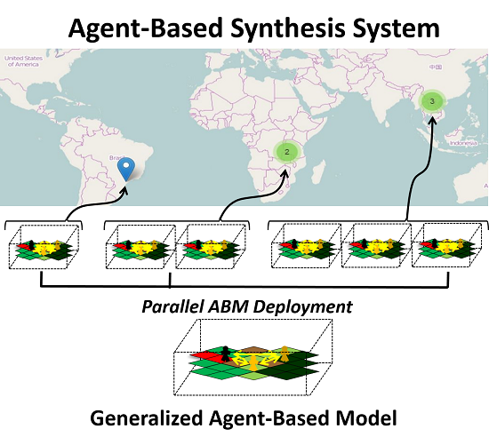
3.1. The Agent-Based Synthesis System Approach

The ABSS approach uses a single generalized model structure as a standardized observational and experimental tool which can be applied across many sites (i.e., “test cases”; see [8]) while maintaining comparability. This approach proceeds through three phases: contextualization, evaluation, and experimentation. In the first phase, each test case must be quantitatively contextualized within the larger analytical extent about which synthesis will make inferences. In this case, the analytical extent is global, and contextualization is done by parameterizing site-specific conditions (e.g., land suitability for agriculture, population density, access to markets) based on the variability (i.e., variable distribution) of such conditions observed globally as described by relevant global datasets (i.e., distribution of variable values observed globally). To ensure wide applicability and comparability, global datasets derived from remote sensing products, statistical models, or other systematic data analysis/collection methods (e.g., agricultural censuses) are used. However, since no comprehensive data exists to explicitly link global market conditions to factors that influence local livelihood and land-use decisions, a set of hypothesized cost and price functions are used to describe local market conditions as a function of global economic settings. The cost and price functions link global market access and influence index values [43] to local farm-gate and food prices, farm input costs, and non-farm wages and transaction costs. Global commodity prices and the U.S. minimum wage represent agricultural commodity prices and non-farm wages realized by a farmer in locations with high market access and a market influence index at or near 1. Local economic factors then diverge from these values according to the cost functions in locations with global market access and influence values less than 1 (see [44] for full description). Biophysical and demographic conditions are taken directly from global geospatial datasets for each test case’s location. Combined, these steps specify the global context in which land-use and livelihood decisions are modeled.

In the evaluation phase, the pattern-oriented modeling (POM; [45]) approach is used to parameterize the general model to ensure a simplified but realistic representation of each test case. POM is a hybrid model evaluation technique appropriate for process-based models because it considers process and outcome accuracy simultaneously [44,45,46]. According to the POM approach, the extent to which a model can simultaneously reproduce multiple target patterns at different system organizational levels—rather than single patterns, such as land use patterns (spatial or non-spatial)—is a reflection of the realism of the model structure, which sets a relatively high bar for structural validation [45,46,47]. Evaluation of structural realism is a particular strength of the POM approach. By evaluating model outcomes based on both primary and secondary target patterns (i.e., patterns that can and cannot be predicted directly from data, e.g., land use versus variability of household consumption, respectively), one can determine both how realistically a processes is represented (e.g., crop production at or above/below subsistence needs (i.e., surplus)) and whether it interacts realistically with other processes to produce similar outcomes to those observed in the real-world (e.g., crop production decisions interact with land use choices to produce particular land use patterns and dynamics).

Target patterns are used in conjunction with machine learning techniques (e.g., genetic algorithm) as performance criteria to identify combinations of free model parameters that produce model outcomes that match all target patterns simultaneously within specified tolerance levels. Free parameters include inputs into the cost and price function parameters, as well as other structural parameters controlling site-specific spatial factors of land-use decisions (e.g., average farm size). Once a suite of parameter combinations is identified that produces model outcomes that match all target patterns, one can have confidence that the parameterized model is capable of satisfactory levels of structural and outcome accuracy [44,47]. Specific model evaluation criteria are discussed in detail later in the paper.

Finally, the parameterized general model is experimentally manipulated to compare heterogeneous agent-level responses across test cases. Following the methodology of meta-analysis of effect sizes, successful model runs from the evaluation phases (i.e., parameterizations that reproduced target patterns) are considered the baseline, or “control”, and subsequent simulations with experimental settings as “treatments”. The specific local and contextual conditions in which each test case is embedded (e.g., local climate, access to markets, household labor supply, etc.) interact with experimental treatments to produce a measurable response, or “effect size”, which is compared to the control, as well as the responses of other test cases to the same experimental treatment. Effect size is standardized measurement used frequently in meta-analyses in the field of ecology to compare evidence across independent experiments quantifying differences in means between control and treatment groups [48]. Briefly, effect size is a ratio of the differences between control and treatment groups normalized by within-group variation, and performing a meta-analysis of effect sizes requires a high degree of uniformity in measurement of effect sizes across studies [48]. For example, meta-analyses of the effects of land-use change on soil chemistry have demonstrated significant changes in soil minerals, nitrogen, and carbon in sites that have been deforested or afforested compared to soil in established forests (e.g., [49,50]). Here, use of effect size meta-analytic techniques for comparing land-use and livelihood changes is made possible through the application of a single, generalized model structure parameterized to each test case and internally consistent global data, which maintains the necessary level of comparability and standardization of responses for measurement. Details of the methods required in each phase are elaborated in the following sections.

3.2. Case Study and Test Case Selection

A set of localized case studies that reported both patterns and drivers of livelihood strategies and land uses was assembled. A structured query was performed in Scopus for English-only articles with keywords of “livelihood”, “diversi*”, and “land use” and publication since 1999, which returned 179 peer-reviewed journal articles matching those criteria. To be included as a test case, a case study had meet the following additional criteria:

provided primary data collected between the years of 1999 and 2005 for temporal consistency with available global data;
conducted research within an area less than 1,000 km² to be considered a localized case study;
reported the total number of and household participation rates in livelihood activities;
reported the average household-level share of subsistence- and market-oriented land-based production;
reported the presence and relative contribution of any land-use subsidies;
described land use type and relative contribution to livelihoods (e.g., staple crop versus cash crop).

Only three publications met all of these criteria, all of which were focused on changing livelihood strategies in rural tropical settings. Three test cases were taken from a case study in northern Laos [51], two from a case study in the Miombo woodlands in southwestern Tanzania [52], and one from Sao Pedro, Brazil [53]. While this collection of cases is by no means a comprehensive collection for studying the response of land-use and livelihood systems to global economic change (Table 1), these cases provide the necessary data to implement a model-driven synthesis approach across a variety of demographic, environmental, and economic conditions. This offers a first approximation of the relative importance of broad-scale versus local processes in driving land use and livelihood outcomes across different contexts.

The georeferenced location, bibliographic information, and global metadata for all test case sites is available online as a GLOBE (http://globe.umbc.edu/ and http://globe.umbc.edu/app) collection [54]. The three sites in northern Laos (Bouami [55], Moungmuay [56], and Phadeng [57]) are all characterized by some degree of shifting cultivation, which varies with distance from a main road (i.e., market access), population density, and the effects of national land use policies [51]. Phadeng is the most isolated site with the lowest population density, while Moungmuay is the most accessible and has the highest population density. Subsistence agriculture is practiced at all sites, and agroforestry and livestock are important sources of income. The Saõ Pedro [58] site is located in the Atlantic Forest of Brazil and is populated by a mix of indigenous and in-migrant communities [53]. Population density is low and market access and influence are relatively poor. Shifting cultivation historically dominated agricultural practices, but through a series of recent government policies that bolstered land tenure, forest conservation, and agricultural subsidies, the emergence of new markets for cash crops has encouraged a shift in agricultural practices. In addition, national social security and other cash transfer programs provide an important source of income for many households. Mashete [59] and Ulumi [60] sites are both large villages in southwestern Tanzania located within the Miombo woodland ecoregion [52]. Both sites are located along a main road and Ulumi is described as a regional center for petty trade of agricultural products and non-farm employment. Population growth has prompted a transition from traditional shifting cultivation systems to short fallow and/or permanent cultivation [52]. Livelihood strategies are described as various combinations of agriculture, livestock, non-farm wage labor, and petty trade.

Table 1. Descriptive data for each test case consisting of both demographic, environmental, and economic global data and livelihoods data reported in case studies.

**Table 1.** Descriptive data for each test case consisting of both demographic, environmental, and economic global data and livelihoods data reported in case studies.
Site Name		Saõ Pedro	Bouami	Moungmuay	Phadeng	Mashete	Ulumi
Global Data
Population Density (ppl km⁻²)	Min	0	0	0	0	1	3
	Mean	1.3	8.6	13	5	45.3	47
	Max	5	104	232	88	518	1012
Market Influence	Min	0.30	0.20	0.51	0.20	0.11	0.11
	Mean	0.30	0.35	0.59	0.20	0.14	0.13
	Max	0.31	0.50	0.70	0.20	0.14	0.14
Market Access	Min	0.01	0.01	0.01	0.01	0.59	0.58
	Mean	0.04	0.55	0.40	0.01	0.62	0.60
	Max	0.12	0.57	0.57	0.01	0.62	0.62
Land Suitability	Class 1(%)	5.3	4.8	4.3	6.2	67.4	24.7
	Class 2(%)	9.6	6.0	6.8	10.8	29.9	34.5
	Class 3(%)	27.1	19.4	19.6	31.6	1.5	27.3
	Class 4(%)	58.0	69.8	69.3	51.4	1.3	13.4
Case Study Data
On-farm income participation (%)		100	100	100	100	100	100
Off-farm income participation (%)		0	47	58	0	24	43
Subsidy income participation (%)		78	0	0	0	0	0
Subsistence ag. production (%)		54	40	33	47	66	60
Market ag. production (%)		46	60	67	53	34	40

* Percent of agricultural production for subsistence and market not directly reported in Grogan et al. [52]. Based on types and average yields of staple and cash crops, cultivation extents, and a culture of prioritizing food self-sufficiency reported in previous research in the region [61,62], percent subsistence agriculture was estimated using the description and shares of cultivation systems reported in Grogan et al. [52].

3.3. Model Description

The generalized ABM was first implemented in Magliocca and Ellis [44] and Magliocca et al. [63] to explain shifts in rural land-uses and livelihoods in response to changing demographic, environmental, and economic conditions. Detailed model specifications, a full ODD (“Overview, Design concepts, and Details”) protocol description, and pseudocode for the current model framework are provided as supplemental information (Appendix B). Agents' behavioral rules are derived from agricultural household economic theories [27,28], which govern endogenous labor allocation and land-use decisions through bounded rational maximization of expected utility and profits. Household agents’ production and consumption objectives can be entirely or divided between subsistence- or market-oriented depending on local resource endowments, market conditions, and individual risk preferences for market-oriented livelihood activities. Accordingly, household agents are heterogeneous in the size and quality of their land holdings, land use preferences, learning models, incomes, and risk tolerance (Supplementary Section B1.2.1).

Household subsistence production and consumption objectives are to meet minimum subsistence requirements (including minimum household caloric and monetary needs) annually, while market-oriented objectives are determined subjective wealth aspirations. Minimum wealth aspirations are set to the maximum of the sum of any on-farm operation costs (e.g., inputs, transportation to market), or the maximum income possible from a forgone livelihood activity (i.e., opportunity cost) so that chosen livelihood activities meet or exceed minimum aspiration levels. Household aspiration levels can increase above initial minimums as agents learn possible returns (i.e., crop yields per cultivation method and location; off-farm wage income) from particular livelihood activities. In order to meet these objectives each year, each household agent decides how best to allocate total household labor time between home, farm, and non-farm activities, and then further differentiate between subsistence- and market-oriented farm labor. Labor allocation thus attempts to meet subsistence requirements through expected agricultural yields while minimizing labor, and meet aspirational requirements by maximizing expected profit. The labor allocation algorithm is described in detail in the Supplementary Section B1.7.

Shifts in labor allocation between livelihood activities depend on relative expected payoffs from each activity and each agent’s preference for relatively risky market activities. Agents are randomly assigned a suite of learning models used to form expectations of future non-farm wages and crop (both staple and cash), forestry, and/or livestock yields and prices based on past experience (see Supplementary Section B1.4.6 for details). Agents then calculate payoffs based on expected wages, yields, and/or prices from each possible land-use and livelihood activity subject to heterogeneous risk preferences. Risk preferences for market-oriented activities are assigned randomly from a normal distribution ranging from one to zero with a mean of 0.5 (i.e., risk-neutral). The rate at which labor is shifted from/to relatively risk neutral subsistence farm labor to/from relatively risky off-farm and market-oriented farm labor depends on expected payoffs from each activity and the ratio of each agent’s risk preference relative to risk neutrality (i.e., 0.5). For example, risk-averse agents (i.e., risk preference < 0.5) will be slower to respond and shift less labor overall to market-oriented livelihood activities than risk-seeking agents (i.e., risk preference > 0.5). Thus, differences in expected payoffs between livelihood activities determine the direction of labor allocation, while relative risk preferences determine the rate and overall magnitude of labor allocation between livelihood activities. In the case of land-based livelihood activities, agro-ecological dynamics emerge from land-use choices, which in turn provide feedbacks to agents’ subsequent yield and price expectations and result in the evolution of stable land-use and livelihood strategies by the end of the model simulations.

Land-use and livelihood decisions are affected by a suite of local and global exogenous factors and constraints, such as environmental suitability and variability, population density, market influence and accessibility, commodity prices, development policies (e.g., land-use subsidies/exclusions), which determine access to and potential payoffs of each activity. As described in detail in the next section, natural resource endowments (i.e., land suitability for agriculture), average crop yields, and economic conditions (i.e., market access and influence) are determined by a mix of fine- and coarse-grained global data for each site. These global data values directly influence agents’ expected wages and crop yields and prices, which in turn influence how and the extent to which agents modify the landscape every year over a 20-year period (with the first 10 as model spin-up).

3.4. Model Parameterization and Evaluation

Spatially explicit site maps for Sao Pedro, Bouami, Phadeng, and Moungmuay were provided in their source publications, and georeferenced using local WGS 1984 UTM projection. Only geographic points were provided for the Mashete and Ulumi sites to indicate their locations, so the GLOBE Land Unit (http://globe.umbc.edu/documentation-overview/globe-land-units-glus/) in which the georeferenced point was contained is used as the model landscape. When spatially explicit site maps were provided in the source publication, a minimum of 10 control point links were used to trace the site boundaries and align with the local map coordinate system. All site geometries were then rasterized to a resolution of 100 m and represented in the model as irregular grids.

Global data sources are used to parameterize the demographic, environmental, and economic conditions for each test case to ensure cross-site comparability and broad model applicability. Publicly available global datasets (Table 2) were re-sampled for each site in ArcGIS 10.2 using zonal statistics to the spatial resolution of 100 m in the local WGS 1984 UTM projection. Potential agricultural yields are based on a global dataset of observed yields [64] and then modified according to local terrain and precipitation constraints on agricultural production. High resolution (30 m) topographic data from the ASTER Global DEM [65] is used to determine slope. Reductions in potential agricultural yields from slope and growing days are based on Global Agro-Ecological Zones (GAEZ) combined suitability constraint classes [66]. Potential for multi-cropping is based on GAEZ’s growing days data [67]. Population density was re-sampled to 100 m resolution using mean aggregation from LandScan for the year 2000 [68]. Global market access was also re-sampled directly from the dataset derived by Verburg et al. [43] and the market influence index is normalized to values between 0 and 1.

Table 2. Global datasets used as inputs to parameterize the model environment for each test case.

**Table 2.** Global datasets used as inputs to parameterize the model environment for each test case.
Global Dataset	Description	Native Resolution	Source
Population Density	LandScan year 2000 population density model (ppl·km⁻²)	30 arcsec	[68]
Market Access and Influence Index	Based on travel time to large cities and purchasing power parity, respectively	30 arcsec	[43]
Observed Agricultural Yields	Average crop-specific yields (kg·ha⁻¹)	5 arcmin	[64]
Land Suitability for Agriculture	Percent reduction in potential agricultural yields due to slope, soil, and climate constraints	5 arcmin	[66]
Growing Days	Length of growing season	5 arcmin	[67]
Slope	Percent slope calculated from DEM	30 meter	[65]

Land-use and -cover data were not consistently reported and/or available from the case studies. As an alternative and consistent global proxy for local data, percent land-use and -cover data is acquired from statistically similar locations using GLOBE’s online analytical tools. Each case was georeferenced based on the geographic information provided in each case study (e.g., maps and in-text geographic descriptions) and contributed and published online as a GLOBE case collection [69]. A similarity analysis (http://globe.umbc.edu/documentation-overview/similarity/), one of GLOBE’s analytical tools, was used to assess the degree to which each case was statistically similar (measured as normalized Euclidean distance in multi-dimensional space) to other cases in GLOBE based on user selected global spatial extent and set of global variables. First, global datasets of suitability for agriculture, terrestrial ecoregions, and land-use system classification were used as filtering variables to limit the extent of the analysis to locations that were biophysically similar to each test case. Second, factors influencing agricultural production, such as population density, extent of irrigation and nitrogen fertilizer use, and market influence and access, were used as input variables upon which the similarity statistics were calculated. The result of this analysis ranked every case in the GLOBE database within the specified analysis extent by its similarity in multivariate space to the test case, and only cases in the 90th percentile of similarity were retained for collection of land-use and -cover data. Percent cover of crops, pastures, and forests were collected for each similar case and used as expected distributions for evaluation of modeled land-use and -cover statistics (Figure 1). Complete descriptions of each test case’s similarity analysis input parameters, output statistics, and bibliographic information is available in Appendix A and online through the GLOBE web application.

Figure 1. Site-specific observed (white bands) versus modeled (gray bands) percent land use/cover composition. Modeled land use/cover compositions fall within ranges observed from globally similar sites.

While global datasets quantified the global context in which each test case was embedded, empirical relationships needed to translate global-scale, structural conditions, such as global commodity prices, to local-level factors influencing livelihood and land-use decisions, such as farm gate crop prices and farm inputs costs, are lacking. Specifically, no systematic measurements of farm-level crop prices, input costs, wage rates, size of land holdings, and proportion of total population engaged in agriculture exist in relation to site-specific land system characteristics and global market settings [44]. Following the POM approach developed in Magliocca and Ellis [44], a genetic algorithm is applied to each test case to search the parameter space and to constrain the set of model parameters (Table 3) to values that produce model outcomes that matched target patterns of (Table 4): (1) land-use and -cover data from globally similar locations (Figure 1); (2) descriptive statistics of livelihood and market-oriented production participation rates reported in each test case study (Table 1); and (3) three patterns of generalized production and consumption behavior drawn from the literature.

Table 3. Set of parameters used with a genetic algorithm to link global data values to local economic and environmental factors through a set of cost and price functions (1–4) described in SI-1.2.4, or specify land allocation and the number of producers (5–6) for each case. The relationships (i.e., direct (+) or inverse (−)) between each local factor and global market settings and/or parameter values are also shown.

**Table 3.** Set of parameters used with a genetic algorithm to link global data values to local economic and environmental factors through a set of cost and price functions (1–4) described in SI-1.2.4, or specify land allocation and the number of producers (5–6) for each case. The relationships (i.e., direct (+) or inverse (−)) between each local factor and global market settings and/or parameter values are also shown.
Local Factor	Description	Direction of Local Factor Change with Cost Function Inputs
Local Factor	Description	Market Inf./Acc.	Parm. Value	Local Factor Value
1. Non-farm wage	Wage rate for non-farm employment in regional labor market.	+	−	+
2. Non-farm costs	Transaction costs for locating and maintaining non-farm employment.	+	−	−
3. Crop price	Farm gate crop price received by producer in regional market.	+	+	+
4. Farm input costs	Cost of farm inputs such as fertilizer, irrigation, mechanized farming equipment, and/or fencing for livestock.	+	−	−
5. Agricultural population	Proportion of the total population that is land-holding and engaged in land-based production.	N/A	+	+
6. Land holdings	Average size of land holdings relative to minimum of land required to meet subsistence needs (in hectares).	N/A	+	+

Generalized empirical patterns, or “stylized facts”, of rural, smallholder household production and consumption behavior have been described in the international development and livelihoods case study literatures [26,70], and are used to evaluate the process and outcome accuracy of the general model under with different combinations of parameter settings (Table 4; also see [43] for a full description). These include: (1) the presence of a “normal surplus” in agricultural production, (2) meeting or exceeding minimum aspiration levels, and (3) “consumption smoothing”. Normal surplus is a level of agricultural production commonly observed in smallholder farming systems. In an “ideal” subsistence system (i.e., low market influence), production constraints and uncertainty in crop yields lead smallholding farmers to minimize risk of and labor in production by producing only as much as is needed to meet subsistence needs (i.e., little or no surplus, termed “normal surplus”) [70]. Minimum aspiration level, in this context, is defined as the minimum income needed to support farming activities and/or purchase food on the market. As market influence increases, social structure and aspirations change and transform behavior [70]. Consequently, production levels exceed what is necessary to meet subsistence needs, as surplus can be sold on the market, and labor is allocated increasingly to maximize profits from market crops. Thus, income levels are expected to more frequently meet or exceed minimum subsistence needs as global market influence increases. Consumption smoothing is frequently observed in smallholder consumption patterns, and is measured here as the coefficient of variation in the difference over time between agricultural production and monetary income levels relative to subsistence needs. In response to uncertainties in agricultural yields and/or markets, smallholders have been observed to diversify their livelihood activities to achieve consistent sources of food and revenue over time [26,27,30].

Table 4. Selected target patterns describing production and consumption behavior used in a pattern-oriented modeling (POM) approach to parameterize the general model for each test case. Threshold values were specified as performance criteria for a genetic algorithm (GA) using the local factors described in Table 3. The success rate of the GA, expressed as the percentage of total number of parameter sets that produce model outcomes that fulfilled all performance criteria, provides a measure of how well the generalized model performed for each case.

**Table 4.** Selected target patterns describing production and consumption behavior used in a pattern-oriented modeling (POM) approach to parameterize the general model for each test case. Threshold values were specified as performance criteria for a genetic algorithm (GA) using the local factors described in Table 3. The success rate of the GA, expressed as the percentage of total number of parameter sets that produce model outcomes that fulfilled all performance criteria, provides a measure of how well the generalized model performed for each case.
General Production and Consumption Patterns
Criteria		Description			Threshold Value				Source
Normal surplus		Little or no surplus due to minimizing risk of and labor in agricultural production.			<25% food surplus, at least 90% of time steps				[70]
Minimum aspiration level		Income sufficient to support on-farm activities, or subjective income requirement.			≥ 90% of agents earn income ≥ farm costs (subsistence) or farm wage (market)				[70]
Variance in consumption		Livelihood diversification supports “consumption smoothing” between harvests.			Coefficient of variation in consumption <25%, at least 90% of time steps				[26]
Livelihood Activity and Market Participation Rates
Criteria	Description				Threshold Value			Source
On-farm income generating activities	Proportion of the population reported to participate in and received income from on-farm production.				<25% deviation from reported value, at least 90% of time steps			[51,52,53]
Non-farm income generating activities	Proportion of the population reported to participate in and received income from non-farm wage employment.				<25% deviation from reported value, at least 90% of time steps			[51,52,53]
Government income subsidy	Proportion of the population reported to participate in and received income from government social program or pension.				<25% deviation from reported value, at least 90% of time steps			[51,52,53]
Percent subsistence/market production	Average household share of production for subsistence use or market sale.				<25% deviation from reported value, at least 90% of time steps			[51,52,53,61,62]
	Saõ Pedro		Bouami	Moungmuay		Phadeng	Mashete	Ulumi
GA Success Rate (%)	30.0		23.3	11.7		31.7	16.7	28.3

3.5. Model Initialization

Each site was initialized in the model as a gridded landscape with each cell equal to a hectare. The total number of household agents initialized is determined by taking a proportion (specified by the agricultural population parameter, Table 3) of the sum of all population density values across the landscape divided by landscape area and an assumed household size of four (two adults, two children). Household agents are then distributed across the landscape randomly with the probability of any location being chosen based on population density and agricultural suitability (i.e., higher population density and more suitable land had the highest probability). Once all agents are located in the landscape, adjacent and nearby vacant cells are added to the agents’ land holdings. The number of cells assigned to each agent is drawn from a random normal distribution with mean specified by the land holdings parameter (Table 3). This simple algorithm provides a generic land allocation scheme in which agents manage a mix of high quality land units in contiguous parcels near the dwelling and other marginal quality parcels further from the dwelling (see Supplementary Section B1.5 for details).

Land-uses are modeled as functional groups, rather than specific crops, to maintain generality across land-use systems. Land-use/cover categories include five productive uses, intensive and extensive cultivation, pasture, multi-cropping, and cash cropping, which vary in their potential productivity, degradation/regeneration rates, and labor and input costs. Non-productive uses include forest/fallow and non-use areas (e.g., water bodies). Only the most intensive cultivation system reported in each test case (e.g., intensive upland crops or short fallow shifting cultivation) is used for model evaluation and compared to global land cover data. This is due to uncertainties in the percent cropland category in global data related to limitations of remotely sensing and reliably classifying extensive cultivation (e.g., long fallow shifting cultivation or non-timber forest products). The model landscape is initialized with forest in areas classified as unsuitable for agriculture due to slope, the lowest labor input agricultural use (i.e., extensive cultivation) in the highest quality cells, and fallow for remaining cells.

3.6. Model Experiments

Three variables are experimentally manipulated to explore the role of agency versus structural factors in shaping the responses of local producers to changing economic conditions. An agency factor, the average of the risk preference distribution among household agents, is increased/decreased by fifty percent to simulate changes in risk behavior of agricultural households. An increase in risk preference represents a shift away from risk-averse behavior. In reality, such a shift could have a number of sources, such as increased educational level [33]. Two structural factors, farm gate price and market influence are also tested. Farm gate price is increased/decreased by fifty percent to mimic the effects of global commodity price fluctuations. This magnitude of change is similar to the global commodity price shocks witnessed in 2007–2008 [71]. A test case’s market influence is perturbed by moving market influence index value to a higher/lower decile in the global ranked distribution. The global distribution of market influence index values is highly skewed towards zero (see [43]), so changing a location’s rank (i.e., decile) within the global distribution is more intuitive than a change in absolute index value. While the magnitude is arbitrary, this perturbation represents a change in local market-oriented production systems relative to the global standard and captures the effects of several possible structural factors. One possibility is a national level land policy subsidizing (e.g., plantation agriculture) or suppressing (e.g., swidden agriculture) a particular land use to encourage increased market participation by effecting prices and production costs [51,72]. Alternatively, modification of market influence could capture the diverse of effects of large-scale land acquisitions (LSLAs). In cases of “land grabs”, in which local populations are excluded from the land and access to productive resources, a decrease in market influence represented the localized depression of market opportunities for local producers, which has been cited as a possible outcome by critics of LSLAs [73]. On the other hand, some have cited the potential of LSLAs to close local yield gaps through improved agricultural infrastructure and technologies and employment of local populations through wage labor or share-cropping (see [74,75] for discussion), which is represented as an increase in market influence.

The goal of these model experiments is to determine and compare the mean effects of changes in structural and agent-level factors on land-use and livelihood decision-making. Effect sizes are quantified in the same fashion as conventional meta-analyses of effect sizes (see [48]). The mean effect sizes (L) of modifications of average risk preference, commodity prices, and market influence are calculated using the natural logarithm of the response ratio,

{\bar{X}}_{E} / {\bar{X}}_{C}

, where

{\bar{X}}_{E}

is the mean outcome from the experimental treatments and

{\bar{X}}_{C}

is the mean outcome from the baseline model runs. The response ratio is transformed by the natural logarithm to make effect size values linear, so that variations in the numerator are treated the same as variations in the denominator [48]. Outcome variables for which effect sizes are estimated include key production and consumption measures related to livelihood transitions [63]: surplus (ratio of observed agricultural production relative to subsistence needs), percent of labor allocated to subsistence versus market-oriented agriculture and wage labor, and evenness of labor allocation across the different livelihood activities; number of hectares in agriculture, pasture, and forest cover; and change in average income and distributional equality (measured as Gini coefficient). In several sites, baseline and/or experimental conditions produced bimodal labor allocation and income distributions, in which cases sub-population categories were identified and analyzed as above or below (e.g., high and low income) groups to test whether treatment effects differed in different parts of the distribution.

Mean effect sizes are calculated for each outcome variable and for all within-group observations (i.e., model runs from a particular site with a particular treatment). Bootstrap bias-corrected accelerated 95% confidence intervals based on 10,000 random simulations are used to determine significance at the α = 0.05 level (significant when intervals do not include zero or do not overlap between categories) [50,76]. Normally, meta-analysis of effect sizes should be weighted by the sample sizes and variances of each study [50], but this is not necessary here because the same model is applied across all groups, which standardizes sampling error and sample size across sites and treatments.

4. Results

Two general trends were observed across all sites. First, when commodity price and market influence were increased and average risk preference was decreased, median incomes diverged between high and low income groups resulting in higher inequality in income distributions (Figure 2). Agents in the high income groups tended to uniformly increase their income across all experiments under these conditions, whereas income responses among lower income agents varied depending on interactions between risk preference and market influence settings, which created varying amounts of separation between income groups. Conversely, when commodity price and market influence decreased and average risk preference increased, livelihood strategies generally became more similar across the population leading to less unequal income distributions (Figure 2). With weaker economic opportunities from reduced commodity prices and/or market influence, decreases in income among high income agents were larger than for those of low income consumers. Concurrently, increased mean risk preference led to higher rates of market participation on average, which also reduced the gap between income groups. The second general trend illustrated the underlying driver of these income patterns. Figure 3 shows that increases in market participation (measured as share of total labor allocated to market-oriented agriculture or non-farm employment) led to more diverse livelihood strategies on average, which in turn increased agent income.

Figure 2. Mean effect sizes of experimental treatments for high (top row) and low income (middle row) household agents and income inequality measured by the Gini Index (bottom row). Experimental treatments are indicated in the color-coded panels on the far left and are displayed as combinations of commodity price (left column), average risk preference (middle column), and market influence (MI, right column) perturbations. Green, gray, and red treatment cells indicate increased, baseline, and decreased treatment values, respectively. Effect sizes are plotted with the mean and 95% confidence interval. Interpretation. Effect sizes are significant at α=0.05 level when intervals do not include zero or do not overlap between categories [73,74]. Within each plot, effect sizes are grouped and colored by commodity price level (red points = higher prices; blue points = lower prices; black points = baseline prices). White and gray bands group experimental treatments by market influence settings. Thus, the relative influence of risk preferences is shown by the amount of horizontal dispersion of points within a white/gray band.

Figure 3. Livelihood diversity, measured as evenness of labor allocation across possible livelihood activities, increased as market-oriented labor increased. Data points for each site include mean values for baseline and experimental runs.

Sites also varied by which experimental treatment had the largest effect. Livelihood responses generally fell into three categories, grouped by the ranking of effect sizes from each experimental treatment: (1) market influence, (2) price followed by risk, or (3) price followed by risk with different responses by income group as the main driver or drivers of market participation and land use decisions. Changes in market influence were the single and most important source of variation in responses for both Phadeng and Saõ Pedro sites. Among the remaining sites, changes in commodity price and mean risk preference were the first and second most influential factors on livelihood strategies. However, Mashete and Ulumi were distinguished by price and risk factors affecting the population equally, whereas lower income agents in Bouami and Moungmuay were equally or even slightly more affected by changes in market influence compared to price and risk factors. These patterns were most prominent in effects on market-oriented labor allocation and the overall evenness of labor allocation across possible livelihood activities (Figure 4 and Figure 5).

Changes in land use followed similar patterns across sites. Again, market influence was the single and most important factor driving land-use change in the Phadeng and Saõ Pedro sites (Figure 6), although these sites differed by which land uses were favored under varying market influence conditions. Pasture was displaced by agriculture and forest cover when market influence increased in Phadeng, whereas pasture and forest cover were displaced by agriculture with increasing market influence in Saõ Pedro. In contrast, land use in Mashete and Ulumi was affected most by commodity price changes followed by risk preference changes. Since there was relatively little forest cover to begin with, pasture was directly displaced by agriculture under conditions of increased prices and lower average risk preferences (Figure 6). Land use in Bouami was primarily influenced by commodity price changes followed by risk preferences. Agricultural land was generally increased when commodity prices were low and risk preferences were high, and was displaced mainly by forest cover and some pasture when the opposite conditions occurred (Figure 6). Land use in Moungmuay was solely influenced by risk preference changes. Pasture was most common when risk preferences were higher, and was displaced by agriculture and forest cover when risk preferences decreased (Figure 6).

Figure 4. Mean effect sizes of experimental treatments for high (top row) and low (bottom row) market-oriented labor household agents. Experimental treatments are indicated in the color-coded panels on the far left and are displayed as combinations of commodity price (left column), average risk preference (middle column), and market influence (MI, right column) perturbations. Green, gray, and red treatment cells indicate increased, baseline, and decreased treatment values, respectively. Effect sizes are plotted with the mean and 95% confidence interval. Interpretation. Effect sizes are significant at α=0.05 level when intervals do not include zero or do not overlap between categories [73,74]. Within each plot, effect sizes are grouped and colored by commodity price level (red points = higher prices; blue points = lower prices; black points = baseline prices). White and gray bands group experimental treatments by market influence settings. Thus, the relative influence of risk preferences is shown by the amount of horizontal dispersion of points within a white/gray band.

Figure 5. Mean effect sizes of experimental treatments for high (top row) and low (bottom row) labor allocation evenness (i.e., livelihood diversity) among household agents. Experimental treatments are indicated in the color-coded panels on the far left and are displayed as combinations of commodity price (left column), average risk preference (middle column), and market influence (MI, right column) perturbations. Green, gray, and red treatment cells indicate increased, baseline, and decreased treatment values, respectively. Effect sizes are plotted with the mean and 95% confidence interval. Interpretation. Effect sizes are significant at α=0.05 level when intervals do not include zero or do not overlap between categories [73,74]. Within each plot, effect sizes are grouped and colored by commodity price level (red points = higher prices; blue points = lower prices; black points = baseline prices). White and gray bands group experimental treatments by market influence settings. Thus, the relative influence of risk preferences is shown by the amount of horizontal dispersion of points within a white/gray band.

Despite these commonalities, there were distinct differences in the how land use and livelihoods responded to experimental treatments between Bouami and Moungmuay and other sites. Figure 7 shows the relationship between changes in livelihood diversity (i.e., labor allocation evenness) and cropped area in response to experimental treatments. Based on the positive relationship observed between livelihood diversity and market participation (Figure 3), Bouami and Moungmuay responded to favorable market conditions by increasing non-farm employment with little change in agricultural area. Other sites responded to increased market influence and commodity price by expanding agricultural production for market sale. This had a direct effect on food production and its levels relative to subsistence needs (i.e., surplus ratio) (Figure 8). In Mashete and Ulumi sites, surplus levels decreased as commodity price increased due to displacement of staple crops for cash crops, and to a lesser extent the ability of agents to purchase food given relatively high access to local and regional markets. Similarly, food production and surplus in Phadeng and Saõ Pedro dropped and increased with high and low market influence, respectively. Conversely, in Bouami and Moungmuay food production increased slightly with commodity price increases and surplus varied with risk preferences due to increases in forestry-based cash crops and/or intensification of existing agriculture without expanding agricultural area.

Figure 6. Mean effect sizes of experimental treatments on landscape-level land use and land cover patterns. Experimental treatments are indicated in the color-coded panels on the far left and are displayed as combinations of commodity price (left column), average risk preference (middle column), and market influence (MI, right column) perturbations. Green, gray, and red treatment cells indicate increased, baseline, and decreased treatment values, respectively. Effect sizes are plotted with the mean and 95% confidence interval. Interpretation. Effect sizes are significant at α=0.05 level when intervals do not include zero or do not overlap between categories [73,74]. Within each plot, effect sizes are grouped and colored by commodity price level (red points = higher prices; blue points = lower prices; black points = baseline prices). White and gray bands group experimental treatments by market influence settings. Thus, the relative influence of risk preferences is shown by the amount of horizontal dispersion of points within a white/gray band.

Figure 7. Relationship between mean effect sizes of all experimental treatments on labor allocation evenness (i.e., livelihood diversity) and cropland area illustrating non-agricultural responses to experimental treatments in Bouami and Moungmuay relative to mainly agricultural responses in the other sites.

Figure 8. Mean effect sizes of experimental treatments on average food production and surplus ratio (i.e., food production relative to subsistence needs). Experimental treatments are indicated in the color-coded panels on the far left and are displayed as combinations of commodity price (left column), average risk preference (middle column), and market influence (MI, right column) perturbations. Green, gray, and red treatment cells indicate increased, baseline, and decreased treatment values, respectively. Effect sizes are plotted with the mean and 95% confidence interval. Interpretation. Effect sizes are significant at α=0.05 level when intervals do not include zero or do not overlap between categories [73,74]. Within each plot, effect sizes are grouped and colored by commodity price level (red points = higher prices; blue points = lower prices; black points = baseline prices). White and gray bands group experimental treatments by market influence settings. Thus, the relative influence of risk preferences is shown by the amount of horizontal dispersion of points within a white/gray band.

5. Discussion

5.1. Structural versus Agent-Level Explanations

The model-driven meta-analysis revealed both broad commonalities and local variations in land use and livelihood responses across sites with diverse biophysical, socio-economic, and demographic conditions. Ranking the magnitude and direction of effect sizes in response to each experimental treatment provided a sense of the relative importance of structural versus agent-level factors in shaping local responses at each site to changing global economic conditions. Comparing responses across sites, market influence was a key “limiting factor” for increased local market participation. In both Phadeng and Saõ Pedro sites, market influence was the sole driver of market participation, and small changes in market influence prompted relatively large shifts in livelihood strategies. When market influence was at the contemporary level or lower, land availability was not a factor due to low population density and high transaction costs for any market-oriented activities favored low intensity agriculture for subsistence purposes. Experimental increases in market influence without associated improvements in market access (e.g., road-building)—a situation analogous to government subsidies (e.g., [72]) or external land acquisition with sharecropping (e.g., [74,75])—prompted a shift from exclusively subsistence to mixed livelihoods with some level of market participation across the population. Due to both sites’ remoteness, responses to increased market influence were primarily through agricultural change, as transaction costs remained high for non-farm activities.

In other sites, market influence was no longer a limiting factor as its effects were subsumed by commodity price and risk effects, which resulted in more heterogeneous market participation and land use responses. With strong effects from price and risk preference changes, market participation responses did not depend on whether market opportunities existed, but rather on differences in agent-level attributes and market access. For some household agents in Bouami and Moungmuay, terrain limited market access and ability to intensify agricultural to produce a surplus for sale on the market, which was consistent with descriptions in Castella et al. [51] of shifting cultivation persisting at forest margins and further from the main road. Risk preferences also played a role as agents that were more tolerant of risk participated in market-oriented agriculture and/or non-farm livelihood activities with relatively weaker market signals and to a greater extent than more risk-averse agents. As a consequence, market participation increased disproportionately among agents with relatively better market access and greater risk-tolerance, which drove different responses between high and low income household agents and created income gaps under conditions of increased commodity price and/or average risk preferences (Figure 2). Similar patterns of income inequality were also observed in Mashete and Ulumi. Market access was relatively high due to Ulumi’s role as a regional trade center [52], which lowered transaction costs for engaging in sale of agricultural products and non-farm livelihood activities. However, with relatively poor market influence and terrain constraints on agriculture, market participation tended to increase through intensification and/or expansion of agriculture.

Contrasting land use and livelihood responses observed across sites highlighted the importance of interactions between structural forces and agent-level factors in producing local contingencies of response within broader patterns of change. One common observation across sites was a growing income inequality with increased market influence and participation. While these observations of changing household income and local income equality with increasing market integration were certainly not new (e.g., [27,33]), the modeling results did focus attention of varied responses to market opportunities across different parts of the income distribution, which is often lost through aggregation in other meta-analytic and comparative research approaches. Indeed, the ability to generate emergent patterns of locally heterogeneous responses to the same global market signals is a strength of this process-based, cross-site modeling approach, and suggests that national-level or aggregate comparative approaches should be interpreted with caution.

5.2. Limitations

This modeling and meta-analytic approach is of course not without its own limitations. Although the application of the general model to each site was calibrated using case study data and validated with the POM approach, none of the site-based model realizations can be considered to have high outcome accuracy or be predictive of the magnitude or spatial location of specific changes. A detailed case study model, calibrated for and validated against trajectories of land-use with remotely sensed data at multiple time points and/or livelihood change with longitudinal survey data would be better suited for predictive modeling for any given site. In this generalized, cross-site model application, model calibration, initialization, and validation were ultimately limited to data consistently reported across source case studies. For example, validation criteria for producing structurally realistic livelihood strategies had to be triangulated through population-level livelihood activity participation rates reported in case studies, generalized consumption and production patterns from the theoretical literature, and land-use patterns associated with globally similar sites. A more stringent and direct descriptor of livelihood strategies would have been statistics on the share or absolute levels of household income associated with various livelihood activities. However, such data was sparsely reported within the larger set of candidate case studies produced by the initial literature search. In addition, some social processes, such as cultural preferences or social learning, which are certainly important but notoriously difficult to generalize [40], were greatly simplified or excluded to maintain broad applicability of the modeling framework. Such processes can be gradually and iteratively incorporated into the generalized model if they are hypothesized to be important for understanding land-use and livelihood decision-making in particular contexts, which has been proposed as a potentially fruitful experimental approach for moving forward [8,63].

Given these limitations, the question is not whether the generalized modeling framework can accurately predict land use and livelihood outcomes for any particular site, but rather, are the process representations and structure of their interactions realistic, and if so, can the cross-site framework effectively provide insight into the relative importance of a common set of processes across multiple contexts? The use of the POM approach for model validation ensured that the model was able to simultaneously reproduce multiple primary and secondary empirical patterns, which is a relatively high bar for model validation demanding both outcome and structural accuracy [44,45,46,47]. With this confidence in the realism of model outcomes for each site, it was then possible to use a standardized model structure, calibration data consistently reported across case studies, and internally consistent global data sets to parameterize the model environment and broad-scale socio-economic context across sites. However, while the use of global datasets maintained the broad applicability of the ABSS approach, global data is known to be a poor predictor of local conditions in any given location [43]. On the other hand, global datasets have the advantage of a globally consistent system of measurement, which enables comparison and contextualization of any given point value within the global distribution. This aligns well with the goal of the ABSS approach to synthesize differences in site-based responses within broader patterns of change.

5.3. Future Directions

A fundamental challenge for model-driven synthesis using the ABSS framework, or any other generalized modeling framework used for cross-site comparison, is balancing the generality of the modeling framework with the complexity of individual cases one wants to compare. Sufficient realism is required to produce meaningful insights about context-dependent factors and processes, yet model representations of real-world processes must also be sufficiently abstracted to maintain applicability to a broad range of cases. This is a challenge for all synthesis research methods, which attempt comparability or standardization across case data and/or interpretations while striving for a sample of cases that is as comprehensive as possible [15]. An analytic framework must be chosen to formalize which factors and their relationships are hypothesized to explain observed land change patterns, and this requires case study data and findings to be compatible with the chosen analytic framework. This process inevitably narrows the universe of possible cases that can be used for synthesis, which introduces the possibility for case selection bias.

The ABSS approach presented here takes the first steps toward balancing generalizability/realism and analytical tractability/comprehensive case selection through model-driven synthesis. The generalized model design has many features that build-in flexibility to enable application across many contexts, such as modeling land use functional types defined by cultivation method and intensity to avoid narrowing model application to any specific crop. Additionally, model design decisions were informed by existing land change and livelihood meta-studies, e.g., [26,33], to ensure the model is capable of representing a wide range of conditions and processes, which is a potentially fruitful method for building broadly applicable, process-based models for synthesis [77]. The use of data-driven contextualization tools, such as those provided by GLOBE, provided the necessary global data and analytical framework to statistically establish the global relevance of selected cases and evaluate whether modeled land use outcomes fell within the range of values observed among biophysically, demographically, and economically similar locations globally (Appendix A).

However, this application of the ABSS approach also stopped short of the scale of previous statistically-based synthesis efforts in land change science, e.g., [11,12,13,14]. The cases selected and findings reported here were not meant to be representative of the diversity of local land-use and livelihood responses to economic globalization observed globally. The number of cases used in the analysis was relatively small compared to other land change synthesis studies [15], and the current analytical framework and model features (e.g., agent types, objective functions) were better suited to some land systems than others. The current model was built to model changes in livelihood strategies, which is consistent with analytical frameworks suited for research in rural communities in developing world contexts. The selection of cases and target criteria for model evaluation using POM reflected this context-dependency (Table 4; e.g., surplus production levels, share of subsistence production). The model may not be particularly well suited to modeling industrialized agricultural currently, for example.

These current shortcomings suggest future methodological steps that can support model-driven synthesis at globally representative scales. First, model features must be expanded to represent the variety of possible processes that are important across a larger and/or more diverse set of test cases. The generalized modeling framework has been designed to use an iterative, building block approach, which involves the gradual addition of processes hypothesized to be important for each case [8]. “Building blocks” are generalized descriptions of varying sophistication of commonly observed processes, such as land allocation (e.g., random, suitability-based, or land market exchange), which are encoded as sub-modules that can be easily added or removed depending on the case-specific demands [78,79]. Thus, the basic model structure does not inherently impose constraints on the type of land change phenomenon being reported in case studies and modeled with the ABSS approach, while also maintaining comparability by using generalized build-block processes that are standardized across cases.

Second, when the ABSS approach is applied to a larger number of test cases with the aim of drawing more comprehensive generalizations from model insights, the representativeness of test cases must be rigorously assessed to avoid or compensate for bias in case selection. This is done by assessing the contribution of each selected case to the overall representativeness and/or bias of the entire sample of cases relative to the variability observed regionally/globally in the land system(s) of interest. The analytical tools offered through GLOBE support representativeness and bias assessments using multiple reconciled global datasets to evaluate how well a collection of georeferenced cases approximates the global distribution of relevant variables. Such representativeness analyses can help to offset potential biases introduced by applying a specific analytical framework that may limit the number and types of cases that can be used for synthesis.

Designing ABMs that are sufficiently generalized and extensible to produce realistic outcomes while still retaining the process-level detail to capture emergent agent behaviors remains a challenge [77]. The ABSS approach presented here addresses many of the common design challenges for both generalized modeling and synthesis research on land change [8,44,63]. The ABSS approach retains the primary strength of ABMs – the ability to model micro-level demographic and behavioral processes – while leveraging a modeling architecture explicitly designed for extensible, systematic deployment of and synthesis of insights from many site-based simulations. The generalized modeling framework also provides the type of standardized experimental tool necessary for rigorous meta-analyses on par with those used in other disciplines [15,16,39]. Consequently, the ABSS approach also overcomes several compatibility issues that commonly plague land change synthesis efforts. Different data types at varying spatial resolutions – land use, biophysical suitability for agriculture, macro-economic (e.g., market influence), household consumption and production, and livelihoods data – are all integrated and related through the model. Multiple theoretical lens, including sustainable livelihoods, induced intensification, and teleconnections, inform the model design and/or analytical framework. Multiple scales of analysis are also integrated. Data and case study author interpretations at household and population scales are both used (e.g., livelihood participation rates (population) and subsistence/market production (household)), and case study and global datasets are integrated to parameterize and implement the model for each site. Such model-driven synthesis will be an important tool for land change researchers to complement existing synthesis approaches, and has the potential to accelerate knowledge production beyond what could be obtained through case-based ABM practice alone.

6. Conclusions

The cumulative effects of local land-use change are regionally and globally pervasive. Accordingly, land-use change has been identified as a key driver of environmental change within the Earth system [80,81,82]. Awareness of the importance of and inadequacy of existing methods for integrating realistic representations of land use dynamics into Earth system models has also increased [6,10,83,84]. As the above modeling results have shown, both structural and agent-level factors and processes are important for understanding localized responses to global changes, while only structural factors are currently represented in integrated Earth system models. While structural factors may primarily drive the direction of land use and livelihood changes, agent-level factors and processes shape the magnitude and evenness of those changes among a given local population. Because rural land use and livelihoods are linked through production and consumption decision-making, which is heterogeneous within a population, adaptive local responses to changing global conditions will be always be socially embedded. The importance of agent-level factors and processes for responding to regional and global market signals has been established through case studies in the land change and sustainable livelihoods literatures, but the dynamics of such agent-level forces are difficult to quantify and investigate across broader scales and in a global context. Thus, integrating realistic land-use change into Earth system models will require the consideration of both structural and agent-level components and their interactions and to do so with broad spatial coverage. The ABSS approach presented here formalizes the mechanisms underlying land use and livelihood decisions in a generalized and standardized way, making it possible for systematic cross-site synthesis and scaling-up insights into agents’ adaptive responses to global forces.

Supplementary Files

Supplementary File 1

Acknowledgments

The author was supported by the National Socio-Environmental Synthesis Center (SESYNC) through a grant from the U.S. National Science Foundation (# DBI-1052875) to the University of Maryland.

Conflicts of Interest

The author declares no conflict of interest.

References

Liu, J.; Hull, V.; Batistella, M.; DeFries, R.; Dietz, T.; Fu, F.; Hertel, T.W.; Izaurralde, R.C.; Lambin, E.F.; Li, S.; et al. Framing sustainability in a telecoupled world. Ecol. Soc. 2013, 18, 26. [Google Scholar] [CrossRef]
Meyfroidt, P.; Lambin, E.F.; Erb, K.H.; Hertel, T.W. Globalization of land use: distant drivers of land change and geographic displacement of land use. Curr. Opin. Environ. Sustain. 2013, 5, 438–444. [Google Scholar] [CrossRef]
Seto, K.C.; Reenberg, A.; Boone, C.G.; Fragkias, M.; Haase, D.; Langanke, T.; Marcotullio, P.; Munroe, D.K.; Olah, B.; Simon, D. Urban land teleconnections and sustainability. Proc. Natl. Acad. Sci. USA 2012, 109, 7687–7692. [Google Scholar] [CrossRef] [PubMed]
Lambin, E.F.; Meyfroidt, P. Global land use change, economic globalization, and the looming land scarcity. Proc. Natl. Acad. Sci. USA 2011, 108, 3465–3472. [Google Scholar] [CrossRef] [PubMed]
Munroe, D.K.; McSweeney, K.; Olson, J.L.; Mansfield, B. Using economic geography to reinvigorate land-change science. Geoforum 2014, 52, 12–21. [Google Scholar] [CrossRef]
Rounsevell, M.D.A.; Arneth, A.; Alexander, P.; Brown, D.G.; de Noblet-Ducoudré, N.; Ellis, E.C.; Finnigan, J.; Galvin, K.; Grigg, N.; Harman, I.; et al. Towards decision-based global land use models for improved understanding of the Earth system. Earth Syst. Dynam. 2014, 5, 117–137. [Google Scholar] [CrossRef]
Eakin, H.; DeFries, R.; Kerr, S.; Lambin, E.F.; Liu, J.; Marcotullio, P.J.; Messerli, P.; Reenberg, A.; Rueda, X.; Swaffield, S.R.; et al. Significance of telecoupling for exploration of land-use change. In Rethinking Global Land Use in an Urban Era; Seto, K.C., Reenberg, A., Eds.; MIT Press: Cambridge, MA, USA, 2014. [Google Scholar]
Magliocca, N.R.; Brown, D.G.; Ellis, E.C. Cross-Site Comparison of Land-Use Decision-Making and Its Consequences across Land Systems with a Generalized Agent-Based Model. PLoS ONE 2014. [Google Scholar] [CrossRef] [PubMed]
Schmill, M.D.; Gordon, L.M.; Magliocca, N.R.; Ellis, E.C.; Oates, T. GLOBE: Analytics for assessing global representativeness. In Proceedings of the IEEE Fifth International Conference on Computing for Geospatial Research and Application (COM. Geo), Washington, DC, USA, 4–6 August 2014; pp. 25–32.
Brown, D.G.; Verburg, P.H.; Pontius, R.G., Jr.; Lange, M.D. Opportunities to improve impact, integration, and evaluation of land change models. Curr. Opin. Environ. Sustain. 2013, 5, 452–457. [Google Scholar] [CrossRef]
Keys, E.; McConnell, W.J. Global change and the intensification of agriculture in the tropics. Glob. Environ. Change 2005, 15, 320–337. [Google Scholar] [CrossRef]
Geist, H.J.; Lambin, E.F. Proximate causes and underlying driving forces of tropical deforestation. BioScience 2002, 52, 143–150. [Google Scholar] [CrossRef]
Rudel, T.K. Changing agents of deforestation: From state-initiated to enterprise driven processes, 1970–2000. Land Use Policy 2007, 24, 35–41. [Google Scholar] [CrossRef]
Van Vliet, N.; Mertz, O.; Heinimann, A.; Langanke, T.; Pascual, U.; Schmook, B.; Adams, C.; Schmidt-Vogt, D.; Messerli, P.; Leisz, S. Trends, drivers, and impacts of changes in swidden cultivation in tropical forestagriculture frontiers: A global assessment. Glob. Environ. Change 2012, 22, 418–429. [Google Scholar] [CrossRef]
Magliocca, N.R.; Rudel, T.K.; Verburg, P.H.; McConnell, W.J.; Mertz, O.; Gerstner, K.; Heinimann, A.; Ellis, E.C. Synthesis in land change science: methodological patterns, challenges, and guidelines. Region. Environ. Change 2015, 15, 211–226. [Google Scholar] [CrossRef] [PubMed]
Van Vliet, J.; Verburg, P.H.; Magliocca, N.R; Ellis, E.C.; Buchner, B.; Cook, E.; Benayas, J.R.; Heinimann, A.; Keys, E.; Lee, T.M.; et al. Meta-studies in land use science: Current coverage and future prospects. Ambio 2015, in press. [Google Scholar]
Yu, Y.; Feng, K.; Hubacek, K. Tele-connecting local consumption to global land use. Glob. Environ. Change 2013, 23, 1178–1186. [Google Scholar] [CrossRef]
Meyfroidt, P.; Lambin, E.F. Forest transition in Vietnam and displacement of deforestation abroad. Proc. Natl. Acad. Sci.USA 2009, 106, 16139–16144. [Google Scholar] [CrossRef] [PubMed]
Friis, C.; Nielsen, J.O. Exploring the potential of the telecoupling framework for understanding land change. IRI THESys Discussion Papers 2014, 1, 1–32. [Google Scholar]
D’Odorico, P.; Laio, F.; Ridolfi, L. Does globalization of water reduce societal resilience to drought? Geophys. Res. Lett. 2010. [Google Scholar] [CrossRef]
Haberl, H.; Kastner, T.; Schaffartzik, A.; Ludwiczek, N.; Erb, K.H. Global effects of national biomass production and consumption: Austria’s embodied HANPP related to agricultural biomass in the year 2000. Ecol. Econ. 2012, 84, 66–73. [Google Scholar] [CrossRef] [PubMed]
Haberl, H.; Steinberger, J.K.; Plutzar, C.; Erb, K.H.; Gaube, V.; Gingrich, S.; Krausmann, F. Natural and socioeconomic determinants of the embodied human appropriation of net primary production and its relation to other resource use indicators. Ecol. Indic. 2012, 23, 222–231. [Google Scholar] [CrossRef] [PubMed]
MacDonald, G.K.; Brauman, K.A.; Sun, S.; Carlson, K.M.; Cassidy, E.S.; Gerber, J.S.; West, P.C. Rethinking agricultural trade relationships in an era of globalization. BioScience 2015, 65, 275–289. [Google Scholar] [CrossRef]
Messerli, P.; Giger, M.; Dwyer, M.B.; Breu, T.; Eckert, S. The geogrpahy of large-scale land acquisitions: Analysing socio-ecological patterns of target conextes in the global South. Appl. Geog. 2014, 53, 449–459. [Google Scholar] [CrossRef]
Rulli, M.C.; D’Odorico, P. Food appropriation through large scale land acquisitions. Environ. Res. Lett. 2014. [Google Scholar] [CrossRef]
de Janvry, A.; Fafchamps, M.; Sadoulet, E. Peasant household behavior with missing markets: Some paradoxes explained. Econ. J. 1999, 101, 1400–1417. [Google Scholar] [CrossRef]
Ellis, F. Peasant Economics: Farm Households and Agrarian Development; Cambridge University Press: Cambridge, UK, 1993. [Google Scholar]
Netting, R.M. Smallholders, Householders: Farm Families and the Ecology of Intensive, Sustainable Agriculture; Stanford University Press: Stanford, CA, USA, 1993. [Google Scholar]
Ashley, C.; Carney, D. Sustainable Livelihoods: Lessons from Early Experience; DFID: London, UK, 1999. [Google Scholar]
Barrett, C.B.; Reardon, T.; Webb, P. Nonfarm income diversification and household livelihood strategies in rural Africa: Concepts, dynamics, and policy implications. Food Pol. 2001, 26, 315–331. [Google Scholar] [CrossRef]
Reardon, T.; Vosti, S.A. Links between rural poverty and the environment in developing countries: Asset categories and investment poverty. World Dev. 1995, 23, 1495–1506. [Google Scholar] [CrossRef]
Scoones, I. Livelihoods perspectives and rural development. J. Peasant Stud. 2009, 36, 171–196. [Google Scholar] [CrossRef]
Winters, P.; Davis, B.; Carletto, G. Assets, activities, and rural income generation: Evidence from a multicountry analysis. World Dev. 2009, 37, 1435–1452. [Google Scholar] [CrossRef]
Osbahr, H.; Twyman, C.; Adger, W.N.; Thomas, D.S. Effective livelihood adaptation to climate change disturbance: scale dimensions of practice in Mozambique. Geoforum 2008, 39, 1951–1964. [Google Scholar] [CrossRef]
Galor, O.; Weil, D.N. Population, technology, and growth: From Malthusian stagnation to the demographic transition and beyond. Amer. Econ. Rev. 2000, 90, 806–828. [Google Scholar] [CrossRef]
Irwin, E.G. New directions for urban economic models of land use change: Incorporating spatial dynamics and heterogeneity. J. Reg. Sci. 2010, 50, 65–91. [Google Scholar] [CrossRef]
Manson, S.M. Bounded rationality in agent-based models: experiments with evolutionary programs. Int. J. Geogr. Inf. Sci. 2006, 20, 991–1012. [Google Scholar] [CrossRef]
An, L. Modeling human decisions in coupled human and natural systems: Review of agent-based models. Ecol. Model. 2012, 229, 25–36. [Google Scholar] [CrossRef]
Rudel, T.K. Meta-analyses of case studies: a method for studying regional and global environmental change. Glob. Environ. Change 2008, 18, 18–25. [Google Scholar] [CrossRef]
Rindfuss, R.; Entwisle, B.; Walsh, S.; Mena, C.; Erlien, C.; Gray, C.L. Frontier land use change: Synthesis, challenges, and next steps. Ann. Assoc. Amer. Geog. 2008, 97, 739–754. [Google Scholar] [CrossRef]
Parker, D.C.; Entwisle, B.; Rindfuss, R.R.; Vanwey, L.K.; Manson, S.M.; Moran, E.; An, L.; Deadman, P.; Evans, T.P.; Linderman, M.; et al. Case studies, cross-site comparisons, and the challenge of generalization: comparing agent-based models of land-use in frontier regions. J. Land Use Sci. 2008, 3, 41–72. [Google Scholar] [CrossRef] [PubMed]
Turner, B.L., II; Lambin, E.F.; Reenberg, A. The emergence of land chance science for global environmental change and sustainability. Proc. Natl. Acad. Sci.USA 2007, 104, 20666–20671. [Google Scholar] [CrossRef] [PubMed]
Verburg, P.H.; Ellis, E.C.; Letourneau, A. A global assessment of market accessibility and market influence for global environmental change studies. Environ. Res. Lett. 2011. [Google Scholar] [CrossRef]
Magliocca, N.R.; Ellis, E.C. Using pattern-oriented modeling (POM) to cope with uncertainty in multi-scale agent-based models of land system change. Trans. GIS 2013, 17, 883–900. [Google Scholar] [CrossRef]
Grimm, V.; Revilla, E.; Berger, U.; Jeltsch, F.; Mooi, W.M.; Railsback, S.; Thulke, H.; Wiener, J.; Wiegand, T.; DeAngelis, D. Pattern-oriented modeling of agent-based complex systems: Lessons from ecology. Science 2005, 310, 987–991. [Google Scholar] [CrossRef] [PubMed]
Kramer-Schadt, S.; Revilla, E.; Wiegand, T.; Grimm, V. Patterns for parameters in simulation models. Ecol. Model. 2007, 204, 553–556. [Google Scholar] [CrossRef]
Latombe, G.; Parrot, L.; Fortin, D. Levels of emergence in individual based models: Coping with scarcity of data and pattern redundancy. Ecol. Model. 2001, 222, 1557–1568. [Google Scholar] [CrossRef]
Hedges, L.V.; Gurevitch, J.; Curtis, P.S. The meta-analysis of response ratios in experimental ecology. Ecology 1999, 80, 1150–1156. [Google Scholar] [CrossRef]
MacDonald, G.K.; Bennett, E.M.; Taranu, Z.E. The influence of time, soil characteristics, and land-use history on soil phosphorus legacies: A global meta-analysis. Glob. Change Biol. 2012, 18, 1904–1917. [Google Scholar] [CrossRef]
Berthrong, S.T.; Jobbágy, E.G.; Jackson, R.B. A global meta-analysis of soil exchangeable cations, pH, carbon, and nitrogen with afforestation. Ecol. Appl. 2009, 19, 2228–2241. [Google Scholar] [CrossRef] [PubMed]
Castella, J.C.; Lestrelin, G.; Hett, C.; Bourgoin, J.; Fitriana, Y.R.; Heinimann, A.; Pfund, J.L. Effects of landscape segregation on livelihood vulnerability: Moving from extensive shifting cultivation to rotational agriculture and natural forests in northern Laos. Human Ecol. 2013, 41, 63–76. [Google Scholar] [CrossRef]
Grogan, K.; Birch-Thomsen, T.; Lyimo, J. Transition of shifting cultivation and its impact on people’s livelihoods in the Miombo woodlands of northern Zambia and south-western Tanzania. Human Ecol. 2013, 41, 77–92. [Google Scholar] [CrossRef]
Adams, C.; Munari, L.C.; van Vliet, N.; Murrieta, R.S.S.; Piperata, B.A.; Futemma, C.; Pedroso, N.N., Jr.; Taqueda, C.S.; Crevelaro, M.A.; Spressola-Prado, V.L. Diversifying incomes and losing landscape complexity in Quilombola shifting cultivation communities of the Atlantic rainforest (Brazil). Human Ecol. 2013, 41, 119–137. [Google Scholar] [CrossRef]
Magliocca, N.R. Livelihoods Case Sites. GLOBE Collection of Georeferenced Case Studies, 2015. Available online: http://0-dx-doi-org.brum.beds.ac.uk/doi:10.7933/K14M92G1 (accessed on 29 May 2015).
Magliocca, N.R. Bouami, GLOBE Georeferenced Case Study, 2015. Available online: http://0-dx-doi-org.brum.beds.ac.uk/doi:10.7933/K13N21B6 (accessed on 26 June 2015).
Magliocca, N.R. Moungmuay, GLOBE Georeferenced Case Study, 2015. Available online: http://0-dx-doi-org.brum.beds.ac.uk/doi:10.7933/K1C24TCJ (accessed on 26 June 2015).
Magliocca, N.R. Phadeng, GLOBE Georeferenced Case Study, 2015. Available online: http://0-dx-doi-org.brum.beds.ac.uk/doi:10.7933/K17D2S2J (accessed on 26 June 2015).
Magliocca, N.R. Sao Pedro, GLOBE Georeferenced Case Study, 2015. Available online: http://0-dx-doi-org.brum.beds.ac.uk/doi:10.7933/K1GT5K3Z (accessed on 26 June 2015).
Magliocca, N.R. Mashete, GLOBE Georeferenced Case Study, 2015. Available online: http://0-dx-doi-org.brum.beds.ac.uk/doi:10.7933/K1V40S4H (accessed on 26 June 2015).
Magliocca, N.R. Ulumi, GLOBE Georeferenced Case Study, 2015. Available online: http://0-dx-doi-org.brum.beds.ac.uk/doi:10.7933/K1ZW1HVH (accessed on 26 June 2015).
Ellis, F.; Mdoe, N. Livelihoods and rural poverty reduction in Tanzania. World Dev. 2003, 31, 1367–1384. [Google Scholar] [CrossRef]
Paavola, J. Livelihoods, vulnerability and adaptation to climate change in Morogoro, Tanzania. Environ. Sci. Policy 2008, 11, 642–654. [Google Scholar] [CrossRef]
Magliocca, N.R.; Brown, D.G.; Ellis, E.C. Exploring agricultural livelihood transitions with an Agent-Based Virtual Laboratory: Global Forces to Local Decision-Making. PLoS ONE 2013. [Google Scholar] [CrossRef] [PubMed]
MoMonfreda, C.; Ramankutty, N.; Foley, J. Farming the planet: 2. Geographic distribution of crop areas, yields, physiological types, and net primary productivity in the year 2000. Glob. Biogeochem. Cy. 2008. [Google Scholar] [CrossRef]
ASTER GDEM. ASTER: Advanced Thermal Spaceborne Emission and Reflection Radiometer. Available online: http://asterweb.jpl.nasa.gov/gdem.asp (accessed on 15 April 2015).
Global Agro-Ecological Zones (GAEZ). Combined suitability constraints. Available online: http://gaez.fao.org/Main.html# (accessed on 15 April 2015).
Global Agro-Ecological Zones (GAEZ). Growing days. Available online: http://gaez.fao.org/Main.html# (accessed on 15 April 2015).
Dobson, J.E.; Bright, E.A.; Coleman, P.R.; Durfree, R.C.; Worley, B.A. LandScan: A global population database for estimating populations at risk. Photogramm. Eng. Remote Sens. 2000, 66, 849–857. [Google Scholar]
Magliocca, N.R. Livelihoods Case Sites, GLOBE Collection of Georeferenced Case Studies. Available online: http://0-dx-doi-org.brum.beds.ac.uk/doi:10.7933/K14M92G1 (accessed on 29 May 2015).
Turner, B.L., II; Ali, A. Induced intensification: Agricultural change in Bangladesh with implications for Malthus and Boserup. Proc. Natl. Acad. Sci.USA 1996, 93, 14984–14991. [Google Scholar] [CrossRef]
Index Mundi. Commodity Prices, 2015. Available online: http://www.indexmundi.com/commodities/ (accessed on 26 May 2015).
Lansing, D.; Bidegaray, P.; Hansen, D.O.; McSweeney, K. Placing the plantation in smallholder agriculture: Evidence from Costa Rica. Ecol. Eng. 2008, 34, 358–372. [Google Scholar] [CrossRef]
White, B.; Borras, S.M., Jr.; Hall, R.; Scoones, I.; Wolford, W. The new enclosures: Critical perspectives on corporate land deals. J. Peasant. Stud. 2012, 39, 619–647. [Google Scholar] [CrossRef]
Cotula, L. The international political economy of the global land rush: A critical appraisal of trends, scale, geography and drivers. J. Peasant Stud. 2012, 39, 649–680. [Google Scholar] [CrossRef]
Messerli, P.; Heinimann, A.; Giger, M.; Breu, T.; Schönweger, O. From ‘land grabbing’ to sustainable investments in land: Potential contributions by land change science. Curr. Opin. Environ. Sustain. 2013, 5, 528–534. [Google Scholar] [CrossRef]
Adams, D.C.; Gurevitch, J.; Rosenberg, M.S. Resampling test for meta-analysis of ecological data. Ecology 1997, 78, 1277–1283. [Google Scholar] [CrossRef]
Magliocca, N.R.; van Vliet, J.; Brown, C.; Evans, T.P.; Houet, T.; Messerli, P.; Messina, J.P.; Nicholas, K.A.; Ornetsmüller, C.; Sagabiel, J.; et al. From meta-studies to modeling: Using synthesis knowledge to build process based land change models. Environ. Model. Soft. 2015, 72, 10–20. [Google Scholar] [CrossRef]
Haklay, M.; O’Sullivan, D.; Thurstain-Goodwin, M.; Schelhorn, T. “So go downtown”: Simulating pedestrian movement in town centres. Environ. Plann. B 2001, 28, 343–359. [Google Scholar] [CrossRef]
O’Sullivan, D.; Perry, G.L.W. Spatial Simulation: Exploring Pattern and Process; Wiley-Blackwell: Hoboken, NJ, USA, 2013. [Google Scholar]
DeFries, R.; Foley, J.; Asner, G. Land-use choices: balancing human needs and ecosystem function. Front. Ecol. Environ. 2004, 2, 249–257. [Google Scholar] [CrossRef]
Ellis, E.C.; Ramankutty, N. Putting people in the map: anthropogenic biomes of the world. Front. Ecol. Environ. 2008, 6, 439–447. [Google Scholar] [CrossRef]
Foley, J.; DeFries, R.; Asner, G.P.; Barford, C.; Bonan, G.; Carpenter, S.R.; Chapin, F.S.; Coe1, M.T.; Daily, G.C.; Gibbs, H.K.; et al. Global consequences of land use. Science 2005, 309, 570–574. [Google Scholar] [CrossRef] [PubMed]
Feddema, J.J.; Oleson, K.W.; Bonan, G.B.; Mearns, L.O.; Buja, L.E.; Meehl, G.A.; Washington, W.M. The importance of land-cover change in simulating future climates. Science 2005, 310, 1674–1678. [Google Scholar] [CrossRef] [PubMed]
Pielke, R.A. Land use and climate change. Science 2005, 310, 1625–1626. [Google Scholar] [CrossRef] [PubMed]

© 2015 by the authors; licensee MDPI, Basel, Switzerland. This article is an open access article distributed under the terms and conditions of the Creative Commons Attribution license (http://creativecommons.org/licenses/by/4.0/).

Share and Cite

MDPI and ACS Style

Magliocca, N.R. Model-Based Synthesis of Locally Contingent Responses to Global Market Signals. Land 2015, 4, 807-841. https://0-doi-org.brum.beds.ac.uk/10.3390/land4030807

AMA Style

Magliocca NR. Model-Based Synthesis of Locally Contingent Responses to Global Market Signals. Land. 2015; 4(3):807-841. https://0-doi-org.brum.beds.ac.uk/10.3390/land4030807

Chicago/Turabian Style

Magliocca, Nicholas R. 2015. "Model-Based Synthesis of Locally Contingent Responses to Global Market Signals" Land 4, no. 3: 807-841. https://0-doi-org.brum.beds.ac.uk/10.3390/land4030807

Article Menu

Model-Based Synthesis of Locally Contingent Responses to Global Market Signals

Abstract

1. Introduction

2. Background

2.1. Conceptual Framework

2.2. Synthesis Approaches in Land Change Science

3. Experimental Section

3.1. The Agent-Based Synthesis System Approach

3.2. Case Study and Test Case Selection

3.3. Model Description

3.4. Model Parameterization and Evaluation

3.5. Model Initialization

3.6. Model Experiments

4. Results

5. Discussion

5.1. Structural versus Agent-Level Explanations

5.2. Limitations

5.3. Future Directions

6. Conclusions

Supplementary Files

Acknowledgments

Conflicts of Interest

References

Share and Cite

Article Metrics

Article Access Statistics

Further Information

Guidelines

MDPI Initiatives

Follow MDPI