
Historical Land Use Dynamics in the Highly Degraded Landscape of the Calhoun Critical Zone Observatory


Department of Anthropology, University of Georgia, Athens, GA 30602, USA
*
Author to whom correspondence should be addressed.
†
In memoriam.
Land 2017, 6(2), 32; https://0-doi-org.brum.beds.ac.uk/10.3390/land6020032
Submission received: 26 January 2017
/
Revised: 18 April 2017
/
Accepted: 27 April 2017
/
Published: 2 May 2017
(This article belongs to the Special Issue Understanding the Patterns, Drivers and Consequences of Agricultural Land Use Change and Land-Use Intensity)
Abstract
:Processes of land degradation and regeneration display fine scale heterogeneity often intimately linked with land use. Yet, examinations of the relationships between land use and land degradation often lack the resolution necessary to understand how local institutions differentially modulate feedback between individual farmers and the spatially heterogeneous effects of land use on soils. In this paper, we examine an historical example of a transition from agriculture to forest dominated land use (c. 1933–1941) in a highly degraded landscape on the Piedmont of South Carolina. Our landscape-scale approach examines land use and tenure at the level that individuals enact management decisions. We used logistic regression techniques to examine associations between land use, land tenure, topography, and market cost-distance. Our findings suggest that farmer responses to changing market and policy conditions were influenced by topographic characteristics associated with productivity and long-term viability of agricultural land use. Further, although local environmental feedbacks help to explain spatial patterning of land use, property regime and land tenure arrangements also significantly constrained the ability of farmers to adapt to changing socioeconomic and environmental conditions.
1. Introduction
The relationship between agricultural land use and land degradation is a long-standing concern, but one with increasing global salience in recognition of the scale and intensity of human landscape modification [1,2,3,4,5,6]. Here we define land degradation as the human-induced reduction in the rate and quality of land-based ecosystem services. Land use transitions often lead to the degradation or, in some cases, regeneration of ecosystem services depending on the direction and degree of land use change. The degradation of soils and related hydrological services are key components in the justification of land use policy initiatives that seek to reverse degradation, often by promoting reforestation [7,8,9,10,11,12]. Studies that aim to explain socioecological factors and constraints of land use transitions involving forests have predominantly focused on surficial observations of forested area at national to regional-levels [7,13]. At this scale of inquiry, observations yield generalizations about the behavior of abstract “agents” or “communities,” often through an analysis of change in forest cover as a proxy for both land use transition and changes in the quantity and quality of ecosystem services.
However, legacy effects of land use induced degradation are spatially heterogeneous, varying by land cover type [14,15,16] and topography [17]. Given the spatiotemporal complexity of land degradation, there is a need for improved analytical resolution in analyses of land use change [18]. Efforts to understand the land use behaviors responsible for degradation may have to account for fine-scale heterogeneity through analyses at the level of individual land use strategies and practices, e.g., household and parcel-level, respectively [19,20,21]. Land degradation and regeneration are fundamentally emergent properties of local interactions between individuals engaged (or disengaged) in land use activities and the biophysical components of the landscape. At this level, local institutions, such as land tenure and property regimes, structure the behavioral responses of individuals to both external and internal factors [22]. For example, fluctuations in market prices for crops may promote land use change, but knowing that market price influences land use decisions does not indicate which fields an individual farmer will continue to use, nor how or why farmers will differ in the amount of land they use. Consequently, there is a need to increase understanding of how local institutions and geographically determined market-costs modulate the feedback between spatially heterogeneous effects of soil degradation and erosion and individual farmers by controlling resource availability and net costs of production.
Land tenure and property institutions consist of a bundle of rights related to the ability to use, control, and transfer land and natural resources [23]. These institutions may draw on socioeconomic traditions with regional to national applicability, but in practice their manifestation at the local level is spatially and historically contingent on local land use behaviors. In this respect, land tenure is an endogenous institution that influences variation in land use and degradation by structuring land use constraints and opportunities of individual farmers. For example, land degradation is frequently associated with “insecure” types of land tenure, such as annually renewed sharecropping contracts that constrain land use choices and alter risk preference of land users [24,25]. Users with insecure tenure may be more likely to pursue short-term gains that degrade land rather than invest in land with long-term gains, due to the risk of losing access to land [24,26]. In Bolivia, for example, insecure title is associated with higher conversion rates of closed-canopy forest, foregoing long-term benefits for short-term gains [22]. On the other hand, investments in permanent crop cultivation and pasture improvements are associated with “secure” land tenure, such as legal land ownership [27]. If the goal is to craft policies that can simultaneously improve human wellbeing and conserve or regenerate ecosystems services, there is a need for comparative, place-based studies to understand how local institutions mediate factors influencing land use change [18,28].
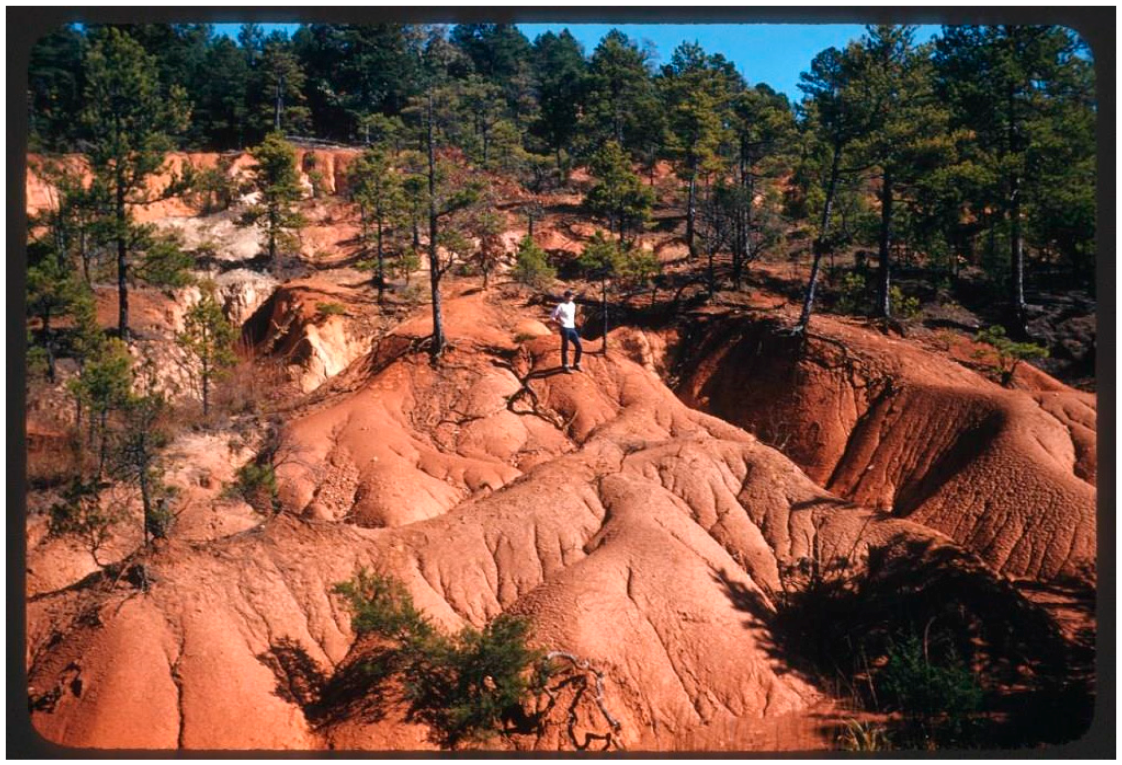
In this paper, we investigate landscape-level relationships between land use change, local socioeconomic conditions that structure use of land (land tenure type, market cost distance), and topographic attributes of the land. To empirically analyze these relationships, we examined a highly degraded landscape (Figure 1) in the South Carolina Piedmont during 1933–1941, a period characterized by land use transitions from intensive plantation agriculture to a forest-dominated private-public patchwork mosaic. The objectives of our research were to (1) quantify the relationships between topography, market distance, and land use change at the parcel-level (e.g., individual land management units); and (2) quantitatively assess the effects of land tenure arrangements and property regime-circumscription of natural resources on household-level land use strategies. We use multinomial logistic and binomial logistic regression modeling approaches to establish relationships between presence and absence of particular land uses in relation to independent landscape conditions. We hypothesize that (H1) farmers’ spatial allocation of land use reflect efforts to optimize production given constraints imposed by topography (a proxy for degradation potential) and topographically weighted distance between fields and markets (a proxy for market-oriented production costs) and (H2) farmers differentially respond to these constraints through placement and abandonment of agricultural fields according to their individual property and land tenure arrangements.
2. Study Area and Background
This investigation was conducted as part of the Calhoun Critical Zone Observatory (CCZO) project, a US NSF Division of Earth Sciences initiative to bring together a wide range of sciences on particular landscapes. The CCZO is an interdisciplinary research field site located on the Calhoun Experimental Forest, itself part of the Sumter National Forest, located in Union County, South Carolina (a 1336 km2 administrative unit). Our study area (roughly, 34°36′40″ N, 81°42′50″ W) encompasses the Calhoun Experimental Forest’s 2057 ha and adds an adjacent 14,143 ha of the surrounding Sumter National Forest for a total surface area of 16,200 ha (Figure 2). The study area is located in the Piedmont plateau physiographic region, bounded by the Appalachian Mountains to the west and the Atlantic Coastal Plain to the east. Topographically the study area is characterized by broad uplands at about 205 m above mean sea level (amsl) that drop steeply down slope into bottomland flood plains at about 95 m a.m.s.l. Current land cover is dominated by forests composed mainly of mixed pine-hardwoods and pine stands both planted and naturally regenerated. The area receives about 1180 mm of precipitation per year and temperatures typically range between −2.4 °C, (average minimum temperature for the coldest month) and 33.1 °C (average maximum temperature for the warmest month).
Historical Context
Piedmont farmers began to orient their productive strategies toward the growing cotton market as early as the 1790s [30]. Although household-level subsistence farming continued in some areas of Union County, by 1820 much of the study area was consolidated into large slave-holding plantations dominated by cotton production. Following the emancipation of the slaves at the end of the US Civil War (ca. 1865), plantations were radically reorganized [31]. Labor relations transitioned to annually renewable share- and fixed-rent tenancy agreements and settlement transitioned to a dispersed, household-centered pattern. Throughout this period, erosional processes triggered by upland, market-oriented cultivation are thought to have led to some of the most extreme degradation in the country, although the exact timing and pace of degradation continue to be investigated.
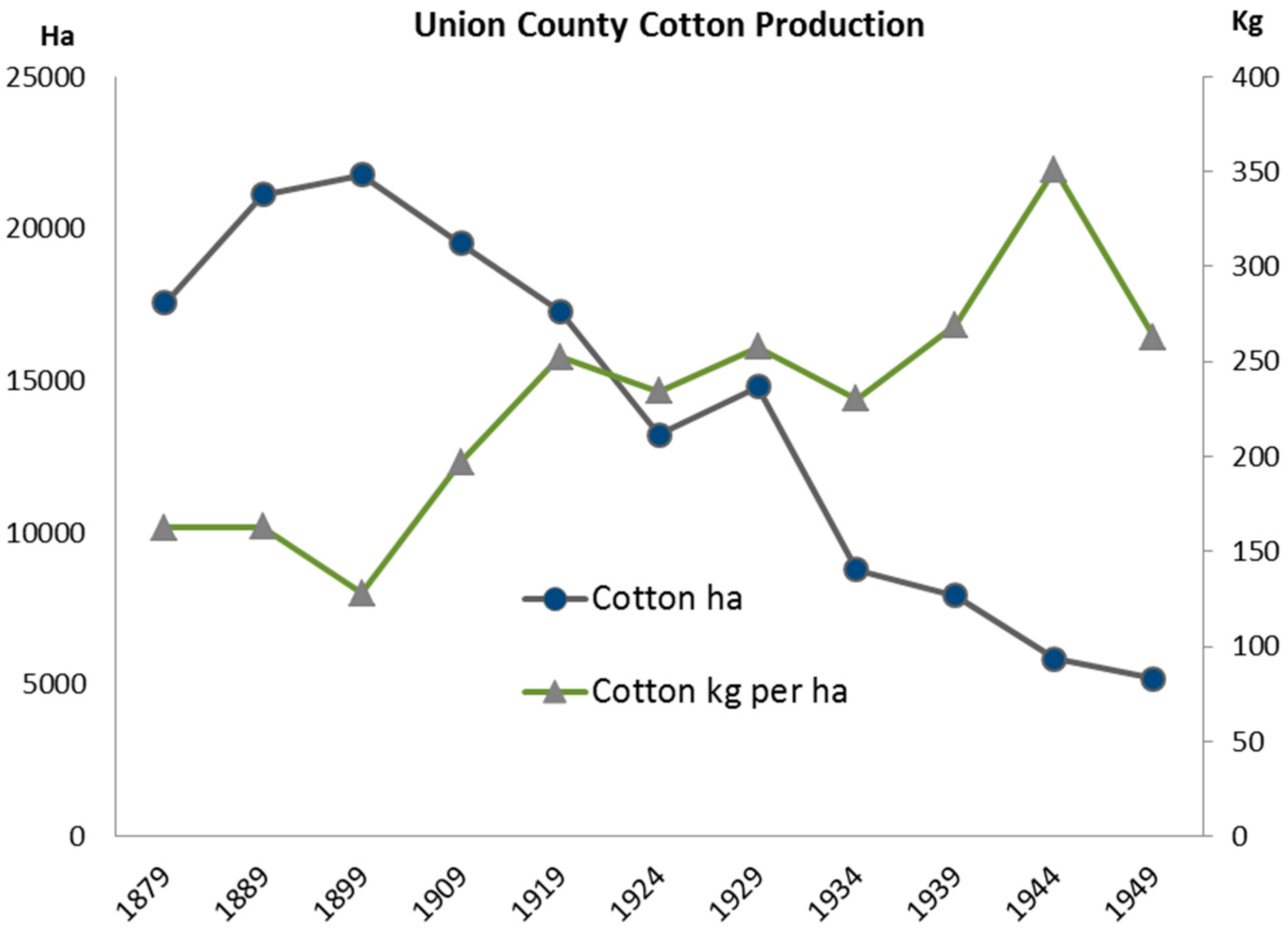
Cotton, followed by corn, was Union County’s primary agricultural export between 1849 and 1949. Cotton covered approximately half of Union County’s fields and corn occupied a quarter, leaving one quarter of the county’s fields for other crops. By 1920, the effects of agricultural improvements and material inputs in the form of fertilizers became evident as cotton yields increased by 27% over its 1889 value while area under cotton cultivation declined by about 30% over the same period (Figure 3). Nonetheless, as is clear from the drastic drop in area planted beginning in 1929, fewer people were choosing to plant cotton. Undoubtedly, unstable cotton markets, increasing costs of production, and pests such as the boll weevil were eroding the socioeconomic foundation of the agricultural system. While limited farming continued after 1949, 18% of Union County is now in forest cover under the stewardship of the federal government, 85% of which is included in the present study.
The intensive land-use practices of cotton-dominated agriculture drastically altered soils and the geomorphology of landscapes in the Piedmont of the southeastern US [32,33,34]. One historian of soil conservation in South Carolina’s Piedmont suggested that, “from the standpoint of conservation the separate elements of the farm-management system were poorly integrated,” due to a legacy of “pioneer era” farming techniques [35] (p. 14). Another explanation for the degradation of the Piedmont hypothesized that areas with more non-owner farm laborers (slaves and, later, tenants) saw the worst erosion due to laborer negligence: “An owner might not see portions of his holdings for months on end, while the workers were engaged in poor cultivation practices,” [30] (p. 411). Environmental geographer Stanley Trimble [32] dismissed this argument suggesting instead that, in addition to frequent heavy rains and rugged topography, Southern land owners lacked a “land ethic”. Others have suggested that the effects of cotton on the soil, inefficient planting and tilling practices, and improper placement of fields, proved a lethal combination for the land [9,36,37]. Whatever the proximal causes of soil degradation, authors appear to agree that Piedmont agricultural strategies were ultimately following a self-reinforcing pathway to socioecological collapse that only state-initiated intervention might begin to solve.
The New Deal solution for the Piedmont, as with many other impoverished areas of the United States during the Great Depression, was a state-sponsored and administrated conservation initiative. It is during the New Deal land purchase era (1933–41) that the US Forest Service began to purchase the area of the Sumter National Forest that would become the Calhoun Experimental Forest, and later the Calhoun CZO (hereafter, “Purchase Era”). In the South Carolina Piedmont, these conservation efforts established the Sumter National Forests and provided federally funded Civilian Conservation Corps (CCC) to construct terraces, fences, conduct fire suppression, plant trees, and fill gullies [38]. On the surface, the conservation initiatives begun during the New Deal era appear to have placed the land on a trajectory of regeneration. Yet, below the surface, the legacies of degradation remain, their trajectories subject to scientific scrutiny [12]. Importantly, however, this narrative ignores the local processes that may already have been leading to ecological regeneration at the time of purchase through processes of agricultural abandonment and natural reforestation. Indeed, it is likely that the reason the National Forest establishment program had such significant buy-in is a function of a locally sourced process that merged with national level policies.
3. Materials and Methods
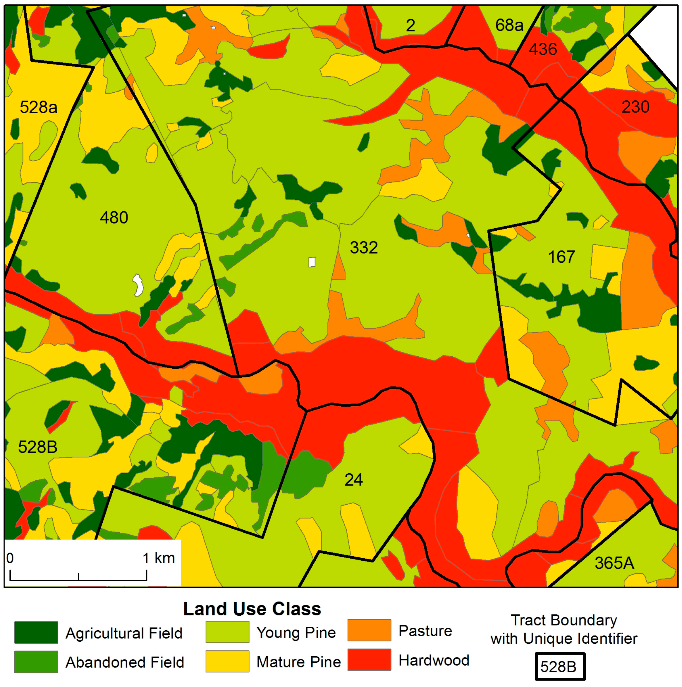
To understand the transition from plantation agriculture to a forest-dominated landscape, we analyze land use and tenure at the time the US government acquired the majority of what became Sumter National Forest, 1933–1941. Our investigation focused on two spatially and conceptually different units of analysis: property ownership or “tract” level and the land management level or “land use unit” (Figure 4). Land use units comprise a contiguous and bounded area of homogenous land use, for example an agricultural field or a woodlot [39]. Tracts are comprised of multiple land use units and constitute contiguous, legally bounded units of land ownership. Tracts are here assumed to be operationally equivalent to individual farms or plantations where landowners singly determine the number, nature, duration, and diversity of land tenure agreements. Land tenure agreements, in turn, define the possibilities and constraints within which individual farmers made their land use decisions.
We conducted two separate statistical analyses to capture the role of biophysical and social factors in determining land use practices in specific locations under specific management arrangements (see supplementary material Table S1 for data, Table S2 for data codes, and Table S3 for analysis instructions). The first analysis is a multinomial logistic regression which assesses associations between land use classes and explanatory variables including physical and material assets, topographic indices, and transportation networks. The second analysis, a binomial logistic regression, captures the influence of social relationships, represented by land tenure arrangements, on land use decisions.
3.1. Tract Condition and Land Tenure
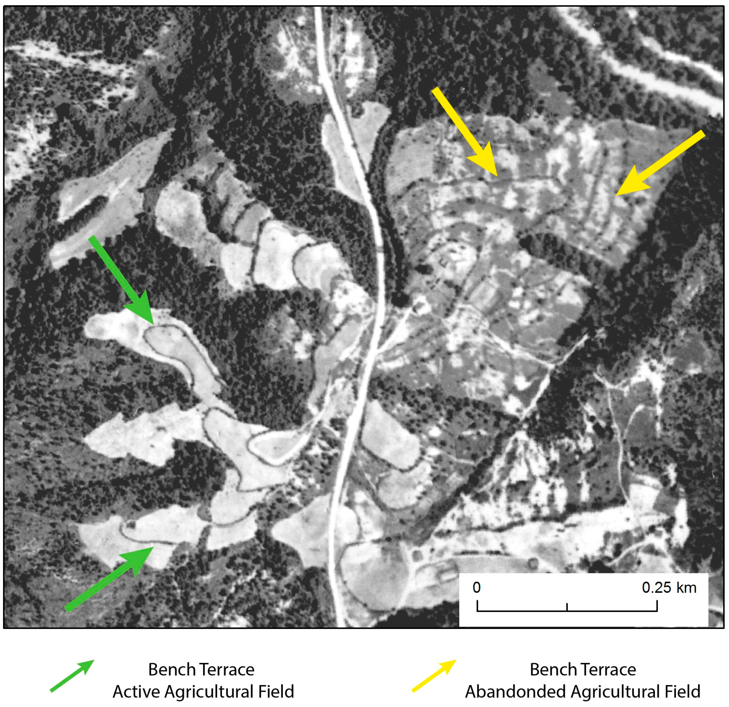
Our data derive from US Forest Service archives that contain legal descriptions, maps, economic assessments, deed abstracts, and other records pertaining to the acquisition of land by the US government during the Purchase Era (1933–1941). Boundaries for 86 tracts were digitized from legal descriptions and maps produced by professional surveyors. Tracts varied widely in ownership, valuation, and ranged in size from 9.2 to 2341.4 hectares (ha) (Appendix A). At the time of purchase, 55 tracts had land use units identified as active agricultural fields. Agricultural fields averaged about 3.7 ha, but ranged from 0.06 to about 45 ha and covered a total of 1120.6 ha, just under 10% of the study area. Overall, tracts purchased by the US Forest Service were either entirely abandoned or had relatively high quality active agricultural land. The highest quality agricultural lands were terraced to conserve soils and even some of this land was already abandoned by 1933 (Figure 5). Only one of the 55 actively farmed tracts is noted as having un-terraced agricultural land. 94% of the severely degraded land was obtained in 1934, the first year of US Forest Service purchase.
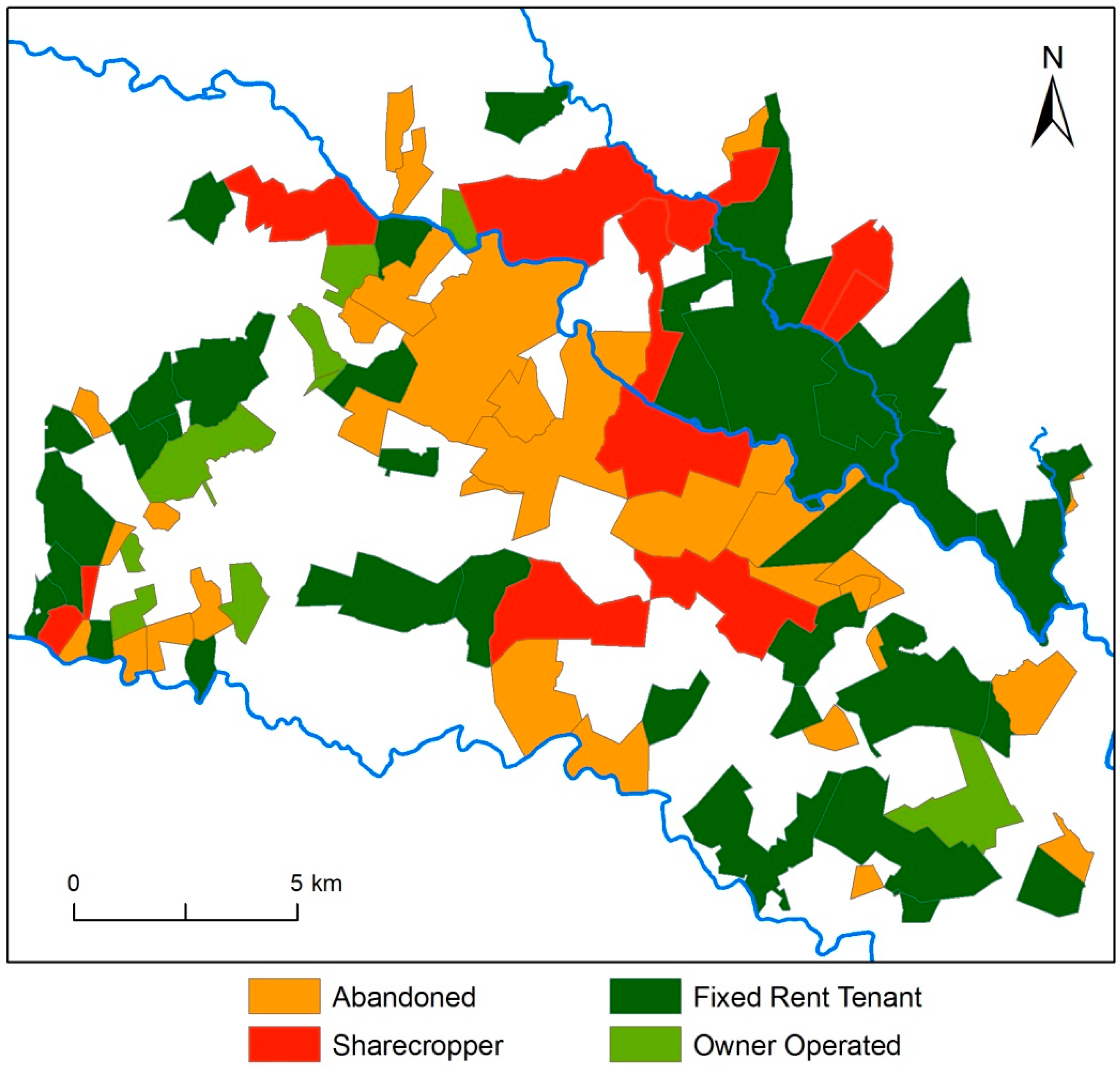
We used Forest Service purchase documentation to characterize the general type of land tenure for tracts in our study area. Thirty-one tracts were entirely abandoned by the time of purchase (classified as “abandoned”). Land tenure on the 55 actively farmed tracts fell into three general categories (Table 1, Figure A1): owner-operated, fixed-rent tenants, and sharecropper tenants. The owner-operated tenure type indicates that the tract owner was actively engaged in farming the tract. Fixed-rent tenants paid a fixed price rent to farm a tract, supplied all of their own equipment and material inputs, but were able to keep any profits they obtained through sale of their agricultural produce [31]. Sharecropper tenants paid a share of their crop, 50% in our study area, to the land owner or a middleman “merchant”.
3.2. Land Use Units
Land use units were digitized from tract-level land use maps created as part of the US Forest Service tract appraisal process. Unit boundaries were cross-validated with a 1933 aerial photo mosaic and, where coverage permitted, a 2014 LiDAR generated digital elevation model (DEM). We used 5 land use classes for this analysis: active agricultural land (land use 1), abandoned agricultural land (land use 2), young pine forest (land use 3), mature pine forest (land use 4), and hardwood forest (land use 5) (Table A3). Active agricultural land (land use 1, 354 observations) includes only plowed crop fields and excludes pastures. Although pastures were classified in the original Forest Service land use assessments, they are not numerous in the study area and represent less than 2.6% of the classified surface area. Additionally, pasture lands present an anomalous and topographically ambiguous land use class as they occurred in both bottomlands and more rugged upland terrain. Abandoned agricultural land (land use 2, 176 observations) includes recently abandoned or fallow fields not yet colonized by pine reproduction. Young pine forest (land use 3, 333 observations) is derived from the original classification as non-appraisable young stands of Loblolly and Shortleaf pine forest. These classifications were based on timber cruise appraisals of both planted and naturally regenerated pine forest with trees less than 10 inches in diameter at breast height with anticipated maturity (70–90 feet in height) within 50 years. This land use class most likely represents abandoned agricultural land with pines greater than three years in age. Based on previous studies of ecological succession in abandoned agricultural fields in the Piedmont, the young pine category represents 3 to 30 years of stand establishment [41,42,43]. Mature pine forest (land use 4, 201 observations) is derived from the original classification as merchantable saw timber. Merchantable pine saw timber had greater than 10 inch diameter at breast height and a top diameter of at least eight inches. However, average per tract height and diameter reported for mature trees ranged between 80–90 feet tall, and 18–24 inches in diameter, depending on the location. Based on these estimations, our classification of mature pine most likely represents an age range between 30 and 75 years, placing stand establishment in the mid- to late-19th century [41]. Finally, the hardwood forest classification (land use 5, 211 observations) was derived by combining all categories of hardwood forest. We employ hardwood forests as a statistical baseline category in the formal analysis in part due to their ability to persist across a broad sweep of ecological conditions. However, hardwood forests are more accurately described as “woodlands” in that they were managed for multiple uses, supplying firewood, timber, and other forest products. In addition, many hardwood stands were used as woodland pastures for cattle, sheep, goats, and pigs. The 1925 and 1930 agricultural census for active farms in Union County shows woodland pasture as 12.2% (3397 ha) and 15.6% (3164 ha) of total farm woodlands respectively. The hardwood forests land use class within our study area represents 15.6% of the total area of forested land use classes.
3.3. Topographic Indicies
Gully and sheet erosion were among the most serious aspects of land degradation across the Piedmont [33,37]. Although land use change can trigger erosion, surface topography is a significant contributing factor. Indeed, slope and soil moisture in particular are known to predispose a landscape to gully erosion [44]. We used a 10 m × 10 m USGS seamless Digital Elevation Map (DEM) to extract slope and to construct a Topographic Wetness Index (TWI) and a Relative Topographic Position index (RTP). The Topographic Wetness Index provides an estimate of soil moisture whereas the Relative Topographic Position Index provides a way to classify topography in relation to its position in the landscape (e.g., bottomland, side slope, and uplands). TWI was calculated by dividing the natural log of the contributing area by the slope of an individual raster cell [45]. The Relative Topographic Position Index classifies each pixel in a raster with reference to its neighborhood [46]. RTP was calculated with minimum, maximum, and smoothed elevations in 10 × 10 cell neighborhood (e.g., 100 m × 100 m) following the formula (smoothed DEM − minDEM)/(maxDEM − minDEM). The resulting continuous raster was then classified using Jenk’s natural breaks into 3 categories representing: (1) wider bottomlands; (2) narrow ridges, ravines, and side slopes; (3) broad interfluvial uplands. We extracted the mean and standard deviation of slope for each land use unit-level in order to calculate the coefficient of variation (standard deviation/mean) for slope. The slope coefficient of variation (Slope CV) provides a land use unit-scaled measure of its topographic variability where high values signify more rugged terrain and low values signify less rugged terrain.
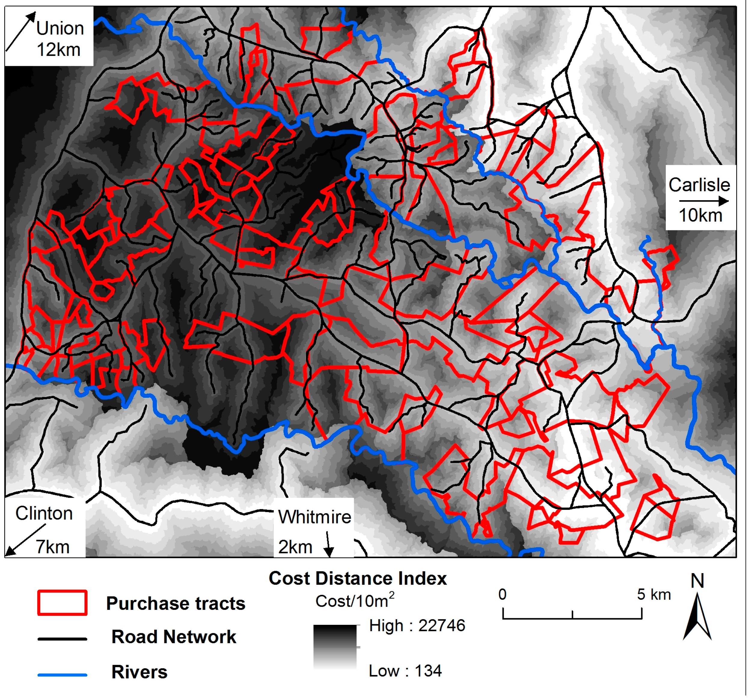
As a proxy for the effects of differential access to markets (central-place market forces) [7,20,47], we constructed a nearest market Cost-Distance Index (CDI). This index represents the geographically weighted cost of transporting farm products and materials to and from market. To construct the Cost-Distance Index we digitized the Purchase Era road network by adapting the existing road network to the 1933 aerial photo mosaic. We calculated cost-distance as the slope-weighted distance from a 10 m × 10 m node or “pickup” point on the road network to one of the nearest of four market towns surrounding the study area (Clinton, Whitmire, Union, and Carlisle) by following the least-cost road route from the pickup point to the market town. To account for differences in road quality, the roads were additionally weighted in two grades, primary = 1, secondary = 2. Primary roads were publicly-maintained highways that directly connected the market towns with each other and secondary roads linked farms to highways. We combined the road network-based cost-distance with a field-specific cost-distance analysis. The field-specific component calculated the slope weighted distance from a 10 m × 10 m area to its nearest pickup point along the road network. We combined both layers into an aggregated cost-distance index by adding the field-based cost-distance to the road network cost-distance for its assigned (nearest) pickup point (Figure 6). We then calculated the average cost-distance values for each land management unit to serve as covariates in the formal analyses.
3.4. Statistical Analyses
3.4.1. Multinomial Logistic Regression of Land Use Class
In order to infer the relationship between Purchase Era land use and the landscape we characterized the distribution of our land use classification across the five topographic parameters described above. We selected a multinomial logistic regression (M-logit) [48] to predict the probability of a field belonging to a particular land use class, given topographic characteristics. M-logit is suited to analyses where the dependent variable Y has k possible values. Each possible Yk, in our case a land use class such as an agricultural field, is compared to a “baseline” class (Y1). The M-logit model for the log odds is written
where βi refers to the effect of xi (a particular topographic feature such as slope) on the log odds that dependent variable is Yk (land use class) relative to Y1. The equation is repeated for each condition of Y [49,50]. We used hardwood forest as our baseline land use class (Y1). Our independent variables (xi) were at land use unit-level and consisted of mean slope, mean topographic wetness, mean cost-distance, and the coefficient of variation for slope. All independent variables were normalized based on the overall mean and standard deviation and checked for collinearity. Interrelationships between all independent variables yielded a Pearson’s correlation coefficient R value of less than 0.5.
ln (P(Yk)/P(Y1)) = α + β1x1 + β2x2 +· · ·+ βkxk,
We used Stata (release 11.2) to conduct the M-logit and report the relative risk ratio (rr ratio) as a measure of the effect of the independent covariates on the dependent variable (land use class). In contrast to an odds ratio, which is the ratio of two odds, the rr ratio is a ratio of two probabilities. It denotes the ratio of the likelihood of a land use class being Yk (e.g., agricultural field) to the likelihood that it is the baseline class Y1 (hardwood forest), for each one unit increase in covariate. An rr ratio > 1 indicates a greater likelihood for Yk whereas rr ratio < 1 indicates greater likelihood for Y1. An rr ratio = 1 would indicate that the independent variable had no effect on the dependent. Therefore, the closer the rr ratio is to 1, the weaker the effect. We additionally report a McFadden pseudo R2 as a goodness of fit measure and used a 5% significance level for both the model fit (Probability > Chi-squared) and for the individual correlation coefficients (p-value). McFadden pseudo R2 typically yields lower values than an OLS R2 and results between 0.2 and 0.4 are considered indicative of excellent model fit [51].
3.4.2. Binomial Logistic Regression of Agricultural Land by Land Tenure
We used a standard binomial logistic regression model (logit) to test for differences in agricultural land use at the tract level. Differences in land tenure arrangements constrain and incentivize farmers’ decisions concerning the location and class of land use. Our logit model included a binary response variable indicating presence versus absence of active agricultural use where active agricultural fields were assigned a value of “1” whereas all other land use classes were assigned a “0”. Independent covariates were the same standardized variables from the M-logit analysis. To test for differences in land use strategies between tracts, we used the “by” function to obtain unique coefficients and p-values for each land tenure type. One possible drawback of this method is that it assumes a priori independence between each resulting subset of the dependent variable.
As in the M-Logit analysis, we used a 5% significance level to evaluate the model. For the logit results, we report the odds ratio which indicates (holding all other things constant) the direction and amount of change in the dependent variable given a one unit increase in the independent variable.
4. Results
4.1. Land Use Unit-Level Statistical Analysis: M-Logit
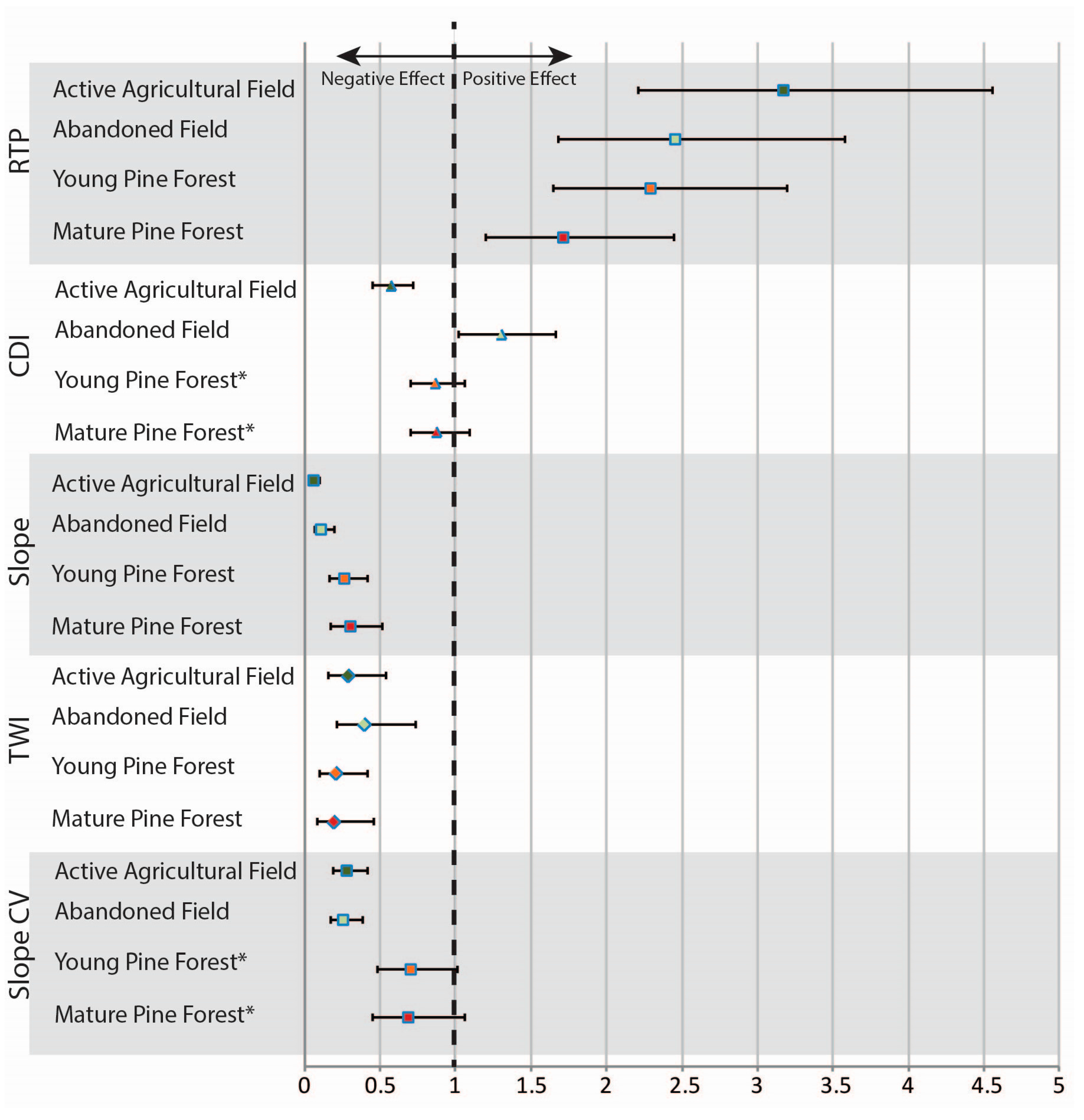
The Pseudo R2 for the M-Logit was 0.20 which indicates an acceptable fit for this type of model [51]. The relative risk ratios varied across the land use classes for each of the five independent variables. Analysis using the Relative Topographic Position indicator provided insight on the most probable location (uplands; ravines and side slopes; or bottom lands) of different land uses. The relative risk ratios for relative topographic position were significant and the strength of its effect varied across land use along a gradient consistent with studies of ecological succession in the Piedmont (Figure 7). The strongest, positive association is between agricultural fields and uplands. The gradient then follows to abandoned fields, young pine forest, and mature pine forests, each with a decrease in the strength of the relationship in comparison to baseline hardwood forests.
The cost-distance covariate assesses the strength of association between a land use class and the cost-weighted distance from markets. It was only statistically significant for active and abandoned agricultural fields. Active agricultural fields were negatively associated with increases in cost-distance from the nearest market while abandoned fields were positively associated with increasing cost-distance. Thus, higher cost-distances likely influence decisions to abandon one field over another.
Results for Land use unit-level mean slope were consistently significant across land use classes with an incremental increase in slope predicting for hardwood forest over all land uses (Figure 7). In aggregate, there is an inverse relationship between slope and the presence of agricultural land, active or abandoned: the higher the slope, the less likelihood the land was in agricultural production. Land use followed a gradient of sensitivity to slope that starts with agricultural fields with the highest sensitivity to abandoned fields to young pine and to mature pine with the lowest sensitivity. Given the temporal dimension to these land use categories hypothesized by studies of ecological succession, our results suggest that steeper agricultural fields were the first to be abandoned and allowed to reforest.
The mean topographic wetness covariate had mixed significance (Figure 7). The relative risk ratio for topographic wetness indicates that incremental increases in wetness favored hardwood forest over the other land use classes. However, this effect was weakest for abandoned fields, meaning that abandoned fields were more likely to be in potentially wet soils than active agriculture or pine forests. This result may reflect relatively recent abandonment of wetter bottomlands following erosion-induced sediment inundation of topsoils. It also shows that both young and mature pine forests were situated in potentially drier soils than those of active and abandoned agricultural fields.
At a 100 m 2 resolution, hardwood forests had the highest topographic variability of all land use classes. Placement of agricultural fields (active and abandoned) was considerably more sensitive to incremental increases topographic variability than young and mature pine. The relative risk ratio for active and abandoned agricultural fields were similarly associated with less rugged terrain, while both young and mature pine forests shared a similar association with more rugged terrain. Thus, if rugged areas were used for agriculture, they were long abandoned by the Purchase Era.
4.2. Placement of Agricultural Land by Land Tenure: Logit
Pseudo R2 results for each land tenure were all relatively high (>0.24). Land use unit-level mean slope was the only factor significant across all land tenure types. Results followed a gradient of increasing negative effects on the presence of active agricultural fields: sharecrop < fixed-rent tenant < abandoned < owner operated (Table 2). Cost-distance, although not significant for owner-operated tracts, showed strong positive effects on the presence of (recently abandoned) agricultural fields in abandoned tracts and mostly similar, smaller, and negative effects on the active agricultural fields in other land tenure types. Thus, agricultural fields on abandoned tracts were less steep and less topographically variable but had the highest cost-distance. Sharecroppers were farming the most marginal areas (steep and narrow ridges) while owner-operated tracts had agricultural fields located in the broadest and most level areas.
5. Discussion
If piedmont farmers were “inefficient” in their planting practices or if they had improper placement of fields we would expect to see mismatches between land use and topographic factors. Instead, our results confirm our hypothesis (H1) that farmers allocated land use across the landscape in ways that optimized productive potential given topographic and distance constraints. This suggests that piedmont farmers of the 1933–1941 Purchase Era understood their social and ecological environment and were not ignorant “soil miners”. US Forest Service property valuation documents demonstrate that by the Purchase Era, the majority of the study area’s farmers were terracing and ditching to cope with soil degradation and accelerated erosion. Further, according to the US Forest Service valuations, fields remaining under cultivation were well cared for, regardless of land tenure arrangements. Indeed, the valuations indicated that the most severely degraded agricultural lands were found on abandoned tracts. In support of these conclusions, the M-logit results suggest that fields more topographically susceptible to degradation (steep, dry, and topographic rough slopes) underwent reforestation well before the Purchase Era.
Our results also support our hypothesis (H2) that farmers differentially responded to the cascading effects of land degradation and market forces according to the constraints imposed by farm attributes and land tenure arrangements. Land tenure arrangements constrained farmers’ ability to respond to both changes in external socioeconomic conditions as well as the more local feedback of land degradation. For example, sharecroppers were more likely to farm steeper slopes on narrower ridgetops than either fixed-rent tenants or owner operators. Sharecropper tracts had the lowest sensitivity to market cost-distance for active agricultural fields, but also the largest percentage of abandoned agricultural fields. This suggests that sharecroppers may have been more sensitive to changes in market price, since they experienced higher costs of transporting fertilizers from and produce to markets. However, lacking security in land tenure they were also more mobile than other farmers and could more readily abandon fields. As a consequence, sharecropped farms economically more costly to operate were likely to be the first abandoned. Tract abandonment occurred where the entire tract was costly in comparison to its neighbors. Conversely, farmers with the highest land tenure security (e.g., owner-operated farms) were tied to their properties and continued to farm fields in spite of their higher economic costs. We elaborate on these insights and their implications for understanding landscape transition at the Calhoun CZO in the following discussion.
5.1. Effects of Topography and Market Cost-Distance on Landscape Transition
Hardwood and mature pine stands were predominant in areas with the steepest and most variable slopes, areas highly susceptible to agriculturally induced land degradation. If these areas were cleared for farming, they were abandoned by the Purchase Era, some as early as the 1860s and 1870s during the post-Civil War Reconstruction era. This analysis is also consistent with the 1933 aerial photo interpretation by Brecheisen et al. [17] that agricultural land appears predominantly on broad, gentle sloped ridgetops. Some areas, specifically the upland hardwood forests may have been reserved from agricultural uses due to increasing scarcity-driven hardwood timber values from the mid-1800s forward [30]. Given that steep and topographically rugged areas were also the most difficult to clear and farm, it seems likely that these stands were rarely if ever cultivated. Thus, in terms of settlement-abandonment dynamics, the last places to be farmed would have been the first places to be abandoned.
Socioeconomic effects are evidenced in both analyses through the cost-distance results. In the M-logit, cost-distance is only positively associated with abandoned agricultural fields. In the logistic regression, “abandoned” tracts showed a positive relationship between cost-distance and agricultural fields, indicating that abandoned tracts tended to have high market cost-distance in comparison to actively farmed tracts. Yet topographic constraints on abandoned tracts were similar to tenant-operated tracts. In other words, farmers in recent years were likely disadvantaged more by cost-distance than degradation and responded by abandoning fields and entire farms. Perhaps counter intuitively, young pine does not show a positive association with cost-distance. However, young pine is associated with steeper, dryer slopes and more rugged terrain than either active or abandoned agricultural fields. Likely, there may be a threshold effect where topographic constraints become more important than market cost-distance and vice versa. Alternatively, since the young pine category represents an earlier phase of agricultural abandonment, topographic constraints may have been more important than cost-distance at that time. Changes in transportation technology or the road network could account for such a shift.
Our results make clear that farmer decisions were influenced by topographic and spatial constraints specific to each farm. For areas with more recent land abandonment (less than 3 years) evidenced by the “abandoned field” land use class, the analysis shows that these areas too were topographically more susceptible to degradation than fields that were retained in active agricultural use. This result raises the possibility that at least some farmers were responding to the Agricultural Adjustment Act of 1933, which paid farmers to reduce cotton production. Although cotton acreage was reduced, yields increased, ostensibly due to the concentration of fertilizers and labor on remaining higher quality acreage [52]. Indeed, by the time of the US Forest Service land purchase, farmers in our study had abandoned more marginal fields and either migrated elsewhere or, where it was available, focused on the terraced, “above average” farmland that remained.
With the more highly-degraded lands now out of production and the remaining fields improved with terraces and ditches, land owners and tenant farmers might have chosen to continue cotton farming. However, in 1934, the government passed an additional law, the “Bankhead Cotton Act” which imposed a prohibitive tax of 50% of the price on cotton in excess of the “assigned quotas” [53]. The Bankhead Act and the opportunity to sell more marginal lands to the US Forest Service likely influenced the decisions to opt out. Only farms with the choicest fields remained in production.
5.2. Land Tenure and Responses to Land Degradation
Investments in agricultural inputs and improvements such as the application of commercial fertilizers, [ditching, and terracing, in response to agriculturally induced erosion in the Piedmont began as early as the mid-1800s [37,54]. The wide bench terraces evident in a 1933 aerial photo of the Calhoun CZO (e.g., Figure 5) and noted in the US Forest Service economic valuation reports probably date from the 1890s onward [54]. These solutions were widely viewed as successful in the fight against erosion and, at least in our study area, there were few cultivated areas without such terraces by the Purchase Era.
However, terracing and ditching may also have exacerbated gullying in the areas immediately downslope as water was channeled off the bench terraces onto steep hillslope soils and gullies [37]. Indeed, infrastructural investment in terraces and drainage ditches appears to have been made at the field, rather than plantation or landscape level. Despite being forested, uncultivated steep hillslopes eroded severely. In addition, ditch and terrace systems required maintenance and, if not maintained, exacerbated erosion [48,55]. Thus, it remains difficult to determine the extent to which degradation caused abandonment or vice versa.
Efforts to conserve and improve soils and to maintain such investments most likely varied between property and land tenure types. Farmers with less secure land tenure may have been less willing to implement long term solutions since their future access to the land remained uncertain. Since sharecroppers were farming areas more susceptible to erosion than their neighbors, but also had the least incentive to invest in their land, this situation may have inevitably led to degradation. As noted above, insecurity in land tenure brought a higher degree of mobility. Thus, as fields were exhausted and eroded, sharecroppers probably moved to other fields and plantations or gave up farming altogether in order to pursue wage work in towns and cities. Uncertain land tenure in the most marginal lands likely proved a lethal combination for soils as socioeconomic incentives focused improvements on fields rather than farms and encouraged abandonment rather than the maintenance of improvements.
Owner-operator farmers faced different constraints. Their agricultural fields were located on the most level and widest interfluves. We also observed in the process of digitizing the land use data that most of the few bottomlands being actively farmed during the 1930s were on owner-operated tracts. These bottomland fields were narrow, located in lower order stream bottoms, away from the highest order, wide river bottoms. Historically, bottomland terraces of the Enoree and Tyger Rivers and their tributaries were known for their fertile soils [35]. However erosional deposition caused by degradation of upland soils, heavy rains, and flooding deposited a meter or more of sediment on higher order bottomlands, rendering them largely unfarmable [56]. The bottomlands of lower order streams within owner-operated farms may have escaped some of the worst sedimentation due to better land stewardship and smaller catchments. In maintaining fields in these bottomlands, owners may have increased their resilience to market forces. The continued, but limited use of bottomlands may also explain why results obtained in the logistic regression for the cost-distance and topographic wetness covariates were not significant for owner-operated farms.
6. Conclusions
The degradation of ecosystem services is a key challenge of our time [53,57]. The dynamic human-environment relationships that drive land use-caused degradation are reciprocally interactive at the individual and landscape scale. Our ability to successfully address change requires detailed understanding of land use transitions at multiple scales, including managed transitions as well as emergent transition processes [58]. Our study focuses on the ways in which individuals make land use decisions within local physical and social contexts. In the 1930s, degradation of the Piedmont was severe and intervention by the US Forest Service may have been a necessary step toward regeneration of vital ecosystems services. However, prior to this intervention, farmers were already responding to degradation through changes in land use. Notably, by the 1930s, farming had retreated from the areas most susceptible to degradation. Indeed, we argue that many of the factors and processes that facilitated the state-led forest transition in the 1930’s and 40’s were already emerging prior to state intervention. We demonstrate that farmer’s options and abilities to respond were a function of the physical characteristics of individual landholdings and social circumstance. In other words, farmers make decisions, not based on a regional landscape, but rather, situated in the particular characteristics of their own landholdings and socioeconomic circumstances. They assess these characteristics, based on an understanding of their own socially constrained possibilities. These insights are crucial for understanding spatial heterogeneity in the legacies of land degradation, obscured in broad-scale analyses of land use transitions.
Consistent with other studies of land use transition, our place-based, historical analysis demonstrates that biophysical factors, such as topography and market cost-distance, influence land use practices and timing of land abandonment [10,11,59,60,61,62]. But, critically, this relationship is not identical among all farmers. Rather, the characteristics of feedbacks between soil degradation and erosion on farming decisions are fundamentally a function of socially determined land tenure systems, though not always in an intuitive fashion. Our findings demonstrate, for example, that the mobility associated with insecure land access provides a different set of response options than that for land-owners, who are fixed in place and make land management decisions within the non-negotiable constraints of property boundaries. As a consequence, we suggest that land use policy aimed at improving environmental conservation and human wellbeing must explicitly consider the local constraints and dynamics introduced by land tenure, property regime, and cost-distance to markets.
Supplementary Materials
The following are available online at www.mdpi.com/2073-445X/6/2/32/s1, Table S1: Logistic Regression Data, Table S2: Code Sheet, Table S3: Analysis Instructions.
Acknowledgments
The research and open access fees were funded by a grant from the United States National Science Foundation (NSF# EAR-1331846) Critical Zone Observatory program. We thank the US Forest Service and Sumter National Forest, Enoree District archaeologist Mike Harmon for providing assistance and access to historical archives. We thank Calhoun CZO investigators Dan Richter and Zach Brecheisen for their helpful comments and Mukesh Kumar for his technical advice with DEM analysis. Lastly, we dedicate this paper to the memory of Ashley Block who contributed greatly to the research efforts behind this paper.
Author Contributions
M.C. and D.N. conceived and designed the research; M.C. conducted the analysis; M.C., D.N., M.L., and A.B. contributed data, interpretations of analysis, and wrote the paper.
Conflicts of Interest
The authors declare no conflict of interest. The funding sponsors had no role in the design of the study; in the collection, analyses, or interpretation of data; in the writing of the manuscript, and in the decision to publish the results.
Appendix A
A.1. Land Tenure Typology
At the tract level, land tenure types were not mutually exclusive as any given tract might have a combination of different land tenure arrangements. For example, two owner-operated tracts also had sharecropper tenants and two tracts had both fixed-rent and sharecropper tenants. For statistical analysis at the tract level, we required a mutually exclusive land tenure categorization (Figure A1). Consequently, we simplified land tenure by reasoning that importance of land tenure to land degradation would follow the relative degree of socioeconomic investment such that: owner operated > fixed-rent tenant > sharecropper > field renter. So if an owner-operated tract also had a sharecropper, the tract was nevertheless classified as “owner-operated”. Field renters (5 households on 6 tracts) rented one or more fields on a tract and either owned or rented a “home” farm on another tract. As a consequence, tracts with field renters were classified according to the predominant tenure for home farms on the tract (see below).
Figure A1.
Tracts in study area classified by land tenure type (1933–1941).

A.2. Tract Ownership and Valuation
We located US Forest Service land valuation reports for 81 of the 86 purchase tracts. Only 18 of the 55 actively farmed tracts included areas identified as “Below Average” or “Impaired” (Table A1).

Table A1.
US Forest Service valuation of agricultural land.
| Active Agricultural Land Condition | ||||||||
|---|---|---|---|---|---|---|---|---|
| Above Average | Below Average | Impaired, Not Severe | Impaired, Severe | |||||
| Acquisition Year | # of Tracts | Total Ha | # of Tracts | Total Ha | # of Tracts | Total Ha | # of Tracts | Total Ha |
| 1934 | 23 | 353.1 | 12 | 85 | 3 | 40.1 | 2 | 17 |
| 1935 | 21 | 371.9 | 1 | 9.3 | 0 | 0 | 0 | 0 |
| 1936 | 5 | 79.3 | 1 | 4 | 0 | 0 | 0 | 0 |
| 1938 | 4 | 107.2 | 1 | 21.4 | 0 | 0 | 0 | 0 |
| 1939 | 1 | 9.7 | 1 | 2 | 0 | 0 | 0 | 0 |
| 1941 | 0 | 0 | 2 | 12.9 | 1 | 7.7 | 0 | 0 |
| Total | 54 | 921.2 | 18 | 134.6 | 4 | 47.8 | 2 | 17 |
| % Total | 82.2% | 12.02% | 0.04% | 0.02% | ||||
Tract ownership (Table A2) shows that private individuals or families held the vast majority of land at the time of US Forest Service purchase, though many of these were delinquent on taxes or undergoing bankruptcy procedures. However, less than 5% of the purchased land area was situated on owner-operated tracts, and these were the smallest and least variable in area (average 85.9 ha with standard deviation of 76.3 ha). Sharecropped tracts were largest on average (236.2 ha), but covered only 26% of the study area. Fixed-rent tenancy occupied 48% of the surface area with medium sized tracts (151.8 ha). Lastly, approximately 20% of the land was occupied abandoned tracts averaging 130.1 ha, but these tracts had the lowest percentage (71%) of agricultural lands in the “above average” class. In contrast, owner-operated and sharecropper tracts each had 77% of agricultural land classified as above average. Sharecropper tracts showed the highest percentage of recently abandoned land at 43% while owner-operated and fixed-rent tenant tracts showed the least amount of abandonment at 20% each. Very small percentages of severely impaired land were apparent on abandoned tracts (2.4%) and fixed-rent tenant tracts (0.7%). Tracts were also quite variable with respect to per ha value: mean per ha value = US$17 and standard deviation of per ha value = US$15 (Purchase Era currency valuation). Abandoned tracts had the lowest per ha value (US$12), followed by Owner-Operated tracts (US$13), and Sharecropped and Fix Rent Tenant tracts with the same per ha value (US$16).
Table A2.
1933–1941 Land ownership (ha) by land tenure agreement.
| Ownership Type | Abandoned | Sharecropper | Fixed-Rent Tenant | Owner Operated |
|---|---|---|---|---|
| Private Individual | 51,089.82 | 65,748.65 | 110,638.70 | 12,746.54 |
| Bank | 3073.85 | 10,099.03 | 19,966.84 | 0 |
| Charity | 5105.28 | 0 | 0 | 0 |
| Land Corporation | 758.75 | 0 | 9195.95 | 0 |
| Timber Company | 0 | 0 | 784.62 | 0 |
A.3. Land Use Classification
The US Forest Service land use classification provided 9 categories. In addition, the classification differentiated between merchantable and non-merchantable timber stands based on timber height and diameter making 21 potential land use categories. For this analysis, we simplified the classification into 5 classes: active agricultural land (land use 1), abandoned agricultural land (land use 2), young pine forest (land use 3), mature pine forest (land use 4), and hardwood forest (land use 5) (Table A3).
Table A3.
1933–1941 US Forest Service land use classification.
| Original Description | Map Code | Quality | Analysis Code ( ) and Class | Proportion of Landscape |
|---|---|---|---|---|
| Bottomland Hardwood and Hardwood Swamp | HS | Merchantable & Nonmerchantable | (5) Hardwood | 1563.1 ha 12.9% |
| Upland Hardwood | UH | Merchantable & Nonmerchantable | (5) Hardwood | |
| Hardwood | H | Merchantable & Nonmerchantable | (5) Hardwood | |
| Pine/Hardwood | PH | Merchantable & Nonmerchantable | (5) Hardwood | |
| Shortleaf Pine | SL | Merchantable | (4) Mature Pine | 1522.3 ha 12.6% |
| Loblolly Pine | LB | Merchantable | (4) Mature Pine | |
| Mixed Pine (Shortleaf dominant) | SL-LB | Merchantable | (4) Mature Pine | |
| Mixed Pine (Loblolly dominant) | LB-SL | Merchantable | (4) Mature Pine | |
| Shortleaf Pine | SL | Non-merchantable | (3) Young Pine | 6941.8 ha 57.3% |
| Loblolly Pine | LB | Non-merchantable | (3) Young Pine | |
| Mixed Pine (Shortleaf dominant) | SL-LB | Non-merchantable | (3) Young Pine | |
| Mixed Pine (Loblolly dominant) | LB-SL | Non-merchantable | (3) Young Pine | |
| Abandoned Field | FA, FR | NA | (2) Abandoned Agricultural Field | 422 ha 3.5% |
| Cultivated Field | FC | NA | (1) Agricultural Field | 1318 ha 10.9% |
| Pasture/Meadow (grass field) | FG | NA | Excluded | 314.5 ha 2.6% |
| Structure | Symbol | NA | Excluded | 14 ha 0.1% |
| Cemetery | Symbol | NA | Excluded |
References
- Vitousek, P.M.; Mooney, H.A.; Lubchenco, J.; Melillo, J.M. Human domination of earth’s ecosystems. Science 1997, 277, 494–499. [Google Scholar] [CrossRef]
- Ellis, E.C. Anthropogenic transformation of the terrestrial biosphere. Philos. Trans. A Math. Phys. Eng. Sci. 2011, 369, 1010–1035. [Google Scholar] [CrossRef] [PubMed]
- Steffen, W.; Crutzen, P.J.; McNeill, J.R. The anthropocene: Are humans now overwhelming the great forces of nature? Ambio 2007, 36, 614–621. [Google Scholar] [CrossRef]
- Banwart, S.; Chorover, J.; Gaillardet, J.; Sparks, D.; White, T.; Anderson, S.; Aufdenkampe, A.; Bernasconi, S.; Brantley, S.; Chadwick, O. Sustaining Earth’s Critical Zone Basic Science and Interdisciplinary Solutions for Global Challenges; University of Sheffield: Sheffield, UK, 2013; p. 47. [Google Scholar]
- Turner, B.L.; Lambin, E.F.; Reenberg, A. The emergence of land change science for global environmental change and sustainability. Proc. Natl. Acad. Sci. USA 2007, 104, 20666–20671. [Google Scholar] [CrossRef] [PubMed]
- Foley, J.A.; DeFries, R.; Asner, G.P.; Barford, C.; Bonan, G.; Carpenter, S.R.; Chapin, F.S.; Coe, M.T.; Daily, G.C.; Gibbs, H.K. Global consequences of land use. Science 2005, 309, 570–574. [Google Scholar] [CrossRef] [PubMed]
- Lambin, E.F.; Meyfroidt, P. Land use transitions: Socio-ecological feedback versus socio-economic change. Land Use Policy 2010, 27, 108–118. [Google Scholar] [CrossRef]
- Batie, S.S. Soil conservation in the 1980s: A historical perspective. Agric. Hist. 1985, 59, 107–123. [Google Scholar]
- Metz, L.J. The Calhoun Experimental Forest; Southeastern Forest Experiment Station: Asheville, NC, USA, 1958. [Google Scholar]
- Overmars, K.P.; Verburg, P.H. Analysis of land use drivers at the watershed and household level: Linking two paradigms at the Philippine forest fringe. Int. J. Geogr. Inf. Sci. 2005, 19, 125–152. [Google Scholar] [CrossRef]
- Bürgi, M.; Hersperger, A.M.; Schneeberger, N. Driving forces of landscape change-current and new directions. Landsc. Ecol. 2004, 19, 857–868. [Google Scholar] [CrossRef]
- Jepsen, M.R.; Kuemmerle, T.; Müller, D.; Erb, K.; Verburg, P.H.; Haberl, H.; Vesterager, J.P.; Andrič, M.; Antrop, M.; Austrheim, G. Transitions in European land-management regimes between 1800 and 2010. Land Use Policy 2015, 49, 53–64. [Google Scholar] [CrossRef]
- Mather, A.S.; Needle, C.L. The forest transition: A theoretical basis. Area 1998, 30, 117–124. [Google Scholar] [CrossRef]
- Callaham, M.; Richter, D.; Coleman, D.; Hofmockel, M. Long-term land-use effects on soil invertebrate communities in southern piedmont soils, USA. Eur. J. Soil Biol. 2006, 42, S150–S156. [Google Scholar] [CrossRef]
- Li, J.; Richter, D.D. Effects of two-century land use changes on soil iron crystallinity and accumulation in southeastern piedmont region, USA. Geoderma 2012, 173, 184–191. [Google Scholar] [CrossRef]
- Richter, D.D.; Markewitz, D.; Heine, P.R.; Jin, V.; Raikes, J.; Tian, K.; Wells, C.G. Legacies of agriculture and forest regrowth in the nitrogen of old-field soils. For. Ecol. Manag. 2000, 138, 233–248. [Google Scholar] [CrossRef]
- Brecheisen, Z.S.; Halpin, P.N.; Moon, S.; Richter, D.D. Ordering interfluves: Landscape patterns in critical zone structure and evolution. In preparation.
- Perz, S.G. Grand theory and context-specificity in the study of forest dynamics: Forest transition theory and other directions. Prof. Geogr. 2007, 59, 105–114. [Google Scholar] [CrossRef]
- Evans, T.P.; Manire, A.; de Castro, F.; Brondizio, E.; McCracken, S. A dynamic model of household decision-making and parcel level landcover change in the eastern amazon. Ecol. Model. 2001, 143, 95–113. [Google Scholar] [CrossRef]
- Brondizio, E. Landscapes of the past, footprints of the future: Historical ecology and the study of contemporary land use change in the amazon. In Time and Complexity in Historical Ecology: Studies in the Neotropical Lowlands; Balée, W.L., Erickson, C.L., Eds.; Columbia University Press: New York, NY, USA, 2013. [Google Scholar]
- Coughlan, M.R.; Gragson, T.L. An event history analysis of parcel extensification and household abandonment in Pays Basque, French Pyrenees, 1830–1958 AD. Hum. Ecol. 2016, 44, 65–80. [Google Scholar] [CrossRef]
- Van Gils, H.A.M.J.; Ugon, A.V.L.A. What drives conversion of tropical forest in carrasco province, Bolivia? Ambio 2006, 35, 81–85. [Google Scholar] [CrossRef]
- Robbins, P. Political Ecology: A Critical Introduction; John Wiley & Sons: New York, NY, USA, 2011. [Google Scholar]
- Godoy, R.; Jacobson, M.; De Castro, J.; Aliaga, V.; Romero, J.; Davis, A. The role of tenure security and private time preference in neotropical deforestation. Land Econ. 1998, 74, 162–170. [Google Scholar] [CrossRef]
- Hettig, E.; Lay, J.; Sipangule, K. Drivers of households’ land-use decisions: A critical review of micro-level studies in tropical regions. Land 2016, 5, 32. [Google Scholar] [CrossRef]
- Blaikie, P.; Brookfield, H. Land Degradation and Society; Routledge: New York, NY, USA, 2015. [Google Scholar]
- Alston, L.J.; Libecap, G.D. The determinants and impact of property rights: Land titles on the Brazilian frontier. J. Law Econ. Organ. 1996, 12, 25–61. [Google Scholar] [CrossRef]
- Vogt, N.D.; Pinedo-Vasquez, M.; Brondízio, E.S.; Almeida, O.; Rivero, S. Forest transitions in mosaic landscapes: Smallholder’s flexibility in land-resource use decisions and livelihood strategies from World War II to the present in the amazon estuary. Soc. Nat. Resour. 2015, 28, 1043–1058. [Google Scholar] [CrossRef]
- Nelson, D.R. Photographs from the Calhoun Experimental Forest, South Carolina, 1932–1987 [Dataset]; Inter-university Consortium for Political and Social Research [Distributor]: Ann Arbor, MI, USA, 2016; Available online: http://0-doi-org.brum.beds.ac.uk/10.3886/E100276V1 (accessed on 28 April 2017).
- Charles, A.D. The Narrative History of Union County, South Carolina; The Reprint Company, Publishers: Spartanburg, SC, USA, 1987. [Google Scholar]
- Aiken, C.S. The Cotton Plantation South since the Civil War; John Hopkins University Press: Baltimore, MD, USA, 2003. [Google Scholar]
- Trimble, S.W. Perspectives on the history of soil erosion control in the eastern United States. Agric. Hist. 1985, 59, 162–180. [Google Scholar]
- Richter, D.D., Jr.; Markewitz, D. Understanding Soil Change; Cambridge University Press: Cambridge, UK, 2001. [Google Scholar]
- Hoover, M.D. Hydrologic characteristics of South Carolina Piedmont forest soils. Soil Sci. Soc. Am. Proc. 1950, 14, 353–358. [Google Scholar] [CrossRef]
- Hall, A.R. The Story of Soil Conservation in the South Carolina Piedmont, 1800–1860; US Department of Agriculture: Washington, DC, USA, 1940.
- Lounsbury, C.; McLendon, W.E.; Kerr, J.A. Soul Survey of Union County, South Carolina; US Department of Agriculture, Bureau of Soils: Washington, DC, USA, 1914.
- Ireland, H.A.; Sharpe, C.F.S.; Eargle, D. Principles of Gully Erosion in the Piedmont of South Carolina; US Department of Agriculture: Washington, DC, USA, 1939.
- Hester, A.C. The Sumter National Forest and Social Welfare, 1934–1942. Master’s Thesis, University of South Carolina, Columbia, SC, USA, 1999. [Google Scholar]
- Zonneveld, I.S. The land unit—A fundamental concept in landscape ecology, and its applications. Landsc. Ecol. 1989, 3, 67–86. [Google Scholar] [CrossRef]
- Brecheisen, Z.; Cook, C.W. Calhoun CZO 1933 Aerial Imagery Composite. 1933. Available online: http://nicholas.duke.edu/cczo/data/1933_mosaic_seamlined.zip (accessed on 28 April 2017).
- Oosting, H.J. An ecological analysis of the plant communities of Piedmont, North Carolina. Am. Midl. Nat. 1942, 28, 1–126. [Google Scholar] [CrossRef]
- Golley, F.; Pinder, J., III; Smallidge, P.; Lambert, N. Limited invasion and reproduction of loblolly pines in a large South Carolina old field. Oikos 1994, 69, 21–27. [Google Scholar] [CrossRef]
- McQuilkin, W. The natural establishment of pine in abandoned fields in the Piedmont plateau region. Ecology 1940, 21, 135–147. [Google Scholar] [CrossRef]
- Conforti, M.; Aucelli, P.P.C.; Robustelli, G.; Scarciglia, F. Geomorphology and GIS analysis for mapping gully erosion susceptibility in the turbolo stream catchment (northern Calabria, Italy). Nat. Hazard. 2011, 56, 881–898. [Google Scholar] [CrossRef]
- Quinn, P.; Beven, K.; Lamb, R. The in (a/tan/β) index: How to calculate it and how to use it within the topmodel framework. Hydrol. Process. 1995, 9, 161–182. [Google Scholar] [CrossRef]
- Jenness, J.S. Calculating landscape surface area from digital elevation models. Wildl. Soc. Bull. 2004, 32, 829–839. [Google Scholar] [CrossRef]
- Von Thünen, J.H.; Hall, P. Von Thunen’s Isolated State: An English Edition of Der Isolierte Staat; Pergamon: Oxford, UK, 1966. [Google Scholar]
- Stone, G.D. Settlement Ecology: The Social and Spatial Organization of Kofyar Agriculture; University of Arizona Press: Tuscon, AZ, USA, 1996. [Google Scholar]
- Agresti, A. An Introduction to Categorical Data Analysis; Wiley: New York, NY, USA, 1996. [Google Scholar]
- Corona, P.; Calvani, P.; Mugnozza, G.; Pompei, E. Modelling natural forest expansion on a landscape level by multinomial logistic regression. Plant Biosyst. 2008, 142, 509–517. [Google Scholar] [CrossRef]
- McFadden, D. Quantitative methods for analysing travel behaviour of individuals: Some recent developments. In Behavioural Travel Modelling; Hensher, D.A., Stopher, P.R., Eds.; Croom Helm: London, UK, 1978. [Google Scholar]
- Heacock, W.J. William b. Bankhead and the New Deal. J. South. Hist. 1955, 21, 347–359. [Google Scholar] [CrossRef]
- Steffen, W.; Richardson, K.; Rockström, J.; Cornell, S.E.; Fetzer, I.; Bennett, E.M.; Biggs, R.; Carpenter, S.R.; de Vries, W.; de Wit, C.A. Planetary boundaries: Guiding human development on a changing planet. Science 2015, 347, 1259855. [Google Scholar] [CrossRef] [PubMed]
- Hall, A.R. Terracing in the southern Piedmont. Agric. Hist. 1949, 23, 96–109. [Google Scholar]
- Tarolli, P.; Preti, F.; Romano, N. Terraced landscapes: From an old best practice to a potential hazard for soil degradation due to land abandonment. Anthropocene 2014, 6, 10–25. [Google Scholar] [CrossRef]
- Trimble, S.W. The use of historical data and artifacts in geomorphology. Prog. Phys. Geogr. 2008, 32, 3–29. [Google Scholar] [CrossRef]
- Richter, D.D.; Mobley, M.L. Monitoring Earth’s critical zone. Science 2009, 326, 1067–1068. [Google Scholar] [CrossRef] [PubMed]
- Verburg, P.H.; Crossman, N.; Ellis, E.C.; Heinimann, A.; Hostert, P.; Mertz, O.; Nagendra, H.; Sikor, T.; Erb, K.-H.; Golubiewski, N. Land system science and sustainable development of the Earth system: A global land project perspective. Anthropocene 2015, 12, 29–41. [Google Scholar] [CrossRef]
- Alodos, C.; Pueyo, Y.; Barrantes, O.; Escós, J.; Giner, L.; Robles, A. Variations in landscape patterns and vegetation cover between 1957 and 1994 in a semiarid Mediterranean ecosystem. Landsc. Ecol. 2004, 19, 543–559. [Google Scholar] [CrossRef]
- Müller, D.; Kuemmerle, T.; Rusu, M.; Griffiths, P. Lost in transition: Determinants of post-socialist cropland abandonment in Romania. J. Land Use Sci. 2009, 4, 109–129. [Google Scholar] [CrossRef]
- Roy, H.G.; Fox, D.M.; Emsellem, K. Spatial dynamics of land cover change in a euro-Mediterranean catchment (1950–2008). J. Land Use Sci. 2015, 10, 277–297. [Google Scholar] [CrossRef]
- Southworth, J.; Tucker, C. The influence of accessibility, local institutions, and socioeconomic factors on forest cover change in the mountains of western Honduras. Mt. Res. Dev. 2001, 21, 276–283. [Google Scholar] [CrossRef]
Figure 1.
Landscape degradation near Calhoun CZO, c. 1955. US Forest Service Photo Archives. Nelson, D.R. (2016) [29].
Figure 1.
Landscape degradation near Calhoun CZO, c. 1955. US Forest Service Photo Archives. Nelson, D.R. (2016) [29].

Figure 2.
(a) Study Area location; (b) study extent (showing pre-1962 boundary of the Calhoun Experimental Forest) and (c) climate conditions.
Figure 2.
(a) Study Area location; (b) study extent (showing pre-1962 boundary of the Calhoun Experimental Forest) and (c) climate conditions.

Figure 3.
Cotton area planted (ha) and yield (kg per ha), Union County Agricultural Statistics, 1879–1949. Note: 1879–1889 were proportionally adjusted due to a change in county boundaries.
Figure 3.
Cotton area planted (ha) and yield (kg per ha), Union County Agricultural Statistics, 1879–1949. Note: 1879–1889 were proportionally adjusted due to a change in county boundaries.

Figure 4.
Example of tract and land use units of analysis (1933–1941). Tract boundaries represented by solid black line while land use units are classified by land use.
Figure 4.
Example of tract and land use units of analysis (1933–1941). Tract boundaries represented by solid black line while land use units are classified by land use.

Figure 5.
1933 Aerial Photo of a portion of the study area (Rose Hill Plantation) showing bench terraces on active and abandoned agricultural fields. Aerial Photo: Brecheisen, Z.; Cook, W.C. Calhoun CZO 1933 aerial imagery composite [40].
Figure 5.
1933 Aerial Photo of a portion of the study area (Rose Hill Plantation) showing bench terraces on active and abandoned agricultural fields. Aerial Photo: Brecheisen, Z.; Cook, W.C. Calhoun CZO 1933 aerial imagery composite [40].

Figure 6.
Nearest market cost-distance index (surface) showing study tracts, 1930s road network, and approximate distance to nearest market town.
Figure 6.
Nearest market cost-distance index (surface) showing study tracts, 1930s road network, and approximate distance to nearest market town.

Figure 7.
Results of the M-logit, showing relative risk ratios (rr) for land use classes by covariate. Asterisk (*) indicates non-statistically significant results. Positive effects (rr of > 1) indicate that increases in the indicated independent covariate predict positively for presence of the indicated land use class. Negative effects (rr of < 1) indicate that increases in the independent covariate predict positively for presence of hardwood forest over the indicated land use class. For either positive or negative effects, the greater the distance from 1, the stronger the effect.

Table 1.
Land tenure by household and tract in the Calhoun (1933–1941).
| Land Tenure Type | Number of Households | Number of Tracts |
|---|---|---|
| Owner operated | 8 | 9 |
| Fixed-rent tenants | 46 | 36 |
| Sharecropper tenants | 19 | 10 |
| Abandoned | 0 | 31 |
| Total | 78 | 86 |
Table 2.
Odds ratios for the binomial logistic regression. * Significant at the p < 0.05 level.
| Tenure Type | RTP | CDI | Slope | TWI | Slope CV | Pseudo R2 |
|---|---|---|---|---|---|---|
| Abandoned | 1.56 | 2.36 * | −0.15 * | −0.96 | −0.38 * | 0.28 |
| Sharecropper | 1.43 * | −0.55 * | −0.11* | 0.30 * | −0.72 | 0.25 |
| Fixed Renter | 1.65 * | −0.58 * | −0.15 * | −0.57 | −0.45 * | 0.24 |
| Owner | 2.87 * | −0.99 | −0.21 * | 1.33 | −0.50 | 0.25 |
© 2017 by the authors. Licensee MDPI, Basel, Switzerland. This article is an open access article distributed under the terms and conditions of the Creative Commons Attribution (CC BY) license (http://creativecommons.org/licenses/by/4.0/).
Share and Cite
MDPI and ACS Style
Coughlan, M.R.; Nelson, D.R.; Lonneman, M.; Block, A.E. Historical Land Use Dynamics in the Highly Degraded Landscape of the Calhoun Critical Zone Observatory. Land 2017, 6, 32. https://0-doi-org.brum.beds.ac.uk/10.3390/land6020032
AMA Style
Coughlan MR, Nelson DR, Lonneman M, Block AE. Historical Land Use Dynamics in the Highly Degraded Landscape of the Calhoun Critical Zone Observatory. Land. 2017; 6(2):32. https://0-doi-org.brum.beds.ac.uk/10.3390/land6020032
Chicago/Turabian StyleCoughlan, Michael R., Donald R. Nelson, Michael Lonneman, and Ashley E. Block. 2017. "Historical Land Use Dynamics in the Highly Degraded Landscape of the Calhoun Critical Zone Observatory" Land 6, no. 2: 32. https://0-doi-org.brum.beds.ac.uk/10.3390/land6020032
Note that from the first issue of 2016, this journal uses article numbers instead of page numbers. See further details here.