
Application of Anthromes to Frame Scenario Planning for Landscape-Scale Conservation Decision Making

Department of Biology, Furman University, 3300 Poinsett Hwy, Greenville, SC 29613, USA
*
Author to whom correspondence should be addressed.
†
Current Address: Department of Biological Sciences, Idaho State University, 921 South 8th Avenue, Pocatello, ID 83209, USA.
Land 2017, 6(2), 33; https://0-doi-org.brum.beds.ac.uk/10.3390/land6020033
Submission received: 1 April 2017
/
Revised: 2 May 2017
/
Accepted: 2 May 2017
/
Published: 10 May 2017
(This article belongs to the Special Issue Anthropogenic Biomes)
Abstract
:Complexities in the rates and patterns of change necessitate the consideration of alternate futures in planning processes. These scenarios, and the inputs and assumptions used to build them, should reflect both ecological and social contexts. Considering the regional landscape as an anthrome, a priori, assumes human needs and institutions have a fundamental role and place in these futures, but that institutions incorporate ecological limits in decision making. As a case study of conservation scenario planning under the anthrome paradigm, we used a suite of InVEST models to develop and explore land use and land cover scenarios and to measure the associated change in biodiversity and ecosystem services in a region where dense settlements are expanding into populated and residential woodland anthromes. While tradeoffs between benefits in alternative futures are unavoidable, we found that distinct conservation opportunities arise within and around the protected areas and in the heterogeneous urban core of the county. Reflecting on the process and subsequent findings, we discuss why anthromes can be a more suitable framing for scenarios used in conservation decision making and land use planning. Specifically, we discuss how starting with anthromes influenced assumptions about inputs and opportunities and the decisions related to the planning for human and natural systems.
1. Introduction
Human-centered land use choices now shape over 75% of terrestrial ice-free surface (Ellis et al., 2010 [1]). Temperate forest biomes in particular have been converted to human-shaped anthromes including populated and residential woodlands, cropland and urban and mixed settlements (Ellis and Ramankutty, 2008 [2]). Across these emergent anthromes, forest cover declined by 2.3 million square kilometers between 2000 and 2012 (Hansen et al., 2013 [3]) affecting a diversity of ecosystem services [4]. Concurrently, cities continue to expand as the number of urban residents increases (UN 2014 [5]). These patterns and rates of change have impacted biodiversity locally and globally. Yet, the evidence that species continue to decline (Butchart et al., 2010 [6]) suggests that traditional framing of conservation efforts and targets as starting with or grounded in potential vegetation, i.e., biomes, is not working and that the role of human systems needs to be more explicit (Liu et al., 2007 [7]; Kareiva and Marvier, 2012 [8]; Martin et al., 2014 [9]; Golladay et al., 2016 [10]). As an alternative, anthromes, unlike biomes, explicitly include humans as drivers of change and place socio-economic factors alongside variation in temperature and precipitation. As such, the anthrome paradigm provides an improved framework to evaluate conservation opportunities (Martin et al., 2014 [9]) and perhaps to frame and discuss alternative options in conservation planning.
Linking human and natural systems (Liu et al., 2007 [7]) at multiple spatial and temporal scales acknowledges heterogeneity in the systems (Naidoo et al., 2006 [11]; Deng et al., 2009 [12]). Yet, this heterogeneity increases the complexity of decision making (Sandifer et al., 2015 [13]; Quinn and Wood, 2017 [14]). This complexity necessitates tradeoffs, particularly when space and resources are limited and one desired conservation objective cannot increase without a decrease in another desired objective (Nelson et al., 2008 [15]). As no single policy or management action can achieve or maximize all potential gains, planners and conservationists must identify tradeoffs and synergies to identify conservation goals (Nelson et al., 2008 [15]; Costanza et al. 1997 [1]).
Scenario planning has emerged as one tool to evaluate conservation and development opportunities; in particular, to reflect on tradeoffs and synergies in outcomes of landscape-scale planning. Tradeoffs and synergies have been examined in a variety of landscapes (De Groot et al., 2010 [16]; Kareiva et al., 2011 [17]), including wetlands landscapes (Sanon et al., 2012 [18]), forested landscapes (Nelson et al., 2009 [19]) and rural-urban landscapes (Goldstein et al., 2012 [20]). Ideally, scenario planning jointly reflects both ecological and social factors that influence the rates and types of land cover change in these systems (Naidoo et al., 2006 [11]), including responses to economic opportunities (Lambin et al., 2001 [21]), human population growth (Sandifer et al., 2015 [13]), government policies and the market system (Contreras-Hermosilla, 2000 [22]). Thus, similar to anthromes at a global scale (Ellis et al., 2010 [1]), scenario planning at local scales should reflect significant ecological patterns that are created by direct interactions with humans; i.e., what lands will be developed, conserved or restored in a changing anthrome.
Scenario planning for conservation opportunities has largely been framed under, or constrained by, traditional biomes (e.g., Boit et al., 2016 [23]). The process of conservation planning has not been applied in the context of anthromes; though there are examples from managed systems (e.g., Uden et al., 2015 [24]). Defining and shaping scenarios under an anthrome paradigm can (1) make the connection between human and natural systems explicit, (2) elucidate similarities between disparate regions, (3) ensure that scenarios reflect broader stakeholder input and (4) help align targets to opportunities, realities or unexpected threats (e.g., Martin et al., 2014 [9] ).
Given feedbacks between human and natural systems, scenario planning that evaluates development, conservation or restoration in anthromes needs to jointly consider biodiversity and ecosystem services (Grimm et al., 2008 [25]; Sandifer et al., 2015 [13]). Ecosystem services, or the benefits that humans obtain from nature, can be measured and modelled to reflect the spatial impact of different land uses and can act as a measure of progress towards conservation goals for a landscape or the strain of change on human health (Castro et al., 2014 [26]; Kareiva et al., 2011 [17]). For example, as human population increases, expanding urban development places a strain on water and other benefits provided to urban and rural residents (Lauf et al., 2014 [27]; Sandifer et al., 2015 [13]). Likewise, a changing landscape affects available habitat for common and rare species (Marzluff, 2001 [28]; Quinn et al., 2014 [29]). Modeling scenarios can identify where tradeoffs of conservation and human development occur by identifying essential natural capital and the spatial overlap of capital and associated services. By spatially modelling different land use and land cover (LULC) trends into the future with LULC scenarios, we can better understand the impact and uncertainties of various LULC change planning policies in a wide range of potential futures before they occur.
Understanding the impacts of rapidly increasing urban and mixed settlement development in populated and residential woodland anthromes is one example where the above benefits may be most applicable. Many rapidly expanding cities are within temperate forests; consequently, such regions are perhaps better described as regions shifting from populated or residential woodlands to dense settlement. To optimize the benefits for humans and natural systems, planners and conservationists need to better understand change in those anthromes in a way that does not oversimplify dense settlements (e.g., the urban growth boundary in Polasky et al., 2008 [30]) or the dynamic nature of seminatural woodlands (e.g., Urban Land Institute, Charleston, SC, USA [31]). Importantly, because scenarios are essentially narratives, they need to be set on the correct stage or with the best background story; one that the anthrome paradigm can offer.
In this paper, as a case study of scenario planning within the anthrome paradigm, we describe the process of developing five stakeholder-defined, but ecologically-constrained, scenarios in the Piedmont region of the southeastern United States. In the last four decades, the region has experienced a land cover transformation driven by urban development and multiple land use demands. Addressing the four possible benefits presented above, we show how grounding the process in anthromes influenced assumptions and decisions in the planning process. We then discuss the tradeoffs across these scenarios for biodiversity and select ecosystem services and what these tradeoffs mean for the region as it shifts from populated woodland to dense settlements.
2. Methods
2.1. Study Area
Greenville County, located in the upstate region of South Carolina, USA, falls within the center of the southern Piedmont and the rapidly-developing Southern Megalopolis (Terando et al., 2014 [32]). The Piedmont region has shifted from a temperate deciduous forest biome to a heterogeneous mix of dense settlements, rangeland and populated and residential woodland anthromes (Figure 1). Moreover, the region’s population is expected to increase between 101% and 192% in the next 50 years (Terando et al., 2014 [32]), suggesting greater change from temperate forest to populated woodland and residential woodland to dense settlement. Spatially, Greenville County (Figure 2) is notable for its large urban core, which occurs in a wide band across the middle of the county. The forested areas, which include many of the largest tracts of protected areas, are located in the top of the county. The other land use and land cover types are fragmented throughout the rest of the region in a heterogeneous pattern that is rapidly changing (Andersen et al., 2015 [33]).
2.2. Scenario Development
Spatially-explicit scenario planning builds models of LULC change based on a past change and future assumptions. These assumptions reflect a perspective about the landscape; as noted above, considering the landscape as a collection of anthromes framed key choices made. In particular, it required participants to address the role human systems play in the planning process. Preparing multiple scenarios across anthromes allows stakeholders to assess pathways towards management objectives and evaluate the sensitivity of ecosystem services to land cover changes (Veldkamp and Lambin, 2001 [34]; Nelson et al., 2009 [19]). By identifying specific conservation priorities that reflect the constraints of the anthrome and highlighting complementary roles, spatial modeling of synergies and tradeoffs highlights the diversity among various conservation goals for the landscape.
In this project, conservation priorities were defined by reviewing past trends of forest loss (e.g., Drummond and Loveland, 2010 [35]; Hansen et al., 2013 [3]) and future projections of human population growth and urban development (e.g., Terando et al., 2014 [32]) of the southeastern Piedmont region, locally-collected datasets (Wood and Quinn, 2016 [36]) and meetings, interviews (Quinn et al., 2015 [37]) and surveys with private and public stakeholders. Urbanizing regions have been highlighted as areas of applicable and important ecological study (McDonnell and Pickett, 1990 [38]). Furthermore, urban citizens often rank natural areas and ecosystem services that occur within proximity to their homes and workplaces as high-value aspects of their well-being (Chiesura, 2003 [39]; Steiner, 2016 [40]). Scenarios can identify conservation partners, restoration techniques and conservation opportunities (Nelson et al., 2009 [19]; Goldstein et al., 2012 [20]). The stakeholder groups that defined these scenarios included local conservation organizations, private landowners and city planners. The local conservation organizations were focused on protecting traditional conservation lands; the city planners were focused on urban growth without surpassing infrastructure and zoning requirements; private landowners were focused on maintaining their lands and the landscape as it has been in recent decades.
Because the grain size of the anthrome dataset is too coarse for a county-scale analysis (Greenville Co. is approximately 2059 km2), we used the 30-m grid cell data 2011 National Land Cover Database. Using anthromes as framing for the narrative of each scenario, we considered forest loss or gain across anthrome types (i.e., not just adjacent to existing protected areas), increase in total area of development and changes in agricultural lands, grasslands and shrub area (Table 1 and Table 2). For example, in two scenarios (forest restoration, forest urban infill; Table 2), we increased forest cover by 5% based on a Greenville County citizens’ willingness-to-pay for an increase forest cover in the county (Cozad et al., in review [41]). Data on urbanization trends were obtained from Terando et al. (2014 [32]). Trends for forest loss in the Southeastern United States were obtained from Hansen et al. [23]. Local food, though popular (Quinn et al., 2015 [37]), was only a feasible priority for one scenario due to the lack of available cropland in Greenville County (Food Production Scenario, Table 1). Socially, agriculture has a high value for Greenville citizens, promoting an ideal to protect agricultural LULC before grassland or shrubland, even though pastureland only accounts for 11.15% and cropland accounts for less than 0.06% of the total current LULC in Greenville County (Table 2). Finally, some scenarios required land cover change to remain constant in a defined space, for example a protected area.
2.3. Scenario Modeling
We used ArcMap 10.2.2 to visualize current land cover patterns in Greenville County (Figure 2). We used the above stakeholder and research guidance to create five unique land cover change scenarios for 2035 for Greenville County, South Carolina, with the Natural Capital Project’s InVEST (Integrated Valuation of Ecosystem Services and Tradeoffs) Scenario Generator. We built transition matrices for each scenario to explain the relative likelihood of one land cover changing into another in 2035. Using spatial proximity from the 2011 National Land Cover Database LULC map and the likelihood of change as defined by the matrices, the InVEST Scenario Generator modeled how the 2011 National Land Cover Database LULC map could change under the various LULC change scenarios. The model converted each of the LULC pixels based on their suitability values based on each transition matrix. Starting from the cover type with the highest priority, the total percentage of LULC change was read from the matrix, and pixels were converted starting from the highest priority and likelihood of change. After each cover is processed, the converted pixels are masked so that they are not available for conversion again. Each scenario produced a unique future LULC that reflected its corresponding stakeholder-defined trends and constraints (Figure 2 and Figure 3). Open water, barren land and wetland remained constant in each alternative future. We used the ArcMap Raster Calculator to compare the outputs of each scenario in terms of biodiversity and ecosystem services and to look at bundled benefits.
2.4. Biodiversity and Ecosystem Service Analyses
2.4.1. Habitat Quality
To investigate biodiversity conservation opportunities for each scenario, we ran InVEST Habitat Quality Models for three groups of species: forest interior communities, pine specialist communities and shrub specialist communities. Pine specialist habitat is included to reflect the increasing evergreen forest land cover in Greenville County. Shrub specialist habitat reflects the impact of LULC change on the edges and heterogeneity of the landscape, especially in relation to farmland. Habitat for forest interior species reflects the desire to preserve contiguous areas of forest.
For each habitat type, we created a threat evaluation for each of the species groups indicating the relative weight and impact of urban land use threats based on local research (e.g., Wood and Quinn, 2016 [36], Ernstes and Quinn, 2016 [42]). We assessed the relative habitat quality of each pixel for each of the land cover types to reflect the sensitivity of each species associated with different local land cover and associated habitat types (pine specialist, shrub specialist, forest interior) to that particular land cover. These model outputs demonstrated the relative habitat quality of each pixel for each wildlife species type in each scenario, based on land cover type and relative degradation given the patch’s spatial proximity to degrading threats (Polasky et al., 2011 [43]). The final habitat quality model produces a map with relative habitat quality across the landscape as a score between 0 and 1. We averaged these habitat quality scores across the county for each scenario to easily compare how habitat quality would change from the current landscape under each scenario.
2.4.2. Carbon Sequestration
We used the InVEST Carbon Storage and Sequestration Model on each of the five scenarios to see how 2035 Greenville County could sequester or produce carbon, following methods from Bagstad et al., 2013 [44]. The Carbon Storage and Sequestration Model compares the carbon storage and sequestration of the initial land cover to that of each scenario, thus measuring how each scenario would impact future carbon levels in 2035 if the particular scenario were to occur. We used regional data (Andersen et al., 2015 [33]) to estimate the amount of carbon in carbon pools (aboveground biomass, belowground biomass, dead biomass and soil carbon) for each land cover type across the landscape. The table with this carbon pool data, combined with the LULC projections of the current county and each scenario, estimates the carbon sequestration potential of each scenario. The InVEST Carbon Storage and Sequestration Model aggregates the amount of carbon stored in each pool according to the LULC maps and table classifications. These measures included the total carbon sequestered in the landscape of each scenario (Mg of carbon), as well as the monetary value of sequestration. By taking the difference between carbon storage aggregate maps from the base LULC and each scenario LULC, the model measured how carbon sequestration would differ spatially in the LULC scenarios.
2.4.3. Total Agricultural Land + Food Production
To analyze the impact of food production potential in Greenville County, we estimated the amount of area necessary to produce enough calories for each citizen living in the area. We multiplied the caloric needs of an individual by the Greenville County population and then applied this need to the food production potential of the region’s cropland following the methods of Peters et al. (2007 [45]) and Zumkehr and Campbell (2015 [46]). Given the current population size, known caloric needs and current extent of cropland in the county, we roughly estimated that we would need to increase cropland to at least 75-times its current extent for Greenville County to produce enough food for its citizens. Given this extreme increase in agricultural lands, we focused only on one scenario of local food production (food production, Table 1) and did not consider variation in diet type.
2.4.4. Recreation
We investigated the potential for conservation areas to occur in recreational areas within Greenville County through the InVEST Initial Recreation Model, following methods from Wood et al., 2013 [47]. We used a GIS shapefile of Greenville County to inform the InVEST software to focus its analysis on that area. The InVEST software then used geotagged photos from the website Flickr and connected the frequencies of photograph user days with predictor variables to the spatial location of that tag within Greenville County. This proxy for visitation acts as a measurement of how often people recreate in a given location. When more people visit, post and geotag photos within a given area, that area has a higher photograph user day value, indicating greater recreation in the area. We used this recreation map to investigate how our scenarios overlapped with recreational areas on the landscape.
3. Results
3.1. Future Scenarios
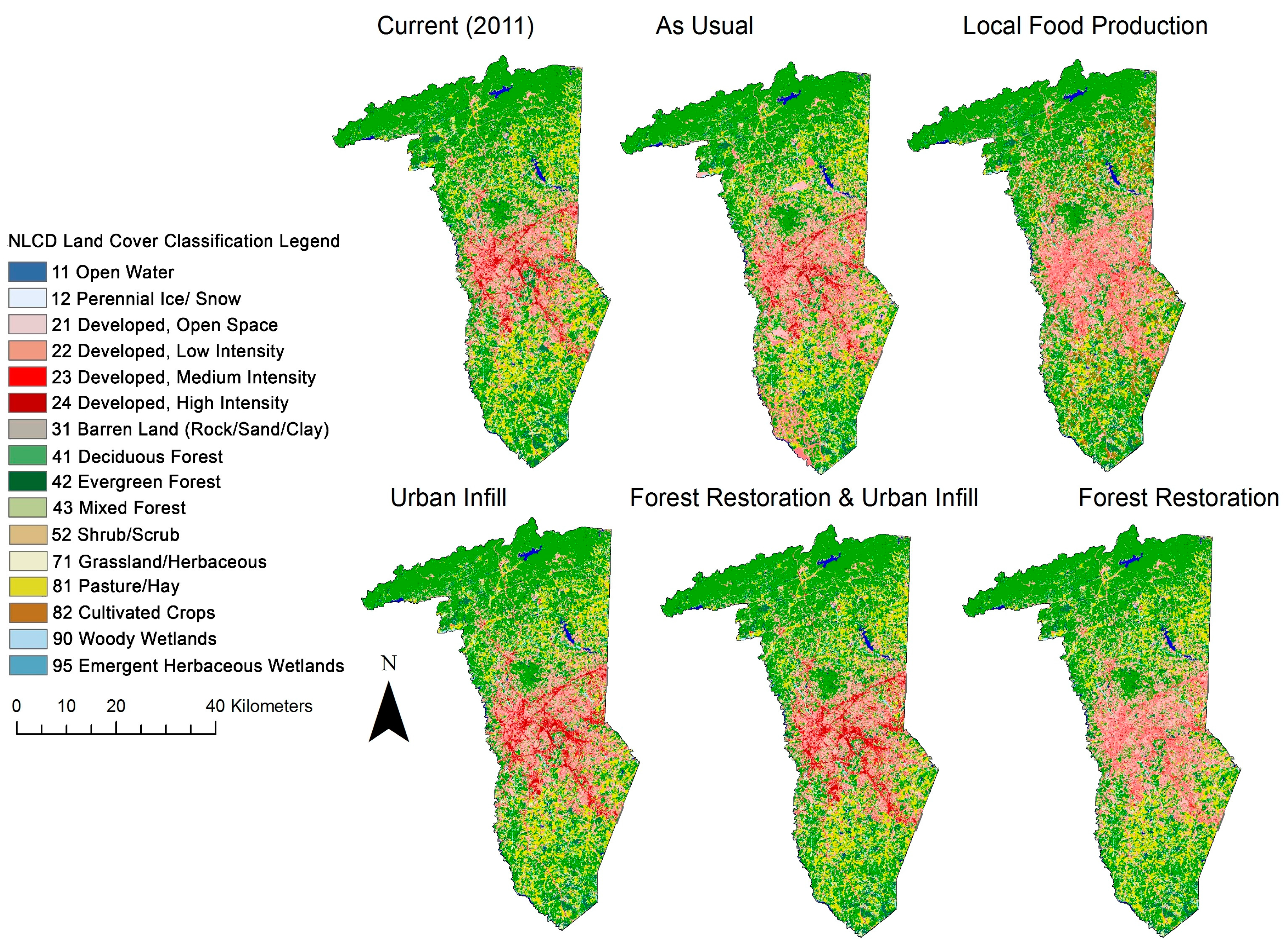
Land use changed with each scenario (Figure 2, Figure 3). In the as usual scenario, developed open and low density LULC types had the largest increase, resulting in a decline in grassland, shrubland and deciduous and evergreen forests to account for the urban sprawl. In the food production scenario, cropland increased to 7444% of its current spread to account for the county providing its own food supply. For urban infill, developed open areas were changed to developed-low and developed-medium density were transitioned into developed-high areas while natural habitat LULC types were preserved. The forest urban infill scenario saw a 5% increase in forest cover, with a slight decrease in shrub and grasslands. This scenario also converted developed open areas into developed low density and developed medium density into developed high density areas. The forest restoration scenario reduced the amount of developed high density LULC type and shrubland to restore and increase forests by 5%. Urban growth occurred in the developed open and low LULC types in this scenario.
3.2. Habitat Quality
3.2.1. Forest Interior Species
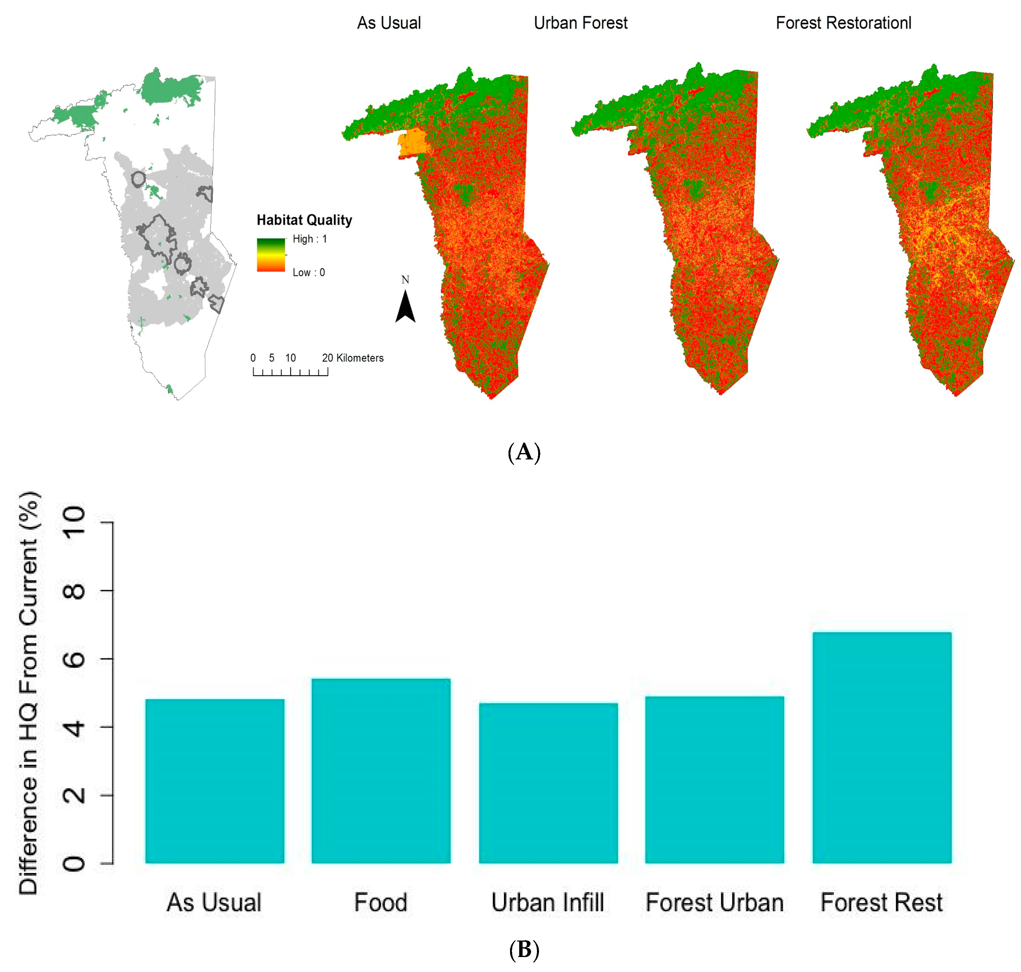
For every scenario, average habitat quality for forest interior species was between 70% and 80%. The average habitat quality for forest interior species in the current landscape was 70%. The greatest difference in habitat quality between the current and future scenarios was in the forest restoration scenario, in which the average habitat quality increased to 77%, making it the best scenario for forest interior species (Figure 4). The urban infill scenario resulted in the lowest habitat quality increase, resulting in an average habitat quality of 75%. Forest interior species had the most similar habitat quality changes across all of the scenarios, perhaps indicating their resilience within the Greenville County landscape.
3.2.2. Pine Specialist Species
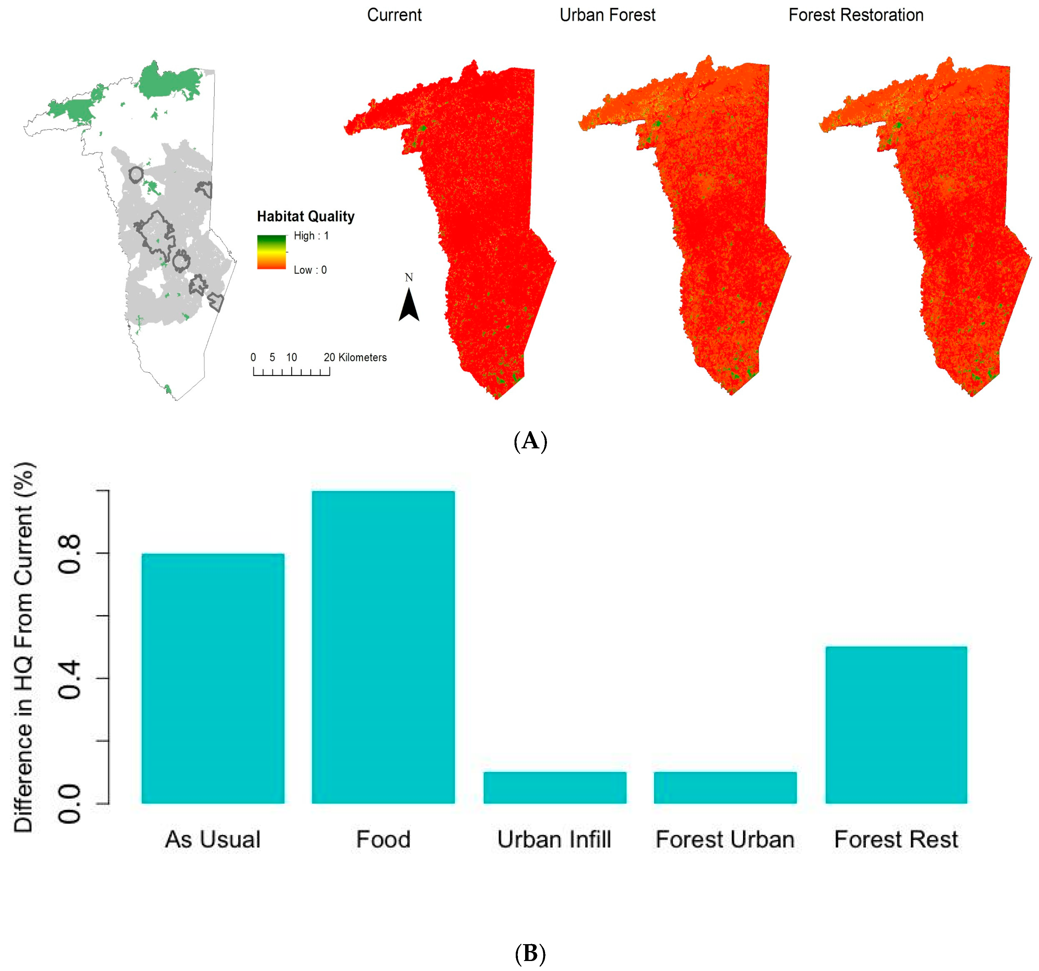
For all scenarios, average habitat qualities for pine specialist species were between 30% and 40%. The current landscape average habitat quality for pine specialists was 37%. The greatest difference in average habitat quality between current and future scenarios was in the food production scenario (Figure 5), though the magnitude of change was less than the interior forest cover habitat. This scenario increased the average habitat quality to 38%. The worst scenarios for pine specialist species success were the urban infill and forest urban infill scenarios; however, those scenarios saw an increase in average habitat quality from the current state by 0.1%.
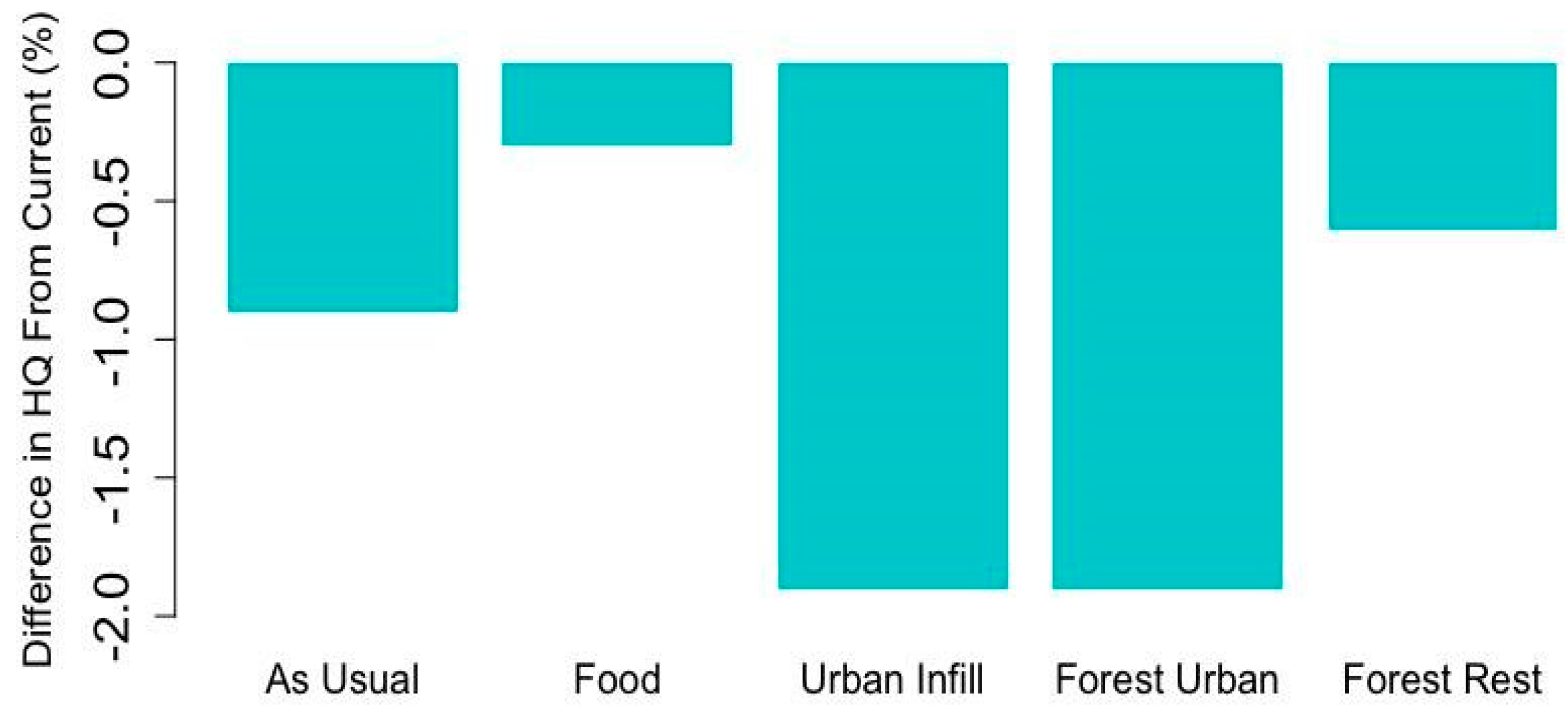
3.2.3. Shrub Specialist Species
Across all scenarios, shrub specialist species had average habitat qualities between 40% and 50%. The average habitat quality in the current landscape for shrub specialists was 43%. All scenarios resulted in a decrease in habitat quality for shrub specialist species (Figure 6). The greatest difference in habitat quality between current and future scenarios occurred in the urban infill and forest urban infill scenarios, which both had an average habitat quality of 41%. The best scenario for shrub specialist habitat was the food production scenario, in which the average habitat quality was 43%.
3.3. Carbon Sequestration
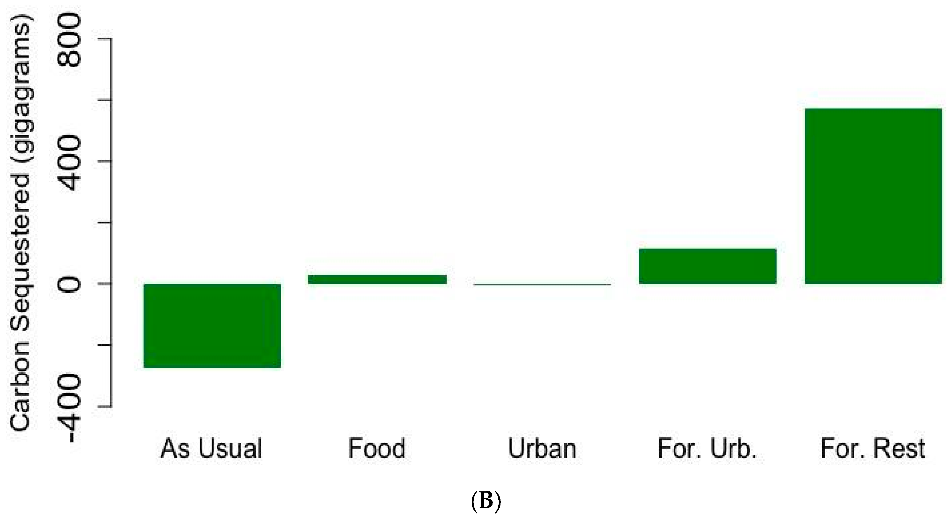
Three scenarios had increases in carbon sequestration; the forest restoration scenario, the forest urban infill scenario and the food production scenario (Figure 7). The forest restoration scenario had the greatest amount of carbon sequestration (571,576 Mg). The forest urban infill scenario had the second most carbon sequestration (113,796 Mg); however, sequestration is substantially less than that of the forest restoration scenario. The food production scenario had a slight increase in sequestration compared to the current carbon sequestration within the landscape (30,829 Mg). The other two scenarios saw a decrease in sequestration from that of the current landscape. Compared to the current state of carbon sequestration in Greenville County, the urban infill scenario had a slight decrease in sequestration (−2928 Mg), but this decrease is not significantly lower than the current carbon sequestration in Greenville County. The as usual scenario saw the largest decrease in carbon sequestration in Greenville County (−274,550 Mg). The economic value of the carbon sequestration follows the trends of the sequestered carbon.
3.4. Recreation
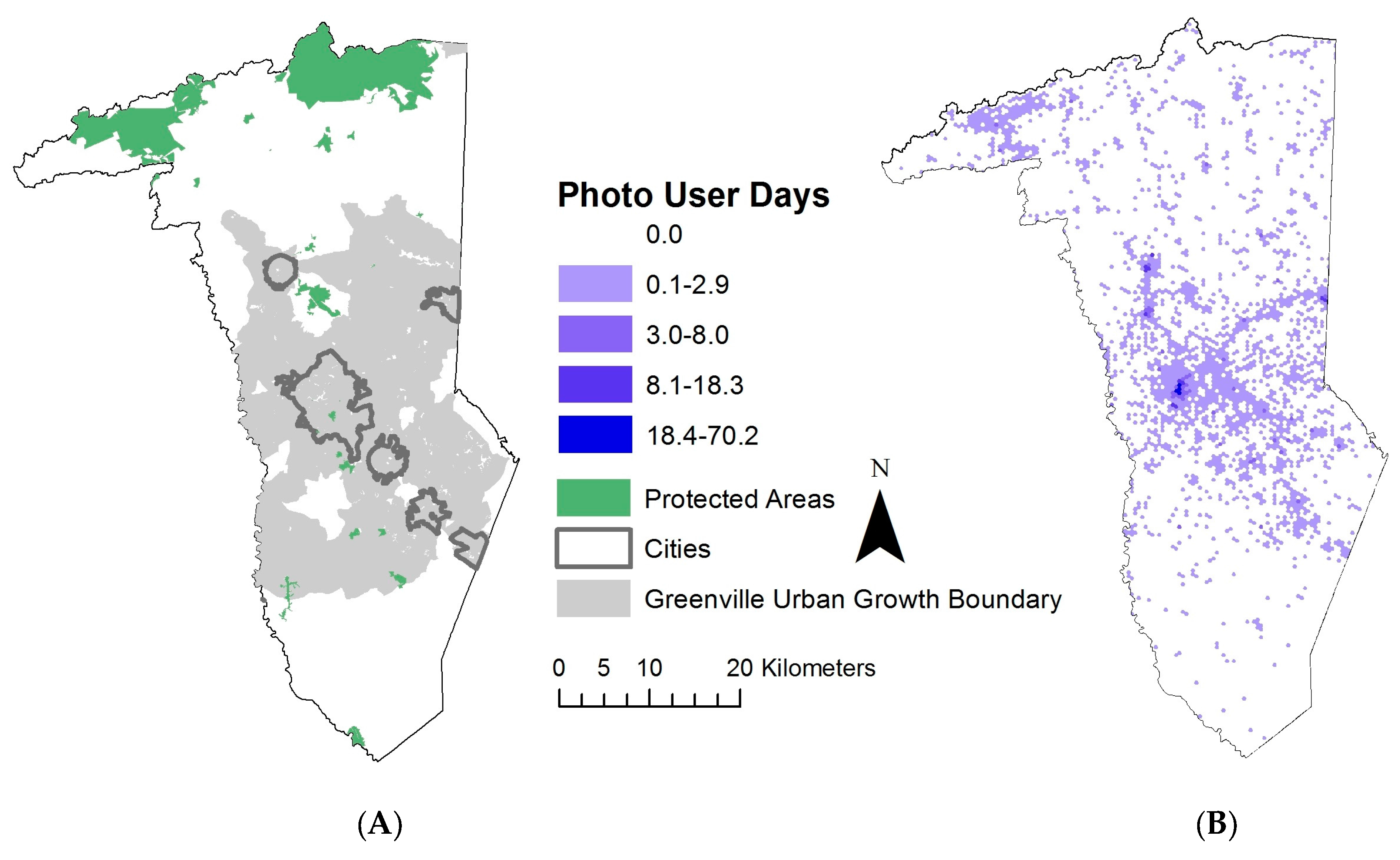
Areas of recreation in Greenville County occur mostly in settlements and populated forests (Figure 8). The proxy of photograph user days indicated that the most recreation for Greenville County is located in higher density urban areas; medium-level recreation occurs in protected areas across the northern county line (Figure 8).
3.5. Bundling Ecosystem Services and Overlapping Protected Areas
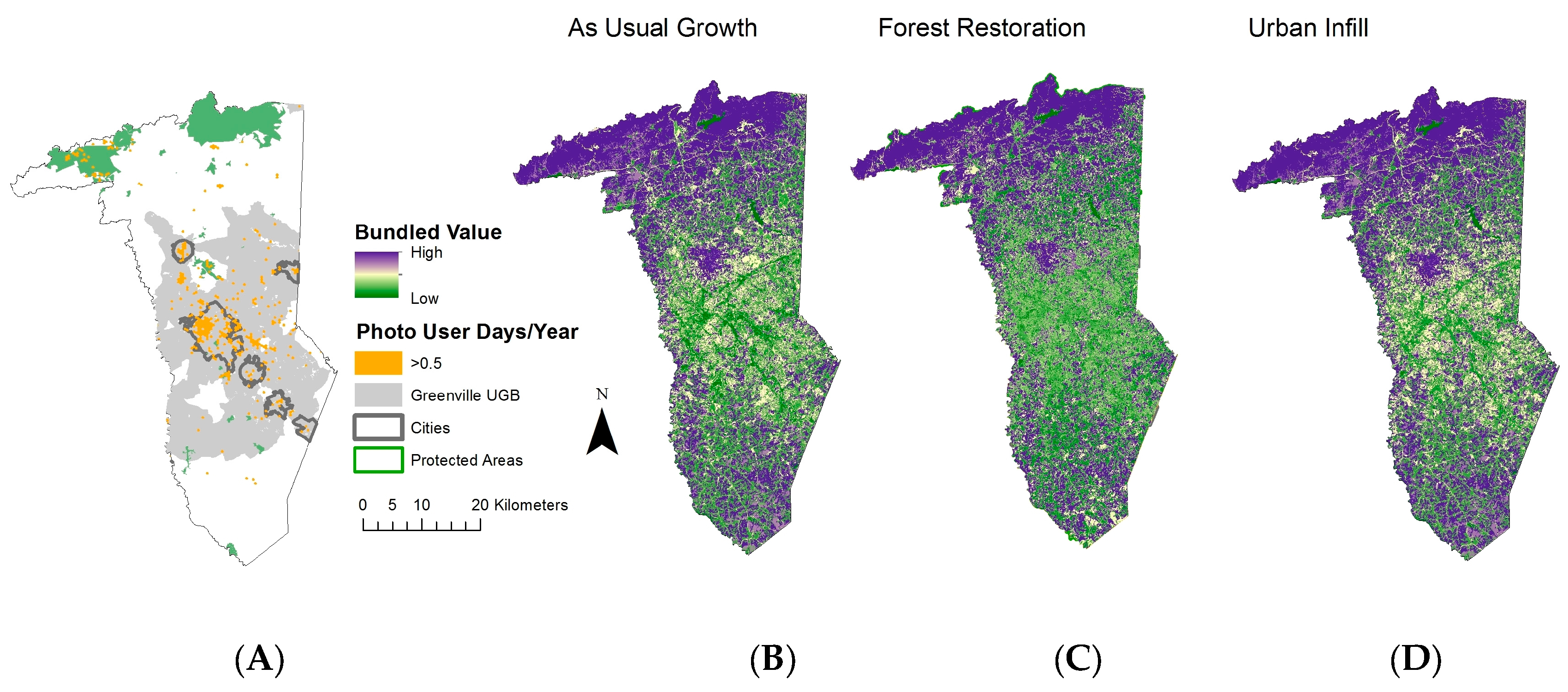
Evaluation of the spatial overlap between ecosystem services and biodiversity provides one way to look for multiple benefits in a scenario or for a unit of land (Figure 9). The overlap in forest interior species habitat quality, carbon stored and recreation demonstrates the value of currently protected areas in the northeast portion of the county, but also of the urban green space within the city. The areas of highest ecosystem service bundling are located in large, continuous tracts of protected areas. Areas of medium to high bundled value are located within and adjacent to protected areas. The smaller, fragmented protected areas, especially in the urban center of the county, contain medium to low levels of bundled benefits.
4. Discussion
The benefits of evaluating and visualizing different futures before they occur are clear (Naidoo et al., 2006 [11], Nelson et al., 2008 [15], Polasky et al., 2008 [30]). However, future scenarios need to realistically portray possible social and ecological conditions. Our conversations with stakeholders initially focused on the historical land use types for the region (Quinn et al., 2015 [37], Quinn and Wood, 2017 [14]), specifically the temperate deciduous forest biome that recovered following largescale abandonment of agricultural lands. Using the anthrome paradigm (Ellis et al., 2010 [1]) in our scenario development improved the narrative and evaluation of outcomes; in particular, it encouraged the participation of a diverse group of actors, identified multiple opportunities and challenges and resulted in scenarios that reflected a realistic context for future change. This latter benefit is most tangibly seen in the narrative of the scenarios. Given that scenarios are as much qualitative narratives as they are a summary of data, framing is essential. In this case study, rather than seeking to return to an arbitrary baseline of natural land cover (i.e., biome), an anthrome-based narrative framed LULC changes to reflect the social and ecological realities (Liu et al., 2007 [7]). Ultimately, by engaging multiple stakeholders in this process, we evaluated tradeoffs representing the social outlook of those residing on the landscape and the priorities policy makers in the region. Comparison of the spatial variation in the impacts of each scenario on different measures of biodiversity and ecosystem services allows stakeholders to see which of the conservation goals are most viable to achieve given available resources (Kareiva et al., 2011 [17]).
Comparisons and overlaps of biodiversity measures and ecosystem services in potential futures are valuable when assessing conservation objectives. These data are valuable because they illustrate tradeoffs and conservation opportunities between alternative futures across multiple systems and scales. Forest conservation provides the most benefits from ecosystem services. However, restoring or even preserving forest cover is difficult while urban sprawl increases rapidly, as demonstrated through the LULC changes in the forest restoration and forest urban infill scenarios. Therefore, the other scenarios are important for highlighting realistic conservation opportunities within Greenville County. For example, although farmland was cited as an important aspect of Greenville County, it was very difficult to preserve when planning for the projected future in the food production scenario. Each species type we analyzed benefitted most from a different scenario. The as usual scenario could provide an opportunity for pine specialist species conservation, while the urban infill scenario suggests an opportunity for forest interior species conservation, and the food production scenario provides a conservation opportunity for shrub specialist species. However, when comparing across different species types, we face an ethical question about choosing one species over another, or one ecosystem service over another. Furthermore, the variation in carbon sequestration across the scenarios suggests a need to define a threshold of carbon sequestration within the landscape. Involving stakeholders in this process is essential to create and meet the conservation goals of a landscape for the future.
The narratives created in the scenarios forced conservation stakeholders to recognize and articulate more realistic conservation objectives. If scenarios were based on biomes, what is portrayed and discussed may not be realistic or even the most desirable. This reality became clearer when discussing the forest restoration scenario. For example, Greenville citizens have indicated a willingness to pay to increase forest cover in the county by 5% (Cozad et al. [41]), yet through the scenarios, we found that increasing forest cover is difficult when associated with populated woodlands and dense settlements. Despite ~50% forest cover in the county, only a small portion of this is without humans, which forces the realization that the forest in the region is unlikely to return to a recent historical baseline (Drummond and Loveland, 2010 [35]).
Indeed, the scenario and model analysis highlighted the importance of conservation in populated woodlands and dense settlements, such as forest patches in the urban or peri-urban center and in residential landscapes. Of the scenarios tested, the forest restoration scenario provides the most benefits. Yet, as a scenario most focused on potential vegetation, such a scenario limits the role of human systems in land use change (Liu et al., 2007 [7]), and this is perhaps of less value in decision making. Within the as usual scenario, higher levels of carbon sequestration are located adjacent to currently protected fragments within the urban center of Greenville County. The forest urban infill scenario resulted in many small forest areas with medium levels of carbon sequestration throughout the dense settlement. The as usual scenario suggested unexpected opportunity for pine specialist species conservation in urban regions. This unexpected conservation opportunity aligns with the trend in which pine and evergreen forests are expanding while urbanization continues in the larger region of the southeastern Piedmont and evidence that some pine wildlife communities can utilize urban forest patches (Wood and Quinn 2016 [36]). The urban infill scenario suggests an opportunity for forest interior species conservation. This conservation opportunity supports the data in which compact cities provide benefits for many species due to the positive impacts of a land sparing conservation strategy (Soga et al., 2014 [48]). Spatially bundling ecosystem services (i.e., Nelson et al., 2008 [15]) demonstrated how the landscape can achieve conservation goals for multiple ecosystem services simultaneously. Specifically, the models suggest that an increased amount of protected areas within the urban center of Greenville County could benefit multiple ecosystem services, no matter which scenario occurs. Given that much of the forest in the region is populated and residential forest, planning efforts are going to be need to be taken in conjunction with local private landowners (Quinn and Wood, 2017 [14]). Comparing between similar anthromes in different parts of the world can help align targets to opportunities, realities or unexpected threats. As noted above, many of the largest urban centers are embedded within/surrounded by populated woodlands. Thus, with more scenarios built around anthromes, locally relevant case studies can be aggregated and compared more across other scenario planning projects.
5. Conclusions
Anthromes have emerged as an important concept in framing conservation opportunities and challenges (Martin et al., 2014 [9]). Leveraging their utility to conservation scenario planning improves the process and outcomes. Individually, these data are valuable; however, their worth increases when coupled across systems and scales identifying alternative futures that enhance regional conservation and planning efforts within anthromes. These findings highlight conservation opportunities in dense settlements and populated woodlands, with a particular focus on the large tracts of populated forests in northern Greenville County, as well as the fragmented urban center of Greenville County. The spatial arrangement and overlap of ecosystem services and protected areas identifies distinct conservation opportunities within different scenarios while also emphasizing areas that provide important conservation opportunities across all alternative futures. Working within the anthrome paradigm allows researchers, planners and stakeholders to better understand the tradeoffs and synergies at landscape scales by spatially overlapping conservation and human system goals, which is essential for achieving benefits for humans and natural systems in complex, rapidly urbanizing areas (Kareiva and Marvier, 2012 [8]).
Acknowledgments
Funding was provided by Furman University and The Shi Center for Sustainability. We thank the editor and two reviewers for helpful comments on the manuscript.
Author Contributions
D.M.G. and J.E.Q. conceived of and designed the research. D.M.G. performed the scenarios and models. D.M.G. and J.E.Q. analyzed the data. D.M.G. and J.E.Q. wrote the paper.
Conflicts of Interest
The authors declare no conflict of interest.
References
- Ellis, E.C.; Klein Goldewijk, K.; Siebert, S.; Lightman, D.; Ramankutty, N. Anthropogenic transformation of the biomes, 1700 to 2000. Glob. Ecol. Biogeogr. 2010, 19, 589–606. [Google Scholar] [CrossRef]
- Ellis, E.C.; Ramankutty, N. Putting people in the map: Anthropogenic biomes of the world. Front. Ecol. Environ. 2008, 6, 439–447. [Google Scholar] [CrossRef]
- Hansen, M.C.; Potapov, P.V.; Moore, R.; Hancher, M.; Turubanova, S.A.; Tyukavina, A.; Thau, D.; Stehman, S.V.; Goetz, S.J.; Loveland, T.R.; et al. High-resolution global maps of 21st-Century forest cover change. Science 2013, 342, 850–853. [Google Scholar] [CrossRef] [PubMed]
- Costanza, R.; d’Arge, R.; de Groot, R.; Farberk, S.; Grasso, M.; Hannon, B.; Limburg, K.; Naeem, S.; O’Neill, R.V.; Paruelo, J.; et al. The value of the world’s ecosystem services and natural capital. Nature 1997, 387, 253–260. [Google Scholar] [CrossRef]
- United Nations, Department of Economic and Social Affairs, Population Division. World Urbanization Prospects: The 2014 Revision, Highlights; (ST/ESA/SER.A/352); United Nations, Department of Economic and Social Affairs: New York, NY, USA, 2014. [Google Scholar]
- Butchart, S.H.; Walpole, M.; Collen, B.; Van Strien, A.; Scharlemann, J.P.; Almond, R.E.; Baillie, J.E.; Bomhard, B.; Brown, C.; Bruno, J.; et al. Global biodiversity: Indicators of recent declines. Science 2010, 328, 1164–1168. [Google Scholar] [CrossRef] [PubMed]
- Liu, J.; Dietz, T.; Carpenter, S.R.; Alberti, M.; Folke, C.; Moran, E.; Pell, A.N.; Deadman, P.; Kratz, T.; Lubchenco, J.; et al. Complexity of coupled human and natural systems. Science 2007, 317, 1513–1516. [Google Scholar] [CrossRef] [PubMed]
- Kareiva, P.; Marvier, M. What is conservation science? BioScience 2012, 62, 962–969. [Google Scholar]
- Martin, L.J.; Quinn, J.E.; Ellis, E.C.; Shaw, M.R.; Dorning, M.A.; Hallett, L.M.; Heller, N.E.; Hobbs, R.J.; Kraft, C.E.; Law, E.; et al. Conservation opportunities across the world’s anthromes. Divers. Distrib. 2014, 20, 745–755. [Google Scholar] [CrossRef]
- Golladay, S.W.; Martin, K.L.; Vose, J.M.; Wear, D.N.; Covich, A.P.; Hobbs, R.J.; Klepzig, K.D.; Likens, G.E.; Naiman, R.J.; Shearer, A.W. Achievable future conditions as a framework for guiding forest conservation and management. For. Ecol. Manag. 2016, 360, 80–96. [Google Scholar] [CrossRef]
- Naidoo, R.; Balmford, A.; Ferraro, P.J.; Polasky, S.; Ricketts, T.H.; Rouget, M. Integrating economic costs into conservation planning. Trends Ecol. Evol. 2006, 21, 681–687. [Google Scholar] [CrossRef] [PubMed]
- Deng, J.S.; Wang, K.; Hong, Y.; Qi, J.G. Spatio-temporal dynamics and evolution of land use change and landscape pattern in response to rapid urbanization. Landsc. Urban Plan. 2009, 92, 187–198. [Google Scholar] [CrossRef]
- Sandifer, P.A.; Sutton-Grier, A.E.; Ward, B.P. Exploring connections among nature, biodiversity, ecosystem services, and human health and well-being: Opportunities to enhance health and biodiversity conservation. Ecosyst. Serv. 2015, 12, 1–15. [Google Scholar] [CrossRef]
- Quinn, J.E.; Wood, J.M. Application of a coupled human natural system framework to organize and frame challenges and opportunities for biodiversity conservation on private lands. Ecol. Soc. 2017, 22, 39. [Google Scholar] [CrossRef]
- Nelson, E.; Polasky, S.; Lewis, D.J.; Plantinga, A.J.; Lonsdorf, E.; White, D.; Bael, D.; Lawler, J.J. Efficiency of incentives to jointly increase carbon sequestration and species conservation on a landscape. Proc. Natl. Acad. Sci. USA 2008, 105, 9471–9476. [Google Scholar] [CrossRef] [PubMed]
- De Groot, R.S.; Alkemade, R.; Braat, L.; Hein, L.; Willemen, L. Challenges in integrating the concept of ecosystem services and values in landscape planning, management and decision making. Ecol. Complex. 2010, 7, 260–272. [Google Scholar] [CrossRef]
- Kareiva, P.; Tallis, H.; Ricketts, T.H.; Daily, G.C.; Polasky, S. Natural Capital: Theory and Practice of Mapping Ecosystem Services; OUP Oxford: Oxford, UK, 2011. [Google Scholar]
- Sanon, S.; Hein, T.; Douven, W.; Winkler, P. Quantifying ecosystem service trade-offs: The case of an urban floodplain in Vienna, Austria. J. Environ. Manag. 2012, 111, 159–172. [Google Scholar] [CrossRef] [PubMed]
- Nelson, E.; Mendoza, G.; Regetz, J.; Polasky, S.; Tallis, H.; Cameron, D.; Chan, K.M.; Daily, G.C.; Goldstein, J.; Kareiva, P.M.; et al. Modeling multiple ecosystem services, biodiversity conservation, commodity production, and tradeoffs at landscape scales. Front. Ecol. Environ. 2009, 7, 4–11. [Google Scholar] [CrossRef]
- Goldstein, J.H.; Caldarone, G.; Duarte, T.K.; Ennaanay, D.; Hannahs, N.; Mendoza, G.; Polasky, S.; Wolny, S.; Daily, G.C. Integrating ecosystem-service tradeoffs into land-use decisions. Proc. Natl. Acad. Sci. USA 2012, 109, 7565–7670. [Google Scholar] [CrossRef] [PubMed]
- Lambin, E.F.; Turner, B.L.; Geist, H.J.; Agbola, S.B.; Angelsen, A.; Bruce, J.W.; Coomes, O.T.; Dirzo, R.; Fischer, G.; Folke, C.; et al. The causes of land-use and land-cover change: Moving beyond the myths. Glob. Environ. Chang. 2001, 11, 261–269. [Google Scholar] [CrossRef]
- Contreras-Hermosilla, A. The Underlying Causes of Forest Decline; CIFOR occasional paper 30; CIFOR: Bogor, Indonesia, 2000. [Google Scholar]
- Boit, A.; Sakschewski, B.; Boysen, L.; Cano-Crespo, A.; Clement, J.; Garcia-alaniz, N.; Kok, K.; Kolb, M.; Langerwisch, F.; Rammig, A.; et al. Large-scale impact of climate change vs. land-use change on future biome shifts in Latin America. Glob. Chang. Biol. 2016, 22, 3689–3701. [Google Scholar] [CrossRef] [PubMed]
- Uden, D.R.; Allen, C.R.; Mitchell, R.B.; McCoy, T.D.; Guan, Q. Predicted avian responses to bioenergy development scenarios in an intensive agricultural landscape. GCB Bioenergy 2015, 7, 717–726. [Google Scholar] [CrossRef]
- Grimm, N.B.; Foster, D.; Groffman, P.; Grove, J.M.; Hopkinson, C.S.; Nadelhoffer, K.J.; Pataki, D.E.; Peters, D.P. The changing landscape: Ecosystem responses to urbanization and pollution across climatic and societal gradients. Front. Ecol. Environ. 2008, 6, 264–272. [Google Scholar] [CrossRef]
- Castro, A.J.; Verburg, P.H.; Martín-López, B.; Garcia-Llorente, M.; Cabello, J.; Vaughn, C.C.; López, E. Ecosystem service trade-offs from supply to social demand: A landscape-scale spatial analysis. Landsc. Urban Plan. 2014, 132, 102–110. [Google Scholar] [CrossRef]
- Lauf, S.; Haase, D.; Kleinschmit, B. Linkages between ecosystem services provisioning, urban growth and shrinkage—A modeling approach assessing ecosystem service trade-offs. Ecol. Indic. 2014, 42, 73–94. [Google Scholar] [CrossRef]
- Marzluff, J.M. Worldwide urbanization and its effects on birds. In Avian Ecology and Conservation in an Urbanizing World; Springer: New York, USA, 2001; pp. 1–19. [Google Scholar]
- Quinn, J.E.; Johnson, R.J.; Brandle, J.R. Identifying opportunities for conservation embedded in cropland anthromes. Landsc. Ecol. 2014, 29, 1811–1819. [Google Scholar] [CrossRef]
- Polasky, S.; Nelson, E.; Camm, J.; Csuti, B.; Fackler, P.; Lonsdorf, E.; Montgomery, C.; White, D.; Arthur, J.; Garber-Yonts, B.; et al. Where to put things? Spatial land management to sustain biodiversity and economic returns. Biol. Conserv. 2008, 141, 1505–1524. [Google Scholar] [CrossRef]
- Urban Land Institute South Carolina. Upstate Reality Check. 2017. Available online: http://southcarolina.uli.org/upstate-reality-check/ (accessed on 1 May 2017).
- Terando, A.J.; Costanza, J.; Belyea, C.; Dunn, R.R.; McKerrow, A.; Collazo, J.A. The southern megalopolis: Using the past to predict the future of urban sprawl in the Southeast US. PLoS ONE 2014, 9, e102261. [Google Scholar] [CrossRef] [PubMed]
- Andersen, C.B.; Donovan, R.K.; Quinn, J.E. Human Appropriation of Net Primary Production (HANPP) in an agriculturally-dominated watershed, southeastern USA. Land 2015, 4, 513–540. [Google Scholar] [CrossRef]
- Veldkamp, A.; Lambin, E.F. Predicting land-use change. Agric. Ecosyst. Environ. 2001, 85, 1–6. [Google Scholar] [CrossRef]
- Drummond, M.A.; Loveland, T.R. Land-use pressure and a transition to forest-cover loss in the eastern united states. Bioscience 2010, 60, 286–298. [Google Scholar] [CrossRef]
- Wood, J.; Quinn, J.E. Local and landscape metrics identify opportunities for conserving cavity-nesting birds in a rapidly urbanizing ecoregion. J. Urban Ecol. 2016, 2, juw003. [Google Scholar] [CrossRef]
- Quinn, C.; Quinn, J.E.; Halfacre, A. Digging Deeper: A Case Study of Farmer Conceptualization of Ecosystem Services in the American South. Environ. Manag. 2015, 56, 802–813. [Google Scholar] [CrossRef] [PubMed]
- McDonnell, M.J.; Pickett, S.T. Ecosystem structure and function along urban-rural gradients: An unexploited opportunity for ecology. Ecology 1990, 71, 1232–1237. [Google Scholar] [CrossRef]
- Chiesura, A. The role of urban parks for the sustainable city. Landsc. Urban Plan. 2003, 68, 129–138. [Google Scholar] [CrossRef]
- Steiner, F. Opportunities for urban ecology in community and regional planning. J. Urban Ecol. 2016, 2, 1–2. [Google Scholar] [CrossRef]
- Cozad, M.; Warnken, J.; Quinn, J.E. Willingness to pay for forest conservation in rapidly urbanizing ecosystems: A case study in Upstate South Carolina. 2017; in preparation. [Google Scholar]
- Ernstes, R.; Quinn, J.E. Variation in bird vocalizations across a gradient of traffic noise as a measure of an altered urban soundscape. Cities Environ. 2016, 8, 7. [Google Scholar]
- Polasky, S.; Nelson, E.; Pennington, D.; Johnson, K.A. The impact of land-use change on ecosystem services, biodiversity and returns to landowners: A case study in the state of Minnesota. Environ. Resour. Econ. 2011, 48, 219–242. [Google Scholar] [CrossRef]
- Bagstad, K.J.; Semmens, D.J.; Waage, S.; Winthrop, R. A comparative assessment of decision-support tools for ecosystem services quantification and valuation. Ecosyst. Serv. 2013, 5, 27–39. [Google Scholar] [CrossRef]
- Peters, C.J.; Wilkins, J.L.; Fick, G.W. Testing a complete-diet model for estimating the land resource requirements of food consumption and agricultural carrying capacity: The New York State example. Renew. Agric. Food Syst. 2007, 22, 145–153. [Google Scholar] [CrossRef]
- Zumkehr, A.; Campbell, J.E. The potential for local croplands to meet US food demand. Front. Ecol. Environ. 2015, 13, 244–248. [Google Scholar] [CrossRef]
- Wood, S.A.; Guerry, A.D.; Silver, J.M.; Lacayo, M. Using social media to quantify nature-based tourism and recreation. Sci. Rep. 2013, 3, 2976. [Google Scholar] [CrossRef] [PubMed]
- Soga, M.; Yamaura, Y.; Koike, S.; Gaston, K.J. Land sharing vs. land sparing: Does the compact city reconcile urban development and biodiversity conservation? J. Appl. Ecol. 2014, 51, 1378–1386. [Google Scholar] [CrossRef]
Figure 1.
The location of Greenville County (white outline) in relation to the southeastern Piedmont anthromes in the United States, with the additional note of urban centers Atlanta, Georgia, and Charlotte, North Carolina. (Ellis et al., 2010 [1]).
Figure 1.
The location of Greenville County (white outline) in relation to the southeastern Piedmont anthromes in the United States, with the additional note of urban centers Atlanta, Georgia, and Charlotte, North Carolina. (Ellis et al., 2010 [1]).

Figure 2.
Scenario maps. The spatial arrangement of LULC types in Greenville County for the current LULC from 2011 and for all 2035 scenarios.
Figure 2.
Scenario maps. The spatial arrangement of LULC types in Greenville County for the current LULC from 2011 and for all 2035 scenarios.

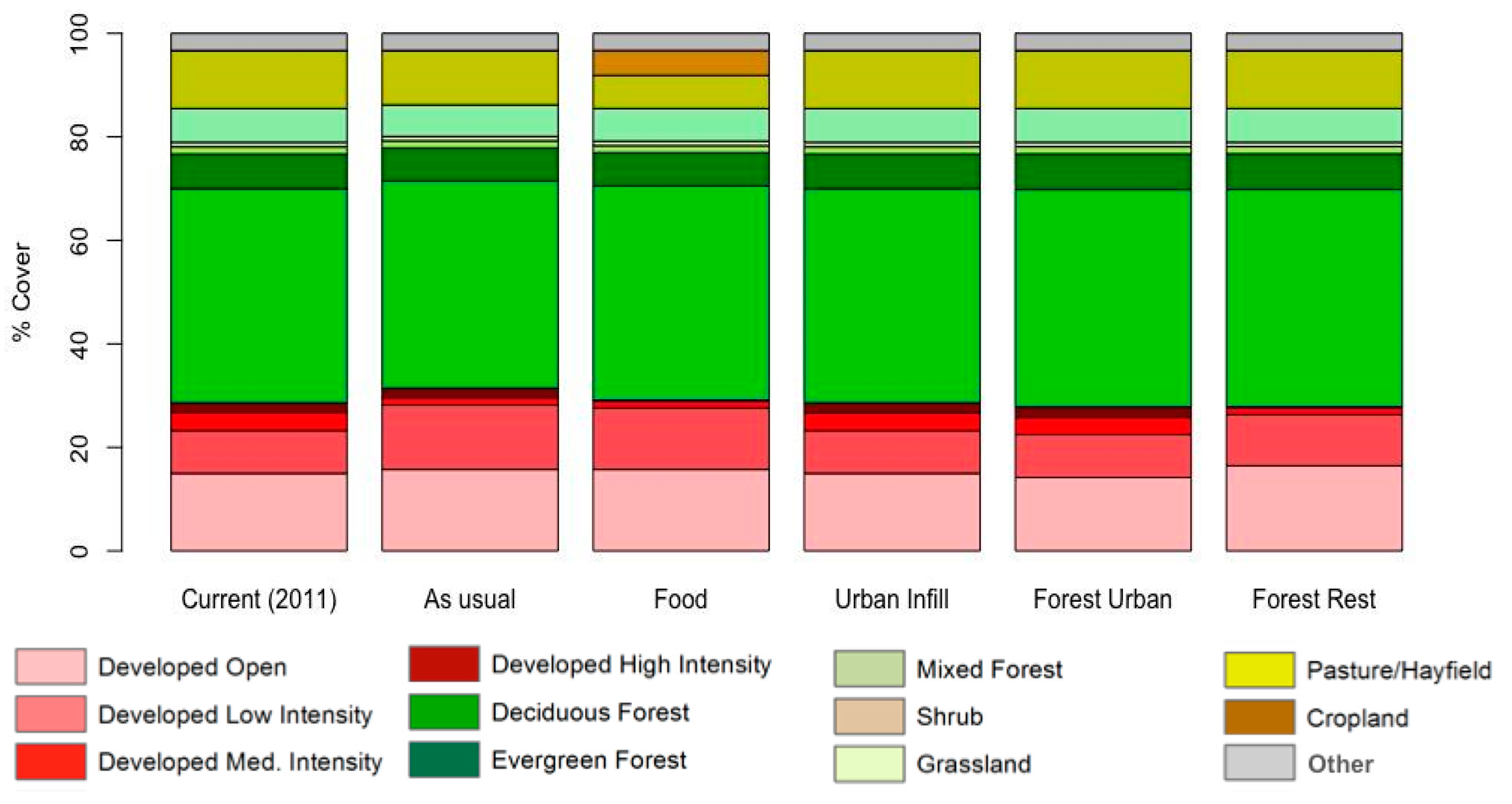
Figure 3.
Relative LULC in each scenario. The relative cover of each LULC type within each scenario for Greenville County in 2035, with a comparison to the current (2011) LULC, showing the magnitude of LULC change in each scenario relative to other LULC types.
Figure 3.
Relative LULC in each scenario. The relative cover of each LULC type within each scenario for Greenville County in 2035, with a comparison to the current (2011) LULC, showing the magnitude of LULC change in each scenario relative to other LULC types.

Figure 4.
(A) Difference between the current average habitat quality and scenario average habitat quality for forest interior species. (B) All scenarios resulted in an increase in average habitat quality from the current landscape.
Figure 4.
(A) Difference between the current average habitat quality and scenario average habitat quality for forest interior species. (B) All scenarios resulted in an increase in average habitat quality from the current landscape.

Figure 5.
(A) Difference between the current average habitat quality and scenario average habitat quality for pine specialist species. (B) All scenarios showed an increase in average habitat quality for pine specialist species from that of the current landscape.
Figure 5.
(A) Difference between the current average habitat quality and scenario average habitat quality for pine specialist species. (B) All scenarios showed an increase in average habitat quality for pine specialist species from that of the current landscape.

Figure 6.
Difference between the current average habitat quality and scenario average habitat quality for shrub specialist species. All scenarios resulted in a decrease in average habitat quality from that of the current landscape.
Figure 6.
Difference between the current average habitat quality and scenario average habitat quality for shrub specialist species. All scenarios resulted in a decrease in average habitat quality from that of the current landscape.

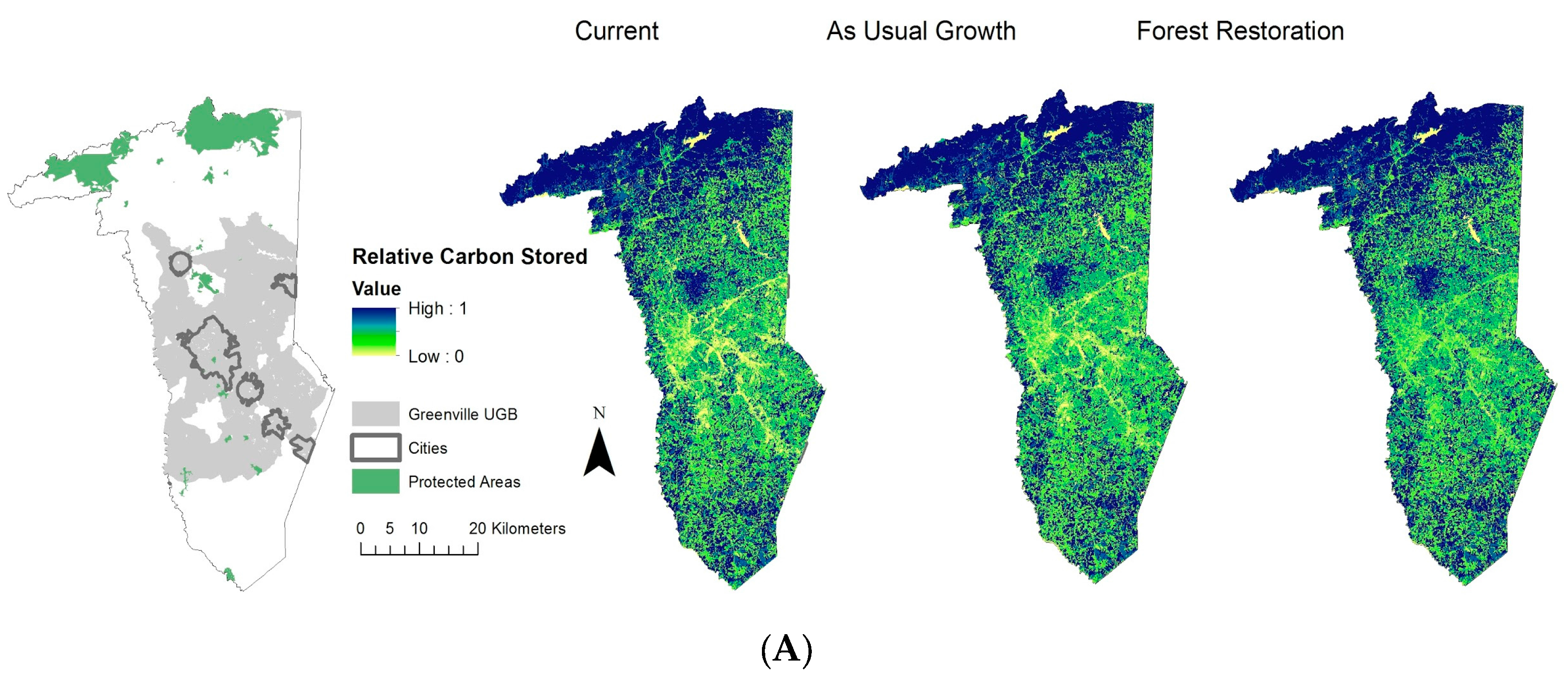
Figure 7.
(A) Spatial variation in carbon stored across current and two possible future land use patterns. (B) Carbon sequestered in each scenario. The amount of carbon, in gigagrams, that would be sequestered by the landscape in each 2035 scenario: as usual, food production (Food), urban infill (Urban), forest urban infill (For. Urb.) and forest restoration (For. Rest).


Figure 8.
Recreation on the landscape. The spatial overlap of urban growth expectations and protected areas (A) and recreation (B). Photo user days are used as a proxy for recreation.
Figure 8.
Recreation on the landscape. The spatial overlap of urban growth expectations and protected areas (A) and recreation (B). Photo user days are used as a proxy for recreation.

Figure 9.
Overlap of photo user days and protected area (A) with bundled forest interior habitat quality and carbon in the as usual (B), forest restoration (C), and urban infill (D) scenarios in Greenville County, SC, USA.
Figure 9.
Overlap of photo user days and protected area (A) with bundled forest interior habitat quality and carbon in the as usual (B), forest restoration (C), and urban infill (D) scenarios in Greenville County, SC, USA.


Table 1.
Brief descriptions of land use/land cover scenarios. The explanation of the focus for each of the five projected land use and land cover scenarios for Greenville County, SC, in 2035. All scenarios account for a 100% increase in population in the county.
Table 1.
Brief descriptions of land use/land cover scenarios. The explanation of the focus for each of the five projected land use and land cover scenarios for Greenville County, SC, in 2035. All scenarios account for a 100% increase in population in the county.
| Scenario | Description |
|---|---|
| As Usual | The expected landscape if current urban sprawl trends continue as the county experience 100% population growth |
| Food Production | The projected landscape if we prioritize providing local food as the population has a 100% increase |
| Urban Infill | The planned landscape in which focusing on increasing urban density and infilling urban areas accounts for the 100% increase in population |
| Forest Urban Infill | The plan for increasing urban density to account for the projected population growth while increasing forested areas by 5% |
| Forest Restoration | The projected landscape that focuses on forest restoration to increase forested areas by 5% while allowing for a 100% increase in population |
Table 2.
Comparing land use/land cover in each scenario. The percentage of land use/land cover for current Greenville County, SC, as well as each scenario for Greenville County. The amount of water, barren, woody wetlands and herbaceous wetlands land use and land cover types were held constant across all scenarios.
| Water | Developed Open | Developed Low | Developed Medium | Developed High | Barren | Deciduous Forest | Evergreen Forest | Mixed Forest | Shrub | Grassland | Pasture | Cropland | Woody Wetlands | Herbaceous Wetlands | |
|---|---|---|---|---|---|---|---|---|---|---|---|---|---|---|---|
| Current (2011) | 1.00% | 14.98% | 8.29% | 3.55% | 1.78% | 0.40% | 41.40% | 6.67% | 1.40% | 0.89% | 6.53% | 11.15% | 0.06% | 1.87% | 0.03% |
| As Usual | 1.00% | 15.73% | 12.44% | 1.42% | 1.85% | 0.40% | 40.06% | 6.36% | 1.38% | 0.85% | 6.10% | 10.45% | 0.06% | 1.87% | 0.03% |
| Food Production | 1.00% | 15.73% | 11.87% | 1.42% | 0.09% | 0.40% | 41.40% | 6.43% | 1.36% | 0.87% | 6.31% | 6.41% | 4.81% | 1.87% | 0.03% |
| Urban Infill | 1.00% | 14.98% | 8.29% | 3.37% | 1.96% | 0.40% | 41.40% | 6.67% | 1.40% | 0.89% | 6.53% | 11.15% | 0.06% | 1.87% | 0.03% |
| Forest Urban Infill | 1.00% | 14.18% | 8.29% | 3.37% | 1.96% | 0.40% | 42.02% | 6.87% | 1.40% | 0.86% | 6.53% | 11.15% | 0.06% | 1.87% | 0.03% |
| Forest Restoration | 1.00% | 16.44% | 9.87% | 1.42% | 0.09% | 0.40% | 42.02% | 6.87% | 1.40% | 0.84% | 6.53% | 11.15% | 0.06% | 1.87% | 0.03% |
© 2017 by the authors. Licensee MDPI, Basel, Switzerland. This article is an open access article distributed under the terms and conditions of the Creative Commons Attribution (CC BY) license (http://creativecommons.org/licenses/by/4.0/).
Share and Cite
MDPI and ACS Style
Gibson, D.M.; Quinn, J.E. Application of Anthromes to Frame Scenario Planning for Landscape-Scale Conservation Decision Making. Land 2017, 6, 33. https://0-doi-org.brum.beds.ac.uk/10.3390/land6020033
AMA Style
Gibson DM, Quinn JE. Application of Anthromes to Frame Scenario Planning for Landscape-Scale Conservation Decision Making. Land. 2017; 6(2):33. https://0-doi-org.brum.beds.ac.uk/10.3390/land6020033
Chicago/Turabian StyleGibson, Dainee M., and John E. Quinn. 2017. "Application of Anthromes to Frame Scenario Planning for Landscape-Scale Conservation Decision Making" Land 6, no. 2: 33. https://0-doi-org.brum.beds.ac.uk/10.3390/land6020033
Note that from the first issue of 2016, this journal uses article numbers instead of page numbers. See further details here.