Estimation of the Spatiotemporal Patterns of Vegetation and Associated Ecosystem Services in a Bornean Montane Zone Using Three Shifting-Cultivation Scenarios

Abstract

Tropical countries are now facing increasing global pressure to conserve tropical forests, while having to maintain cultivated lands (particularly shifting cultivation) for the subsistence of local people. To accomplish the effective conservation of tropical forests in harmony with subsistence shifting cultivation, we evaluated the influence of shifting cultivation on ecosystem services (i.e., biodiversity and carbon stock) at a landscape level based on three land-use scenarios. The study focus was the upland area between the Kinabalu Park and the Crocker Range Park in Sabah, northern Borneo, where local people conduct shifting cultivation for their subsistence. In this area, vegetation patches of various stages of secondary succession admix with shifting-cultivation lands. An earlier study in the same site depicted significant relationships between the stand ages of vegetation patches (which form a sere of secondary succession after the abandonment of cultivated land) and the above-ground biomass (i.e., carbon stock) and species composition of the stands. We incorporated these significant relationships to a stand-age estimation algorithm that had been developed earlier. We first mapped current (as of 2010) spatial patterns of the above-ground biomass and plant-community composition for the whole landscape. Subsequently, we simulated the spatiotemporal patterns of the above-ground biomass and plant-community distribution using three land-use scenarios: (1) reducing the area of shifting cultivation by one half and protecting the rest of the area; (2) shortening the minimum fallow period from 7 to 4 years while maintaining the same area of cultivation; and (3) elongating the minimum fallow period from 7 to 10 years while maintaining the same area of cultivation. Results indicated that land use based on scenario 2 could increase the carbon stock while maintaining the cultivation area. Our methods were effective in mapping the structure and composition of highly dynamic forests at a landscape level, and at predicting the future patterns of important ecosystem services based on land-use scenarios.

1. Introduction

Shifting cultivation is a widespread form of land use in tropical regions, and has formed the basis of livelihoods and customs for centuries [1,2,3,4]. This traditional land use still remains central to the livelihoods, culture and food security of millions of people in tropical regions [5]. At the same time, however, shifting cultivation is a direct cause of deforestation, and considered a prominent source of carbon emissions [6,7] with associated biodiversity loss [8,9,10,11]. Tropical countries are, therefore, facing increasing pressure to conserve tropical forests while having to maintain cultivated lands (particularly shifting cultivation) for the subsistence of local people.

Where there is a long history of shifting cultivation, patches of successional vegetation intermix with old-growth forests and form spatiotemporally heterogeneous landscape patterns [12]. Such spatiotemporally dynamic and heterogeneous landscapes occur widely across many tropical countries [13,14]. Land patterns that consist of successional vegetation and old-growth matrixes (hereafter referred to as land mosaics) are now regarded as an important provider of ecosystem services in contemporary landscapes dominated by humans [15,16].

In order to design appropriate conservation policies for land mosaics, two different approaches were proposed: a ‘land-sparing’ agricultural approach and a ‘land-sharing’ agricultural approach [15,17,18]. A land-sparing approach suggests reducing the area of farmland by emphasizing high-yielding, more intensive production, and trading reduced ecosystem services within the farmland for the retention of ecosystem services in protected areas. A land-sharing approach integrates food production with the protection of ecosystem services in the same land area [17]. An important question is whether there is a sharp trade-off between the ecosystem services derived from strictly protected areas and the agricultural production from farmlands in land mosaics, or if both ecosystem services and agricultural production can be enhanced in land mosaics. Both approaches can potentially cause a sharp trade-off or the reconciliation of ecosystem service and agriculture. However, such analyses are surprisingly lacking for tropical regions, partly due to the fact that land mosaics are too dynamic to investigate [19]. Therefore, developing an appropriate methodology to investigate the spatiotemporal relationships between ecosystem services and farmlands (particularly shifting cultivation) in land mosaics is needed in order to design appropriate conservation policies [20].

To evaluate the spatiotemporal relationships between ecosystem services and farmlands, the integration of ecological understanding and remote-sensing data is crucial [21]. Fujiki et al. [22] found that plant-species composition (richness) and above-ground biomass (a surrogate of carbon stock) demonstrated explicit temporal patterns after the abandonment of slash-and-burn cultivation in the same Bornean upland area where we conducted this study. In this case, the time elapsed after slash and burn is the most important determinant of species composition and biomass in the secondary-vegetation patches of this site. Provided that stand ages (i.e., time elapsed after slash and burn) of vegetation patches are identified by remote sensing, species composition and biomass can be mapped at a landscape level, and even their spatiotemporal patterns can be simulated as a function of time with appropriate land-use scenarios. Fujiki et al. [12] developed an algorithm to estimate stand ages of vegetation patches based on remote-sensing data in the same area as the study of Fujiki et al. [22].

Therefore, the objective of our study was to evaluate the spatiotemporal patterns of ecosystem services associated with vegetation succession in the shifting cultivation area by extrapolating the explicit temporal patterns of species composition and biomass derived by Fujiki et al. [22] into the stand-age algorithm developed by Fujiki et al. [12]. Firstly, we evaluated the spatial patterns of plant-species composition and biomass of vegetation patches as of 2010, when high-resolution satellite data were taken. Subsequently, we simulated the future patterns of above-ground biomass using three land-use scenarios and compared the results with the extant patterns as of 2010. Lastly, we discussed how to synergize the conservation of ecosystem services with shifting cultivation and suggested appropriate conservation policies by comparing the scenarios.

2. Materials and Methods

2.1. Study Site and Field Survey

Our study site is a gap in an upland area between the Kinabalu Park and the Crocker Range Park in Sabah, northern Borneo. We chose this area because it is located within forests that have some of the richest collections of vascular species in the world [23], while at the same time very small patches of fragmented forest are scattered throughout the area. The gap between the two parks is approximately 10 km in length and has long been inhabited by indigenous people who practice shifting cultivation for subsistence. The government of Sabah has set forth a policy to enhance ecological linkages between the two parks by increasing secondary forests as stepping stones in the gap area, and considers REDD+ (Reducing Emissions from Deforestation and Forest Degradation-Plus) as an important mechanism to incentivize local people [24]. REDD+ is a financial mechanism to encourage carbon increments (i.e., increased forests) compared with the baseline (i.e., the current practice of shifting cultivation). Therefore, the evaluation and prediction of carbon stock in the gap area are of critical concern to the local government.

One family slashes and burns patches of young- to old-growth forests, cultivates upland rice for the first year, and abandons the land for fallow [22]. In between the two parks, there is another local forest reserve (Tenompok Forest Reserve) with pristine vegetation, which is strictly protected from any subsistence use by local regulations. Local people, therefore, conduct traditional shifting cultivation outside of the parks and the reserve. The central point of the study site is at 5°58′ N and 116°29′ E. The altitude of the area ranges from 300 m to 1700 m. The total annual rainfall and mean annual temperature are approximately 2000–2500 mm and 15–24 °C, respectively. The geology of this area consists of tertiary sedimentary rock of the West Crocker Formation [24]. The original vegetation of this area is the lower montane tropical rainforest dominated by the families Fagaceae, Myrtaceae and Lauraceae [25,26].

Fujiki et al. [22] conducted a field survey for 2 months in the same site in August 2012 and August 2013. Details of the field survey were described in Fujiki et al. [22]. In short, they randomly selected a total of 27 stands in this area in order to establish inventory plots. Twenty-five stands were selected to represent the ages of a few to 55 years after shifting cultivation. Two stands were selected in an old-growth forest more than 100 years after slash and burn. The altitudes of these stands varied between 900 m and 1400 m asl. A plot was placed in each stand. Descriptions of stand age, altitude, above-ground biomass (AGB) and dominant species in each of the 27 vegetation stands are shown in Table S1 (cited from Fujiki et al. [22]). We used the same stands for the following analyses to estimate AGB and plant-species composition.

We conducted additional field surveys in the same site in April and September 2014 to validate the accuracy of subsequent AGB estimation. The details of the procedure were almost the same as the field survey of Fujiki et al. [22]. Twelve 400-m² circular plots were randomly established in the area to represent the ages of 4 to 26 years after shifting cultivation (Table S2). The altitudes of these plots varied between 1000 m and 1400 m asl. The diameter at breast heigh (dbh) of all trees (dbh ≥ 5 cm) was measured in each of the main plots while trees with 5 cm > dbh ≥ 1 cm were measured in a sub-plot (25 m²). Global positioning system (GPS) data were collected during the field surveys at the center of a plot with calibration for at least one hour in each plot. We used these additional plots only for validating the results of AGB estimation in the following remote-sensing analysis.

2.2. Field Data Analysis

Fujiki et al. [22] estimated AGB and analyzed the species composition of plant communities with a multivariate DCA (detrended correspondence analysis) using the same 27 stands. To estimate the AGB of trees with dbh ≥ 1 cm, they used an empirical allometric relationship reported for tropical secondary forests after shifting cultivation in Sarawak, Malaysia [27], with a similar climate and flora as our site:

AGB (kg m⁻²) = 0.0829 dbh ^2.43

(1)

The AGB of trees with dbh ≥ 5 cm in the additional 12 plots were also calculated using the same allometric equation.

Fujiki et al. [22] conducted a multivariate DCA to elucidate the gradients in both species composition and their environmental controls using CANOCO Version 4.5 [28] software. DCA was run using the default options, detrending by segments and non-linear rescaling. Fujiki et al. [22] used the relative abundance of each species based on coverage for all inventoried species per stand. They conducted these analyses using 25 stands (age ≤ 55 years) excluding the two oldest stands (age > 100 years), because the exact ages of these stands could not be identified and their species composition was very different from the other stands. The results of DCA are shown by a biplot of stands and species in Figure S1 (cited from Fujiki et al. [22]). They also categorized the same 25 stands into five groups using TWINSPAN. The first group was categorized as herbaceous community with an average height of 3.3 m. The second group was a shrub community with an average height of 7.5 m. The third group was categorized as an upper montane short-forest community above 1100 m asl with an average height of 19.8 m. The fourth group was categorized as a lower montane short-forest community below 1100 m asl. The last group was categorized as an (old-fallow) forest community with the canopy height of 23.0 m. We used these categories to interpret the results of the estimation of plant-community composition in the following remote-sensing analysis.

3. Remote-Sensing Analysis

3.1. Extrapolation Procedure of Above-Ground Biomass (AGB) and Community Composition

Orthorectified WorldView-2 multi spectral images (22 June 2010), Landsat-5 TM (1 March 1988; 14 June 1991; 22 August 1993; 1 February 1995; 14 June 1997; 8 September 1999; 17 June 2004; 7 June 2006; 28 April 2009) and Landsat-7 ETM+ (19 March 2002) images were used in this study. Details of the pre-processing of the images were described in Fujiki et al. [12]. Briefly, raw digital numbers of each image were converted into surface-reflectance values using the 6S (Second Simulation of a Satellite Signal in the Solar Spectrum) atmospheric correction model [29]. Topographically induced local variations in angular viewing geometry were reduced using the method described by [30]. All clouds and cloud-shadows in each image were removed by unsupervised classification with ISODATA and visual inspection. ERDAS Imagine (ver.11.0; ERDAS Inc., Norcross, GA, USA) and ArcGIS 9.3 (ESRI, Redlands, CA, USA) were used during the entire pre-processing.

Details of the process of stand-age estimation can be referred to Fujiki et al. [12]. In brief, we extracted temporal information (i.e., stand ages after shifting cultivation) from a change-detection analysis with Landsat time-series images and superimposed the stand ages on the segments classified by an object-based analysis using WorldView-2. The basic units of object-based analysis were image segments, each of which was composed of spectrally coherent pixel clusters based on homogeneity criteria. Each segment identified by the object-based analysis reflected a land parcel of shifting cultivation where secondary succession proceeded to a variety of stages. Stand ages from change-detection analysis were regarded as a response variable and object-based metrics of each segment as independent variables in order to develop regression models that explained stand ages. Before establishing the regression models, the WorldView-2 segments were divided into some broad vegetation types (i.e., non-vegetated, 1–7 years, 7–50 years, over 50 years, and rubber plantations) with a decision-tree method, using a normalized difference vegetation index (NDVI) threshold and linear discriminant analyses (LDA). Although each of the 1–7-year and 7–50-year vegetation types was subdivided into several age categories in the original study of Fujiki et al. [12], stand age was estimated as a continuous value ranging from 0 to 50 years in this current study using the same multiple regression models as in Fujiki et al. [12]. We used ERDAS Imagine (ver. 11.0; ERDAS Inc., Atlanta, GA, USA) for the change-detection analysis, and eCognition Developer (ver. 8.7; Definiens AG, Munich, Germany) for the object-based analyses.

Subsequently, we used the regression model between stand age and AGB developed by Fujiki et al. [22] (Figure S2a) to estimate AGB at a landscape level, combined with the age-estimation algorithm described above. Fujiki et al. [22] found that species composition was primarily patterned by stand ages (as sorted along axis 1 of the DCA) and, secondly, by stand altitudes (as sorted along axis 2). We, therefore, derived correlation models by regressing DCA axis 1 scores as a response variable with stand ages as an independent variable (Figure S2b), and by regressing DCA axis 2 scores as a response variable with stand altitudes as an independent variable (Figure S2c). The models used in this study are as follows:

GB (Mg ha⁻¹) = 8.38 + 2.53 SA (R² = 0.88, p < 0.001)

(2)

DCA axis 1 = 1.568 + 1.255 ln (SA) (R² = 0.69, p < 0.001)

(3)

DCA axis 2 = 7.250 − 0.005 ALT (R² = 0.44, p < 0.001)

(4)

where SA denotes stand age, and ALT denotes altitude. DCA axis 1 and axis 2 are the first and the second axes that explained the greatest and the second greatest variation of plant-species composition in the DCA analysis, respectively.

The AGB model was extrapolated to the stand-age map for the vegetation types between the ages of 1–50 years old. For fallow vegetation older than 50 years, the mean AGB of the two old-fallow stands was uniformly assigned. The DCA axis 1 and axis 2 scores were respectively extrapolated to the stand-age map and an elevation map. The elevation map was derived from the Shuttle Radar Topography Mission (SRTM-1, 30-m mesh). We removed the areas above 1400 m and below 900 m elevation from the analysis for plant-community composition, because the altitude of inventory plots ranged from 900 m to 1400 m. The estimated DCA axes’ scores were shown as a red/green composite image. Green colors were used to express the gradient of DCA axis 1 scores and red colors were used to express the gradient of DCA axis 2 scores. A base map was produced to reflect the condition as of 22 June 2010, the date when the WorldView-2 multispectral image was taken. Therefore, extrapolated AGB and DCA axis scores reflect the ground patterns as of 22 June 2010.

The accuracy of the AGB estimation map was assessed and expressed as a root mean square error (RMSE) determined by comparison between observed vs. estimated AGB values. To determine the RMSE, we used field-observed AGB values of the 12 validation plots and corresponding AGB values estimated from WorldView-2 images. In contrast to the acquisition date of the WorldView-2 in 2010, the validation plots were established in 2014. Therefore, the AGB values of the validation plots were adjusted to the year 2010 for their intermediate growth, using the AGB-stand age (SA) model described above. An estimated AGB within the 11.3 m-radius (400 m²) from the center of each validation plot was compared with the value actually observed. Then, the relationship between estimated and observed values of AGB was derived as a linear regression.

3.2. Simulations Using Land-Use Scenarios

The total newly cultivated area as of 2010 was 635 ha and the number of newly cultivated parcels was 2660. The current minimum and maximum fallow period was approximately 7 years and 20 years, respectively (estimated from the histogram of the current vegetation pattern [12]). The maximum fallow period was defined as a maximum stand age of vegetation which local people selected to slash and burn.

In order to elucidate the influences of different practices of shifting cultivation on the future vegetation and carbon stock, we simulated the vegetation dynamics based on three scenarios, and then evaluated the associated AGB changes. We adopted the following scenarios: (1) ‘reduced-cultivation’ scenario; (2) ‘shorter-fallow’ scenario; and (3) ‘longer-fallow’ scenario. These scenarios were arbitrarily set and all were intended to enhance future carbon stock to meet the government’s strategy. In scenario 1, we assumed that the annual cultivation area would be reduced by one half and the minimum fallow period of shifting cultivation would be kept constant (i.e., 7 years). In scenario 2, the annual cultivation area would be kept constant but, instead, the minimum fallow period of shifting cultivation would be shortened from 7 to 4 years. In scenario 3, the minimum fallow period of shifting cultivation would be elongated from 7 to 10 years while the annual cultivation area would be kept constant. The shorter fallow period in scenario 2 was expected to promote forest succession at a landscape level, with cultivated areas being confined to a more limited area, because shifting cultivation with a shorter fallow period tended to use the same area more intensively and, thus, the rest of the area would escape from slash and burn. The longer fallow in scenario 3 was also expected to promote forest succession and increase total AGB at a stand level without a reduction of cultivation area.

Based on the three scenarios, we simulated the dynamics of vegetation patterns and AGB for 10 years from 2010 to 2020, and the results derived were compared with the baseline (i.e., 2010). In the simulations, we assumed that one segment identified by the object-based analysis represented one parcel of vegetation patch (or one parcel of cultivated land), and controlled the number of annually cultivated segments each with a mean area of 3100 m². The actual segment area varies according to the parcel selected. Therefore, total cultivated area actually slightly varies over the years. Each segment has a stand age as an integer, estimated from the age-estimation algorithm. We controlled two parameters in each simulation: the total number of annually cultivated segments (i.e., annual cultivation area), and the min–max fallow period (i.e., the min–max stand age of the segments which local people select to slash and burn). The min–max fallow period was set as 7–20 years in scenario 1, as 4–20 years in scenario 2, and as 10–40 years in scenario 3. As will be shown, the land available for shifting cultivation actually was not enough in scenario 3 because all of the 10–20-year segments were converted into vegetation younger than 10 years with 4 iterations of the simulation. Therefore, the maximum fallow period of 40 years was used exceptionally in scenario 3 (i.e., local people could cultivate stands as old as 40 years).

We estimated the stand age of all segments of the whole study area at one-year intervals from 2010 to 2020 in each simulation. In each year, 1330 segments for scenario 1 (half of the annually cultivated segments in the current state) and 2660 segments for scenarios 2 and 3 were randomly selected from the segments with stand ages between a given min–max fallow period in each simulation. We converted the stand ages of the selected segments into 0 (i.e., the occurrence of annual shifting cultivation), and added 1 to the stand age of the rest of the segments (i.e., annual increment in stand age). This step was iterated for 10 times in each scenario. Subsequently, the AGB stock in 2020 was calculated from the segment ages derived from each simulation. The histograms of segment age and AGB stock in 2020 were compared with those of the current state (as of 2010).

4. Results

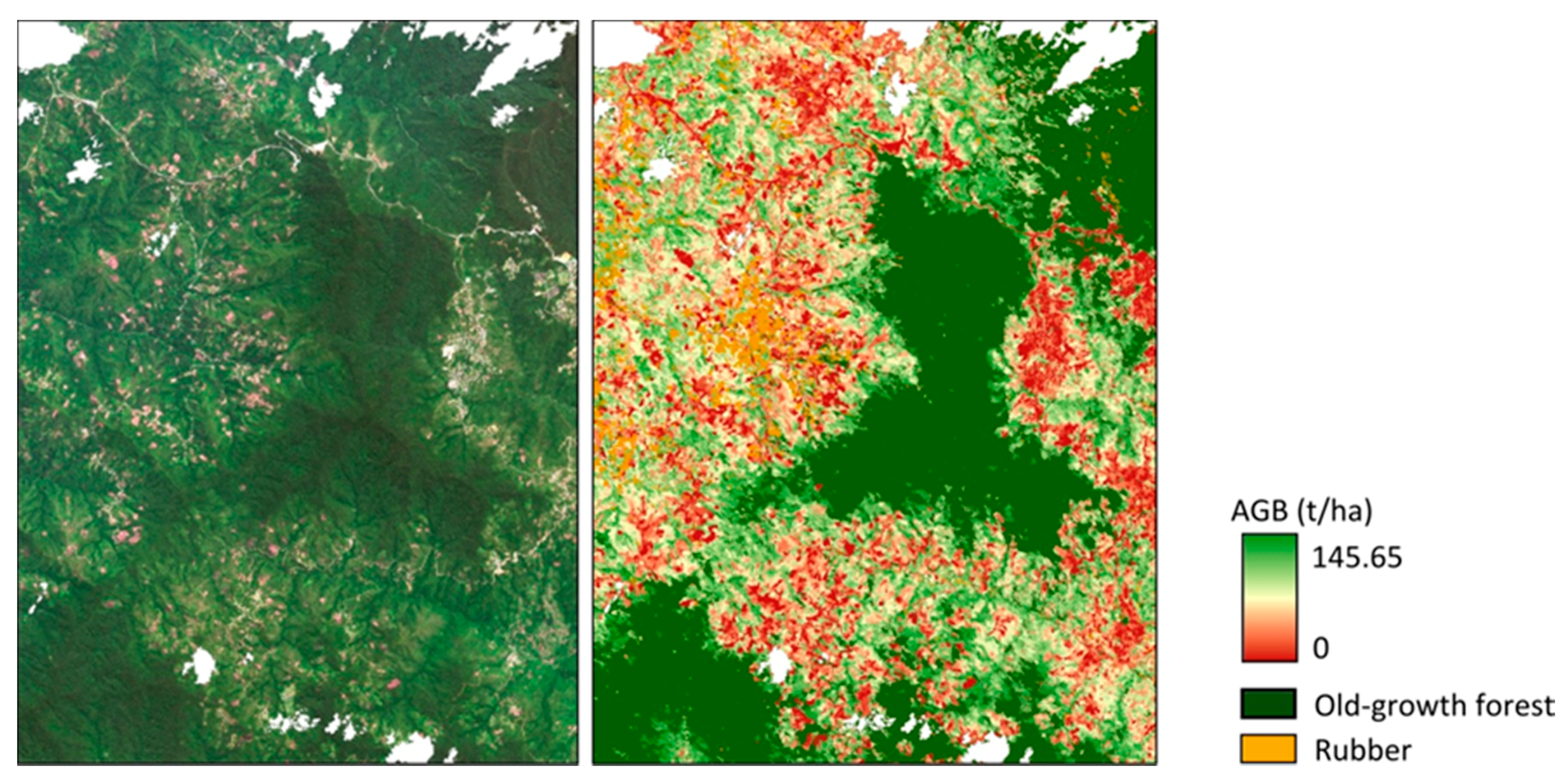
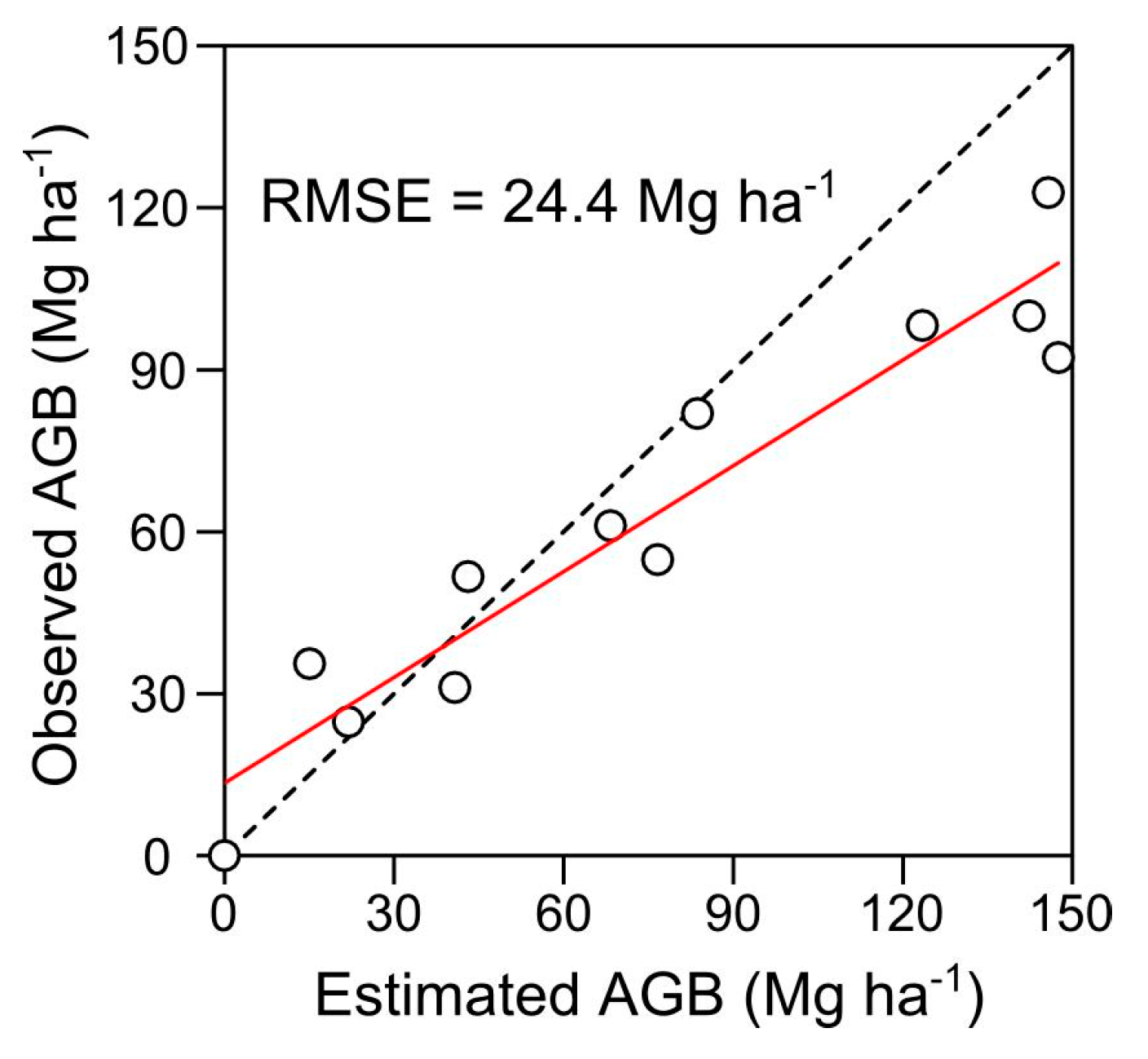
4.1. AGB Map and Plant-Community Composition Map

The results of the AGB estimation as of 2010 are shown in Figure 1. Each pixel in the map contains an AGB value, and the color gradation from red to green indicates a gradient of AGB values from low to high. Vegetation with a medium AGB is densely distributed around the edge of the strictly protected areas (dark green color). On the other hand, lower-AGB vegetation is sparsely distributed over the whole area. Total AGB stock in the total area (15,000 ha) is 1,530,000 Mg (equivalent to 104 Mg ha⁻¹) and total AGB stock in the successional vegetation (1 to 50-year-old vegetation including cultivated area; 9300 ha) is 363,000 Mg (equivalent to 39 Mg ha⁻¹). The relationships between the estimated and observed AGB of 12 validation plots are shown in Figure 2. The RMSE between the estimated and observed AGB was 24.4 Mg ha⁻¹. However, the deviation of the regression line from the 1:1 line suggested an increasing overestimation of AGB in older vegetation.

The results of the estimation of plant-community composition are shown in Figure 3. Each pixel in the map shows both DCA axis 1 and DCA axis 2 scores as a red/green spectral composite. Green-color spectrum is used for DCA axis 1 scores and red-color spectrum is used for DCA axis 2 scores. The spectral matrix shows the gradation of the change of composition. The spectral matrix was divided into five species-composition groups according to the category of Fujiki et al. [22]. Most of the area was covered with reddish colors which indicate the herbaceous community. A green color indicates the upper montane short forest community or old-fallow community, and these communities comprise the second largest land-cover component. The area of lower montane short-forest community (yellow color) was relatively small.

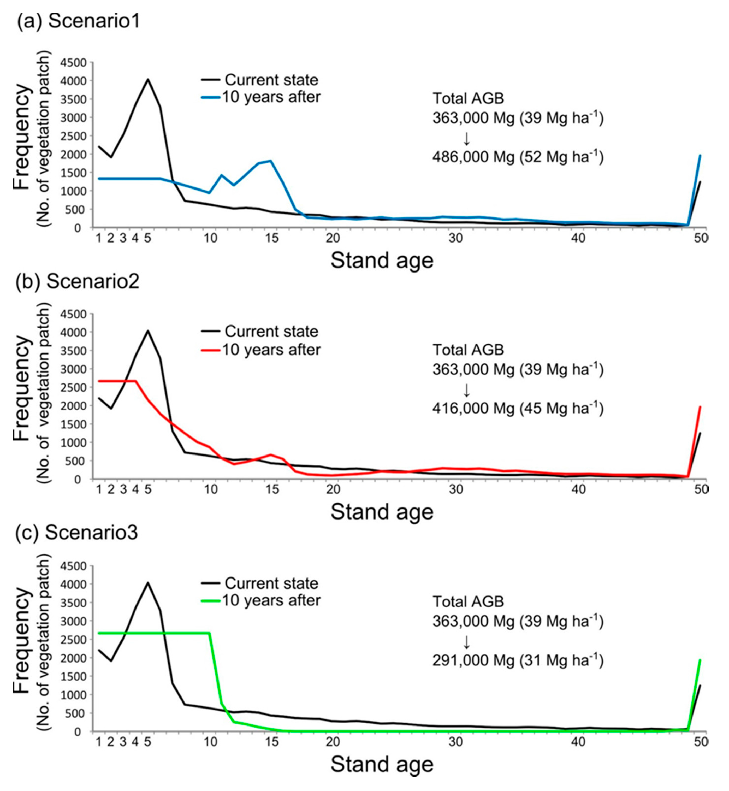
4.2. Numerical Simulation of Vegetation Patterns Based on Three Scenarios

The results of the simulations based on the three scenarios are shown in Figure 4 in terms of the frequency of vegetation patches (segments) per stand age. The black line indicates the vegetation pattern of the base map as of 2010. The blue line in Figure 4a is the vegetation pattern for the year 2020 based on scenario 1, where the cultivation area was reduced by one half for 10 years. Shifting-cultivation practices based on scenario 1 decreased the frequency of vegetation younger than 7 years and, instead, increased the frequency of vegetation with ages around 15 years. As a result, the total AGB in the successional vegetation (1–50-year-old vegetation including the cultivated area) was increased by 123,000 Mg (equivalent to 13.2 Mg ha⁻¹). Based on scenario 2, in which the minimum fallow period was reduced from 7 to 4 years, the frequency of both vegetation older than 7 years and younger than 4 years increased (Figure 4b). The total AGB in the successional vegetation was increased by 54,000 Mg (equivalent to 5.8 Mg ha⁻¹). On the other hand, the results of scenario 3 showed a different pattern. Based on scenario 3, in which the minimum fallow period was elongated from 7 to 10 years, the simulation could not be continued after four times of iteration with a maximum fallow period of 20 years, as explained earlier. This was because the number of 10–20-year segments became limited for selecting new cultivation areas as all of the 10–20-year segments were converted into vegetation younger than 10 years of age. Therefore, the simulation in Figure 4c was conducted in vegetation with ages up to 40 years. As a result, almost all of the vegetation younger than 40 years was disturbed and converted into vegetation younger than 10 years. The total AGB in the successional vegetation decreased by 72,000 Mg (equivalent to 7.7 Mg ha⁻¹) in this simulation.

5. Discussion

The stand-age map combined with the field-based AGB accumulation model was effective at estimating the AGB of land mosaics of shifting cultivation with secondary vegetation patches at a landscape level (RMSE: 24.4 Mg ha⁻¹). However, as shown in Figure 2, the AGB values were overestimated in the vegetation with higher AGB. This was probably because the identification of patch (segment) boundaries was not successfully undertaken, especially in the vegetation with higher AGB. The segments identified by the object-based analysis were sometimes mixed with the surrounding old-growth vegetation and erroneously regarded as extremely old. Our validation samples were included in such erroneously identified segments, which caused overestimation of vegetation with higher AGB. However, our AGB map is clearly useful for detecting the location and frequency of vegetation patches for a given AGB category.

The map of plant-community composition also clearly described the continuous gradients of the community shift in this area by a red/green spectral composite of both DCA axis 1 and DCA axis 2 scores. Most of the study area is covered with a herb community, upper montane short-forest community and old fallow community, whereas the area of lower montane short-forest community is smaller. Fischer et al. [14] suggested that conserving native vegetation alone will not protect ecosystem services, and that land mosaics should include patches of native vegetation, corridors and stepping stones between them, as well as buffers around the native vegetation. Our map can identify the areas of potentially high conservation values, or those with fewer ecosystem services where mitigation measures are required. Such information is useful for the management of corridors and stepping stones between protected areas, and building buffers around them.

The stand-age map can be used to predict future vegetation patterns with land-use scenarios. With both scenarios 1 and 2, it is possible to promote forest succession and increase total AGB at a landscape level. Scenario 1 (reducing the cultivation area) is the most effective scenario for promoting forest biomass accumulation and, probably, associated biodiversity. Scenario 2 (fallow reduced from 7 to 4 years, i.e., land-sharing) is also effective at promoting forest biomass accumulation in a landscape. This is because shifting cultivation with a shorter fallow period uses the same area repeatedly, and therefore the rest of the area escapes from slash and burn. Based on scenario 3 (a fallow period elongated from 7 to 10 years, i.e., land-sharing), local people cannot continue shifting cultivation within 4 years because the cultivation area has become saturated. Moreover, the total AGB stock in the successional vegetation is decreased.

Past ecological studies reported that shorter fallow periods under shifting cultivation lead to a decrease in species richness and diversity in situ [31,32,33,34]. However, our results suggest that shortening the fallow period of shifting cultivation results in promoting forest succession and increasing total AGB at a landscape level, provided that cultivation becomes intensified in a limited area. On the other hand, elongating the fallow period of shifting cultivation may promote broader deforestation at a landscape level. We suggest that forest dynamics in a whole landscape have to be taken into consideration for predicting the consequences of shifting cultivation.

Cultivation practices based on both scenarios 1 and 2 may not be able to maintain cultivation yields. With scenario 1, a reduced cultivation area will directly decrease crop yields if the average crop yield per area is constant. With scenario 2, a shorter fallow can also result in the reduction of crop yield, because intensive land use can decrease availability of soil nutrients such as phosphorus [22,35,36]. Such nutrient reductions and the associated decreases of crop yields indicate the difficulty in maintaining livelihood production with scenario 2. All three scenarios in this study, therefore, may not be able to reconcile livelihood production with forest conservation effectively.

In order to reconcile livelihood production with forest conservation, decreased crop yields have to be compensated for through appropriate mechanisms such as REDD+. This is an incentive-based policy mechanism often described as a payment-for-performance system, where people can receive financial support for carbon increments. Our method can provide quantitative information of the current carbon stock as well as expected carbon increments with improved land-use scenarios. Our method can also provide quantitative assessment of how/whether carbon increments can be reconciled with biodiversity conservation because maps derived from our method can elucidate both carbon and plant communities.

Once field-based models (i.e., the relationships of stand age with total AGB and plant-community composition) are established in a given area, the same models can be repeatedly applied to different stand-age maps derived from different satellite images to estimate carbon and plant communities at different times. Therefore, our methods are potentially useful for monitoring ecosystem services over time and can contribute to realizing REDD+.

References

1. Metzger, J.P. Effects of slash-and-burn fallow periods on landscape structure. Environ. Conserv. 2003, 30, 325–333. [Google Scholar] [CrossRef]
2. Mertz, O.; Padoch, C.; Fox, J.; Cramb, R.A.; Leisz, S.J.; Lam, N.T.; Vien, T.D. Swidden change in Southeast Asia: Understanding causes and consequences. Hum. Ecol. 2009, 37, 259–264. [Google Scholar] [CrossRef]
3. Van Vliet, N.; Mertz, O.; Heinimann, A.; Langanke, T.; Pascual, U.; Schmook, B.; Adams, C.; Schmidt-Vogt, D.; Messerli, P.; Leisz, S.; et al. Trends, drivers and impacts of changes in Swidden cultivation in tropical forest-agriculture frontiers: A global assessment. Glob. Environ. Chang. 2012, 22, 418–429. [Google Scholar] [CrossRef]
4. Dressler, W.; Wilson, D.; Clendenning, J.; Cramb, R.; Mahanty, S.; Lasco, R.; Keenan, R.; To, P.; Gevana, D. Examining how long fallow Swidden systems impact upon livelihood and ecosystem services outcomes compared with alternative land-uses in the uplands of Southeast Asia. J. Dev. Eff. 2015, 210–229. [Google Scholar] [CrossRef]
5. Dalle, S.P.; Pulido, M.T.; Blois, S. De Balancing shifting cultivation and forest conservation: Lessons from a “sustainable landscape” in southeastern Mexico. Ecol. Appl. 2011, 21, 1557–1572. [Google Scholar] [CrossRef] [PubMed]
6. Geist, H.J.; Lambin, E.F. Proximate Causes and Underlying Driving Forces of Tropical Deforestation Tropical forests are disappearing as the result of many pressures, both local and regional, acting in various combinations in different geographical locations. Bioscience 2002, 52, 143–150. [Google Scholar] [CrossRef]
7. Davidson, E.A.; de Abreu Sá, T.D.; Reis Carvalho, C.J.; de Oliveira Figueiredo, R.; Kato, M.S.A.; Kato, O.R.; Ishida, F.Y. An integrated greenhouse gas assessment of an alternative to slash-and-burn agriculture in eastern Amazonia. Glob. Chang. Biol. 2008, 14, 998–1007. [Google Scholar] [CrossRef]
8. Novacek, M.J.; Cleland, E.E. The current biodiversity extinction event: Scenarios for mitigation and recovery. Proc. Natl. Acad. Sci. USA 2001, 98, 5466–5470. [Google Scholar] [CrossRef] [PubMed]
9. Brook, B.W.; Sodhi, N.S.; Ng, P.K.L. Catastrophic extinctions follow deforestation in Singapore. Nature 2003, 424, 420–426. [Google Scholar] [CrossRef] [PubMed]
10. Pandit, M.K.; Sodhi, N.S.; Koh, L.P.; Bhaskar, A.; Brook, B.W. Unreported yet massive deforestation driving loss of endemic biodiversity in Indian Himalaya. Biodivers. Conserv. 2007, 16, 153–163. [Google Scholar] [CrossRef]
11. Allnutt, T.F.; Ferrier, S.; Manion, G.; Powell, G.V.N.; Ricketts, T.H.; Fisher, B.L.; Harper, G.J.; Irwin, M.E.; Kremen, C.; Labat, J.-N.; et al. A method for quantifying biodiversity loss and its application to a 50-year record of deforestation across Madagascar. Conserv. Lett. 2008, 1, 173–181. [Google Scholar] [CrossRef]
12. Fujiki, S.; Okada, K.; Nishio, S.; Kitayama, K. Estimation of the stand ages of tropical secondary forests after shifting cultivation based on the combination of WorldView-2 and time-series Landsat images. ISPRS J. Photogramm. Remote Sens. 2016, 119, 280–293. [Google Scholar] [CrossRef]
13. Riswan, S.; Hartanti, L. Human impacts on tropical forest dynamics. Vegetatio 1995, 121, 41–52. [Google Scholar] [CrossRef]
14. Langner, A.; Miettinen, J.; Siegert, F. Land cover change 2002–2005 in Borneo and the role of fire derived from MODIS imagery. Glob. Chang. Biol. 2007, 13, 2329–2340. [Google Scholar] [CrossRef]
15. Padoch, C.; Pinedo-Vasquez, M. Saving slash-and-burn to save biodiversity. Biotropica 2010, 42, 550–552. [Google Scholar] [CrossRef]
16. Bonner, M.T.L.; Schmidt, S.; Shoo, L.P. A meta-analytical global comparison of aboveground biomass accumulation between tropical secondary forests and monoculture plantations. For. Ecol. Manag. 2013, 291, 73–86. [Google Scholar] [CrossRef]
17. Green, R.E.; Cornell, S.J.; Scharlemann, J.P.; Balmford, A. Farming and the fate of wild nature. Science 2005, 307, 550–555. [Google Scholar] [CrossRef] [PubMed]
18. Edwards, D.P.; Gilroy, J.J.; Woodcock, P.; Edwards, F.A.; Larsen, T.H.; Andrews, D.J.R.; Derhé, M.A.; Docherty, T.D.S.; Hsu, W.W.; Mitchell, S.L.; et al. Land-sharing versus land-sparing logging: Reconciling timber extraction with biodiversity conservation. Glob. Chang. Biol. 2014, 20, 183–191. [Google Scholar] [CrossRef] [PubMed]
19. Schmidt-Vogt, D.; Leisz, S.J.; Mertz, O.; Heinimann, A.; Thiha, T.; Messerli, P.; Epprecht, M.; Van Cu, P.; Chi, V.K.; Hardiono, M.; et al. An assessment of trends in the extent of Swidden in Southeast Asia. Hum. Ecol. 2009, 37, 269. [Google Scholar] [CrossRef]
20. DeFries, R.; Rosenzweig, C. Toward a whole-landscape approach for sustainable land use in the tropics. Proc. Natl. Acad. Sci. USA 2010, 107, 19627–19632. [Google Scholar] [CrossRef] [PubMed]
21. Pettorelli, N.; Wegmann, M.; Skidmore, A.; Mücher, S.; Dawson, T.P.; Fernandez, M.; Lucas, R.; Schaepman, M.E.; Wang, T.; O’Connor, B.; et al. Framing the concept of satellite remote sensing essential biodiversity variables: Challenges and future directions. Remote Sens. Ecol. Conserv. 2016, 2, 122–131. [Google Scholar] [CrossRef]
22. Fujiki, S.; Nishio, S.; Okada, K.; Nais, J.; Kitayama, K. Plant communities and ecosystem processes in a succession-altitude matrix after shifting cultivation in the tropical montane forest zone of northern Borneo. J. Trop. Ecol. 2017, 33, 33–49. [Google Scholar] [CrossRef]
23. Beaman, J.H. Mount Kinabalu: Hotspot of plant diversity in Borneo. Biol. Skr. 2005, 55, 103–127. [Google Scholar]
24. ERE Consulting Group Sdn Bhd. Study on the Establishment of Ecological Linkages Connecting the Kinabalu Park and Crocker Range Park Final Report; ERE Consulting Group Sdh Bhd: Subang Jaya, Malaysia, 2011. [Google Scholar]
25. Kitayama, K. An altitudinal transect study of the vegetation on Mount Kinabalu, Borneo. Vegetatio 1992, 102, 149–171. [Google Scholar] [CrossRef]
26. Aiba, S.; Kitayama, K. Structure, composition and species diversity in an altitude-substrate matrix of rain forest tree communities on Mount Kinabalu, Borneo. Plant Ecol. 1999, 140, 139–157. [Google Scholar] [CrossRef]
27. Kenzo, T.; Ichie, T.; Hattori, D.; Itioka, T.; Handa, C.; Ohkubo, T.; Kendawang, J.J.; Nakamura, M.; Sakaguchi, M.; Takahashi, N.; et al. Development of allometric relationships for accurate estimation of above- and below-ground biomass in tropical secondary forests in Sarawak, Malaysia. J. Trop. Ecol. 2009, 25, 371–386. [Google Scholar] [CrossRef]
28. Ter Braak, C.J.F.; Smilauer, P. CANOCO Reference Manual and CanoDraw for Windows User’s Guide: Software for Canonical Community Ordination (Version 4.5); Microcomputer Power: Ithaca, NY, USA, 2002. [Google Scholar]
29. Vermote, E.F.; Tanre, D.; Deuze, J.L.; Herman, M.; Morcette, J.-J. Second simulation of the satellite signal in the solar spectrum, 6S: An overview. IEEE Trans. Geosci. Remote Sens. 1997, 35, 675–686. [Google Scholar] [CrossRef]
30. Ekstrand, S. No TLandsat TM-based forest damage assessment: Correction for topographic effects. Photogramm. Eng. Remote Sens. 1996, 62, 151–162. [Google Scholar]
31. Uhl, C.; Clark, K.; Clark, H.; Murphy, P. Early plant succession after cutting and burning in the upper Rio Negro region of the Amazon Basin. J. Ecol. 1981, 69, 631–649. [Google Scholar] [CrossRef]
32. Lawrence, D. Erosion of tree diversity during 200 years of shifting cultivation in Bornean rain forest. Ecol. Appl. 2004, 14, 1855–1869. [Google Scholar] [CrossRef]
33. Lawrence, D.; Radel, C.; Tully, K.; Schmook, B.; Schneider, L. Untangling a decline in tropical forest resilience: Constraints on the sustainability of shifting cultivation across the globe. Biotropica 2010, 42, 21–30. [Google Scholar] [CrossRef]
34. Jakovac, C.C.; Peña-Claros, M.; Kuyper, T.W.; Bongers, F. Loss of secondary-forest resilience by land-use intensification in the Amazon. J. Ecol. 2015, 103, 67–77. [Google Scholar] [CrossRef]
35. Lawrence, D.; D’Odorico, P.; Diekmann, L.; DeLonge, M.; Das, R.; Eaton, J. Ecological feedbacks following deforestation create the potential for a catastrophic ecosystem shift in tropical dry forest. Proc. Natl. Acad. Sci. USA 2007, 104, 20696–20701. [Google Scholar] [CrossRef] [PubMed]
36. Runyan, C.W.; D’Odorico, P.; Lawrence, D. Effect of repeated deforestation on vegetation dynamics for phosphorus-limited tropical forests. J. Geophys. Res. Biogeosci. 2012, 117. [Google Scholar] [CrossRef]
Figure 1. WorldView-2 image in 2010 (RGB/Band3, Band2, Band1) (left), and the results of the AGB map of the entire area (right). Each pixel in the map contains an above-ground biomass (AGB) value, and the color gradation from red to green indicates a gradient of AGB value from low to high values. “Rubber” indicates rubber plantations, which are excluded from the AGB estimate.
Land 07 00029 g001
Figure 2. Relationships between estimated vs. observed AGB of 12 validation plots. The red line indicates the regression line. The dashed line indicates a 1:1 line.
Land 07 00029 g002
Figure 3. WorldView-2 image in 2010 (RGB/Band3, Band2, Band1) (left), and the derived plant-community composition map of the entire area (right). The white color indicates the areas above 1400 m and below 900 m asl, which are excluded from the analysis, because models have been derived exclusively from the field data between 900 and 1400 m asl. Each pixel in the map indicates both DCA axis 1 and DCA axis 2 scores as a red/green spectral composite. The green-color spectrum was used for the DCA axis 1 scores (successional stages) and the red-color spectrum was used for the DCA axis 2 scores (altitude zones). The spectral matrix beside the map shows a gradation of the change of the composition. The matrix was divided into five vegetation types according to the category of Fujiki et al. [22]. Fujiki et al. [22] categorized the same 25 stands into vegetation types using TWINSPAN.
Land 07 00029 g003
Figure 4. Histograms comparing the current state (2010) of vegetation with simulated future vegetation (2020) based on the three scenarios. The figures indicate frequency of vegetation patches per stand age. The black line indicates the current state of vegetation as of 2010. The blue line is the vegetation pattern estimated based on scenario 1 (a); the red line indicates the vegetation pattern estimated based on scenario 2 (b); and the green line indicates the vegetation pattern estimated based on scenario 3 (c). See text for the detailed explanation of each scenario.
Land 07 00029 g004