Assessment of Land Cover Change in Peri-Urban High Andean Environments South of Bogotá, Colombia


1
Institute of Geographical Sciences, Freie Universität Berlin, Malteserstr. 74-100, 12249 Berlin, Germany
2
Botanischer Garten und Botanisches Museum Berlin-Dahlem, Freie Universität Berlin, Königin-Luise-Straße 6-8, 14195 Berlin, Germany
*
Author to whom correspondence should be addressed.
Land 2018, 7(2), 75; https://0-doi-org.brum.beds.ac.uk/10.3390/land7020075
Submission received: 2 May 2018
/
Revised: 2 June 2018
/
Accepted: 11 June 2018
/
Published: 12 June 2018
Abstract
:Bogotá, the rapidly growing center of an emerging economy in the northern part of South America, is located within a biodiversity hotspot in the tropical Andes. The surrounding mountains harbor the ecosystems Páramo and Bosque Altoandino whose high water retention capacity serves as a “natural water tower” for the city’s freshwater supply. Since Bogotá is steadily growing, the city spreads into its peri-urban area, thus threatening its proximal ecosystems. In this study, the land use and land cover change (LULCC) of Bogotá’s surrounding area is analyzed with random forest algorithms for the period 1989 to 2016. The basin of the Rio Tunjuelo, a subbasin of the Rio Bogotá, was selected for analysis, as it is typical for the entire area in terms of relief, land use and land cover. A multiple logistic regression analysis is applied to identify different determining factors of the changes. LULCC analysis of the Rio Tunjuelo basin shows an ongoing but abating southward spread of Bogotá’s outer rim, an increase of agricultural land, and decrease of natural vegetation. After an initial heavily spatial spread of urbanization in the early 1990s, the speed of urban spread declined in the past years. Statistical analysis implies that the defined natural vegetation classes must be considered as one spatial entity. The probability for their change increases with decreasing distance to established agricultural areas, which indicates human impact as a relevant factor for LULCC. Generally, the explained deviance (D) is low and hence it is presumed that the LULCC determining factors are not predominantly found among environmental parameters.
1. Introduction
Earth’s land surface has always been subject to alterations [1]. Apart from natural causes (see, e.g., [2,3,4,5]), human activities have led to alteration and degradation of ecosystems with an unprecedented pace and magnitude over the past decades (see, e.g., [1,6]). However, change in land use and land cover is not distributed evenly around the globe [7]. Highly adapted ecosystems, particularly alpine biomes, show highest vulnerability, and most likely lack the required resilience to withstand future changes [8]. Land use and land cover change (LULCC) commonly results in a decline of pollinators [9], increased fragmentation of habitats [10], and change in land surface albedo. Consequently, LULCC affects thermal fluxes and leads to alteration of regional climate [11]. Furthermore, LULCC causes large-scale habitat losses [12] and a general decline in global biodiversity [13], e.g., regarding birds [14,15], mammals [16], arthropods [17], large carnivores [18], ants [15], and marine ecosystems [19].
LULCC in the tropics differs slightly from that in the mid-latitudes [20]. Tropical montane forests and grasslands show low resilience to perturbations, even though its development took place in a highly dynamic environment on a rather short time scale (in geological terms) with perpetual isolation and migration as the key factors [21]. In tropical high Andean environments, LULCC affects the ecosystem’s (eco-)hydrological properties and functions, mainly in the head water areas [22,23,24]. It particularly affects nutrient allocation and topsoil dynamics [25], river’s sediment yield [26], soil erosion and associated phenomena, such as soil loss and siltation of reservoirs [27], higher susceptibility to landslides and mass movements [28], plant species population size and, finally, the risk of species extinction [29].
This paper describes and models the LULCC in the peri-urban area south of Bogotá, Colombia, between 1989 and 2016. Bogotá, the capital of Colombia, is located in an intramontane basin and has been subjected to strong urbanization processes and massive population growth during the past 60 years [30,31]. Specific objectives comprise (i) mapping and analysis of LULCC with a focus on the spread of urbanized areas and natural vegetation classes; (ii) evaluation of identified LULCC according to their error in proportion, transition, and difference between the land cover classes, and finally; (iii) testing whether terrain attributes, soil (chemical and physical) parameters and interclass distances are correlated with recent trends in LULCC in order to provide valuable information for future conservation planning in this biodiverse landscapes under threat.
2. Study Area
2.1. Geographic Setting
The metropolitan region of Bogotá is located in the intramontane basin of the Sabana de Bogotá (Figure 1A) in the eastern branch of the Andean Cordilleras (Figure 1B) at an elevation of 2600 m a.s.l. The basin is of Tertiary origin [32] and filled with Pliocene to Quarternary fluvio-lacustrine deposits [33]. The area is drained by the Rio Bogotá (formerly refered to as Funza), which is a tributary of the Rio Magdalena.
In its lower course, the urbanized area of Bogotá expands into the flood plains of the Rio Tunjuelo (Figure 2), which represents a transition zone between the high plain Sabana de Bogotá and the mountainous landscape of the Rio Tunjuelo drainage basin. The central part of this drainage basin is characterized by a fragmented mosaic of pastures and cropland, which is delimited longitudinally by the mountain ranges of the Eastern Cordilleras. The southern part of the valley is distinguished by the three main tributaries of the Rio Tunjuelo: Chisacá, Mugroso, and Curubital (from west to east), with sharply incised valleys and high kinematic relief energy. Here, at elevations above 3200 m a.s.l., Páramos typically form the natural vegetation cover. Hence, the ridges surrounding the river valley are vastly covered by this type of vegetation. The Parque Nacional Natural Sumapaz just connects southwards to that drainage basin.
The Rio Tunjuelo is a tributary of the Rio Bogotá and drains a basin in the South of the city of Bogotá (Figure 2). The Rio Tunjuelo valley extends for about 390 km and consists of three geological units [34]: (i) sandstones, shales, and local limestone (Upper Cretaceous); (ii) fluvial and shallow water sediments (Pliocene–Pleistocene); and (iii) Quarternary deposits of various origins.
In the highest altitudes, the relief is largely impacted by Pleistocene glaciations as documented by glacial sediments (moraines) and glacial lakes. In lower altitudes, the v-shaped valleys are deeply incised [35,36]. The soils can be subsumed as Andosols formed on Holocene volcanic ashes under a cold and wet climate [37]. They vary within short distances and are largely related to topography and current land use [38,39].
Precipitation occurs year-round with two distinct rainy seasons (April–May and November– December) [40]. Precipitation is mostly of low intensity with annual totals of 1200–1500 mm [41].
Approximately one third of Colombia’s population lives in Andean plateaus (Medellín– Cali–Bogotá) in the middle of a biodiversity hotspot [43,44,45]. Within this hotspot, Páramos are considered to be the most diverse ecosystem with an exceptionally high species density and endemism [46,47]. A rough distinction can be made between Páramos above 3500 m a.s.l. (Grasspáramo) and Páramos occurring in the altitudinal range of 2800–3500 m a.s.l. (Subpáramo) [48]. Both Páramo types provide important ecosystem services, such as organic carbon storage [49,50,51,52], water provision for densely settled areas [53] and water regulation for energy production by hydropower plants [54,55]. Overall, the most prominent and important ecosystem service provided by Páramos is their function as “natural water towers” [22,56]. Páramos and its related andosols are rich in organic matter accumulation [57] and allophanes [58], which contribute to an outstanding water-holding capacity [38,59]. Soil water content at saturation is normally above 80% and for small-scale drainage basins the water yield can reach more than 60% of total rainfall [57]. Especially in times of water scarcity during dry seasons, the steady supply of water from the surrounding mountains with its widespread Páramo contributes substantially to quality of living in the Sabana de Bogotá. However, Páramo functioning and performance capacity also depend on the existence of High-Andean forests (Bosque Altoandino) and shrublands (Matorrales), which serve as a protection buffer downslope [60]. Unfortunately, montane forests are also highly endangered by conversion [61,62,63] and so the Andes represent one of the regions in Colombia with highest probabilities of land cover change [64].
2.2. History of LULCC in the Study Area
In Colombia, transformation of land does not follow homogeneous trends. The Altiplanos—large plateaus within the Cordilleras—clearly constitute areas with the highest increment of settlements.
One such plateau is the Sabana de Bogotá, which is characterized by a long and probably the most complete occupation sequence in northwestern South America. Early human activities date back to the Pleistocene–Holocene transition [65,66,67], but vast changes in the landscape coincide with the arrival of the Spanish conquistadors in the early 16th century [68]. During the Spanish conquest, the native population was expelled to formerly inaccessible areas, resulting in new land being occupied to maintain grazing activities [69].
The process of large-scale fragmentation of the landscape initially started during the colonial period (c.1600–c.1800). The agricultural frontier was pushed forward mainly in the direction of fertile soils of the highlands and the intra-Andean valleys [68]. In the mid-19th century, a technical revolution set in which accelerated the transition of landscape [70]. African grasses, in addition to other species, were introduced to South America in order to prevent forest recovery and as a foundation for a vital pasture economy [71,72]. From the mid-19th Century to about the 1940s, potato farming progressively gained significance in the Sabana de Bogotá and, hence, led to a decline of natural vegetation cover [73], which agrees with a general trend of environmental perception towards a modernist city [74]. Colombia’s high plains already had millions of hectares converted into rangelands [70] by the time the South American ranching boom of the 1950s set in [75]. Lastly, by the middle of the 20th century, high demographic growth rates in the Sabana de Bogotá [30,76] had led to the colonization of new land, land concentration and extensive use of land to meet the demands of the people and the growing market economy [69]. This period also marks the onset of metropolization and industrialization. The latter is exemplified by increasing direct investments of foreign companies, particularly in the mining sector [77,78] and the establishment of a secondary sector (e.g., tanneries) with a low spatial but high environmental impact [79].
The strong population growth was accompanied by the construction of large (mostly) informal settlements [80] in the surroundings of Bogotá at the expense of natural vegetation. Between 1985 and 2000, there appears to have been an annual loss of 0.6% and 0.8% for Páramo or montane forests, respectively [81]. In the southwestern Sabana de Bogotá, some remnant forests are conserved by local communities, while other ecosystems were almost completely degraded [82]. More recently, some areas within the Andes [83] and in the northern Sabana de Bogotá in particular [84] have witnessed surprising trends of reforestation. For most of the Andes, this trend is related to the natural development of secondary forests in areas where poppy plantations have been abandoned [85].
Future scenarios provide bleak perspectives for the ecosystems in the Andes, especially due to the impacts of climate change: while more than 75% of the Andean biomes remain stable, the currently most endangered biomes are becoming even more vulnerable [86], the agriculturally used areas are expected to become more severely affected [87], and the discharge of the main rivers is steadily decreasing [88].
3. Methods and Data
3.1. Preparative Work
Our study of land use and land cover change (LULCC) is based on the analysis of selected Landsat images covering the time span from 1989 until 2016 (Table 1), all characterized by a cloud cover of a maximum of 50%. Images from the Landsat Thematic Mapper (TM) and Operational Land Imager (OLI) images were processed using an fmask algorithm [89,90] for (i) haze removal using LEDAPS internally [91], (ii) conversion of digital numbers to top of atmosphere radiation, and (iii) detection of clouds and cloud shadows. Fmask was used with its Python language implementation [92]. All possible band ratios were calculated and ratios that equal zero were excluded before classification. By using all possible ratios as input, one can expect to gain more explanatory variables for the random forest classification trees in a heterogeneous landscape. This procedure was inspired by, e.g., Barrett et al. [93], who used all possible ratios from the visible spectrum to delineate uplands in Ireland (also with a random forest approach), Satterwhite [94], who excessively tested band ratios for Landsat TM to discriminate vegetation and soil surfaces in semi-arid regions, and Gardner et al. [95] who tested Landsat TM ratios’ suitability as vegetation indices. Furthermore, the following indices were calculated for all images and for their respective sensor type: Soil Adjusted Vegetation Index (SAVI Huete [96]), Normalized Difference Vegetation Index (NDVI Rouse et al. [97]), Normalized Burn Ration (NBR Key and Benson [98]), as well as the tasseled cap transformations [99,100] were calculated for all images and for the respective sensor type.
3.2. Land Cover Classification
A land cover classifcation was developed for each of the years under investigation using a random forest land cover classification [101], making use of Landsat TM and Landsat OLI images, their band ratios, NDVI, SAVI, NBR, and tasseled cap transformations. A total of nine land cover classes were created (Table 2). The following aspects were considered for classification and endmember selection:
High Andean ecosystems are highly impacted by frequent biomass burnings [102]. Thus, a classification to compile these areas was created. Even though clouds were detected separately by fmask, an endmember including cloud spectral characteristics was created to avoid classification errors. Various water bodies occur in the Distrito Capital, either naturally [35] or as human-made water reservoirs; hence, a class for water surfaces was created.
Urbanized areas that were detected in the satellite images comprise very diverse spectral features, which were summed up in the class Settlement. The most diverse class is the Greenhouses and Bare Ground (GHBG) class. Areas of vegetation-free ground occur for several reasons, some being the presence of active or abandoned mining sites and of construction areas. Secondly, greenhouses as well as several industrial parks and their brightly reflecting roofs appear very distinct in the satellite images. Both the bare ground and the bright roofs show a very wide range of reflection values for each Landsat band. The shapes of their spectral curves are quite similar. Since a distinction between these two surface classes seriously reduced the overall accuracy of the random forest classification, both were grouped into the class GHBG.
For the large areas of re-afforested woodlands [104] close to Bogotá and in the surroundings of water reservoirs (Figure 2, map center), a specific class for such Coniferous Plantations (CP) was defined.
The agriculturally used areas were subdivided according to their spectral characteristics, mainly in the near-infrared and red wavelength spectra of the Landsat data. A description of the classes is given in Table 2. The endmembers were used for the random forest creation with a split of 70% training data and 30% test data. All random forest models were analyzed and their accuracy and performance was assessed using Kappa index of agreement, overall accuracy and error matrices.
The fmask cloud and cloud shadow layers resulting from the supervised classification were used to crop the scenes. Since fmask was not capable of detecting extremely thin or very small clouds, a manually created layer of such (remaining) clouds was created. Additionally, the topographic shadows in the scenes were added to this layer. Said manually created layer was also used to crop the classification layer. Since the different satellite scenes captured various extents of cropped areas, relative portions were used for area calculations.
The different raster layers displaying land cover classes were compared to estimate the LULCC at pixel level. The domain of changes was computed according to Pontius Jr. and Santacruz [105], who introduced the following terms: Quantity difference is the error in proportion of each class within the total from a non-spatial perspective. Allocation disagreement gives the deviation in allocation of the pixels over space from the spatial perspective and consists of two components: exchange and shift. Exchange is the transition from category i to category j in some pixels and a transition from category j to category i in an identical number of other pixels and shift refers to the difference remaining after subtracting quantity difference and exchange from the overall difference. Accordingly, shift indicates the amount of altered pixels with a different share.
3.3. Multiple Regression Analysis
The land cover classification results based on the 1989 Landsat scene were randomly spatially sampled for all land cover classes with 1000 points for each class; during this process, a total of 10,000 sampling points were created. These 10,000 points were used to sample the remaining consecutive time slices and hence a land use and land cover time series was created for each sampling point. During this operation, some points had to be omitted because the cloud masking left gaps in the classified images and, as a result, not all sampling points could score values. A total of 9100 sampling points remained.
A digital elevation model (DEM) of the Shuttle Radar Topography Mission (SRTM) with 30 m ground resolution [106] was obtained, denoised [107] and first-order derivatives Aspect, Slope, Profile Curvature, and Tangential Curvature were created using SAGA GIS [108]. The soil physical and chemical properties of the topsoil layer (pH, cation exchange capacity (CEC), soil organic carbon (SOC), bulk density of fine earth, content of clay fraction, content of silt fraction, content of sand fraction, content of coarse material) as well as the absolute depth of the soil and the underlying weathering layer were obtained from the global dataset Soilgrid, available with a 250 m ground resolution [109].
Additionally, the 9100 sampling points measured were used to sample the soil and relief parameters. For each sampling point, the closest distance to the next adjacent different land cover class was acquired as well as the distance to the closest river and street (data available from OpenStreetMap contributors and Geofabrik GmbH [110]). The resulting distance histograms (distance to rivers and streets) both show a positive skew. In order to employ these parameters as a predictor in a multiple regression analysis, the values obtained were logarithmized (by natural logarithm). Before log-transformation, the value of a cell length (30 m) was uniformly added to all distance values because a logarithm of 0 is undefined and the natural logarithm produces negative values for distances less than 1 m. The cell length of 30 m corresponds to the approximate 30 m cell size of SRTM data (1 arc-second) and the pixel size of Landsat TM and OLI images.
The resulting data set was used to establish a logistic regression model with the state `changed’ (TRUE/FALSE) as predictand. The model family was set to binomial distribution where the logical variable is the response. The basic assumption is that the chance that land cover change will commence is equal to the chance it will not commence. In the model, the impact of each predictor on the state `changed’ for each time step is estimated. The intercept and coefficients for each predictor with a significance of p < 0.05 indicate occurrences that are not random, hence they indicate a statistical relation between land cover change and the specific variable.
The predictive capabilities of the model for each land cover class were tested applying statistical measures for binary data according to the determination of the state changed as true or false, corresponding to Pontius Jr. and Schneider [111]. The Receiver Operating Characteristic curve (ROC) [112] and the area under the ROC (AUC) [113] were calculated in order to estimate the discriminatory power of the results. In addition, the consecutive time steps (1989–1991, 1991–2001, 2001–2014, and 2014–2016) as well as the transcending steps 1989–2016 and 1991–2016 were also analyzed in order to control the overall trend of land cover change.
All analyses were conducted using R version 3.3 [114] on a Debian GNU/Linux 8 machine.
4. Results
4.1. Preparative Works
When applying the fmask algorithm to delineate cloud areas, the internal classification scheme of the fmask cloud detection algorithm occasionally failed. The error of omission (in case the fmask classified pixel indicated the absence of cloud or cloud shadow spectral characteristics while the opposite was true, also called Type II error) occurred frequently in the Tunjuelo basin (Figure 3). The error of commission (in case the pixels classified by fmask indicated the presence of cloud or cloud shadow spectral characteristics while its absence was true, also called Type I error) was not applicable in the Rio Tunjuelo drainage basin area (Figure 4). Satellite images with large portions of cirrus cover were rejected from analyses a priori, though fmask was able to detect also cirrus clouds, the resulting overall accuracy was not sufficient for this study.
4.2. Development of Land Cover Classes
The results of the land cover classification applying machine learning algorithms are summarized in Figure 5 and Table 2. The class Clouds is omitted because all clouds and shadows were cropped from the image during the preprocessing step.
In total, for the 25-year observation period, the proportion of the agriculturally used area in the Sabana de Bogotá decreased, and, concurrently, agricultural areas further extended into the mountainous area and their spatial extent increased. Since 1991, areas covered by the land cover classes Natural Vegetation 1 and Natural Vegetation 2 constantly have been dwindling, while areas with Natural Vegetation 2 have shrunk less distinctly than those with Natural Vegetation 1 (Table 2).
In 1991, the class GHBG only covered a small fraction (0.3%) of the study area. These patches occur predominantly in the northwestern part (Figure 5) and the Settlement class covers 10% of the area. The vicinities of the settled areas (class Settlement) are widely adjoining agricultural fields. In 1991, 35.6% of the Rio Tunjuelo basin was being used by agriculture. The agricultural areas predominantly occur in the central and southern parts of the Rio Tunjuelo basin (Figure 5). The land cover class CP is detected in all images almost exclusively in the direct vicinity of settlement sites or areas characterized by strong human impact. For illustration, in the map’s center (Figure 5) the two dams Embalse de la Regadera and Embalse Chisacá are vastly surrounded by conifer plantations. In addition, the eastern mountain range adjacent to the urbanized area is considerably covered by the CP class. In 1991, it had covered 2.9% of the study area.
The land cover class Natural Vegetation 1 is located in the mountainous area and can predominantly be found in the headwater areas of the Rio Tunjuelo and its tributaries (Figure 2 and Figure 5). The majority of this land cover class occurs in the southern Rio Tunjuelo basin adjacent to the National Park Sumapaz. Additionally, large connected areas of the Natural Vegetation 1 class appear along the western divide of the Rio Tunjuelo basin. In the central, western, and northern parts of the Tunjuelo basin, only small patches of the Natural Vegetation 1 class are detected. In 1991, it had a share of 32.9%. The land cover class Natural Vegetation 2, which is in its physical characteristics closely related to the Natural Vegetation 1 land cover class, occurs predominantly in the southern and southeastern part of the Rio Tunjuelo basin, in the transition between the occurrence of Natural Vegetation 1 class and agriculturally used land. In 1991, large areas in the western part and some patches in the southeast of the Rio Tunjuelo basin had shown fire scars (Figure 5), the class Burned Areas with a spatial extent of 1.2%.
Up to 2001, the portions of GHBG had increased to up to 8.5%. Large areas in the vicinity of the city were transformed from agricultural land to GHBG and 11.2% were covered with Settlement at the time, CP occupying 6.2% of the study area. There were no significant changes in the proportions of agricultural land in 2001 (34.7%), although the areas in the northern part of the study area (Figure 5) were converted to GHBG to a large extent. The share of Natural Vegetation 1 dropped by almost ten base points to 22.5%. In contrast, the Natural Vegetation 2 class remained stable at 15.5% in relation to 1991. The areas affected by forest fires (Burned Areas) declined to 0.2% and the spatial extent of water bodies (Water) did not change significantly.
In 2016, vast areas covered by GHBG in 2001 changed into Settlement in the northern part of the study areas. Hence, the share of GHBG dropped from 8.5% in 2001 to 1.3% in 2016, while the spatial extent of Settlement class increased from 11.2% in 2001 to 14.5% in 2016. There was no significant change to CP within that period. In 2016, it covered 7.2% of the Rio Tunjuelo basin. In comparison to earlier time slides the spatial extent of Agriculture increased by six base points to 40.8%. Especially in the southern and central part of the study area (Figure 5) this land cover class expanded upslope. Natural Vegetation 1 class remained approximately at the same level (23.7%) as in 2001 (22.5%), while Natural Vegetation 2 declined to 11.8%. Burned Areas only cover the tiny fraction of 0.1% of the Tunjuelo basin. The class Water remained unchanged with 0.3% spatial extent.
The quantification of change (Figure 6) indicates that the share of unaltered pixels increased from roughly 60% between 1991 and 2001 to 70% for the period between 2001 and 2014 and to 74% between 2014 and 2016. In general, the allocation disagreement is higher than the quantity disagreement, as the exchange and shift components together show a higher share than the quantity component. In the period from 1991 to 2001 the three difference domains share almost equal portions (12.1% quantity, 13.7% exchange, and 13.5% shift) of the overall difference (39.3%). In contrast, for the period between 2001 and 2014, the overall difference (29.6%) is roughly 10% lower than in the preceeding period with almost two thirds of the difference being defined by exchange (19.7%). Shift is almost without relevance (2.4%) and quantity makes up 7.5% of the disagreement. This distribution of change parameters is almost equal for the period between 2014 to 2016 with just five basis points lower exchange value (14.1%) and, hence, a smaller overall difference (25.3%). Thus, the non-spatial error in proportion (quantity) of the classes within the total decreases and the allocation difference increases. Here, the pairwise difference (exchange) predominates the non-pairwise difference (shift).
4.3. Multiple Regression Analysis
Changes in land use and land cover are tested for their relation to the natural environment. The parameters of the natural environment that were surveyed include topographical characters, soil characteristics and distance relations.
GHBG. The regression analyses (Table 3) show that changes of the GHBG land use class only weakly relate to the local soil physical and chemical parameters. The terrain parameters only show for the 1989–1991 and 1991–2001 time intervals significant items with varying positive or negative values that relate to the change of the GHBG land use class. The distance parameters and the change of GHBG class do not show distinct relations at all. There are plenty of time intervals with items on various levels of significance, but not a single one is clearly signed positively or negatively. Thus, distance parameters are considered as inconclusive.
Settlement. The Settlement class shows similar results of the multiple regression analyses as the GHBG class does. The terrain parameters indicate no sound relation to the likelihood of land cover change for the Settlement class. Among the soil physical and chemical parameters only gravel content, the organic carbon content, CEC, and bulk density point to a statistical relation to land cover change. The relationships of these parameters to LULCC appear to be negatively correlated: the lower the concentration of gravel in the topsoil layer, the more likely LULCC is in this area; the lower the SOC content for a specific area, the more likely land cover change seems to appear. On all time intervals, the vicinity of the GHBG class shows a negative statistical correlation, meaning the lower the distance of the GHBG class is to the Settlement class, the more susceptible it is for change. This relation is in parts highly significant, at p < 0.001.
Settlement and GHBG. When all sampling points for GHBG and Settlement classes are analyzed together as one spatial entity, the following relations are revealed: The terrain parameters indicate some significant entries, but no coherent temporal pattern occurs. The distances of the sampling points to the Agriculture class for the periods 1989–1991, 1991–2001, and 1991–2016 show moderately significant relations (p < 0.01). Thus, the closer the two classes (Settlement and GHBG class) are to the Agriculture class, the more likely is a change of the land cover. Among the soil physical and chemical attributes the pH is the most distinct one. On all time intervals pH is a significant negative descriptor for the Settlement and GHBG to be changed. Thus, this model suggests that a low pH value increases the possibility of change within these two classes.
Natural Vegetation 1. The regression table for the Natural Vegetation 1 class indicates a scarce relation of the likelihood of change in that class and the soil physical and chemical parameters. CEC as a predictor stands out to some extent because three time intervals show a positive impact of CEC for the change of the Natural Vegetation 1 class. Hence, this relation can be summarized as: the higher the CEC values, the more likely a change becomes. Among the distance parameters of the Natural Vegetation 1 class sampling points, the distance to the CP class is the most outstanding one. Since these values are negative, it means that: the lower the distance of the agricultural class to Natural Vegetation 1 class, the more likely is a change of the Natural Vegetation 1 class. The neighboring class of the Natural Vegetation 1 class is the Natural Vegetation 2 class (Figure 5). However, the distance to the Natural Vegetation 2 class appears to be a weak descriptor for the change of the Natural Vegetation 1 class. The same applies for the distance to street or distance to stream. Both parameters show positive values; thus, the greater the distance of Natural Vegetation 1 class to the next river or street, the higher is the likelihood for LULCC. Among all tested parameters, the terrain parameters occur as most significant. While the elevation parameter is significant for four time intervals, the slope parameter appears to be of less descriptive value to explain land cover change because only the two transcending time intervals (1998–2016 and 1991–2016) are statistically significant. In contrast, the exposition indicates four such negative entries.
Natural Vegetation 2. For the Natural Vegetation 2 class, the terrain parameters show less strong descriptive power to explain land cover change than for the Natural Vegetation 1 class. All significant items appear positively correlated. The soil physical and chemical properties have less descriptive value to explain the change in the Natural Vegetation 2 class. Only SOC content shows a negative and weakly significant relation to LULCC. Among the distance parameters, the distance to CP class and the distance to street stand out. Since these values are positive, their relationship appears as: the higher the distance between CP class and Natural Vegetation 2 class, the more likely is a land cover change of the Natural Vegetation 2 class. The values of distance to street appear as negative: hence, the lower the distance between the sampling points of the Natural Vegetation 2 class and the next street, the more likely is a change of the Natural Vegetation 2 class.
Natural Vegetation 1 and Natural Vegetation 2. By considering the spatial extent of the Natural Vegetation 2 class and the Natural Vegetation 1 class as one spatial entity, the relations become stronger. The soil physical and chemical parameters appear to be of minor descriptive value in explaining LULCC. In comparison to Natural Vegetation 1 class and Natural Vegetation 2 class alone, there are very few distance parameters that show any significant relation to the land cover change. Nevertheless, the distance to the Agriculture class emerges to be the most striking of the tested parameters. Except for the time interval 1989–1991, which is moderately significant (p < 0.01), all other time intervals appear strongly significant (p < 0.001) descriptors. The fact that all time intervals show negatively signed values indicates that: the lower the distance of the natural vegetation cover to the Agriculture class, the more likely is a land cover change.
Agriculture. The agriculturally classified areas have in common that only very few of the tested parameters show any significance; they are either mostly weakly significant (p < 0.05) or inconclusive. Among the soil physical and chemical parameters and the terrain attributes, no item is highly significant (p < 0.001). Among the terrain parameters, elevation and aspect are good predictors for the combined classes of Natural Vegetation 1 and Natural Vegetation 2. For four time intervals, elevation occurs as negatively significant.
4.4. Model Performance
Five Landsat scenes were used to apply a land use and land cover classification and the classification results were used to sample the class values and hence to create a time series of land use and land cover data. The state changed or unchanged in the time series was predictand for a logistic regression to analyze the impact of various stationary and natural parameters on LULCC. The accuracy and performance of these works is given in this section.
4.4.1. Random Forest
The Kappa Index of Agreement is calculated from the observed and expected values on the diagonal of a square contingency table. Expected and observed values are the split 70% training data and 30% test data of the endmembers. The results of the Kappa Index of Agreement of the random forest land cover classification are given in Table 4. Values above 0.9 for all time intervals indicate a very good agreement of the training and test dataset.
4.4.2. Multiple Regression Analysis
The Area Under the Curve (AUC) is a measure for the discriminating power of the model (Figure 7). The closer the curve approaches the upper left corner, the stronger is the predictive power of the model. As a rule of thumb: 0.5 indicates a completely random relationship, 0.6 means the model passes, 0.7 the model is good, 0.8 the model is very good, 0.9 the model performs excellently, and 1.0 the descriptive power of the model is perfect. D is a measure of the variability of the residuals after fitting the model in comparison to the null deviance. The True Positive Rate (TPR) gives the proportion of correctly classified positive sampling points. The True Negative Rate (TNR) is the proportion of the correctly classified negative sampling points.
For the GHBG class, the model’s deviance (D) varies between 0.32 and 0.08, which means between 8% and 32% of the land cover change is explainable by all used parameters (see Figure 7a). Despite the low D values, the model mostly performs well as indicated by the Receiver Operating Characteristics (ROC) curve. This curve comprises the model’s sensitivity/TPR and the model’s specificity/TNR. Correspondingly, for the GHBG class, the model is well suited to describe what the relation is between the change of land cover and the tested predictors. This is represented by high TPR values. For the time intervals 2001–2014 and 2014–2016, the model has low discriminatory power because of the higher values on the TNR side. The ROC curves of the GHBG class in Figure 7a deviate—in parts strongly—across the time intervals. The area under the ROC curve (AUC) indicates the discriminatory power of the model. The grayish diagonal (AUC = 0.5) represents 50% specificity and 50% sensitivity, which correspond to a random relationship of the parameters. For the GHBG class, the AUC values range between 0.7 and 0.84.
The D values of the Settlement class are generally higher than those for the GHBG class; they range between 0.17 and 0.35 (see Figure 7b). The lowest predictive potential is documented for the 2014–2016 time interval, which also holds the lowest AUC values (0.77). This is still a good degree of discriminatory power. The TPR values are generally lower than the TNR values. The very good AUC values prove the model’s suitability to detect transformation in urban environments.
In combination, the GHBG and Settlement classes hold also moderate explained deviances (D, Figure 7c). The maximum D totals 0.35 for 1989–1991, and the minimum is 13% for 2014–2016. The discriminatory power of this model is high, with AUC values between 0.74 and 0.87. The models for the 2001–2014 and 2014–2016 time intervals show the lowest AUC.
The D values for the Natural Vegetation 1 model (see Figure 7d) show that the explained deviance varies strongly between 0.14 and 0.44. The best performing model is that of the time interval 1989–2016, the lowest descriptive potential incorporates the model of the 1989–1991 time interval. The AUC values are good (0.76) to excellent (0.9), while TNR values prevail over TPR values.
D for the Natural Vegetation 2 class (see Figure 7e) ranges from 0.13 to 0.24. AUC also rank on a lower level than those of the Natural Vegetation 1 model, but values greater than 0.74 still perform sufficiently. There are no strong deviating values in the ROC curve. Thus, all time intervals are rather equally descriptive.
The combination of Natural Vegetation 2 and Natural Vegetation 1 classes (see Figure 7f) perform appropriately. AUC and D values are lower than for both classes separately. The TNR outweighs the TPR in parts by far, thus the model is better suited to describe the missing relations than existing relations between the predictand (state changed or unchanged) and all tested parameters.
The 1989–1991 ROC curve outlies strongly. All other curves are rather on a same discriminatory level. The class Agriculture holds low to very low D values (Figure 7g). Except for the 1989–1991 time interval, the explained deviance (D) is below 0.1, which is very poor. The model has low discriminatory power, since the ROC curves deviate very little. The AUC is high enough for a successful model. The majority can be rated a passing model (AUC > 0.6); only the model of the 1989–1991 time interval deviates in a positive manner with an AUC value of 0.78.
5. Discussion
5.1. Land Cover Classes
The development of the GHBG land cover class clearly reflects the development of Bogotá’s southern peri-urban area: Mining complexes started exploiting natural resources in the 1950s, predominantly focusing on the extraction of construction materials such as sand and gravel as well as clay for brick production [115]. As a result, the vegetation was removed from vast areas and bare soil became exposed when extraction started, at the latest. As mining of sand, gravel, and clay predominantly occurs in the floodplains of the major rivers, flood retention areas were also destroyed. Today mining is conducted with reduced intensity due to changed legal conditions [78,115] and environmental concerns [116,117]. The alterations of water bodies and their spatial extent can also be related to the development of the mining sector, as depleted mining sites got flooded and now have become artificial lakes [118,119].
Several settlements arose within the perimeters of the mining areas, such as Ciudad Usme, Ciudad Bolivar and Ciudad Tunjuelito (Figure 2). These settlements were the nuclei for the following urban annexation of the valley of the Tunjuelo river, a common process as stated by Seto and Fragkias [120]. The trend of urbanization is accompanied by the trend of population concentration. Almost all the streaks and spots of green (classified as Agriculture land cover class) that were to be found in 1991 all over the city were transformed until 2016 into Settlement or GHBG land cover class. Only areas that can be distinguished as larger parks or complexes of recreational areas are an exception. That pattern of development displayed by the application of a random forest classification to the Landsat images agrees also with the research of Díaz-Granados Ortiz and Camacho Botero [121].
The presence of greenhouses itself gives another insight of developing trends in the Sabana de Bogotá as the establishment of a sector of peri-urban horticulture in Bogotá is spatially significant [122]. Nonetheless, this trend is missing in the Rio Tunjuelo basin. There are several possibilities to explain this: (i) the mining facilities are too space consuming, (ii) the remaining terrain is just unsuitable for large complexes of greenhouses, (iii) the soils are still fertile enough for cash cropping of potatoes, (iv) the Rio Tunjuelo valley was and is a region with economic deficits [73]. As a result, direct investments for the construction of greenhouses are missing. Presumably, these reasons interplay to a certain degree.
Although the GHBG land cover class is prevalent, especially in the 2001 image (Figure 5), visual inspection of that Landsat scene and comparison to other satellite images clearly indicate very heterogeneous lighting conditions and a biophysical difference of large areas in the northern part of the Tunjuelo basin. Climate data from the Sabana de Bogotá do not suggest drought conditions. The metadata from the Landsat files were checked, but there is only minor deviation in image acquisation time of the day, sensor mode, sun azimuth, or sun elevation.
Remote sensing in urban landscapes is crucial and successful by applying multitemporal Landsat imagery [123]. In the case of the Rio Tunjuelo valley and the peri-urban area of Bogotá, several restrictions need to be emphasized. The reason why the land cover class was named GHBG can be found in the partly inseparable spectral properties of the bare ground and the bright reflection of rooftops mostly to be found in the vicinity of industrial estates. Thomas et al. [124] also encountered these inseparabilities for studies in semi-arid Arizona (USA). High commission errors (Type I) in relation to bright rooftops were also found for Ghent (Belgium) [125], while for studies in Florence (Italy), there seemed to be no such confusion [126]. Consequently, Jensen and Cowen [127] generally recommend data with higher spatial resolution across a wide spectrum of wavelengths for mapping and classification in urban and peri-urban environments.
The random forest algorithms are considered to be omitted as a source of error for an overestimation of the areas covered by GHBG because (i) outliers are detected and omitted automatically [128], (ii) overfitting is avoided [101,129] and (iii) random forests are not susceptible to noise [130]. In contrast, Gislason et al. [128] admit that, by tweaking the number of variables used for a split (70% training data and 30% test data in the study at hand), the accuracy can be slightly affected. This is backed by investigations on variable importance measures within the internal decision tree of the random forest algorithm. Individual trees of a forest can be biased by an improper variable selection and influenced by bootstrapping. Hence, the variable importance measures of the random forest function might result in unreliable scenarios [131].
Another case of possible spectral confusion occurs between the land cover classes Natural Vegetation 2 and CP. There are tiny but multiple areas that are presumably misclassified. The spatial extent of the CP land use class reaches into the natural vegetation, even at high altitudes, e.g., the region of Curubital (southeast in Figure 5). In this area, no CP are observed [132]. The confusion matrices did not reveal any distinction problems between these two classes as it was seen, for example, by Muñoz-Villers and López-Blanco [133] for tropical montane cloud forest, agroforestry, and coniferous forests. Thus, the ambiguous differentiation between the land cover classes of Natural Vegetation 2 and CP is most likely caused by the spectral properties of the mosaic structure in the valleys of the upper Rio Tunjuelo basin and is assumed to be a mixed pixel problem [134].
Generally, the spread of natural vegetation in the drainage basin of the Rio Tunjuelo has been decreasing at least since the early 1990s. This finding agrees with the trend of deforestation of montane ecosystems in the Andes over several decades [135,136,137]. According to Etter et al. [64], the Rio Tunjuelo basin is not explicitly located in an expected deforestation hotspot, but our studies agree with Hernández-Gómez et al. [138], who indicate decreasing buffer zones around the Páramos in the region of La Pasquilla (Figure 5, western mountain range, map center). It can be assumed that, in the depiction of satellite imagery, this process appears as decelerated because as reafforestion measures partly compensate for the deforestation losses. Additionally, it has to be considered that locally or—what might not be the case for the Rio Tunjuelo basin—the Colombian peace process has been leading to a decline of poppy (Papaver somniferum) plantations and secondary forest regrow [83].
The upward shift of the spatial distribution of the natural vegetation land cover classes might be first of all explained by an increased demand for agricultural land that is satisfied by the clearance of the forest areas nearest and easiest accessible to the settlements [139]. Despite the lack of research on Páramo ecosystems, several studies report on the conversion from natural vegetation to cultivated land [140], especially in the context of cash cropping when the lower boundary of natural ecosystems is pushed higher for the need of fresh fertile Andosols to improve the yields [141]. Since the Natural Vegetation 2 land cover class is interpreted as an ecotone between the genuine Páramo ecosystem (Natural Vegetation 1) and the altitudinal lower lying ecosystems like Bosque Altoandino, the clearance and conversion into agricultural fields at present takes place preferably in those areas where Natural Vegetation 2 land cover class occurs. The relation between the likelihood of Natural Vegetation 1 land cover class to be changed and the distance to Agriculture land cover class is highly significant. Thus, one ought to follow Tobler [142] and his first law of Geography. Thus, when the land cover already has been changed and the necessary facilities for human economic activities exist (like streets or settlements), the likelihood of further land cover change increases.
5.2. Multiple Regression Analyses
In statistical terms, the likelihood of change of the GHBG land cover class is impacted by the distance to the CP land cover class. Presumably, this applies to the area with most of GHBG in the northern and northwestern part of the research area. The majority of areas classified as CP is found on the eastern slopes of the area. Generally, this is a question of suitability: CP plantations were reforested in the agriculturally less attractive locations on the slopes [143], while greenhouses, industrial estates, and otherwise impervious sites are set up mostly in rather level areas. Thus, this is interpreted to be rather a question of differing site specifics and circumstances of creation than a specific predictor for land cover change.
Despite the fact that urbanized areas are responsible for responding to changes in biogeochemical cycles [144], generally, the alteration of Settlement and GHBG classes in the research area seems not to be related to biophysical properties (anymore). For GHBG and Settlements land cover classes, the soil physical and chemical parameters show low or inconclusive impacts, such as high/alkaline pH values and high values for SOC content for GHBG being significant predictors at the same time. Other examples for such inconclusive impact are positive and negative significant values for cation-exchange capacity as a predictor for LULCC. The same applies for the terrain parameters. In the past, there might have been some pragmatic restrictions that prevented people from settling e.g., on steep slopes, but today these restrictions are insignificant because of improved construction techniques and the fact that long distances and difficult terrain features can be overcome by motorized vehicles [68]. This theory is backed by our regression analyses where the terrain parameters appear to be mostly irrelevant for changes in the distribution of GHBG and Settlements.
The only exception is the combination of GHBG and Settlements with low/acid pH values, which is indicated as significant predictors on all six time intervals. This can be variously interpreted: (i) it underpins the interpretation that genuine urbanized areas summarized by the land cover classes Settlements and GHBG, which is interpreted more as a buffer zone in the urban fringes where industrial estates and other land consuming economic sectors allocate, need to be considered as one spatial entity; (ii) the geogenic conditions in the Sabana de Bogotá favor the development of acid soils [34]. The resulting soils are less suitable for most agricultural practices and hence lower crop yields could lead to fallow land becoming occupied by the expanding city of Bogotá. For The Netherlands, Verburg et al. [145] showed a strong correlation of favorable soil characteristics and agricultural use, while less favored locations have been left for natural and seminatural vegetation.
In addition to the tested parameters, several other impacting factors provide further reasonable explanations: For the Pearl River delta, Seto and Kaufmann [146] found foreign direct investments to be a promoting factor for land cover change. In addition, in Kenya, the pace of economic development and population growth strongly impacts the development of land cover [147]. In Bejing, the conversion of farmland into urbanized areas is, from an economic point of view, driven by land rent maximization theory [148]. Lambin et al. [1] relate the strong urbanization inter alia to the economic attraction of the expanding cities and to demographic developments, in particular.
The impact of the terrain parameter aspect on the change in Natural Vegetation 1 land cover class is considered here to be caused by the overall shape of the Rio Tunjuelo basin (Figure 2). The horseshoe-like remains of the high Andean vegetation are predominantly facing northwards, since the terrain is ascending southwards. Among the terrain parameters, only elevation is a predictor for change. The lower elevated areas covered by natural vegetation are affected first in the course of occupying new fertile soils upslope. Either for pasture or cropping, the natural vegetation is removed and the process of soil degradation is initiated: the soil carbon content decreases [51], nutritive values decline [149] and a general loss of precious topsoil layers occurs [27,150,151], amongst others. Hence, even reforestation is no longer possible since all the valuable soil is lost together with its benefits [38]. This trend of agriculture at the lowest possible altitude was already reported in the 1980s from Ecuador [140] and Honduras [152]. Slope is not listed as a significant predictor for land cover change of the natural vegetation classes. This might be explained by several factors: (i) even steep slopes are tilled and cultivated; and (ii) agricultural fields are of rather small scale and are embedded in a mosaic of other land cover classes (especially in the Rio Tunjuelo basin). The used spatial resolution of 30 m might be too coarse to properly divide the classes or many pixels were classified improperly because of mixed pixels [134]; (iii) while the more or less level areas (Sabana de Bogotá) have been in use since early colonization the steeper slopes were cultivated later, designating the upper Rio Tunjuelo basin already in the 19th century for the city’s food supply [73]. Thus, for much earlier time intervals, terrain parameters might be able to provide an adequate explanation, but certainly not for the recent changes referred to here.
Generally, Andosols are very rich soils and therefore highly attractive for intensified agriculture [1]. Cation-exchange capacity and organic matter are strongly linked in Páramo [153]. Podwojewski et al. [149] relate low CEC values with degradation of various Páramo types in the Ecuadorean Andes. Thus, high CEC values indicate still intact soil structures. In contrast, the affinity of change in relation to low SOC values points to already degraded or at least affected environments [25]. Thus, this relation appears inconclusive. The soils in the surroundings of Bogotá are moderately to highly acidic [46]. Alkaline pH values that increase the likelihood of land cover change therefore indicate an early state of degradation—mainly caused by grazing in the high Andes [154]. Farley and Kelly [155] report on higher pH after afforestation. For agricultural fields, pH is reported to be very dynamic with high restoration potential [156], but Páramo does not show any such dynamics in regard to pH.
The short distance to CP land cover class as predictor for change of Natural Vegetation 1 land cover class relates most likely to the large areas of reafforested Pinus radiata and alike coniferous plantations on the eastern Cordillera (eastern part in Figure 5) and the surrounding Páramo areas. In contrast, for Natural Vegetation 2 land cover class, this predictor indicates the reverse condition: a large distance to CP land cover class indicates the likelihood of land cover change. However, in the eastern Cordillera, Natural Vegetation 2 and CP land cover class occur in juxtaposition. For both natural vegetation classes, no distinct predictor for land cover change was found. Thus, most likely, the more or less clustered occurrence of the land cover class CP (Figure 5) causes controversial results in the regression tables. Only considered as one spatial entity, one finds the striking relation between Natural Vegetation and the distance to Agriculture class. The proximity of agricultural fields to natural vegetation clearly indicates an increasing chance of clearance for natural vegetation entities. In the expanding metropolitan region of Bogotá, it is profitable to do cash cropping with potatoes or benefit from the derivates of mountain grazing [141]. Thus, the agricultural frontier is pushed upwards. That agrees well with studies from Cameroon where with a similar methodological approach, forest clearing was explained by the distance to forest edges and other land cover types [139]. For a Mexican city, López et al. [157] show the process of urbanization where the most valuable soils were incorporated in the city’s settlement just because of its proximity to the settlement’s core. It is remarkable that the network of roads is of no importance to explain the causes of land cover change, since the construction of roads has crucial effects in montane zones [61,158].
The distance of a changed sampling point to Agriculture land cover class is the only parameter that is interpreted as sound. Most of the other tested parameters show a rather low proportion of deviance explained (D values in Figure 7) and only a few significant time intervals. Thus, it can be disputed whether these parameters are true drivers of land cover change. If not, they appear, at least, of minor importance for a distinct period of time. Presumably, the cultivation of new fields and degradation of natural vegetation is rather related to land ownership or accessibility than to soil physical or chemical properties, especially because Andosols are virtually ubiquitous at higher altitudes. For changes of high Andean forests in Ecuador, Jokisch and Lair [136] show the dynamics of a complex structure of decision-making against the background of socioeconomic circumstances. In the Venezuelan Páramos, a great diversity of grazing practices developed, based on the decision-making of individual families to arrange with the limited resources [159], voiding any analyses of natural parameters. Additionally, in other Páramo regions, social investigations show that up to 75% of an area is directly affected by the farmer’s decisions and activities [160].
6. Conclusions
In our study, we created a time series of land cover data for the urban-rural fringe south of Bogotá using Landsat images and random forest algorithms. It is shown that human-made or human-influenced structures and patterns gained spatial significance: the spatial extent of farmland increased with a strong variability among the different phenological states of the land cover classes, and natural vegetation generally decreased.
The classification approach shows satisfactory values of accuracy but offers several limitations: only a few images with minor portions of cloud cover exist, hence the time span between the time intervals of the time series is rather wide. The used fmask cloud and cloud shadow detection offered satisfactory results for land cover classification. The spatial resolution of Landsat images of 30 m appears to be too coarse to work in a highly fragmented and topographically complex mosaic of natural ecosystems, agricultural fields, pasture and reforestations. The spectral channels of Landsat images are not dense enough to adequately distinguish between several ecosystems. Spectral confusion and misclassification might be the outcome. This effect is amplified by the small-scale mosaic of land cover in the research area. Nevertheless, the results appear reasonable and agree mostly with other findings for that area. As a continuing aspect of the land cover change pace, spatial focus and type of change are not linear as the analysis of the domain of change showed. Most of the transformation took place in the 1990s.
In this study, mostly environmental parameters were tested to identify causal or most likely causal variables for LULCC by multiple logistic regression analyses. The analyses suggest that the two land cover classes designated for natural vegetation must be considered as one spatial entity. The same applies for the land cover classes determined for urban areas. Furthermore, the regression analyses show no specific driver of land cover change between 1991 and 2016, but one that is the proximity of agriculturally used areas to natural vegetation. Accordingly, the LULCC in the Rio Tunjuelo basin must be interpreted as human-made.
Since this is a consecutive analysis of the random forest land cover classification, the uncertainties of it propagate as well. The ROC curves suggest sufficiently fitting models to explain some of the land cover change in the Rio Tunjuelo basin by the used predictors. The AUC values indicate at least reasonable, but mostly good to very good results. Thus, this approach to model land cover change using environmental parameters as predictors is successful.
There might be plenty of drivers for change in the Natural Vegetation land cover classes that are not covered by this study. For example, in the Rio Mugroso subbasin, a higher than normal amount of conversion is observed and it is unclear why it happened at such a pace in that area. Landownership or resettlement might serve as explanations. Jokisch and Lair [136], for instance, showed that abandonment of an area led to afforestation measures and extensive landuses. Conversely: an intensified colonization might lead to deforestation and clearance. The transition between the two Natural Vegetation land cover classes is gradual and a lot of uncertainties remain, but it is backed by the shares of spatial extent (Table 2) and the difference domains (Figure 6) that both are decreasing. The authors believe that there is no unique cause for the Natural Vegetation to disappear. It is most likely that several causes interact with each other, but, as it is shown in other Páramo complexes, the human impact is steadily increasing and represents the main factor for changes in the nature spheres [151].
Additionally, it is possible that not all drivers of land cover change were identified when the results show an explained deviance (D) of about 20% for natural vegetation. The authors believe that environmental parameters were major predictors for land cover change in the past, but, in a highly industrialized country, these parameters are outplayed by socio-economical, socio-political and socio-ecological parameters by far. Therefore, future works should focus on these parameters in order to complete the studies on land cover change in the Rio Tunjuelo basin. Despite all restrictions and simplifications, this study is considered to be of considerable value for policy and decision-making to ensure the wealth of high Andean biodiversity for future generations.
Author Contributions
Conceptualization, N.A.; Methodology, N.A.; Software, N.A.; Validation, N.A.; Formal Analysis, N.A.; Investigation, N.A.; Resources, N.A.; Data Curation, N.A.; Writing-Original Draft Preparation, N.A. and B.S.; Writing-Review & Editing, G.B. and B.S.; Visualization, N.A.; Supervision, B.S.; Project Administration, G.B.; Funding Acquisition, B.S.
Funding
This research was funded by the Federal Ministry of Education and Research of Germany (ColBioDiv—01DN17006 and Pilot project—01DN13030). We acknowledge support by the Open Access Publication Fund of Freie Universität Berlin.
Acknowledgments
We thank Theodor C. H. Cole for English language editing and consultation as well as the three anonymous reviewers for their valuable comments that helped to improve the manuscript.
Conflicts of Interest
The authors declare no conflict of interest.
References
- Lambin, E.F.; Turner, B.L.; Geist, H.J.; Agbola, S.B.; Angelsen, A.; Bruce, J.W.; Coomes, O.T.; Dirzo, R.; Fischer, G.; Folke, C.; et al. The causes of land-use and land-cover change: Moving beyond the myths. Glob. Environ. Chang. 2001, 11, 261–269. [Google Scholar] [CrossRef]
- Mayewski, P.A.; Rohling, E.E.; Curt Stager, J.; Karlén, W.; Maasch, K.A.; David Meeker, L.; Meyerson, E.A.; Gasse, F.; van Kreveld, S.; Holmgren, K.; et al. Holocene climate variability. Quat. Res. 2004, 62, 243–255. [Google Scholar] [CrossRef]
- Matthews, H.D.; Weaver, A.J.; Meissner, K.J.; Gillett, N.P.; Eby, M. Natural and anthropogenic climate change: Incorporating historical land cover change, vegetation dynamics and the global carbon cycle. Clim. Dyn. 2004, 22, 461–479. [Google Scholar] [CrossRef]
- Vonmoos, M.; Beer, J.; Muscheler, R. Large variations in Holocene solar activity: Constraints from 10Be in the Greenland Ice Core Project ice core. J. Geophys. Res. Space Phys. 2006, 111. [Google Scholar] [CrossRef]
- Wanner, H.; Beer, J.; Bütikofer, J.; Crowley, T.J.; Cubasch, U.; Flückiger, J.; Goosse, H.; Grosjean, M.; Joos, F.; Kaplan, J.O.; et al. Mid- to Late Holocene climate change: An overview. Quat. Sci. Rev. 2008, 27, 1791–1828. [Google Scholar] [CrossRef]
- Ramankutty, N.; Graumlich, L.; Achard, F.; Alves, D.; Chhabra, A.; DeFries, R.S.; Foley, J.A.; Geist, H.; Houghton, R.A.; Goldewijk, K.K.; et al. Global Land-Cover Change: Recent Progress, Remaining Challenges. In Land-Use and Land-Cover Change; Lambin, E.F., Geist, H.J., Eds.; Global Change—The IGBP Series; Springer: Berlin/Heidelberg, Germany, 2006; pp. 9–39. [Google Scholar]
- Lepers, E.; Lambin, E.F.; Janetos, A.C.; DeFries, R.; Achard, F.; Ramankutty, N.; Scholes, R.J. A Synthesis of Information on Rapid Land-cover Change for the Period 1981–2000. BioScience 2005, 55, 115–124. [Google Scholar] [CrossRef]
- Gonzalez, P.; Neilson, R.P.; Lenihan, J.M.; Drapek, R.J. Global patterns in the vulnerability of ecosystems to vegetation shifts due to climate change. Glob. Ecol. Biogeogr. 2010, 19, 755–768. [Google Scholar] [CrossRef]
- Potts, S.G.; Biesmeijer, J.C.; Kremen, C.; Neumann, P.; Schweiger, O.; Kunin, W.E. Global pollinator declines: trends, impacts and drivers. Trends Ecol. Evol. 2010, 25, 345–353. [Google Scholar] [CrossRef] [PubMed] [Green Version]
- Leimu, R.; Vergeer, P.; Angeloni, F.; Ouborg, N.J. Habitat fragmentation, climate change, and inbreeding in plants. Ann. N. Y. Acad. Sci. 2010, 1195, 84–98. [Google Scholar] [CrossRef] [PubMed]
- Cao, Q.; Yu, D.; Georgescu, M.; Han, Z.; Wu, J. Impacts of land use and land cover change on regional climate: A case study in the agro-pastoral transitional zone of China. Environ. Res. Lett. 2015, 10, 124025. [Google Scholar] [CrossRef]
- Fahrig, L. Effects of Habitat Fragmentation on Biodiversity. Annu. Rev. Ecol. Evol. Syst. 2003, 34, 487–515. [Google Scholar] [CrossRef]
- Newbold, T.; Hudson, L.N.; Hill, S.L.L.; Contu, S.; Lysenko, I.; Senior, R.A.; Börger, L.; Bennett, D.J.; Choimes, A.; Collen, B.; et al. Global effects of land use on local terrestrial biodiversity. Nature 2015, 520, 45–50. [Google Scholar] [CrossRef] [PubMed] [Green Version]
- Jetz, W.; Wilcove, D.S.; Dobson, A.P. Projected Impacts of Climate and Land-Use Change on the Global Diversity of Birds. PLoS Biol. 2007, 5, e157. [Google Scholar] [CrossRef] [PubMed]
- Philpott, S.M.; Arendt, W.J.; Armbrecht, I.; Bichier, P.; Diestch, T.V.; Gordon, C.; Greenberg, R.; Perfecto, I.; Reynoso-Santos, R.; Soto-Pinto, L.; et al. Biodiversity Loss in Latin American Coffee Landscapes: Review of the Evidence on Ants, Birds, and Trees. Conserv. Biol. 2008, 22, 1093–1105. [Google Scholar] [CrossRef] [PubMed] [Green Version]
- Flynn, D.F.B.; Gogol-Prokurat, M.; Nogeire, T.; Molinari, N.; Richers, B.T.; Lin, B.B.; Simpson, N.; Mayfield, M.M.; DeClerck, F. Loss of functional diversity under land use intensification across multiple taxa. Ecol. Lett. 2009, 12, 22–33. [Google Scholar] [CrossRef] [PubMed]
- Perfecto, I.; Vandermeer, J.; Hanson, P.; Cartín, V. Arthropod biodiversity loss and the transformation of a tropical agro-ecosystem. Biodivers. Conserv. 1997, 6, 935–945. [Google Scholar] [CrossRef]
- Duffy, J.E. Biodiversity loss, trophic skew and ecosystem functioning. Ecol. Lett. 2003, 6, 680–687. [Google Scholar] [CrossRef]
- Worm, B.; Barbier, E.B.; Beaumont, N.; Duffy, J.E.; Folke, C.; Halpern, B.S.; Jackson, J.B.C.; Lotze, H.K.; Micheli, F.; Palumbi, S.R.; et al. Impacts of Biodiversity Loss on Ocean Ecosystem Services. Science 2006, 314, 787–790. [Google Scholar] [CrossRef] [PubMed] [Green Version]
- Lambin, E.F.; Geist, H.J.; Lepers, E. Dynamics of Land-Use and Land-Cover Change in Tropical Regions. Ann. Rev. Environ. Resour. 2003, 28, 205–241. [Google Scholar] [CrossRef]
- Hooghiemstra, H.; Wijninga, V.M.; Cleef, A.M. The paleobotanical record of colombia: Implications for biogeography and biodiversity. Ann. Mo. Bot. Gard. 2006, 93, 297–325. [Google Scholar] [CrossRef]
- Buytaert, W.; De Bièvre, B.; Wyseure, G.; Deckers, J. The use of the linear reservoir concept to quantify the impact of changes in land use on the hydrology of catchments in the Andes. Hydrol. Earth Syst. Sci. Discuss. 2004, 8, 108–114. [Google Scholar] [CrossRef] [Green Version]
- Molina, A.; Govers, G.; Vanacker, V.; Poesen, J.; Zeelmaekers, E.; Cisneros, F. Runoff generation in a degraded Andean ecosystem: Interaction of vegetation cover and land use. Catena 2007, 71, 357–370. [Google Scholar] [CrossRef] [Green Version]
- Flores-López, F.; Galaitsi, S.E.; Escobar, M.; Purkey, D. Modeling of Andean Páramo Ecosystems’ Hydrological Response to Environmental Change. Water 2016, 8, 94. [Google Scholar] [CrossRef]
- Hofstede, R.G.M. Effects of livestock farming and recommendations for management and conservation of páramo grasslands (Colombia). Land Degrad. Dev. 1995, 6, 133–147. [Google Scholar] [CrossRef]
- Restrepo, J.D.; Syvitski, J.P.M. Assessing the Effect of Natural Controls and Land Use Change on Sediment Yield in a Major Andean River: The Magdalena Drainage Basin, Colombia. AMBIO J. Hum. Environ. 2006, 35, 65–74. [Google Scholar] [CrossRef]
- Harden, C.P. Land Use, Soil Erosion, and Reservoir Sedimentation in an Andean Drainage Basin in Ecuador. Mt. Res. Dev. 1993, 13, 177–184. [Google Scholar] [CrossRef]
- Ramos, A.M.C.; Trujillo-Vela, M.G.; Prada, L.F.S. Análisis descriptivos de procesos de remoción en masa en Bogotá. Obras y Proyectos 2015, 18, 63–75. [Google Scholar] [CrossRef]
- Feeley, K.J.; Silman, M.R. Land-use and climate change effects on population size and extinction risk of Andean plants. Glob. Chang. Biol. 2010, 16, 3215–3222. [Google Scholar] [CrossRef]
- DANE. Censo de Poblacion (9 de Mayo de 1951); Departamento Administrativo Nacional de Estadística: Bogotá, Colombia, 1954. [Google Scholar]
- DANE. XVI Censo Nacional de Población y V de Vivienda 1993; Departamento Administrativo Nacional de Estadística: Bogotá, Colombia, 1996. [Google Scholar]
- Helmens, K.F.; van der Hammen, T. The Pliocene and Quaternary of the high plain of Bogotá (Colombia): A history of tectonic uplift, basin development and climatic change. Quat. Int. 1994, 21, 41–61. [Google Scholar] [CrossRef] [Green Version]
- Andriessen, P.A.M.; Helmens, K.F.; Hooghiemstra, H.; Riezebos, P.A.; van der Hammen, T. Absolute chronology of the Pliocene-Quaternary sediment sequence of the Bogota area, Colombia. Quat. Sci. Rev. 1994, 12, 483–501. [Google Scholar] [CrossRef]
- Vargas, H.R.; Espinoza, B.A.; Nuñez, T.A.; Gonzalez, I.H.; Orrego, L.A.; Etayo, S.F.; Duque-Caro, H.; Mendoza, F.H.; Paris, Q.G. Mapa Geologico de Colombia, Scale 1:1500000; Ministerio de Minas y Petroleos: Bogotá, Colombia, 1988. [Google Scholar]
- Guhl Nimtz, E. Páramos Circundantes de la Sábana de Bogotá, 2nd ed.; Jardín Botánico “José Celestino Mutis”: Bogotá, Colombia, 1982. [Google Scholar]
- Mark, B.G.; Helmens, K.F. Reconstruction of glacier equilibrium-line altitudes for the Last Glacial Maximum on the High Plain of Bogotá, Eastern Cordillera, Colombia: Climatic and topographic implications. J. Quat. Sci. 2005, 20, 789–800. [Google Scholar] [CrossRef]
- Wada, K. Distinctive properties of Andosols. In Advances in Soil Science; Springer: New York, NY, USA, 1985; pp. 173–229. [Google Scholar]
- Jungerius, P.D. The properties of volcanic ash soils in dry parts of the Colombian andes and their relation to soil erodibility. Catena 1975, 2, 69–80. [Google Scholar] [CrossRef]
- Buytaert, W.; Deckers, J.; Wyseure, G. Description and classification of nonallophanic Andosols in south Ecuadorian alpine grasslands (páramo). Geomorphology 2006, 73, 207–221. [Google Scholar] [CrossRef]
- Sarmiento, G. Ecologically crucial features of climate in high tropical mountains. In High Altitude Tropical Biogeography; Vuilleumier, F., Monasterio, M., Eds.; Oxford University Press: Oxford, UK, 1986; pp. 11–45. [Google Scholar]
- IDEAM. Daily Rainfall Values from Australia Station [21201300]; Instituto de Hidrologia, Meteorologia y Estudios Ambientales: Bogotá, Colombia, 2017. [Google Scholar]
- Danielson, J.J.; Dahl, D.B. Global Multi-Resolution Terrain Elevation Data 2010 (GMTED2010); USGS Open File Report 2011-1073; USGS: Reston, VA, USA, 2011.
- Kattan, G.H.; Franco, P.; Rojas, V.; Morales, G. Biological diversification in a complex region: A spatial analysis of faunistic diversity and biogeography of the Andes of Colombia. J. Biogeogr. 2004, 31, 1829–1839. [Google Scholar] [CrossRef]
- Pennington, R.T.; Lavin, M.; Särkinen, T.; Lewis, G.P.; Klitgaard, B.B.; Hughes, C.E. Contrasting plant diversification histories within the Andean biodiversity hotspot. Proc. Natl. Acad. Sci. USA 2010, 107, 13783–13787. [Google Scholar] [CrossRef] [PubMed] [Green Version]
- Ulloa, C.U.; Acevedo-Rodríguez, P.; Beck, S.; Belgrano, M.J.; Bernal, R.; Berry, P.E.; Brako, L.; Celis, M.; Davidse, G.; Forzza, R.C.; et al. An integrated assessment of the vascular plant species of the Americas. Science 2017, 358, 1614–1617. [Google Scholar] [CrossRef] [PubMed]
- Cleef, A.M. The Vegetation of the PáRamos of the Colombian Cordillera Oriental, Reprinted ed.; Dissertationes Botanicae 61; Elsevier: Amsterdam, The Netherlands, 1981. [Google Scholar]
- Madriñán, S.; Cortés, A.J.; Richardson, J.E. Páramo is the world’s fastest evolving and coolest biodiversity hotspot. Front. Genet. 2013, 4, 192. [Google Scholar] [CrossRef] [PubMed]
- Balthazar, V.; Vanacker, V.; Molina, A.; Lambin, E.F. Impacts of forest cover change on ecosystem services in high Andean mountains. Ecol. Indic. 2015, 48, 63–75. [Google Scholar] [CrossRef]
- Hofstede, R.G.M.; Castillo, M.X.M.; Osorio, C.M.R. Biomass of Grazed, Burned, and Undisturbed Páramo Grasslands, Colombia. I. Aboveground Vegetation. Arct. Alp. Res. 1995, 27, 1–12. [Google Scholar] [CrossRef]
- Hofstede, R.G.M. The effects of grazing and burning on soil and plant nutrient concentrations in Colombian páramo grasslands. Plant Soil 1995, 173, 111–132. [Google Scholar] [CrossRef]
- Farley, K.A.; Kelly, E.F.; Hofstede, R.G.M. Soil Organic Carbon and Water Retention after Conversion of Grasslands to Pine Plantations in the Ecuadorian Andes. Ecosystems 2004, 7, 729–739. [Google Scholar] [CrossRef]
- Minaya, V.; Corzo, G.; Romero-Saltos, H.; van der Kwast, J.; Lantinga, E.; Galárraga-Sánchez, R.; Mynett, A. Altitudinal analysis of carbon stocks in the Antisana páramo, Ecuadorian Andes. J. Plant Ecol. 2016, 9. [Google Scholar] [CrossRef]
- Buytaert, W.; De Bièvre, B. Water for cities: The impact of climate change and demographic growth in the tropical Andes. Water Resour. Res. 2012, 48, W08503. [Google Scholar] [CrossRef]
- Morales, S.; Álvarez, C.; Acevedo, C.; Diaz, C.; Rodriguez, M.; Pacheco, L. An overview of small hydropower plants in Colombia: Status, potential, barriers and perspectives. Renew. Sustain. Energy Rev. 2015, 50, 1650–1657. [Google Scholar] [CrossRef]
- Martínez, V.; Castillo, O.L. The political ecology of hydropower: Social justice and conflict in Colombian hydroelectricity development. Energy Res. Soc. Sci. 2016, 22, 69–78. [Google Scholar] [CrossRef]
- Buytaert, W.; Breuer, T. Water resources in South America: Sources and supply, pollutants and perspectives. In Proceedings of the IAHS-IAPSO-IASPEI Assembly, Gothenburg, Sweden, 22–26 July 2013; pp. 1–9. [Google Scholar]
- Buytaert, W.; Célleri, R.; De Bièvre, B.; Cisneros, F.; Wyseure, G.; Deckers, J.; Hofstede, R. Human impact on the hydrology of the Andean páramos. Earth Sci. Rev. 2006, 79, 53–72. [Google Scholar] [CrossRef] [Green Version]
- Buytaert, W.; Sevink, J.; De Leeuw, B.; Deckers, J. Clay mineralogy of the soils in the south Ecuadorian páramo region. Geoderma 2005, 127, 114–129. [Google Scholar] [CrossRef] [Green Version]
- Podwojewski, P.; Poulenard, J. Paramos soils. In Encyclopedia of Soil Science, 2nd ed.; Lal, R., Ed.; Taylor & Francis: New York, NY, USA, 2004; pp. 1239–1242. [Google Scholar]
- Rangel Churio, J.O. The Biodiversity of the Colombian Paramo and its Relation to Anthropogenic Impact. In Land Use Change and Mountain Biodiversity; Spehn, E.M., Liberman, M., Korner, C., Eds.; CRC Press: Boca Raton, FL, USA, 2006; pp. 103–118. [Google Scholar]
- Young, K.R. Roads and the Environmental Degradation of Tropical Montane Forests. Conserv. Biol. 1994, 8, 972–976. [Google Scholar] [CrossRef]
- Armenteras, D.; Rodríguez, N.; Retana, J.; Morales, M. Understanding deforestation in montane and lowland forests of the Colombian Andes. Reg. Environ. Chang. 2011, 11, 693–705. [Google Scholar] [CrossRef]
- Lutz, D.A.; Powell, R.L.; Silman, M.R. Four Decades of Andean Timberline Migration and Implications for Biodiversity Loss with Climate Change. PLoS ONE 2013, 8, e74496. [Google Scholar] [CrossRef] [PubMed]
- Etter, A.; McAlpine, C.; Wilson, K.; Phinn, S.; Possingham, H. Regional patterns of agricultural land use and deforestation in Colombia. Agric. Ecosyst. Environ. 2006, 114, 369–386. [Google Scholar] [CrossRef]
- van der Hammen, T. The Pleistocene Changes of Vegetation and Climate in Tropical South America. J. Biogeogr. 1974, 1, 3–26. [Google Scholar] [CrossRef]
- van der Hammen, T.; Correal Urrego, G. Mastodontes en el humedal pleistocénico en el valle del Magdalena (Colombia) con evidencias de la presencia del hombre en el pleniglacial. Bol. Arqueol. 2001, 16, 1. [Google Scholar]
- Delgado Burbano, M.E. Mid and Late Holocene population changes at the Sabana de Bogotá (Northern South America) inferred from skeletal morphology and radiocarbon chronology. Quat. Int. 2012, 256, 2–11. [Google Scholar] [CrossRef]
- Etter, A.; McAlpine, C.; Possingham, H. Historical Patterns and Drivers of Landscape Change in Colombia Since 1500: A Regionalized Spatial Approach. Ann. Assoc. Am. Geogr. 2008, 98, 2–23. [Google Scholar] [CrossRef]
- Etter, A.; van Wyngaarden, W. Patterns of Landscape Transformation in Colombia, with Emphasis in the Andean Region. AMBIO J. Hum. Environ. 2000, 29, 432–439. [Google Scholar] [CrossRef]
- van Ausdal, S. Pasture, profit, and power: An environmental history of cattle ranching in Colombia, 1850–1950. Geoforum 2009, 40, 707–719. [Google Scholar] [CrossRef]
- Parsons, J.J. Spread of African Pasture Grasses to the American Tropics. J. Range Manag. 1972, 25, 12–17. [Google Scholar] [CrossRef]
- Williams, D.G.; Baruch, Z. African Grass Invasion in the Americas: Ecosystem Consequences and the Role of Ecophysiology. Biol. Invasions 2000, 2, 123–140. [Google Scholar] [CrossRef]
- Osorio, J.A.O. El río Tunjuelo en la Historia de Bogotá, 1900–1990; Alcaldía Mayor de Bogotá: Bogotá, Colombia, 2007. [Google Scholar]
- Gallini, S.; Osorio, C.C. Modernity and the Silencing of Nature in Nineteenth-Century Maps of Bogotá. J. Latin Am. Geogr. 2015, 14, 91–125. [Google Scholar] [CrossRef]
- Houghton, R.A.; Lefkowitz, D.S.; Skole, D.L. Changes in the landscape of Latin America between 1850 and 1985 I. Progressive loss of forests. For. Ecol. Manag. 1991, 38, 143–172. [Google Scholar] [CrossRef]
- DANE. XIII Censo Nacional de Poblacion y II de Edificios y Viviendas (Julio 15 de 1964); Departamento Administrativo Nacional de Estadística: Bogotá, Colombia, 1969. [Google Scholar]
- Vélez-Torres, I. Governmental extractivism in Colombia: Legislation, securitization and the local settings of mining control. Political Geogr. 2014, 38, 68–78. [Google Scholar] [CrossRef]
- Silva, N.B. Efectos ambientales y sociales de la minería y las curtiembres: Dos escenarios estratégicos en la cuenca media del río Tunjuelo. Katharsis 2015, 0, 181–206. [Google Scholar] [CrossRef]
- Forero, A.R.; Mantilla, J.F.G.; Martínez, R.S. Accumulation of Lead, Chromium, and Cadmium in Muscle of capitán (Eremophilus), a Catfish from the Bogota River Basin. Arch. Environ. Contam. Toxicol. 2009, 57, 359–365. [Google Scholar] [CrossRef] [PubMed]
- Rueda-García, N. The case of Bogota DC. Global Report on Human Settlements 2003; DPU University College London: London, UK, 2003. [Google Scholar]
- Eraso, N.R.; Armenteras-Pascual, D.; Alumbreros, J.R. Land use and land cover change in the Colombian Andes: Dynamics and future scenarios. J. Land Use Sci. 2013, 8, 154–174. [Google Scholar] [CrossRef]
- Mendoza, S.J.E.; Etter, R.A. Multitemporal analysis (1940–1996) of land cover changes in the southwestern Bogotá highplain (Colombia). Landsc. Urban Plan. 2002, 59, 147–158. [Google Scholar] [CrossRef]
- Sánchez-Cuervo, A.M.; Aide, T.M.; Clark, M.L.; Etter, A. Land Cover Change in Colombia: Surprising Forest Recovery Trends between 2001 and 2010. PLoS ONE 2012, 7, e43943. [Google Scholar] [CrossRef] [PubMed]
- Rubiano, K.; Clerici, N.; Norden, N.; Etter, A. Secondary Forest and Shrubland Dynamics in a Highly Transformed Landscape in the Northern Andes of Colombia (1985–2015). Forests 2017, 8, 216. [Google Scholar] [CrossRef]
- Sánchez-Cuervo, A.M.; Aide, T.M. Consequences of the Armed Conflict, Forced Human Displacement, and Land Abandonment on Forest Cover Change in Colombia: A Multi-scaled Analysis. Ecosystems 2013, 16, 1052–1070. [Google Scholar] [CrossRef]
- Tovar, C.; Arnillas, C.A.; Cuesta, F.; Buytaert, W. Diverging Responses of Tropical Andean Biomes under Future Climate Conditions. PLoS ONE 2013, 8, e63634. [Google Scholar] [CrossRef] [PubMed]
- Ramirez-Villegas, J.; Salazar, M.; Jarvis, A.; Navarro-Racines, C.E. A way forward on adaptation to climate change in Colombian agriculture: Perspectives towards 2050. Clim. Chang. 2012, 115, 611–628. [Google Scholar] [CrossRef]
- Nakaegawa, T.; Vergara, W. First Projection of Climatological Mean River Discharges in the Magdalena River Basin, Colombia, in a Changing Climate during the 21st Century. Hydrol. Res. Lett. 2010, 4, 50–54. [Google Scholar] [CrossRef]
- Zhu, Z.; Woodcock, C.E. Automated cloud, cloud shadow, and snow detection in multitemporal Landsat data: An algorithm designed specifically for monitoring land cover change. Remote Sens. Environ. 2014, 152, 217–234. [Google Scholar] [CrossRef]
- Zhu, Z.; Wang, S.; Woodcock, C.E. Improvement and expansion of the Fmask algorithm: Cloud, cloud shadow, and snow detection for Landsats 4–7, 8, and Sentinel 2 images. Remote Sens. Environ. 2015, 159, 269–277. [Google Scholar] [CrossRef]
- Masek, J.G.; Vermote, E.F.; Saleous, N.E.; Wolfe, R.; Hall, F.G.; Huemmrich, K.F.; Gao, F.; Kutler, J.; Lim, T.K. A Landsat surface reflectance dataset for North America, 1990–2000. IEEE Geosci. Remote Sens. Lett. 2006, 3, 68–72. [Google Scholar] [CrossRef]
- Flood, N.; Gillingham, S. Python Fmask. 2015. Available online: http://pythonfmask.org/en/latest/ (accessed on 20 December 2016).
- Barrett, B.; Raab, C.; Cawkwell, F.; Green, S. Upland vegetation mapping using Random Forests with optical and radar satellite data. Remote Sens. Ecol. Conserv. 2016, 2, 212–231. [Google Scholar] [CrossRef] [Green Version]
- Satterwhite, M.B. Discriminating Vegetation and Soils Using Landsat MSS and Thematic Mapper Bands and Band Ratios; Technical Report ETL-R-061; Army Engineer Topographic Labs: Fort Belvoir, VA, USA, 1984. [Google Scholar]
- Gardner, B.R.; Blad, B.L.; Thompson, D.R.; Henderson, K.E. Evaluation and interpretation of thematic mapper ratios in equations for estimating corn growth parameters. Remote Sens. Environ. 1985, 18, 225–234. [Google Scholar] [CrossRef]
- Huete, A.R. A soil-adjusted vegetation index (SAVI). Remote Sens. Environ. 1988, 25, 295–309. [Google Scholar] [CrossRef]
- Rouse, J.W.; Haar, R.; Scheel, J.; Deering, D. Monitoring Vegetation Systems in the Great Plains with ERTS. In Proceedings of the NASA, Technical Presentations Section A, Washington, DC, USA, 10–14 December 1973; Volume 1, pp. 309–317. [Google Scholar]
- Key, C.H.; Benson, N.C. Measuring and remote sensing of burn severity: The CBI and NBR. In Proceedings of the Joint Fire Science Conference and Workshop, Boise, ID, USA, 15–17 June 1999; Neuenschwander, F., Ryan, K., Eds.; University of Idaho and International Association of Wildland Fire: Boise, ID, USA, 1999; Volume 2, p. 284. [Google Scholar]
- Crist, E.P.; Cicone, R.C. A Physically-Based Transformation of Thematic Mapper Data—The TM Tasseled Cap. IEEE Trans. Geosci. Remote Sens. 1984, GE-22, 256–263. [Google Scholar] [CrossRef]
- Baig, M.H.A.; Zhang, L.; Shuai, T.; Tong, Q. Derivation of a tasselled cap transformation based on Landsat 8 at-satellite reflectance. Remote Sens. Lett. 2014, 5, 423–431. [Google Scholar] [CrossRef]
- Breiman, L. Random Forests. Mach. Learn. 2001, 45, 5–32. [Google Scholar] [CrossRef] [Green Version]
- Borrelli, P.; Armenteras, D.; Panagos, P.; Modugno, S.; Schütt, B. The Implications of Fire Management in the Andean Paramo: A Preliminary Assessment Using Satellite Remote Sensing. Remote Sens. 2015, 7, 11061. [Google Scholar] [CrossRef] [Green Version]
- Diazgranados, M. A nomenclator for the frailejones (Espeletiinae Cuatrec., Asteraceae). PhytoKeys 2012, 1–52. [Google Scholar] [CrossRef] [PubMed]
- Zúñiga-Escobar, O.; Uribe, V.A.; Torres-González, A.M.; Cuero-Guependo, R.; Peña-Óspina, J.A. Assessment of the impact of anthropic activities on carbon storage in soils of high montane ecosystems in Colombia. Agron. Colomb. 2013, 31, 112–119. [Google Scholar]
- Pontius, R.G., Jr.; Santacruz, A. Quantity, exchange, and shift components of difference in a square contingency table. Int. J. Remote Sens. 2014, 35, 7543–7554. [Google Scholar] [CrossRef]
- Farr, T.G.; Rosen, P.A.; Caro, E.; Crippen, R.; Duren, R.; Hensley, S.; Kobrick, M.; Paller, M.; Rodriguez, E.; Roth, L.; et al. The Shuttle Radar Topography Mission. Rev. Geophys. 2007, 45, RG2004. [Google Scholar] [CrossRef]
- Stevenson, J.A.; Sun, X.; Mitchell, N.C. Despeckling SRTM and other topographic data with a denoising algorithm. Geomorphology 2010, 114, 238–252. [Google Scholar] [CrossRef]
- Conrad, O.; Bechtel, B.; Bock, M.; Dietrich, H.; Fischer, E.; Gerlitz, L.; Wehberg, J.; Wichmann, V.; Böhner, J. System for Automated Geoscientific Analyses (SAGA) v. 2.1.4. Geosci. Model Dev. 2015, 8, 1991–2007. [Google Scholar] [CrossRef]
- Hengl, T.; Jesus, J.M.D.; Heuvelink, G.B.M.; Gonzalez, M.R.; Kilibarda, M.; Blagotić, A.; Shangguan, W.; Wright, M.N.; Geng, X.; Bauer-Marschallinger, B.; et al. SoilGrids250m: Global gridded soil information based on machine learning. PLoS ONE 2017, 12, e0169748. [Google Scholar] [CrossRef] [PubMed]
- OpenStreetMap Contributors. OpenStreetMap; Geofabrik GmbH: Karlsruhe, Germany, 2017. [Google Scholar]
- Pontius, R.G., Jr.; Schneider, L.C. Land-cover change model validation by an ROC method for the Ipswich watershed, Massachusetts, USA. Agric. Ecosyst. Environ. 2001, 85, 239–248. [Google Scholar] [CrossRef]
- Hanley, J.A.; McNeil, B.J. The meaning and use of the area under a receiver operating characteristic (ROC) curve. Radiology 1982, 143, 29–36. [Google Scholar] [CrossRef] [PubMed]
- Bradley, A.P. The use of the area under the ROC curve in the evaluation of machine learning algorithms. Pattern Recognit. 1997, 30, 1145–1159. [Google Scholar] [CrossRef] [Green Version]
- R Core Team. R: A Language and Environment for Statistical Computing; R Foundation for Statistical Computing: Vienna, Austria, 2017. [Google Scholar]
- Zapata, J. El río Tunjuelo Muere al Ritmo de la Minería en Bogotá; Vera, O., Ramirez, C., Peñuela, C., Zuluaga, M., Vargas, Y., Eds.; El Turbión: Bogotá, Colombia, 2011. [Google Scholar]
- Kraul, C. Mining Showdown in Andes over Unique Páramo Lands; Yale Environment 360: New Haven, CT, USA, 2014. [Google Scholar]
- Sanabria Martínez, M.J. Los Conflictos Ambientales Asociados con la Actividad Minera en la Cuenca Urbana del río Tunjuelo. Master’s Thesis, Universidad Nacional de Colombia, Bogotá, Colombia, 2013. [Google Scholar]
- Salcedo, A. Resisting the City. 2013. Available online: https://www.opendemocracy.net/opensecurity/andr%C3%A9s-salcedo/resisting-city (accessed on 23 November 2017).
- Villalba, M.A.R.; Ariza, L.C. Control de Inundaciones del río Tunjuelito. Rev. Topogr. Azimut 2007, 1, 65–72. [Google Scholar]
- Seto, K.C.; Fragkias, M. Quantifying Spatiotemporal Patterns of Urban Land-use Change in Four Cities of China with Time Series Landscape Metrics. Landsc. Ecol. 2005, 20, 871–888. [Google Scholar] [CrossRef]
- Díaz-Granados Ortiz, M.A.; Camacho Botero, L.A. Valoración de cambios hidrológicos en la cuenca del río Bogotá. In Revista de Ingeniería; Universidad de los Andes: Bogotá, Colombia, 2012. [Google Scholar]
- Bojacá, C.R.; Schrevens, E. Energy assessment of peri-urban horticulture and its uncertainty: Case study for Bogota, Colombia. Energy 2010, 35, 2109–2118. [Google Scholar] [CrossRef]
- Herold, M.; Roberts, D.A.; Gardner, M.E.; Dennison, P.E. Spectrometry for urban area remote sensing—Development and analysis of a spectral library from 350 to 2400 nm. Remote Sens. Environ. 2004, 91, 304–319. [Google Scholar] [CrossRef]
- Thomas, N.; Hendrix, C.; Congalton, R.G. A Comparison of Urban Mapping Methods Using High-Resolution Digital Imagery. Photogramm. Eng. Remote Sens. 2003, 69, 963–972. [Google Scholar] [CrossRef]
- Chan, J.C.W.; Bellens, R.; Canters, F.; Gautama, S. An Assessment of Geometric Activity Features for Per-pixel Classification of Urban Man-made Objects using Very High Resolution Satellite Imagery. Photogramm. Eng. Remote Sens. 2009, 75, 397–411. [Google Scholar] [CrossRef]
- Baldinelli, G.; Bonafoni, S.; Anniballe, R.; Presciutti, A.; Gioli, B.; Magliulo, V. Spaceborne detection of roof and impervious surface albedo: Potentialities and comparison with airborne thermography measurements. Sol. Energy 2015, 113, 281–294. [Google Scholar] [CrossRef]
- Jensen, J.R.; Cowen, D.C. Remote Sensing of Urban/Suburban Infrastructure and Socio-Economic Attributes. In The Map Reader; Dodge, M., Kitchin, R., Perkins, C., Eds.; John Wiley & Sons, Ltd.: London, UK, 2011; pp. 153–163. [Google Scholar]
- Gislason, P.O.; Benediktsson, J.A.; Sveinsson, J.R. Random Forests for land cover classification. Pattern Recognit. Lett. 2006, 27, 294–300. [Google Scholar] [CrossRef]
- Mellor, A.; Haywood, A.; Stone, C.; Jones, S. The Performance of Random Forests in an Operational Setting for Large Area Sclerophyll Forest Classification. Remote Sens. 2013, 5, 2838–2856. [Google Scholar] [CrossRef] [Green Version]
- Hastie, T.; Tibshirani, R.; Friedman, J. Random Forests. In The Elements of Statistical Learning; Springer Series in Statistics; Springer: New York, NY, USA, 2009; pp. 587–604. [Google Scholar]
- Strobl, C.; Boulesteix, A.L.; Zeileis, A.; Hothorn, T. Bias in random forest variable importance measures: Illustrations, sources and a solution. BMC Bioinform. 2007, 8, 25. [Google Scholar] [CrossRef] [PubMed] [Green Version]
- Isaacs-Cubides, P.J.; Trujillo-Ortiz, L.N.; Jaimes, V. Zonificación de alternativas de conectividad ecológica, restauración y conservación en las microcuencas Curubital, Mugroso, Chisacá y Regadera, cuenca del río Tunjuelo (Distrito Capital de Bogotá), Colombia. Biota Colomb. 2017, 18, 70–88. [Google Scholar] [CrossRef] [Green Version]
- Muñoz-Villers, L.E.; López-Blanco, J. Land use/cover changes using Landsat TM/ETM images in a tropical and biodiverse mountainous area of central-eastern Mexico. Int. J. Remote Sens. 2008, 29, 71–93. [Google Scholar] [CrossRef]
- Ozesmi, S.L.; Bauer, M.E. Satellite remote sensing of wetlands. Wetl. Ecol. Manag. 2002, 10, 381–402. [Google Scholar] [CrossRef]
- Wunder, S. Deforestation and the Uses of Wood in the Ecuadorian Andes. Mt. Res. Dev. 1996, 16, 367–381. [Google Scholar] [CrossRef]
- Jokisch, B.D.; Lair, B.M. One Last Stand? Forests and Change on Ecuador’s Eastern Cordillera. Geogr. Rev. 2002, 92, 235–256. [Google Scholar] [CrossRef]
- Schulz, J.J.; Cayuela, L.; Echeverria, C.; Salas, J.; Rey Benayas, J.M. Monitoring land cover change of the dryland forest landscape of Central Chile (1975–2008). Appl. Geogr. 2010, 30, 436–447. [Google Scholar] [CrossRef] [Green Version]
- Hernández-Gómez, A.; Rojas-Robles, R.; Sánchez-Calderón, F.V. Changes in Land Use Associated with Urban Expansion and Territorial Planning in Pasquilla, A Rural Area to the South of Bogotá (Colombia). Cuad. Geogr. Rev. Colomb. Geogr. 2013, 22, 257–271. [Google Scholar]
- Mertens, B.; Lambin, E.F. Land-Cover-Change Trajectories in Southern Cameroon. Ann. Assoc. Am. Geogr. 2000, 90, 467–494. [Google Scholar] [CrossRef]
- Hess, C.G. “Moving up-Moving down”: Agro-Pastoral Land-Use Patterns in the Ecuadorian Paramos. Mt. Res. Dev. 1990, 10, 333–342. [Google Scholar] [CrossRef]
- Sarmiento, F.O.; Frolich, L.M. Andean Cloud Forest Tree Lines. Mt. Res. Dev. 2002, 22, 278–287. [Google Scholar] [CrossRef]
- Tobler, W.R. A computer movie simulating urban growth in the Detroit region. Econ. Geogr. 1970, 46, 234–240. [Google Scholar] [CrossRef]
- Endo, M. CAMCORE: Twelve years of contribution to reforestation in the Andean region of Colombia. For. Ecol. Manag. 1994, 63, 219–233. [Google Scholar] [CrossRef]
- Grimm, N.B.; Faeth, S.H.; Golubiewski, N.E.; Redman, C.L.; Wu, J.; Bai, X.; Briggs, J.M. Global Change and the Ecology of Cities. Science 2008, 319, 756–760. [Google Scholar] [CrossRef] [PubMed]
- Verburg, P.H.; Eck, J.R.R.v.; Nijs, T.C.M.d.; Dijst, M.J.; Schot, P. Determinants of Land-Use Change Patterns in the Netherlands. Environ. Plan. B Plan. Des. 2004, 31, 125–150. [Google Scholar] [CrossRef]
- Seto, K.C.; Kaufmann, R.K. Modeling the Drivers of Urban Land Use Change in the Pearl River Delta, China: Integrating Remote Sensing with Socioeconomic Data. Land Econ. 2003, 79, 106–121. [Google Scholar] [CrossRef]
- Mundia, C.N.; Aniya, M. Analysis of land use/cover changes and urban expansion of Nairobi city using remote sensing and GIS. Int. J. Remote Sens. 2005, 26, 2831–2849. [Google Scholar] [CrossRef]
- Wu, Q.; Li, H.Q.; Wang, R.S.; Paulussen, J.; He, Y.; Wang, M.; Wang, B.H.; Wang, Z. Monitoring and predicting land use change in Beijing using remote sensing and GIS. Landsc. Urban Plan. 2006, 78, 322–333. [Google Scholar] [CrossRef] [Green Version]
- Podwojewski, P.; Poulenard, J.; Zambrana, T.; Hofstede, R. Overgrazing effects on vegetation cover and properties of volcanic ash soil in the páramo of Llangahua and La Esperanza (Tungurahua, Ecuador). Soil Use Manag. 2002, 18, 45–55. [Google Scholar] [CrossRef]
- Hofstede, R.; Coppus, R.; Vásconez, P.M.; Segarra, P.; Wolf, J.; Sevink, J. El estado de conservación de los páramos de pajonal en el Ecuador. Ecotropicos 2002, 15, 3–18. [Google Scholar]
- Otero, J.D.; Figueroa, A.; Muñoz, F.A.; Peña, M.R. Loss of soil and nutrients by surface runoff in two agro-ecosystems within an Andean paramo area. Ecol. Eng. 2011, 37, 2035–2043. [Google Scholar] [CrossRef]
- Munroe, D.K.; Southworth, J.; Tucker, C.M. The dynamics of land-cover change in western Honduras: Exploring spatial and temporal complexity. Agric. Econ. 2002, 27, 355–369. [Google Scholar] [CrossRef]
- Pérez, F.L. The effects of giant Andean rosettes on surface soils along a high paramo toposequence. GeoJournal 1996, 40, 283–298. [Google Scholar] [CrossRef]
- Hofstede, R.G.M.; Groenendijk, J.P.; Coppus, R.; Fehse, J.C.; Sevink, J. Impact of Pine Plantations on Soils and Vegetation in the Ecuadorian High Andes. Mt. Res. Dev. 2002, 22, 159–167. [Google Scholar] [CrossRef]
- Farley, K.A.; Kelly, E.F. Effects of afforestation of a páramo grassland on soil nutrient status. For. Ecol. Manag. 2004, 195, 281–290. [Google Scholar] [CrossRef]
- Abreu, Z.; Llambí, L.D.; Sarmiento, L. Sensitivity of Soil Restoration Indicators during Páramo Succession in the High Tropical Andes: Chronosequence and Permanent Plot Approaches. Restor. Ecol. 2009, 17, 619–627. [Google Scholar] [CrossRef] [Green Version]
- López, E.; Bocco, G.; Mendoza, M.; Duhau, E. Predicting land-cover and land-use change in the urban fringe: A case in Morelia city, Mexico. Landsc. Urban Plan. 2001, 55, 271–285. [Google Scholar] [CrossRef]
- Bates, M. Climate and Vegetation in the Villavicencio Region of Eastern Colombia. Geogr. Rev. 1948, 38, 555–574. [Google Scholar] [CrossRef]
- Molinillo, M.; Monasterio, M. Pastoralism in Paramo Environments: Practices, Forage, and Impact on Vegetation in the Cordillera of Merida, Venezuela. Mt. Res. Dev. 1997, 17, 197–211. [Google Scholar] [CrossRef]
- Robineau, O.; Châtelet, M.; Soulard, C.T.; Michel-Dounias, I.; Posner, J. Integrating Farming and Páramo Conservation: A Case Study From Colombia. Mt. Res. Dev. 2010, 30, 212–221. [Google Scholar] [CrossRef] [Green Version]
Figure 1.
(A) Overview map of the Colombian capital Bogotá, located at the central course of the Rio Bogotá (data source: Digital Elevation Model based on GMTED2010 [42].) (B) Location of the drainage basin within the Cordilleras.
Figure 1.
(A) Overview map of the Colombian capital Bogotá, located at the central course of the Rio Bogotá (data source: Digital Elevation Model based on GMTED2010 [42].) (B) Location of the drainage basin within the Cordilleras.

Figure 2.
The Rio Tunjuelo drainage basin (data source: Landsat 23 January 2016 Operational Land Imager RGB 4–3–2).
Figure 2.
The Rio Tunjuelo drainage basin (data source: Landsat 23 January 2016 Operational Land Imager RGB 4–3–2).

Figure 3.
Landsat image depicting the Rio Bogotá and the transition between urbanized and agricultural areas within the Sabana de Bogotá. The image offers an example of a failed cloud detection and the corresponding shadow (yellow) and an erroneous cloud detection or cloud shadow classification (red) (data source: Landsat 23 January 2016 OLI RGB 3–2–1).

Figure 4.
Landsat image with cloud and cloud shadow mask depicting the agriculturally used part of the Sabana de Bogotá in the northern part of the city of Bogotá. There are no clouds in the image, but fmask misclassified certain areas as clouds. Mostly, these areas are related to greenhouses (data source: Landsat 22 December 1989 TM RGB 3–2–1).

Figure 5.
Land Cover of the Rio Tunjuelo basin south of Bogotá; in its lower course and close to its confluence with the Rio Bogotá the Rio Tunjuelo runs through the peri-urban area of Bogotá. The maps depict land use and land cover for the years 1991, 2001, and 2016.
Figure 5.
Land Cover of the Rio Tunjuelo basin south of Bogotá; in its lower course and close to its confluence with the Rio Bogotá the Rio Tunjuelo runs through the peri-urban area of Bogotá. The maps depict land use and land cover for the years 1991, 2001, and 2016.

Figure 6.
Share of three domains of change and stable conditions in relation to time.

Figure 7.
Receiver Operating Characteristic (ROC) curves for regression analyses results of (a) GHBG, (b) Settlement, (c) combined GHBG and Settlement, (d) Natural Vegetation 1, (e) Natural Vegetation 2, (f) combined Natural Vegetation 1 and 2, (g) Agriculture land cover classes.
Figure 7.
Receiver Operating Characteristic (ROC) curves for regression analyses results of (a) GHBG, (b) Settlement, (c) combined GHBG and Settlement, (d) Natural Vegetation 1, (e) Natural Vegetation 2, (f) combined Natural Vegetation 1 and 2, (g) Agriculture land cover classes.


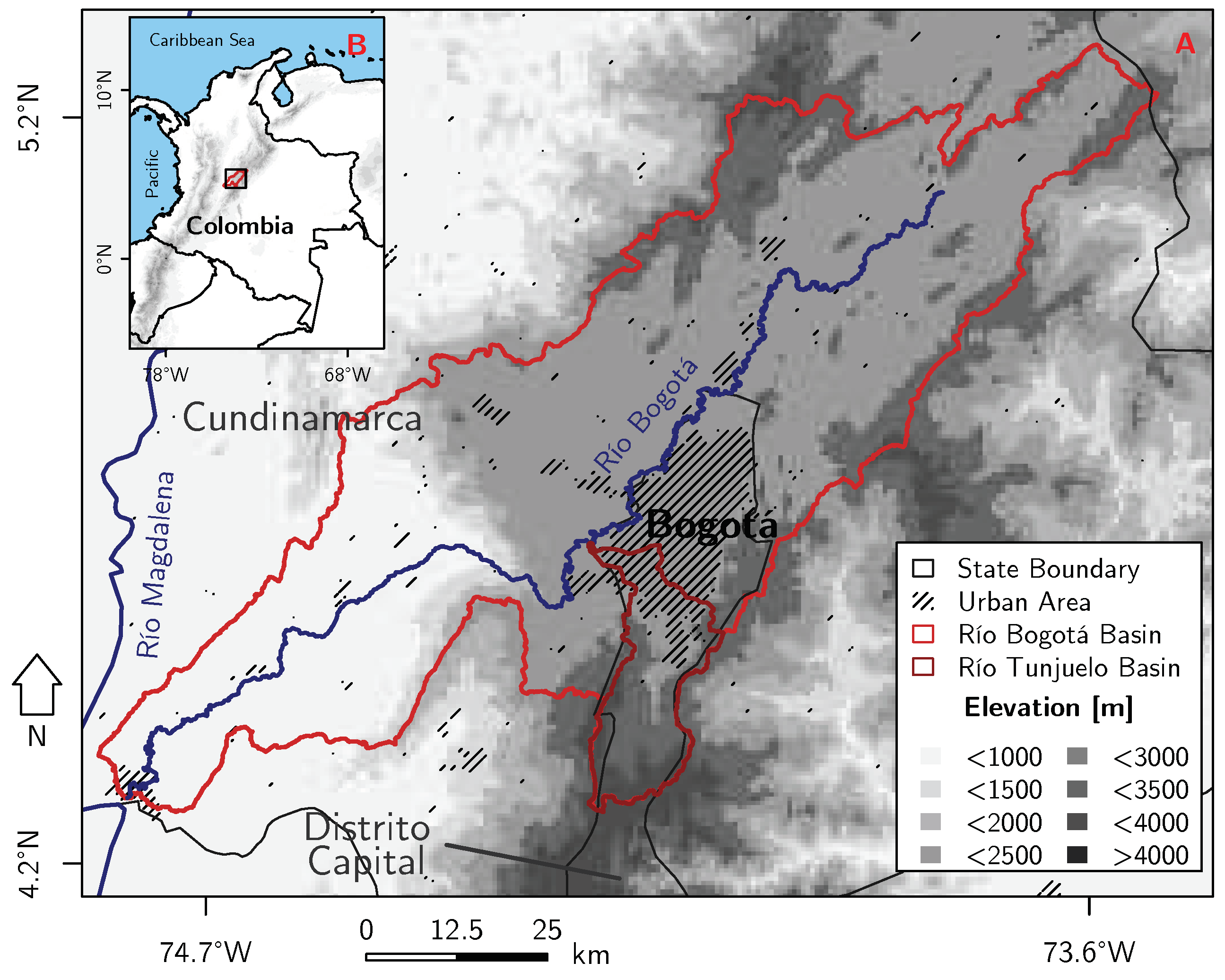
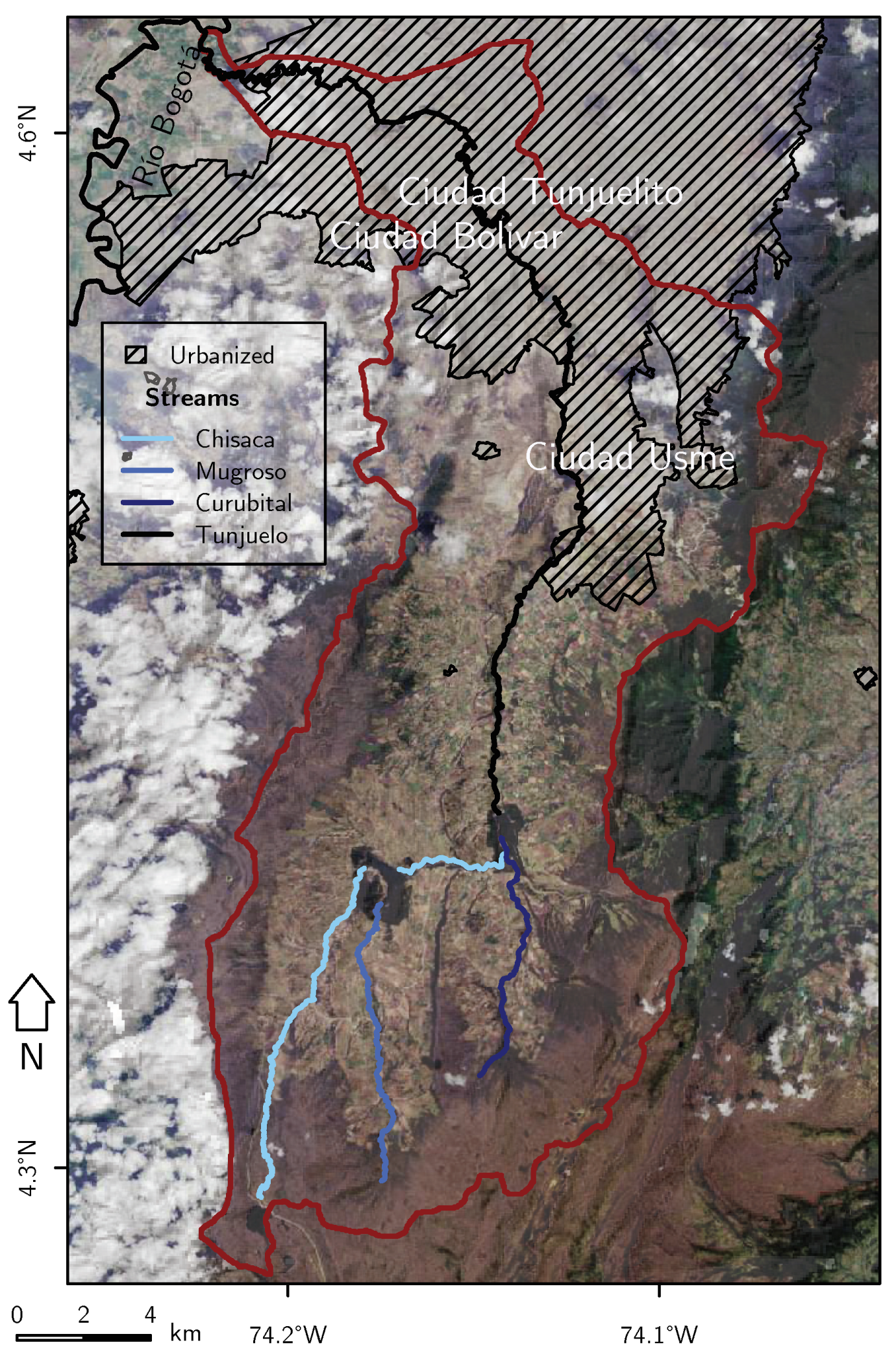
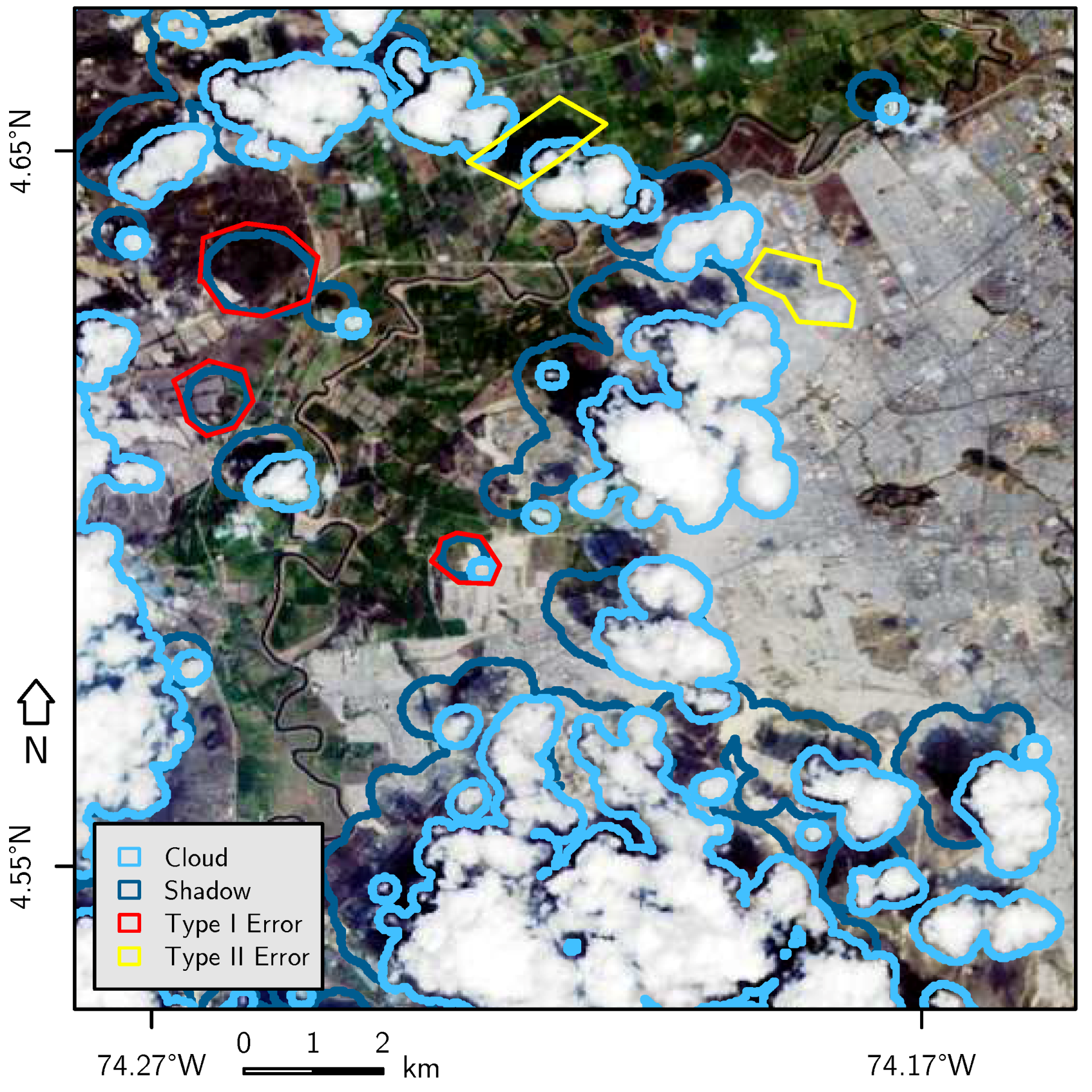
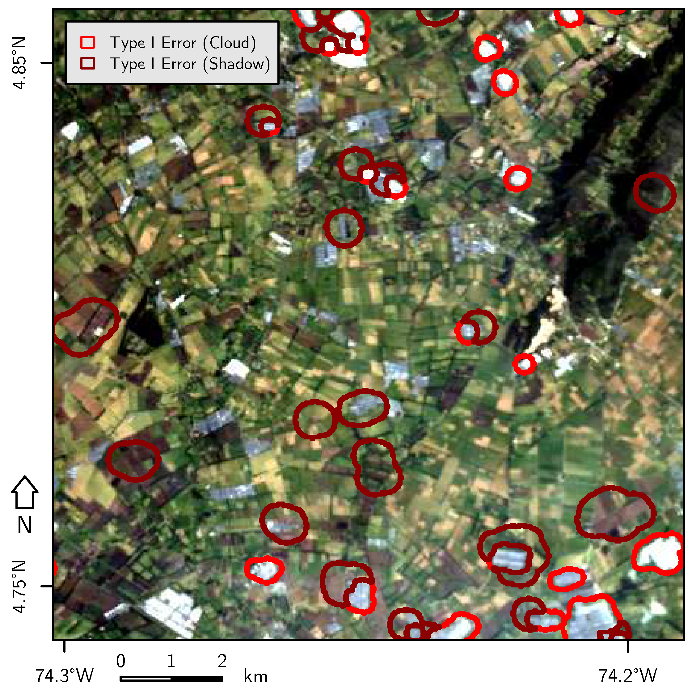
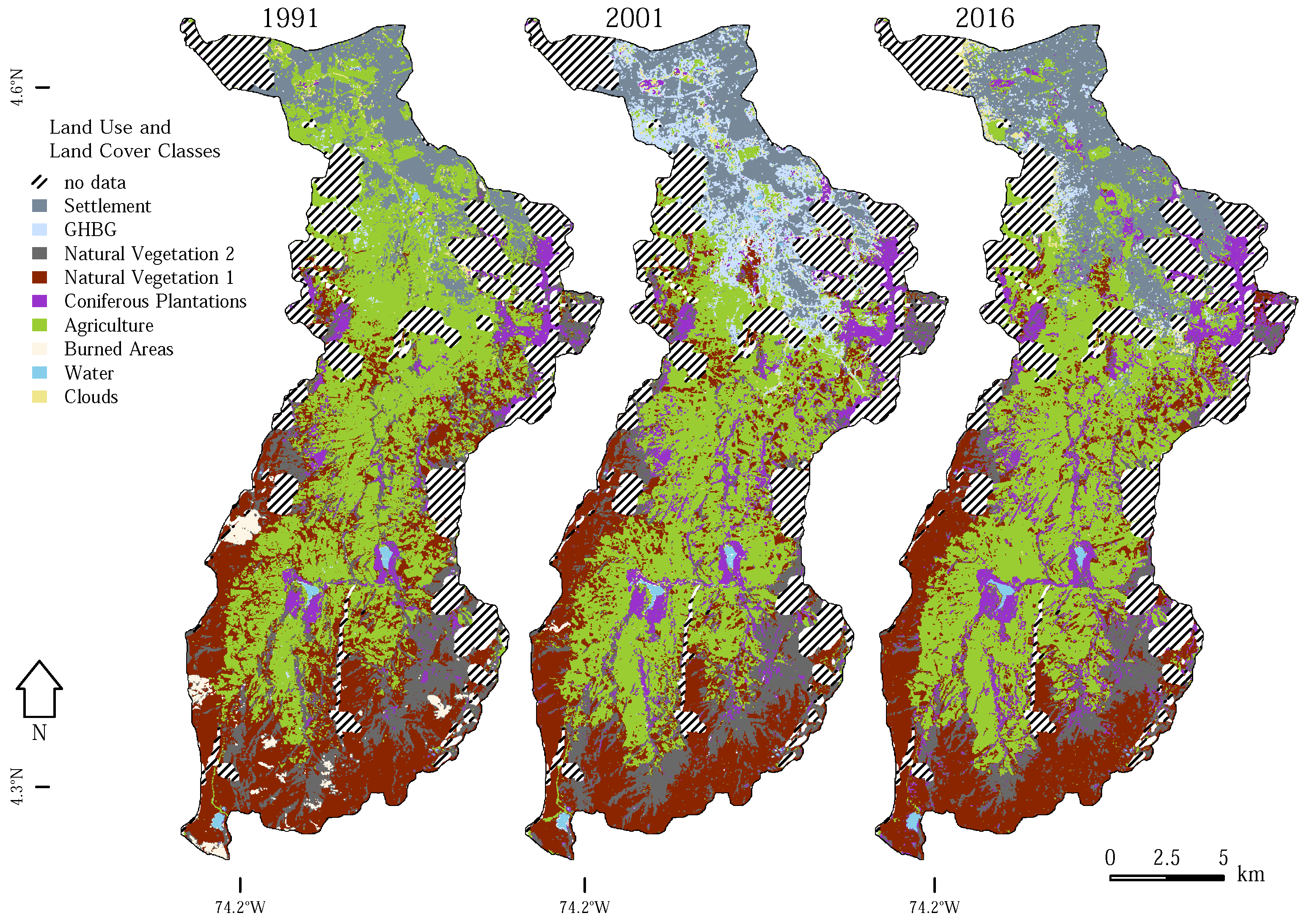
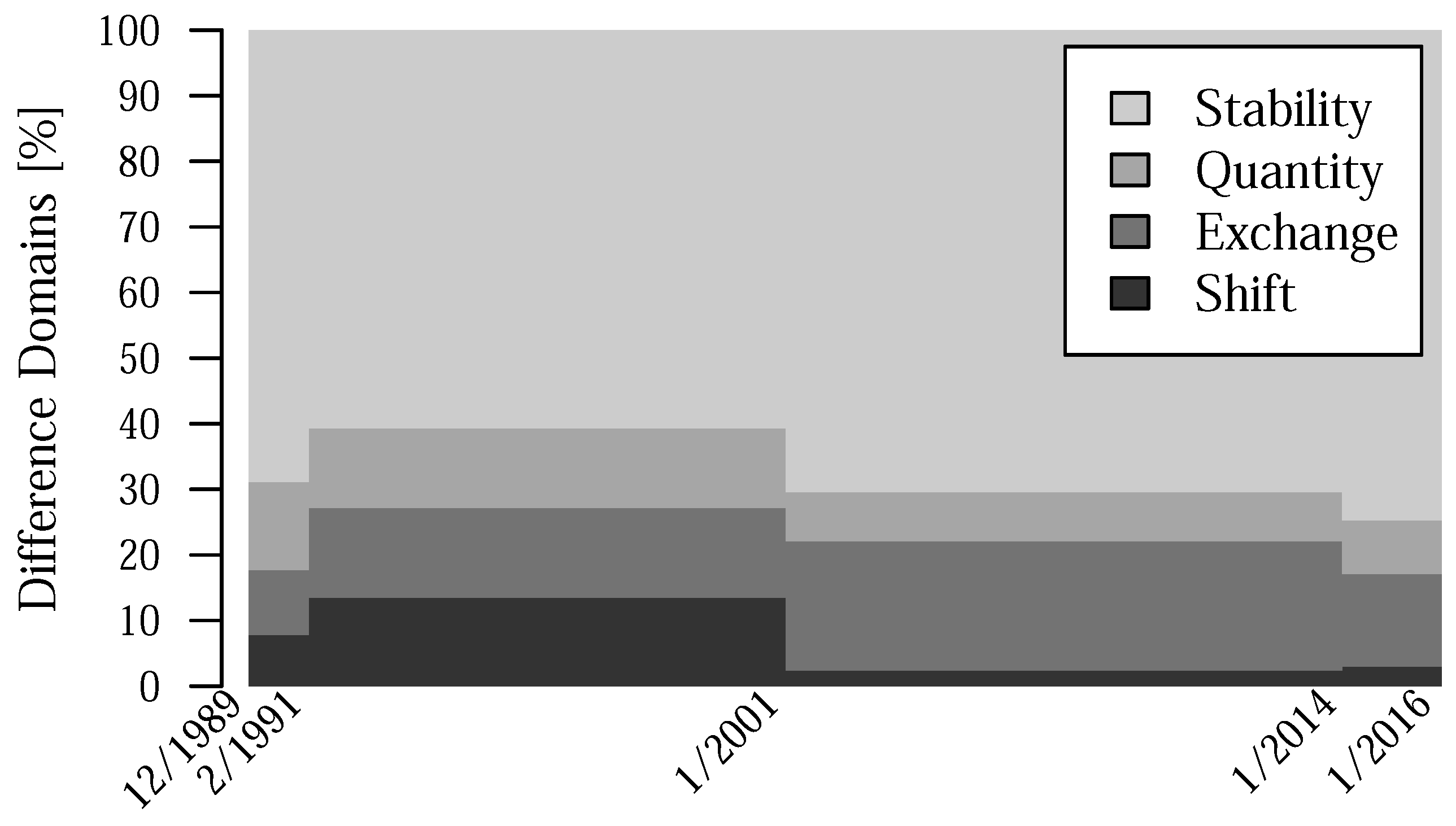
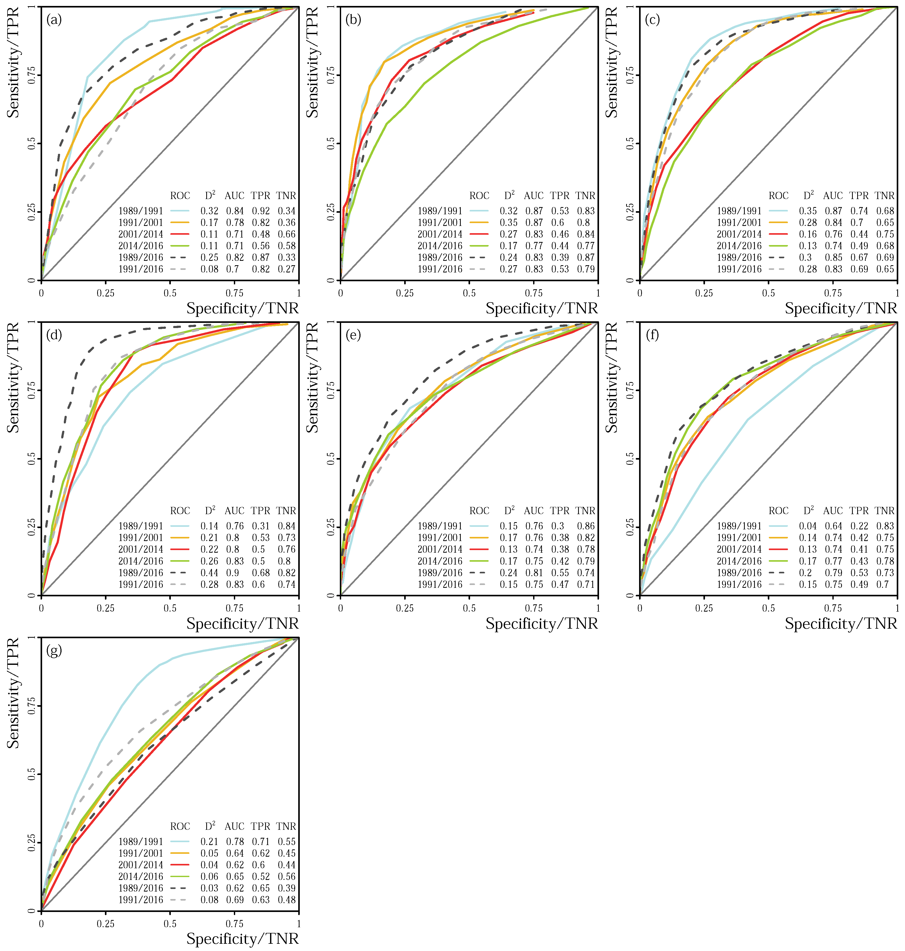
Table 1.
Available Landsat scenes.
| Date | Sensor | Cloud Cover [%] |
|---|---|---|
| 22 December 1989 | TM | 10.0 |
| 19 February 1991 | TM | 30.0 |
| 29 January 2001 | TM | 0.0 |
| 1 January 2014 | OLI | 20.51 |
| 23 January 2016 | OLI | 46.86 |
Table 2.
Class description, class separation approach and relative spatial share of each land cover class from 1989 to 2016.
Table 2.
Class description, class separation approach and relative spatial share of each land cover class from 1989 to 2016.
| Spatial Extent [%] | |||||||
|---|---|---|---|---|---|---|---|
| Class | Class Description | Separation Approach | 1989 | 1991 | 2001 | 2014 | 2016 |
| GHBG | greenhouses appear as large complexes, bare ground is the land surface with exposed bright sandstone | derived from image interpretation, large variation in the digital numbers but with similar characteristics of the spectral curve | 1.7 | 0.3 | 8.5 | 5.7 | 1.3 |
| Settlement | densely populated areas, build-up areas or otherwise sealed areas | knowledge based classified in combination with visual image interpretation | 11.5 | 10.0 | 11.2 | 11.9 | 14.5 |
| Natural Vegetation 1 | Espeletia (frailejon) covered high-altitude ecosystem (Páramo) as stated in Diazgranados et al. [103], often on slopes, no very thick solum and rather shallow vegetation cover | knowledge based classified in combination with visual image interpretation | 29.6 | 32.9 | 22.5 | 21.0 | 23.7 |
| Natural Vegetation 2 | high vegetation cover, often shrubby, thicker solum than Nat. Vegetation 1 class, gradual transition to Nat. Vegetation 1 class, most likely Bosque Altoandino and other forest-like ecosystems occur here | knowledge based classified in combination with visual image interpretation | 13.0 | 15.4 | 15.5 | 14.2 | 11.8 |
| CP | coniferous plantations | knowledge based classified in combination with visual image interpretation | 6.9 | 2.9 | 6.2 | 5.8 | 7.2 |
| Agriculture | mostly agricultural fields and mosaics used for ranching and farming | mostly based on the ratio of red and near-infrared bands, derived from agricultural fields only | 36.0 | 35.6 | 34.7 | 40.6 | 40.8 |
| Burned Areas | burning scars of wildfires, mostly surrounded by Natural Vegetation 1 class | derived from very low reflectances in the visible spectrum and near-infrared | 0.7 | 1.2 | 0.2 | – | 0.1 |
| Clouds | derived from clouds | very high reflective values in blue band | 0.1 | 0.3 | 0.7 | 0.1 | 0.5 |
| Water | natural and artificial water bodies | very low reflectance, especially in near-infrared/infrared bands | 0.3 | 0.3 | 0.4 | 0.6 | 0.3 |
Table 3.
Synopsis from the Multiple Regression Analysis tables. The second column indicates the used predictors in the Multiple Regression Analysis for the tested time intervals. If a statistical relation between change of the land cover and a tested parameter exists, it appears significant in the regression tables for the distinct time interval. This table summarizes the classes Greenhouses and Bare Ground (GB), Settlement (SM), the combined classes Greenhouses and Bare Ground and Settlement (GBSM), Coniferous Plantations (CP), Natural Vegetation 1 (NV1), Natural Vegetation 2 (NV2), the combined classes Natural Vegetation 1 and Natural Vegetation 2 (NV) and, Agriculture class (AC). Highly significant results (p < 0.001) appear in boldface.
| Time Intervals | ||||||||
|---|---|---|---|---|---|---|---|---|
| Predictor | 1989–1991 | 1991–2001 | 2001–2014 | 2014–2016 | 1989–2016 | 1991–2016 | ||
| Terrain | Parameters | Elevation | NV1, NV | NV1, NV | NV1, NV | NV1, NV | ||
| Slope | NV2 | NV2 | NV1, NV2 | NV1 | ||||
| Aspect | NV1 | NV1 | NV1, NV | NV1, NV | NV1, NV | |||
| Profile Curvature | ||||||||
| Tangential Curvature | GB, GBSM | GB, GBSM | ||||||
| Distances | Distance to GHBG | SM, NV2 | SM | SM, NV2 | SM | SM, NV2 | SM, NV2 | |
| Distance to Settlement | NV1, NV2 | NV2 | NV1, NV | NV | ||||
| Distance to CP | NV2 | GB | GB, NV1, NV2 | GB, GBSM, NV1 | GB, GBSM, NV1, NV2 | GB, NV1, NV2 | ||
| Distance to Natural Vegetation 1 | SM, GBSM | SM, GBSM | SM, GBSM | SM, GBSM, GBSM | ||||
| Distance to Natural Vegetation 2 | GB, SM | GB, NV1 | SM | GB, NV1 | GB | NV1 | ||
| Distance to Agriculture | SM, NV, AC | SM, GBSM, NV1, NV, AC | SM, GBSM, NV1, NV, AC | SM, NV | SM, NV | NV1, NV | ||
| Distance to Burned Areas | NV1, NV2 | GBSM | SM, NV2, NV | SM, NV1, NV | SM, GBSM, AC | AC | ||
| Distance to Water | SM | SM | AC | AC | AC | |||
| Distance to Street | NV2 | GB, NV1, NV2 | SM | GB, NV1 | GB, SM, NV2 | SM, NV1, NV2 | ||
| Distance to Stream | NV2 | GB, NV1, NV2 | GB, NV1 | NV1 | ||||
| Soil Chemical and | Physical Parameters | Soil Cation Exchange Capacity | GB | GB, GBSM, NV1, NV | NV1, NV2, NV, AC | GB, GBSM, NV2, AC | GBSM, NV1, NV | |
| Soil Organic Carbon Content | SM | GB, SM, GBSM | GB, GBSM, NV | GBSM, NV2 | NV2, NV | GB, SM, GBSM, NV2, NV | ||
| Soil pH | GBSM, AC | GBSM, NV | GB, GBSM | GB, GBSM, NV | GBSM, NV | GBSM, NV, AC | ||
| Bulk Density | SM, GBSM | SM, GBSM | SM, GBSM | |||||
| Depth to Bedrock | AC | AC | ||||||
| Gravel Content | SM, NV2 | GBSM | SM, GBSM | NV2 | SM | |||
| Sand Content | AC | AC | ||||||
| Silt Content | GBSM | GBSM | NV1 | NV2 | GBSM, NV1, NV2 | |||
| Clay Content | NV | NV | ||||||
Table 4.
Estimation of accuracy for random forest land cover classification.
| Year | 1989 | 1991 | 2001 | 2014 | 2016 |
|---|---|---|---|---|---|
| Kappa Index | 0.964 | 0.953 | 0.959 | 0.985 | 0.974 |
© 2018 by the authors. Licensee MDPI, Basel, Switzerland. This article is an open access article distributed under the terms and conditions of the Creative Commons Attribution (CC BY) license (http://creativecommons.org/licenses/by/4.0/).
Share and Cite
MDPI and ACS Style
Anselm, N.; Brokamp, G.; Schütt, B. Assessment of Land Cover Change in Peri-Urban High Andean Environments South of Bogotá, Colombia. Land 2018, 7, 75. https://0-doi-org.brum.beds.ac.uk/10.3390/land7020075
AMA Style
Anselm N, Brokamp G, Schütt B. Assessment of Land Cover Change in Peri-Urban High Andean Environments South of Bogotá, Colombia. Land. 2018; 7(2):75. https://0-doi-org.brum.beds.ac.uk/10.3390/land7020075
Chicago/Turabian StyleAnselm, Norbert, Grischa Brokamp, and Brigitta Schütt. 2018. "Assessment of Land Cover Change in Peri-Urban High Andean Environments South of Bogotá, Colombia" Land 7, no. 2: 75. https://0-doi-org.brum.beds.ac.uk/10.3390/land7020075
Note that from the first issue of 2016, this journal uses article numbers instead of page numbers. See further details here.