Criteria to Confirm Models that Simulate Deforestation and Carbon Disturbance

Abstract

The Verified Carbon Standard (VCS) recommends the Figure of Merit (FOM) as a possible metric to confirm models that simulate deforestation baselines for Reducing Emissions from Deforestation and forest Degradation (REDD). The FOM ranges from 0% to 100%, where larger FOMs indicate more-accurate simulations. VCS requires that simulation models achieve a FOM greater than or equal to the percentage deforestation during the calibration period. This article analyses FOM’s mathematical properties and illustrates FOM’s empirical behavior by comparing various models that simulate deforestation and the resulting carbon disturbance in Bolivia during 2010–2014. The Total Operating Characteristic frames FOM’s mathematical properties as a function of the quantity and allocation of simulated deforestation. A leaf graph shows how deforestation’s quantity can be more influential than its allocation when simulating carbon disturbance. Results expose how current versions of the VCS methodologies could conceivably permit models that are less accurate than a random allocation of deforestation, while simultaneously prohibit models that are accurate concerning carbon disturbance. Conclusions give specific recommendations to improve the next version of the VCS methodology concerning three concepts: the simulated deforestation quantity, the required minimum FOM, and the simulated carbon disturbance.

1. Introduction

Computerized simulation models quantify the effects of conservation projects designed for Reducing Emissions from Deforestation and forest Degradation (REDD). A model simulates the deforestation and resulting greenhouse gas emissions that would likely occur without a conservation project. A project’s offset is the model’s simulated emissions minus the project’s actual emissions. Larger simulated emissions produce larger offsets. Therefore, it is essential to use an appropriate simulation model. A variety of models and techniques are available [1], but it is not immediately obvious how to select a model or its parameters. The National Research Council [2] emphasizes that selection criteria should relate to the model’s purposes [3]. A model’s purposes for REDD are to simulate deforestation and the resulting emissions. The Verified Carbon Standard (VCS) methodologies for unplanned deforestation recommends that model selection and confirmation use a metric called the Figure of Merit (FOM) [4]. This article analyzes the VCS criteria by examining the FOM’s ability to evaluate simulation models with respect to the goals of REDD.

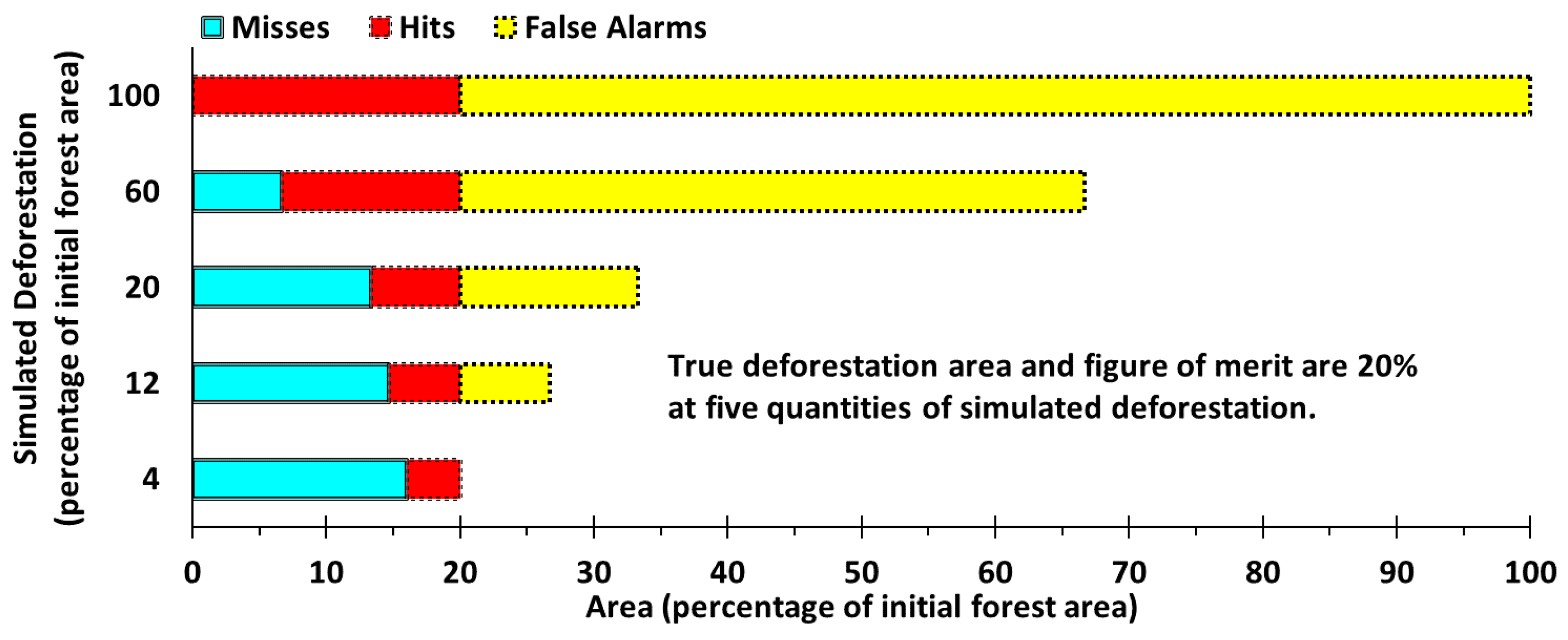
Figure 1 illustrates the FOM, also known as the Jaccard index. The spatial extent is the forest area at the start of the simulation, which Figure 1 shows as 100% on the horizontal axis. The quantity of true deforestation is 20%. Any particular simulation can select any quantity of simulated deforestation between 0% and 100%. The vertical axis shows five possible simulated quantities: 4%, 12%, 20%, 60%, and 100%. For each quantity, the simulation model allocates the simulated deforestation in space, typically in a raster map of pixels. Confirmation compares the map of true deforestation to the map of simulated deforestation. The VCS uses the word “confirmation” rather than “validation” to describe this particular procedure, because the VCS uses “validation” to refer to other types of procedures. A Miss is where a pixel has true deforestation but simulated forest persistence. A Hit is where a pixel has true deforestation and simulated deforestation. A False Alarm is where a pixel has true forest persistence but simulated deforestation. A Correct Rejection is where a pixel has true forest persistence and simulated forest persistence. The true deforestation is the union of Misses and Hits. The simulated deforestation is the union of Hits and False Alarms. Hits plus Correct Rejections is the percent correct at the end of the simulation, which is not a useful metric because percent correct fails to distinguish between correctly simulated change and correctly simulated persistence. Any metric that fails to distinguish Hits from Correct Rejections is potentially misleading, such as when the kappa index compares the two maps at the end of the simulation [5].

Equation (1) defines the FOM, which is a ratio. The numerator is the size of the intersection of True deforestation and Simulated deforestation, which is the size of the Hits. The denominator is the size of the union of True deforestation and Simulated deforestation, which is the size of the sum of Misses, Hits and False Alarms. The Total Error is the sum of Misses and False Alarms. This article reports FOM as a percentage. FOM ranges theoretically from 0% to 100%, where 0% means no intersection between True deforestation and Simulated deforestation while 100% means perfect intersection between True deforestation and Simulated deforestation. Figure 1 illustrates how various quantities of simulated deforestation can produce the same FOM value. FOM combines information concerning quantity and allocation into one metric, thus FOM fails to distinguish clearly between the concepts of quantity and allocation.

$$\begin{array}{ll}\mathrm{Figure}\mathrm{of}\mathrm{Merit}& =\left(\mathrm{True}\cap \mathrm{Simulated}\right)/\left(\mathrm{True}\cup \mathrm{Simulated}\right)\\ & =\mathrm{Hits}/\left(\mathrm{Misses}+\mathrm{Hits}+\mathrm{False}\mathrm{Alarms}\right)\\ & =\mathrm{Hits}/\left(\mathrm{Hits}+\mathrm{Total}\mathrm{Error}\right)\end{array}$$

(1)

The 2012 Verified Carbon Standard (VCS) VM0015 version 1.1 Methodology for Avoided Unplanned Deforestation [6] (p. 54) calls for “appropriate statistical techniques” to measure the fit of a simulation model. The VCS’s VM0015 reads, “Preference should be given to techniques that assess the accuracy of the prediction at the polygon level, such as the predicted quantity of total deforestation within the project area as compared to the observed one”, where the observed one is presumably the true quantity of deforestation during the confirmation period. The VM0015 goes on to specify, “One of the assessment techniques that can be used is the ‘Figure of Merit’”. VCS’s methodologies VM0015 and VMD0007 for unplanned deforestation [7] say that the FOM “must be used as the criterion for selecting the most accurate Deforestation Risk Map to be used for predicting future deforestation” and “The minimum threshold for the best fit as measured by the Figure of Merit (FOM) shall be defined by the net observed change in the reference region for the calibration period of the model. Net observed change shall be calculated as the total area of change being modeled in reference region during the calibration period as percentage of the total area of the reference region. The FOM value shall be at least equivalent to this value.” If the FOM value is below the minimum threshold, then VM0015 says “the project proponent must demonstrate that at least three models have been tested, and that the one with the best FOM is used”, while VMD0007 says “project proponents must provide evidence that the FOM achieved is consistent with comparable studies given the nature of the project area and the data available.” The calibration period defines the minimum threshold for the FOM value, while the calculated FOM applies to the confirmation period, which might have a duration and trends different from the calibration period. If the trends during the calibration period are different from the confirmation period, then VMD0015 allows a procedure where randomly selected tiles serve for both calibration and confirmation during a single period, in which case the resulting FOM indicates the model’s ability to simulate across space, not through time.

The VCS documents cite References [8] and [9], for which the first author is Pontius. Those two articles reported FOMs less than 15% for cases that had less than 10% net change during the confirmation period, not the calibration period. Approved REDD projects under VCS Scope 14 have used the FOM nine times with values ranging from 0.06% to 11.70% [10]. Pontius initially considered the VCS’s minimum required threshold to be low before he interpreted the results in the article that you are now reading. Pontius considered the threshold as low because even a random allocation would produce a positive FOM. Furthermore, the VCS links its FOM criterion to the calibration period, while the VCS cites articles that relate the FOM to the confirmation period, thus the VCS criterion might allow FOM values that are less than the FOM expected from a randomly allocated simulation. VCS methodologies have changed over time. The previous version 1.0 of VM0015 [11] (p. 64) set the minimum threshold for FOM at 50% or 80% depending on the type of landscape. Pontius has seen only one case where FOM was as larger than 50% [12]. Pontius is also concerned that FOM focuses exclusively on the deforestation risk map, while the risk map’s purpose is to simulate carbon disturbance. FOM does not necessarily indicate ability to simulate carbon disturbance, and there is not necessarily a linear relationship between deforestation and carbon disturbance [13].

This article analyzes the FOM’s appropriateness to confirm models for REDD with particular attention to three concepts: the simulated deforestation quantity, the required minimum FOM, and the simulated carbon disturbance. Section 2 describes the mathematical properties of the FOM with respect to the quantity and allocation of deforestation and the resulting carbon disturbance. Section 3 reports results in theory generally and in practice for Bolivia. Section 4 discusses the results with respect to the current VCS criteria. Section 5 concludes with recommended improvements for the next version of VCS methodology.

2. Materials and Methods

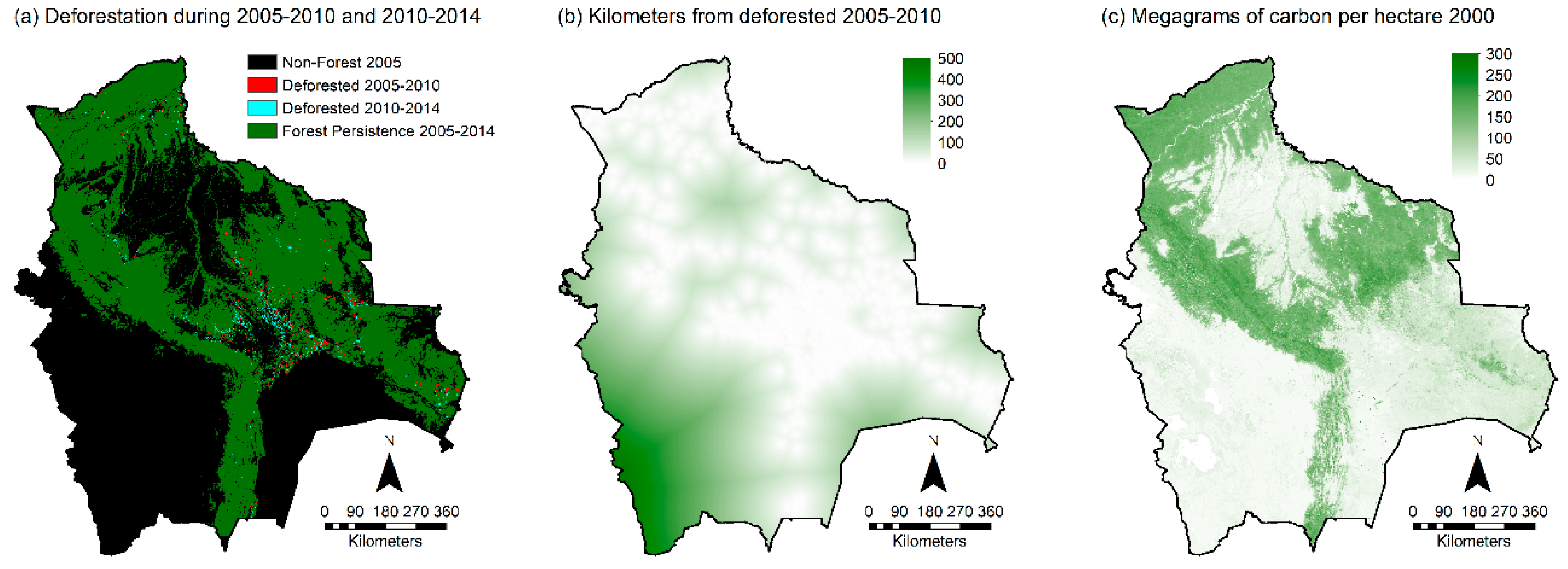
The case study of Bolivia has a data format that illustrates the generally applicable concepts. Figure 2 shows the materials, which are raster maps that have a spatial resolution of 990 m per pixel side. Figure 2a shows deforestation according to a combination of data sources concerning land cover [14] and forest change [15]. The reference region is the forest area at 2005. The calibration period is 2005–2010, and the confirmation period is 2010–2014. Deforestation during the calibration period was 1.1% of the forest area at 2005, equivalent to 1.1 thousand square kilometers per year. Deforestation during the confirmation period was 1.5% of the forest area at 2010, implying deforestation accelerated to 1.8 thousand square kilometers per year. Figure 2b shows distance from the deforestation that occurred during the calibration period. Figure 2c shows carbon stocks in terms of density of above ground biomass circa 2000 [16].

Simulation models typically use information from the calibration period to extrapolate deforestation during a confirmation period. Each possible simulation selects a quantity of simulated deforestation, and then allocates the selected quantity within the forest at the start of the confirmation period. For the Bolivia example, extrapolation of a constant annual area deforested during the calibration period would imply that deforestation during the confirmation period is 1% of the forest at the start of the confirmation period. This article examines the full range for the simulated deforestation quantity, from 0% to 100% in steps of 0.5% of the forest at 2010. For each simulated quantity, this article considers various possible allocations. Figure 2b dictates the Proximity allocation, which prioritizes deforestation closest to the deforestation during the calibration period. Figure 2c dictates the Lowest Carbon allocation, which prioritizes deforestation at the lowest carbon densities, similar to the conservative approach that the VCS’s VMD0007 recommends [7] (p. 27). Figure 2c dictates also the Highest Carbon allocation, which prioritizes deforestation at the highest carbon densities. The Lowest Carbon and Highest Carbon allocations create lower and upper bounds concerning simulated carbon disturbance. The purpose of the Lowest and Highest Carbon allocations is to create lower and upper bounds concerning how simulated deforestation can influence carbon disturbance. The bounds reveal how simulated allocation compares to simulated quantity in terms of their influences on carbon disturbance. The Lowest and Highest Carbon allocations do not necessarily portray the most likely allocations. The Random allocation is the mathematical expectation for a model that allocates pixels at random. Comparison of the simulated deforestation with the true deforestation during the confirmation period produces Misses, Hits, False Alarms and Correct Rejections [17]. Those four measurements are inputs to various confirmation metrics, including the FOM.

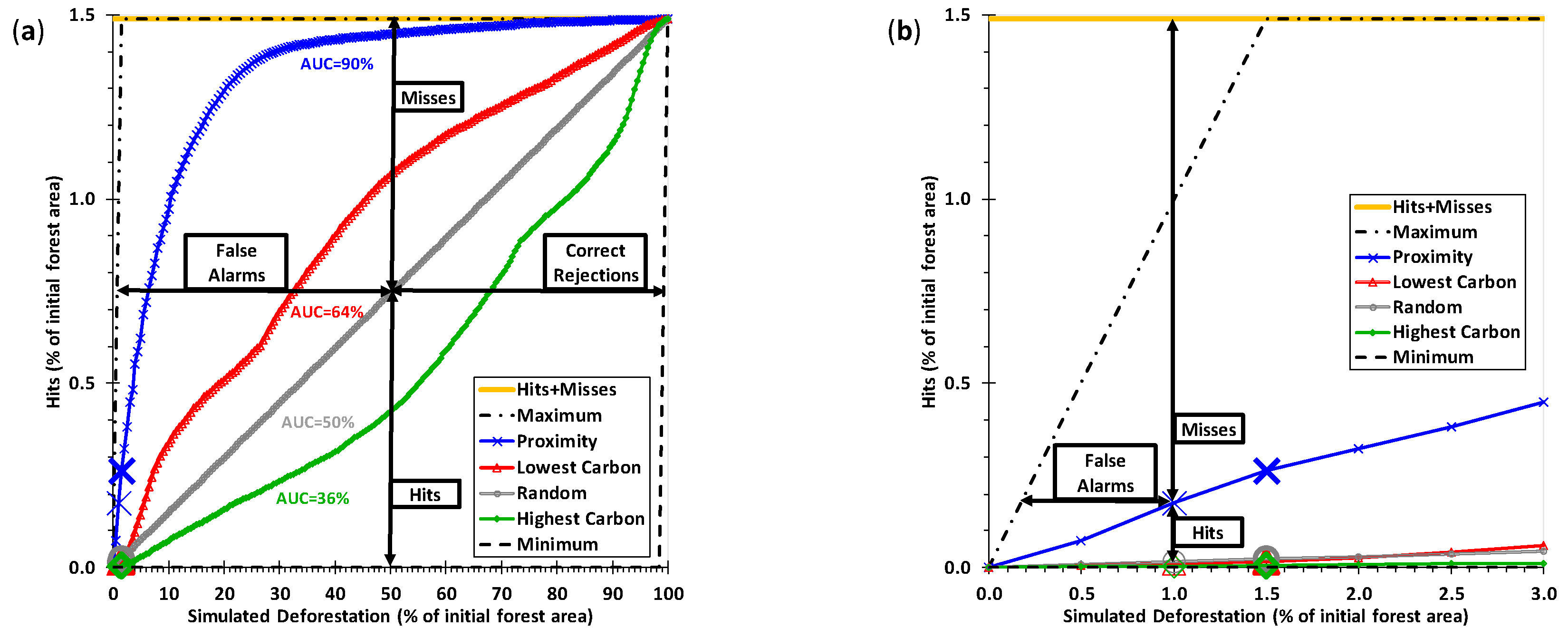
Figure 3, Figure 4, Figure 5, Figure 6 and Figure 7 show how this article’s methods proceed. The horizontal axis is the quantity of simulated deforestation during the confirmation period expressed as a percentage of the forest area at the start of the confirmation period. Figure 3, Figure 4, Figure 5, Figure 6 and Figure 7 come in pairs where the horizontal axis of (a) ranges from 0% to 100% and (b) ranges from 0% to 3%, which is double the true deforestation quantity. Part (a) of the figures shows the full range to explain the mathematical behavior of the metrics. Part (b) of the figures shows a zoomed in range to focus near the true and extrapolated quantity of deforestation during the confirmation period. Each of the four allocations has a bold marker, which indicates the true deforestation quantity during the confirmation period. Immediately to the left of each bold marker for each allocation is an enlarged marker, which indicates the deforestation quantity extrapolated from the calibration period. This article’s Supplementary Materials contain the raster maps and a spreadsheet that links the data to the figures below.

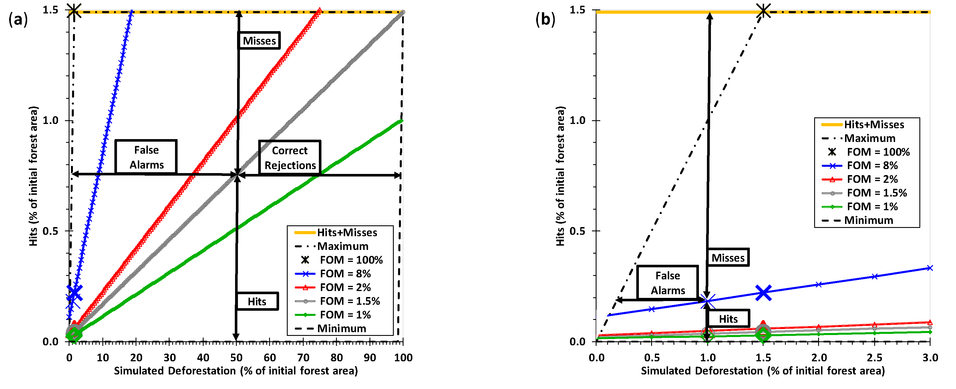
Figure 3 shows the Total Operating Characteristic (TOC) for the various allocations: Proximity, Lowest Carbon, Random and Highest Carbon. The TOC’s space distinguishes between the concepts of quantity and allocation [18]. The horizontal axis communicates the concept of quantity, while the vertical axis communicates the concept of allocation. The TOC plots Hits versus the quantity of simulated deforestation. Hits range on the vertical axis from zero to the true deforestation quantity, which is 1.5% for Bolivia. The true deforestation quantity dictates the Minimum and Maximum bounds, which form a parallelogram. The Maximum bound is where the simulated allocation is as accurate as possible. The Maximum bound begins at the origin and then increases Hits but not False Alarms as the simulated quantity increases until the simulated quantity matches the true deforestation quantity at the upper left corner of the Maximum bound. The Maximum bound increases False Alarms as the deforestation quantity increases to the right of its corner point. The Minimum bound is where allocation is as erroneous as possible. The Minimum bound begins at the origin and then increases False Alarms but not Hits as the simulated quantity increases to the lower right corner of the Minimum bound. The Minimum bound then increases Hits as the deforestation quantity increases to the right of its corner point. The arrows illustrate how each point in the TOC space corresponds to a combination of Hits, Misses, False Alarms and Correct Rejections. Hits is the vertical distance between the point and the horizontal axis. Misses is the vertical distance between the point and the top horizontal line that denotes Hits plus Misses. False Alarms is the horizontal distance between the point and the left Maximum bound. Correct Rejections is the horizontal distance between the point and the right Minimum bound. The quantity of simulated deforestation is Hits plus False Alarms. The top segment of the Maximum bound is Hits plus Misses. The left segment of the Maximum bound is the one-to-one line where Hits equals the simulated quantity, which is where False Alarms are zero. The Random allocation is always a straight line from the origin to the upper right corner of the TOC space. Each allocation produces a curve. The Area Under Curve (AUC) is a summary metric that is equal to the area under the TOC curve within the bounding parallelogram divided by the area of the bounding parallelogram. The Maximum bound has AUC of 100%. The Random allocation has AUC of 50%. The Minimum bound has AUC of 0%. The AUC of the TOC is identical to the AUC of the less-informative Relative Operating Characteristic (ROC) [19], which has become popular to assess the accuracy of allocation models [20]. Software exists in the language R for the TOC and in several additional packages for the ROC [21]. The arrows in Figure 3b show the point where the simulated quantity matches the extrapolated quantity. The behavior of each curve near this point reveals how the simulated quantity compares to the simulated allocation in terms of their influences on Misses, Hits, False Alarms and Correct Rejections.

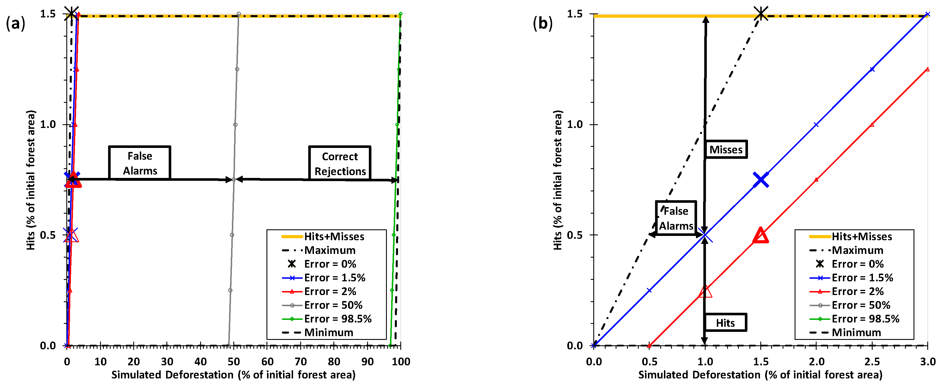
Figure 4 shows how TOC’s space relates to the total error, which is equal to Misses plus False Alarms and is equal to quantity error plus allocation error [5]. Quantity error is the absolute difference between the simulated quantity and the true quantity of deforestation [22]. Quantity error is zero when the simulated deforestation quantity equals the true deforestation quantity. Quantity error increases one unit for each absolute unit that the simulated deforestation quantity deviates from the true deforestation quantity. Allocation error measures the degree to which the allocation is suboptimal. Allocation error is positive when both Misses and False Alarms are positive; allocation error is zero when either Misses or False Alarms are zero. The Maximum bound shows where allocation is optimal, thus where allocation error is zero. Allocation error increases two units for each unit that Hits decrease from the Maximum bound, because allocation error forms from pairs of Misses and False Alarms [5]. The star at the upper left corner of the Maximum bound marks the point where the simulated deforestation quantity matches the true deforestation quantity and the allocation is optimal, which is the only point where total error is 0%. Total error is 100% at only the lower right corner point of the Minimum bound. Various selections of constant total error form parallel lines in the TOC space. For a constant size of error, Equation (2) reveals that Hits is a linear function of the simulated quantity, where: s = the simulated quantity of deforestation as a proportion of the initial forest; T = the true quantity of deforestation as proportion of the initial forest ≠ 0; and E = the total error as a proportion of the initial forest.

Hits = (s + T − E)/2

(2)

Figure 5 shows lines for constant FOMs within in the TOC space. A constant FOM forms a line from a point on the left bound to a point on either the right bound or the top bound. Larger FOMs form lines closer to the upper left corner, while smaller FOMs form lines closer to the horizontal axis. If FOM equals the true deforestation quantity, then the line extends from the origin to the upper right corner, which is identical to the Random allocation TOC line. Equation (3) shows how Hits is a linear function of the simulated quantity for a constant FOM, where F = the FOM as a proportion < 1.

Hits = (s + T)F/(1 − F)

(3)

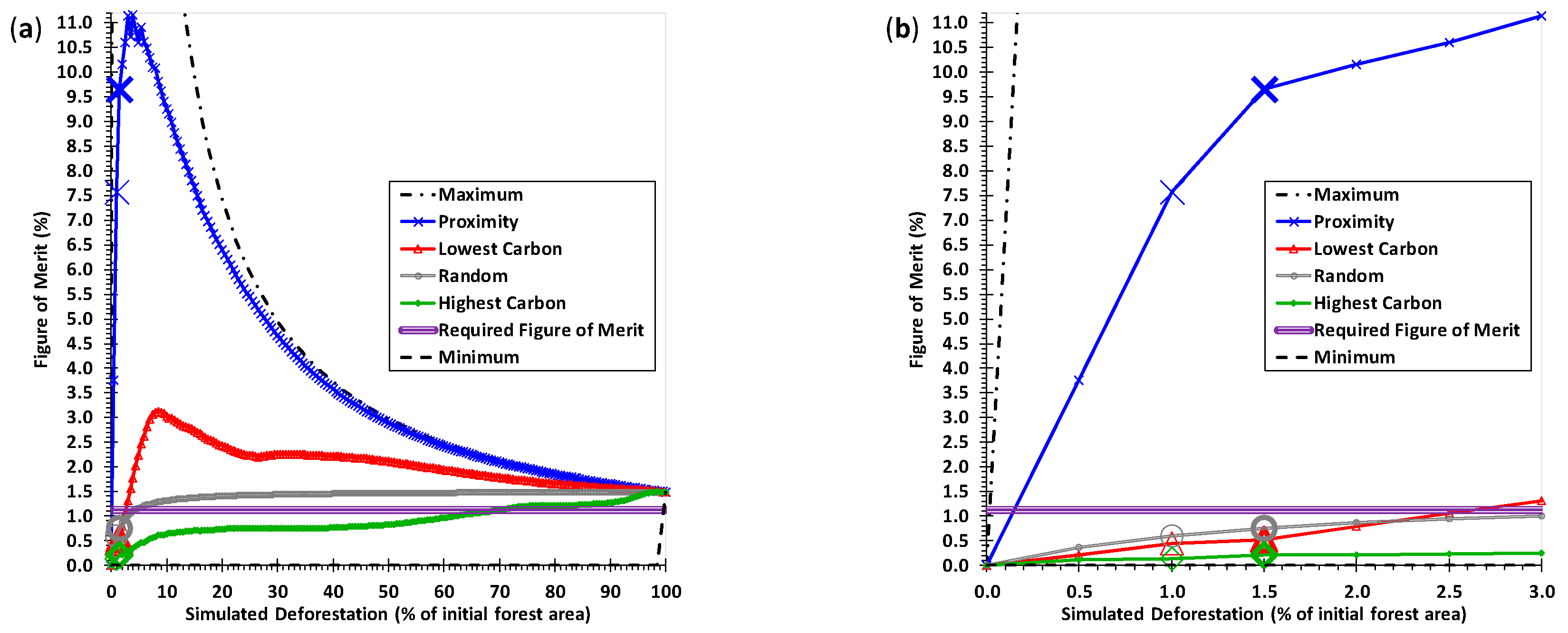
Figure 6 shows FOM versus the quantity of simulated deforestation. VCS methodology requires that a simulation model attain FOM greater than or equal to the percent deforestation during the calibration period, which is 1.1% for Bolivia. Therefore, Figure 6 shows a horizontal line at 1.1%. If simulated deforestation is greater than 70% of the initial forest area, then all allocations exceed the required FOM for Bolivia. Figure 6b shows that if the simulated quantity matches the true quantity of deforestation, then the Proximity allocation has FOM of 9.7% while the other three allocations have FOM values less than the required FOM. FOM for the Lowest Carbon allocation is below the required FOM until the simulated deforestation increases to double the true deforestation. Equations (4)–(6) define the mathematical behavior of the FOM as a function of s and T. Equation (4) describes how the Maximum FOM approaches one as the simulated deforestation approaches the true deforestation proportion during the confirmation period. Equation (5) shows that the FOM of the Random allocation is always less than or equal to T. Equations (4)–(6) describe how all allocations’ FOMs approach the true deforestation proportion T during the confirmation period as the proportion of simulated deforestation s approaches one.

$$\begin{array}{l}\mathrm{If}s\le T,\mathrm{then}\mathrm{Maximum}\mathrm{Figure}\mathrm{of}\mathrm{Merit}=s/T,\\ \mathrm{else}\mathrm{Maximum}\mathrm{Figure}\mathrm{of}\mathrm{Merit}=T/s\end{array}$$

(4)

Random Figure of Merit = sT/(s + T − sT) = sT/[s + T(1 − s)] ≤ T

(5)

Minimum Figure of Merit = MAXIMUM(0, s + T − 1)/s

(6)

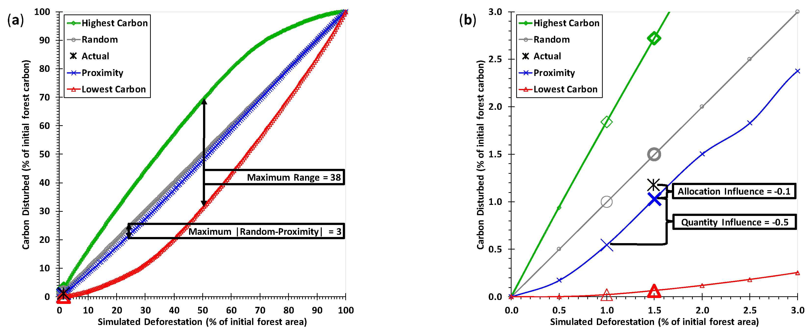
Figure 7 is a leaf graph that shows carbon disturbed versus the quantity of simulated deforestation [23]. The carbon disturbed is the mass of carbon at the locations where the model simulates deforestation. Both axes of the leaf graph range from 0% to 100%, because the carbon disturbed ranges from zero to all of the mass of the carbon in the initial forest, as the simulated deforestation ranges from 0% to 100% of the initial forest. The Random allocation forms a straight line from the origin to the upper right corner. The Lowest Carbon allocation and the Highest Carbon allocation form respectively lower and upper bounds in which the carbon disturbance must reside for any allocation. The shapes of the bounds inspire the name of the leaf graph. When simulated quantity is 50%, the Highest and Lowest Carbon allocation form their maximum range, which is 38 percentage points for Bolivia. When simulated quantity is 25%, the Random and Proximity allocations form their maximum range, which is 3 percentage points for Bolivia. The star in Figure 7b shows that the true deforestation was 1.5% of the initial forest area while the actual carbon disturbance was 1.2% of the initial carbon mass. This means that the actual deforestation during the confirmation period occurred in forests that had less than the average carbon density, which is a characteristic that the Proximity allocation portrays. When the simulated deforestation quantity matches true deforestation quantity, the less-than-perfect Proximity allocation explains all of the −0.1 deviation between simulated and actual carbon disturbance. When the simulated deforestation quantity matches extrapolated deforestation quantity, the quantity of deforestation is five times more influential than the Proximity allocation when forming the −0.6 deviation between simulated and actual carbon disturbance. These influences derive from Equations (7) and (8), where c(s) = simulated carbon disturbance at the simulated deforestation quantity s, c(T) = simulated carbon disturbance at the true deforestation quantity T; and A = actual carbon disturbance. Equation (7) attributes the deviation to two influences: Allocation and Quantity. Equation (8) shows how the deviation c(s) − A between simulated and actual carbon disturbance is the sum of its two influences.

$$\begin{array}{c}\mathrm{If}A\le c\left(T\right)\le c\left(s\right)\mathrm{or}c\left(s\right)\le c\left(T\right)\le A,\mathrm{then}\mathrm{Allocation}=c\left(T\right)-A\mathrm{and}\mathrm{Quantity}=c\left(s\right)-c\left(T\right),\\ \mathrm{Else}\mathrm{if}c\left(T\right)\le A\le c\left(s\right)\mathrm{or}c\left(s\right)\le A\le c\left(T\right),\mathrm{then}\mathrm{Allocation}=c\left(s\right)-A\mathrm{and}\mathrm{Quantity}=0,\\ \mathrm{Else}\mathrm{then}\mathrm{Allocation}=0\mathrm{and}\mathrm{Quantity}=c\left(s\right)-A.\end{array}$$

(7)

c(s) − A = Allocation + Quantity

(8)

The final step in this article’s methods compares Figure 6 and Figure 7. The next section reveals the results concerning the relationship between deforestation accuracy and carbon disturbed.

3. Results

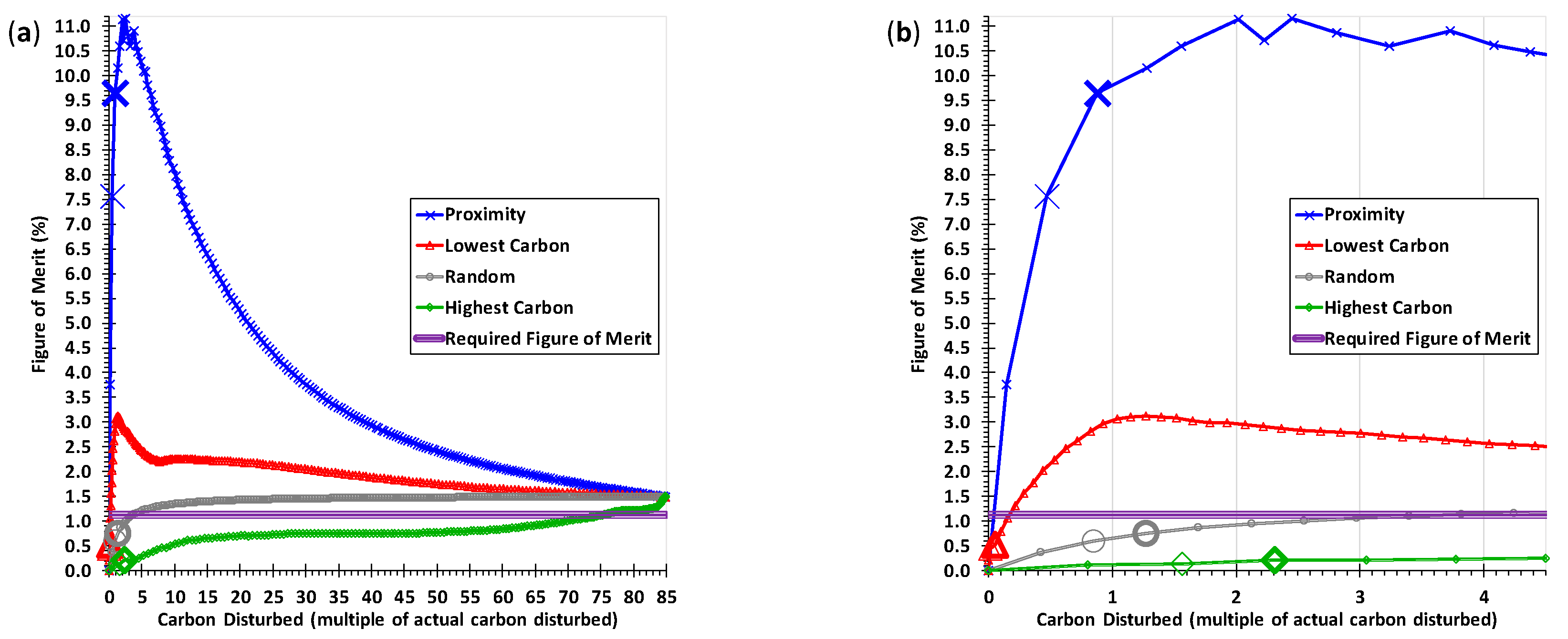
Figure 8 shows FOM versus simulated carbon disturbed. The horizontal expresses simulated carbon disturbance as a multiple of actual carbon disturbance, which is the mass of simulated carbon disturbance divided by the mass of actual carbon disturbance during the confirmation period. Therefore, one on the horizontal axis in Figure 8 is where simulated equals actual carbon disturbance. The maximum multiple on the horizontal is 85, because the initial forest has 85 times more carbon mass than the carbon mass disturbed during the confirmation period. The results show how FOM does not indicate accuracy of carbon disturbance. FOMs for the Random and Highest allocations increase monotonically with increasing carbon disturbance. All four allocations produce FOMs greater than the VCS’s required FOM when the simulated carbon disturbance is greater than 76 times the actual carbon disturbance. The Lowest Carbon allocation produces greater than the required FOM where the simulated carbon disturbance ranges from 0.22 to 85 times the actual carbon disturbance. The Proximity allocation produces greater than the required FOM where the simulated carbon disturbance ranges from 0.15 to 85 times the actual carbon disturbance. None of the allocations has its peak FOM at one on the horizontal axis, where simulated carbon disturbance is correct. The greatest FOM is 11.2% for the Proximity allocation where simulated carbon disturbance is 2.4 times the actual carbon disturbance. The bold markers indicate that Proximity simulates carbon disturbance more accurately than the other three allocations at the true quantity of deforestation. The enlarged markers to the immediate left of the bold markers indicate that the Random allocation simulates carbon disturbance most accurately at the extrapolated quantity of simulated deforestation, despite that the Random FOM is below the required FOM at that extrapolated quantity of deforestation.

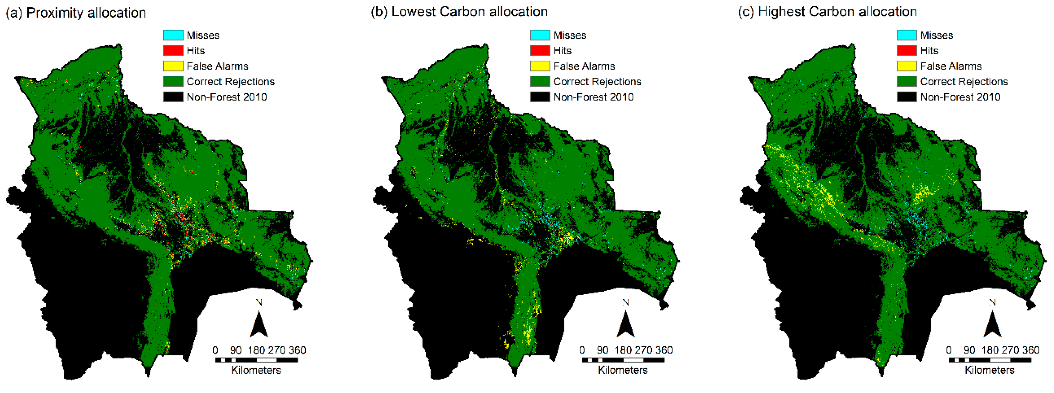
Figure 9 shows maps of confirmation results for three allocations where the simulated quantity is 3%, which is double the true percentage of deforestation during 2010–2014. The False Alarms are nearer the Misses for the Proximity allocation, compared to the other allocations. FOM is 11.1% in Figure 9a, 1.3% in Figure 9b, and 0.3% in Figure 9c. The FOMs in Figure 9a,b are above the required threshold of 1.1%, while the FOM in Figure 9c is not. The ratio of simulated carbon disturbance to actual carbon disturbance is 2.0 in Figure 9a, 0.2 in Figure 9b, and 4.5 in Figure 9c.

4. Discussion

VCS methodology VM0015 version 1.0 required FOM to be at least 50%, which would have prohibited all four allocations for the Bolivia case. VCS’s VM0015 version 1.1 and VMD0007 have a different requirement for FOM, which implies the FOM for Bolivia must be at least 1.1%. This threshold would permit the Proximity allocation but would still prohibit the Low Carbon, Random and High Carbon allocations. The Proximity allocation simulates deforestation on the 2010 forest that had less that average carbon density, which is what actually occurred. In fact, the Proximity allocation simulates 0.88 times the actual mass of carbon disturbance when the quantity of simulated deforestation matches the true quantity of deforestation. Thus, the most recent version of the VCS methodology allows an under prediction of the actual carbon disturbance in Bolivia by 12%, which researchers might consider acceptable. Nevertheless, analysis of FOM’s mathematical behavior reveals that VM0015 version 1.1 and VMD0007 have room for improvement concerning three concepts. These three concepts apply to modeling in ways that extend beyond REDD projects.

The first concept concerns the simulated deforestation quantity during model confirmation. A single deforestation risk map can have various FOMs depending on the simulated deforestation quantity. The risk map’s purpose is to specify allocation, not quantity. Therefore, if one were to focus on a single quantity, then it makes sense to select a quantity that allows for the most informative assessment of allocation. The current VCS methodology selects the deforestation risk map that has the largest FOM at the extrapolated deforestation quantity. However, the extrapolated deforestation quantity can vary depending on the calibration period and the method of extrapolation [24]. The true deforestation quantity is the only point that allows the maximum possible range for FOM to assess the ability of a risk map to allocate deforestation during the confirmation period. If a reader misconstrues the VCS methodology to mean that the modeler must select the quantity of simulated deforestation that maximizes FOM, then the selected quantity can deviate substantially from the true deforestation quantity. For example, the maximum overall FOM for Bolivia occurs when the simulated quantity is 2.7 times the true quantity of deforestation. Other quantities of simulated deforestation can give additional insights. Therefore, TOC curves are helpful to show how the simulated quantity influences the size of Hits. The TOC space shows that the maximum possible range for Hits exists where the simulated deforestation proportion s is between the true deforestation proportion T and 1 − T. However, the extrapolated quantity might not be in that range, as is the case for Bolivia. The allocation that has the largest size of Hits at a particular quantity is the allocation that has largest FOM at that quantity. Other accuracy metrics besides FOM also reach their largest values at a given quantity when Hits are largest. For example, percentage correct between the simulated deforestation and the true deforestation is largest when Hits is largest at any fixed simulated quantity. The AUC of the TOC and the shape of the TOC curves can be helpful to distinguish among various allocations [25], especially when the best allocation at the true deforestation quantity differs from the best allocation at other deforestation quantities. The take home message is that modelers should interpret the TOC, because the TOC offers helpful insights by examining various deforestation quantities.

The second concept concerns the required minimum FOM. The VCS requires that FOM be at least the percentage of the net observed change in the reference region for the calibration period. If “net observed change” means forest gain minus forest loss, then net observed change could be negative or zero, in which case any allocation would qualify, because FOM is always greater or equal to zero. The meaning of “net observed change” is ambiguous in the VCS documents concerning the meaning of “net”. Pages 7–8 of VCS’s VM0015 show reference regions that contain a category called “No-Forest”, where presumably forest could gain. Page 17 of VM0015 defines the reference region as “the spatial delimitation of the analytic domain from which information about rates, agents, drivers, and patterns of land-use and land-cover change (LU/LC-change) will be obtained, projected into the future and monitored”. Therefore, LU/LC-change might conceivably include forest gain. However, page 7 of VM0015 defines the reference region as “the analytical domain from which information on historical deforestation is extracted and projected into the future to spatially locate the area that will be deforested in the baseline case.” Therefore, it seems that that “net observed change” in VM0015 means forest loss, despite the fact that “net observed change” includes losses and gains among all categories in the journal article that VM0015 cites [9]. The VCS language should have a single clear definition of reference region. Also, if the VCS uses the word “net”, then the VCS should have a clear definition of “net”. Moreover, the VCS compares the FOM during the confirmation period to the deforestation percentage during the calibration period. If the deforestation percentage during the calibration period is less than the deforestation percentage during the confirmation period, then Equation (5) shows how the VCS could permit allocations that are less accurate than a random allocation, as the Bolivia example illustrates. Most importantly, modelers must define a clear criterion for model performance that matches the purpose of the model.

The third concept concerns how the quantity and allocation of deforestation influences carbon disturbance. The VCS methodology for model selection focuses on deforestation, but a REDD project aims to reduce carbon disturbance. The FOM indicates the accuracy of deforestation, not of carbon disturbance. If the FOM is 100%, then the simulated carbon disturbance is accurate; however, the converse is not true. An accurate prediction of carbon disturbance can exist when FOM is 0%. Furthermore, FOM combines quantity error and allocation error into one metric, but quantity and allocation can have different influences on carbon disturbance. For example, Bolivia’s leaf graph illustrates how the extrapolated quantity has five times more influence than the Proximity allocation on the deviation between simulated and actual carbon disturbance. If carbon density is homogenous, then deforestation quantity dictates carbon disturbance while deforestation allocation does not influence the carbon disturbance. Thus, a particular allocation might simulate carbon disturbance accurately even when the allocation fails to qualify according to current VCS methodologies. For example, a Random allocation is more accurate than the Proximity allocation for simulating carbon disturbance at the extrapolated quantity for Bolivia; however, the Random allocation fails to achieve the required FOM at the extrapolated quantity while the Proximity achieves the required FOM. Furthermore, randomized allocations have variation, thus some randomized allocations might be as accurate as the Proximity allocation in terms of carbon disturbance. A high requirement for FOM can defeat the goal to simulate carbon disturbance accurately. Even if carbon density is homogenous, then simulated allocation can still be important to show how much of the simulated deforestation falls into the REDD project area as opposed to outside the project area; however, allocation error within the project area would not influence the mass of carbon disturbance within the project area. The main point is that modelers must measure the influence of quantity specification relative to the influence of allocation specification, because quantity error and allocation error might not be equally important for the purpose of the model.

Future research should address uncertainties in at least two respects. First is to incorporate uncertainty concerning the carbon stocks. Sensitivity analysis could quantify how uncertainty in the carbon stocks compares to uncertainty in the simulated deforestation when simulating carbon disturbance. Second is to translate the simulated carbon disturbance into greenhouse gas emissions, because the ultimate goal of REDD projects is to reduce emissions.

5. Conclusions

This article examines the Figure of Merit and related criteria to confirm deforestation simulation models for REDD. The FOM can be appropriate when interpreted properly to compare various simulations of deforestation, but the FOM does not necessarily indicate the accuracy of carbon disturbance. The next version of VCS methodology should have improvements concerning three concepts.

The first concept concerns the simulated deforestation quantity. VCS’s VM0015 version 1.1 specifies, “Preference should be given to techniques that assess the accuracy of the prediction at the polygon level, such as the predicted quantity of total deforestation within the project area as compared to the observed one.” The next version of that rule should be “Preference should be given to techniques that assess the accuracy of the prediction at the true quantity of deforestation within the project area.” It is not clear how to assess accuracy at the polygon level [26], especially when the elements of a raster map are pixels. If modelers consider a single quantity, then the true quantity of deforestation is the quantity that distinguishes best among allocation models. A related VCS rule specifies, “The highest percent FOM must be used as the criterion for selecting the most accurate Deforestation Risk Map to be used for predicting future deforestation.” The phrase “The highest percent FOM must be used” should be “The highest FOM at the true quantity of deforestation is preferred to be used” for clarity, because a single risk map can have various FOM values depending on the simulated quantity. Other metrics offer other types of insights. A complimentary metric is the AUC of the TOC, which integrates results across various simulated quantities. The VCS methodology should recommend display and interpretation of TOC curves, to show how the simulated deforestation quantity affects model accuracy.

The second concept concerns the required minimum FOM. The current VCS rule specifies, “The minimum threshold for the best fit as measured by the Figure of Merit (FOM) shall be defined by the net observed change in the reference region for the calibration period of the model. Net observed change shall be calculated as the total area of change being modeled in reference region during the calibration period as percentage of the total area of the reference region. The FOM value shall be at least equivalent to this value.” Those three sentences should be, “The FOM’s minimum percentage must be larger than the deforestation area in the reference region during the confirmation period expressed as a percentage of the forest area in the reference region at the start of the confirmation period.” This modification would assure that the period of the required FOM matches the period of the confirmation data, which would assure that the simulated allocation is more accurate than a random allocation. The modification also would avoid possible confusion concerning the definition of net observed change.

The third concept concerns carbon disturbance. Future VCS methodology should use a leaf graph to show how the deforestation’s quantity and allocation influences the simulated carbon disturbance. The leaf graph shows the carbon disturbance across various quantities of deforestation, while simultaneously compares any proposed allocation to a random allocation within the range of possible allocations of deforestation. This is important because if the carbon density is homogenous across the initial forest area, then a random allocation of deforestation will produce the same mass of carbon disturbance as any other allocation of deforestation. This final recommendation would help to align the VCS criteria with the goals of REDD.

References

- Paegelow, M.; Camacho Olmedo, M.T.; Mas, J.-F.; Houet, T.; Pontius, R.G., Jr. Land change modelling: Moving beyond projections. Int. J. Geogr. Inf. Sci. 2013, 27, 1691–1695. [Google Scholar] [CrossRef] [Green Version]
- National Research Council. Advancing Land Change Modeling: Opportunities and Research Requirements; The National Academies Press: Washington, DC, USA, 2014. [Google Scholar]
- Brown, D.G.; Verburg, P.H.; Pontius, R.G., Jr.; Lange, M.D. Opportunities to improve impact, integration, and evaluation of land change models. Curr. Opin. Environ. Sustain. 2013, 5, 452–457. [Google Scholar] [CrossRef]
- Pontius, R.G., Jr.; Peethambaram, S.; Castella, J.-C. Comparison of Three Maps at Multiple Resolutions: A Case Study of Land Change Simulation in Cho Don District, Vietnam. Ann. Assoc. Am. Geogr. 2011, 101, 45–62. [Google Scholar] [CrossRef]
- Pontius, R.G., Jr.; Millones, M. Death to Kappa: Birth of quantity disagreement and allocation disagreement for accuracy assessment. Int. J. Remote Sens. 2011, 32, 4407–4429. [Google Scholar] [CrossRef]
- Pedroni, L. Approved VCS Methodology VM0015, v.1.1 Methodology for Avoided Unplanned Deforestation; Carbon Decisions International: Washington, DC, USA, 2012; p. 207. [Google Scholar]
- Winrock International. TerraCarbon VCS Module VMD0007 REDD, v.3.2 Methodological Module: Estimation of Baseline Carbon Stock Changes and Greenhouse Gas Emissions from Unplanned Deforestation (BL-UP); Winrock International: Little Rock, AR, USA, 2013. [Google Scholar]
- Pontius, R.G., Jr.; Walker, R.; Yao-Kumah, R.; Arima, E.; Aldrich, S.; Caldas, M.; Vergara, D. Accuracy assessment for a simulation model of Amazonian deforestation. Ann. Assoc. Am. Geogr. 2007, 97, 677–695. [Google Scholar] [CrossRef]
- Pontius, R.G., Jr.; Boersma, W.; Castella, J.-C.; Clarke, K.; de Nijs, T.; Dietzel, C.; Duan, Z.; Fotsing, E.; Goldstein, N.; Kok, K.; et al. Comparing the input, output, and validation maps for several models of land change. Ann. Reg. Sci. 2008, 42, 11–37. [Google Scholar] [CrossRef]
- West, T.A.P. On the Improvement of Tropical Forest-Based Climate Change Mitigation Interventions. Ph.D. Thesis, University of Florida, Gainesville, FL, USA, 2016. [Google Scholar]
- Pedroni, L. Approved VCS Methodology VM0015, v.1.0 Methodology for Avoided Unplanned Deforestation; Carbon Decisions International: Washington, DC, USA; p. 184. Available online: http://verra.org/wp-content/uploads/2018/03/VM0015-Avoided-Uplanned-Deforestation-v1.0.pdf (accessed on 10 September 2018).
- Pontius, R.G.; Castella, J.-C.; de Nijs, T.; Duan, Z.; Fotsing, E.; Goldstein, N.; Kok, K.; Koomen, E.; Lippitt, C.D.; McConnell, W.; et al. Lessons and Challenges in Land Change Modeling Derived from Synthesis of Cross-Case Comparisons. In Trends in Spatial Analysis and Modelling; Behnisch, M., Meinel, G., Eds.; Geotechnologies and the Environment; Springer International Publishing: Cham, Switzerland, 2018; Volume 19, pp. 143–164. ISBN 978-3-319-52520-4. [Google Scholar]
- Villamor, G.B.; Pontius, R.G., Jr.; van Noordwijk, M. Agroforest’s growing role in reducing carbon losses from Jambi (Sumatra), Indonesia. Reg. Environ. Chang. 2014, 14, 825–834. [Google Scholar] [CrossRef]
- Killeen, T.J.; Calderon, V.; Soria, L.; Quezada, B.; Steininger, M.K.; Harper, G.; Solórzano, L.A.; Tucker, C.J. Thirty Years of Land-cover Change in Bolivia. AMBIO J. Hum. Environ. 2007, 36, 600–606. [Google Scholar] [CrossRef] [Green Version]
- Hansen, M.C.; Potapov, P.V.; Moore, R.; Hancher, M.; Turubanova, S.A.; Tyukavina, A.; Thau, D.; Stehman, S.V.; Goetz, S.J.; Loveland, T.R.; et al. High-Resolution Global Maps of 21st-Century Forest Cover Change. Science 2013, 342, 850–853. [Google Scholar] [CrossRef] [PubMed]
- Saatchi, S.S.; Harris, N.L.; Brown, S.; Lefsky, M.; Mitchard, E.T.A.; Salas, W.; Zutta, B.R.; Buermann, W.; Lewis, S.L.; Hagen, S.; et al. Benchmark map of forest carbon stocks in tropical regions across three continents. Proc. Natl. Acad. Sci. USA 2011, 108, 9899–9904. [Google Scholar] [CrossRef] [PubMed] [Green Version]
- Camacho Olmedo, M.T.; Pontius, R.G., Jr.; Paegelow, M.; Mas, J.-F. Comparison of simulation models in terms of quantity and allocation of land change. Environ. Model. Softw. 2015, 69, 214–221. [Google Scholar] [CrossRef] [Green Version]
- Pontius, R.G., Jr.; Si, K. The total operating characteristic to measure diagnostic ability for multiple thresholds. Int. J. Geogr. Inf. Sci. 2014, 28, 570–583. [Google Scholar] [CrossRef]
- Pontius, R.G., Jr.; Schneider, L.C. Land-cover change model validation by an ROC method for the Ipswich watershed, Massachusetts, USA. Agric. Ecosyst. Environ. 2001, 85, 239–248. [Google Scholar] [CrossRef]
- Pontius, R.G., Jr.; Batchu, K. Using the Relative Operating Characteristic to Quantify Certainty in Prediction of Location of Land Cover Change in India. Trans. GIS 2003, 7, 467–484. [Google Scholar] [CrossRef]
- Mas, J.-F.; Soares Filho, B.; Pontius, R.G., Jr.; Farfán Gutiérrez, M.; Rodrigues, H. A Suite of Tools for ROC Analysis of Spatial Models. ISPRS Int. J. Geo-Inf. 2013, 2, 869–887. [Google Scholar] [CrossRef] [Green Version]
- Liu, Y.; Feng, Y.; Pontius, R.G., Jr. Spatially-Explicit Simulation of Urban Growth through Self-Adaptive Genetic Algorithm and Cellular Automata Modelling. Land 2014, 3, 719–738. [Google Scholar] [CrossRef] [Green Version]
- Gutierrez-Velez, V.H.; Pontius, R.G., Jr. Influence of carbon mapping and land change modelling on the prediction of carbon emissions from deforestation. Environ. Conserv. 2012, 39, 325–336. [Google Scholar] [CrossRef]
- Sangermano, F.; Toledano, J.; Eastman, J.R. Land cover change in the Bolivian Amazon and its implications for REDD+ and endemic biodiversity. Landsc. Ecol. 2012, 27, 571–584. [Google Scholar] [CrossRef]
- Pontius, R.G., Jr.; Parmentier, B. Recommendations for using the relative operating characteristic (ROC). Landsc. Ecol. 2014, 29, 367–382. [Google Scholar] [CrossRef]
- Ye, S.; Pontius, R.G., Jr.; Rakshit, R. A review of accuracy assessment for object-based image analysis: From per-pixel to per-polygon approaches. ISPRS J. Photogramm. Remote Sen. 2018, 141, 137–147. [Google Scholar] [CrossRef]
Figure 1.
Venn diagrams to illustrate the Figure of Merit at five quantities of simulated deforestation.
Figure 2.
Maps of (a) deforestation; (b) distance from calibration deforestation; and (c) carbon density.
Figure 3.
Total Operating Characteristic curves of four allocations at (a) full range and (b) zoomed in.
Figure 4.
Lines for constant total error in TOC space at (a) full range and (b) zoomed in.
Figure 5.
Lines for constant Figure of Merit in TOC space at (a) full range and (b) zoomed in.
Figure 6.
Figure of Merit versus deforestation quantity at (a) full range and (b) zoomed in.
Figure 7.
Carbon disturbed versus deforestation quantity at (a) full range and (b) zoomed in.
Figure 8.
Figure of Merit versus carbon disturbed at (a) full range and (b) zoomed in.
Figure 9.
Confirmation maps for (a) Proximity, (b) Lowest Carbon and (c) Highest Carbon.
© 2018 by the author. Licensee MDPI, Basel, Switzerland. This article is an open access article distributed under the terms and conditions of the Creative Commons Attribution (CC BY) license (http://creativecommons.org/licenses/by/4.0/).
Share and Cite
MDPI and ACS Style
Pontius, R.G. Criteria to Confirm Models that Simulate Deforestation and Carbon Disturbance. Land 2018, 7, 105. https://0-doi-org.brum.beds.ac.uk/10.3390/land7030105
AMA Style
Pontius RG. Criteria to Confirm Models that Simulate Deforestation and Carbon Disturbance. Land. 2018; 7(3):105. https://0-doi-org.brum.beds.ac.uk/10.3390/land7030105
Chicago/Turabian StylePontius, Robert Gilmore. 2018. "Criteria to Confirm Models that Simulate Deforestation and Carbon Disturbance" Land 7, no. 3: 105. https://0-doi-org.brum.beds.ac.uk/10.3390/land7030105
Note that from the first issue of 2016, this journal uses article numbers instead of page numbers. See further details here.