New 1 km Resolution Datasets of Global and Regional Risks of Tree Cover Loss
by
 , and
, and
Jennifer Hewson
1,*, 
Stefano C. Crema
2,
Mariano González-Roglich
1,
Karyn Tabor
1 and
Celia A. Harvey
1,3 1
Betty and Gordon Moore Center for Science, Conservation International, 2011 Crystal Drive Suite 600, Arlington, VA 22202, USA
2
Clark Labs, Clark University, Worcester, MA 01610, USA
3
Monteverde Institute, Apdo 69-6665, Monteverde, Puntarenas 60109, Costa Rica
*
Author to whom correspondence should be addressed.
Land 2019, 8(1), 14; https://0-doi-org.brum.beds.ac.uk/10.3390/land8010014
Submission received: 31 October 2018
/
Revised: 6 December 2018
/
Accepted: 4 January 2019
/
Published: 10 January 2019
(This article belongs to the Special Issue Monitoring Land Cover Change: Towards Sustainability)
Abstract
:Despite global recognition of the social, economic and ecological impacts of deforestation, the world is losing forests at an alarming rate. Global and regional efforts by policymakers and donors to reduce deforestation need science-driven information on where forest loss is happening, and where it may happen in the future. We used spatially-explicit globally-consistent variables and global historical tree cover and loss to analyze how global- and regional-scale variables contributed to historical tree cover loss and to model future risks of tree cover loss, based on a business-as-usual scenario. Our results show that (1) some biomes have higher risk of tree cover loss than others; (2) variables related to tree cover loss at the global scale differ from those at the regional scale; and (3) variables related to tree cover loss vary by continent. By mapping both tree cover loss risk and potential future tree cover loss, we aim to provide decision makers and donors with multiple outputs to improve targeting of forest conservation investments. By making the outputs readily accessible, we anticipate they will be used in other modeling analyses, conservation planning exercises, and prioritization activities aimed at conserving forests to meet national and global climate mitigation targets and biodiversity goals.
1. Introduction
Global deforestation represents a significant threat to human wellbeing, biodiversity conservation, and the provision of ecosystem services. The clearing of forests causes biodiversity loss [1], impacts approximately 1.6 billion people who depend on forests for timber, firewood, medicines and other products [2], affects the sedimentation of rivers and dams [3],and is a major source of greenhouse gas (GHG) emissions [4,5,6]. Yet the world continues to lose its forest at an alarming rate. From 1990–2015, the global forest area declined 3%, representing a loss of 129 M hectares [7], and this continues in many regions [5,6,7].
Policymakers, donors and conservation practitioners are increasingly aware of the need to reduce deforestation and are spearheading coordinated global, regional, and national efforts to significantly reduce forest loss. At the global level, ongoing efforts to reduce deforestation include: (1) REDD+ (a global mechanism under the UNFCCC to reduce emissions from deforestation and degradation plus the enhancement of forest carbon stocks, sustainable management of forests, and conservation of forest carbon stocks); (2) the Aichi Targets under the Convention on Biological Diversity (specifically Target 5—to halve forest loss and, where feasible, bring the rate to zero); (3) the New York Declaration on Forests with the goal of halving the rate of natural forest loss by 2020 and ending natural forest loss by 2030; and (4) the United Nations’ Sustainable Development Goals (SDGs), that aim to achieve sustainable development through a set of global goals and targets while protecting forests and combating climate change. Examples of actions to reduce forest loss at the regional and national level include the Tropical Forest Alliance 2020 [8], the Central African Forest Initiative, the Congo Basin Forest Fund [9], and the Amazon Fund in Brazil [10], among others.
To reduce deforestation at regional and global scales, policymakers and donors need scientifically-robust information on global and regional scale deforestation patterns to make strategic decisions about where to invest their limited resources and implement the most effective conservation measures. In particular, policymakers and donors need spatially-explicit, consistent information on where historical tree cover loss has occurred and projections of areas at highest risk of tree cover loss in the future [11] to identify where action is most urgently needed.
While spatially-explicit global assessments of historical deforestation and tree cover loss and associated GHG emissions (e.g., [12,13,14,15] are now routinely available, and potential deforestation trajectories at the national and sub-national scale have been generated for many areas [16,17,18,19], globally-consistent projections of potential future tree cover loss have proved more limited due to the lack of globally-consistent forest monitoring data [20,21]. Additionally, the few global analyses of future deforestation that exist (e.g., [22]) have been derived from coarse spatial scale data (greater than 5 km resolution), a scale which is too coarse for decision-making.
To help inform decision-making on forest conservation, we have generated the first robust, 1 km resolution spatially-consistent maps of tree cover loss risk based on variables related to historical tree cover loss, as well as maps of future potential tree cover loss under a business-as-usual (BAU) scenario. We have generated these maps at both the global and regional scales using a standardized methodology by combining a series of spatially-explicit variables with globally-consistent data on historical tree cover and tree cover loss. We have made these data freely available (http://futureclimates.conservation.org) and anticipate that the outputs will help inform the creation of effective conservation and development policies at both regional and global scales, especially policies designed to meet the UN’s SDG 15 (protecting terrestrial ecosystems) and SDG 13 (combating climate change and its impacts). We also anticipate our results will inform conservation priority setting activities and broad-scale protected area planning, facilitate the improved targeting of forest conservation investments, and aid in the design of policies, strategies, and programs to improve biodiversity conservation and climate change mitigation outcomes.
2. Materials and Methods
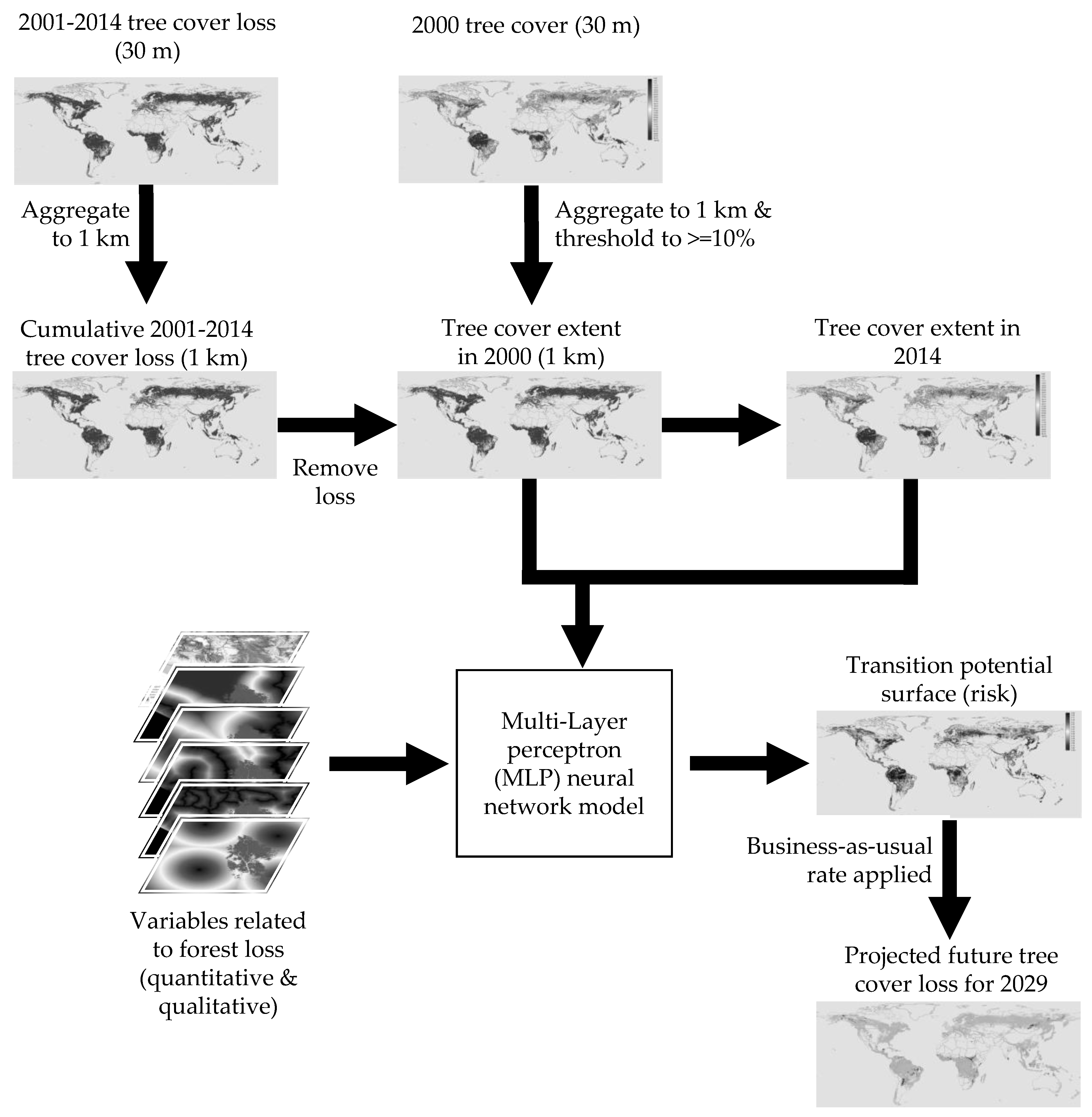
We used a suite of spatially-explicit global variables related to historical tree cover loss and an empirical modeling technique (the multi-layer perceptron neural network [23,24]) to combine the covariates of the variables with observed historical tree cover and tree cover loss data from 2000 to 2014 and assess the contribution of each variable to historical tree cover loss. This process yields transition potential surfaces that capture the potential of each pixel to transition from its current state. We then used the relationship between the variables and historical tree cover loss, captured in the transition potential surfaces, to generate 15-year projections of potential future tree cover loss for 2014–2029 under a BAU scenario.
2.1. Tree Cover Extent and Tree Cover Loss Data
We used a 30 m global map of percent tree cover in 2000 from [12] as the basis for this study and defined tree cover extent using a canopy cover threshold of 10% or more, following the FAO canopy cover definition for forest [25]. We aggregated the 30 m map of tree cover in 2000 to a 1 km map of tree cover to match the spatial resolution of many of the global variable data sources used in the study. We calculated the average percent tree cover of all 30 m pixels within each 1 km pixel, and then selected all 1 km pixels with 10% or more tree cover.
We defined tree cover loss as any change below the 10% threshold of tree cover. We used the 30 m global forest cover loss data for 2000–2014 from [12] and aggregated all loss from 2001–2014 to 1 km to create a map of tree cover loss from 2001–2014. Ref. [12] define loss as a “stand-replacement disturbance or the complete removal of tree canopy cover at the Landsat pixel”. We subtracted this loss map from the 1 km tree cover extent map for 2000 to create a tree cover extent and tree cover loss map for 2014 (Figure S1).
2.2. Variables Related to Forset Loss
We explored a wide range of 25 potential variables related to tree cover loss (Table 1) to fully capture the suite of variables that had been included in similar studies of deforestation at regional and national scales (e.g., [18,26,27]). The variables captured: (1) a variety of biophysical characteristics; (2) forest accessibility (based on distance to railroads, roads, trails, and airports); and (3) agricultural opportunity costs (distance to markets, economic rents for croplands, etc.). The variables included both quantitative variables (such as elevation and distance to roads) and qualitative variables (such as biomes and soil drainage). Quantitative variables were continuous and were included in the model directly without any transformation. Qualitative variables were categorical and were converted to normalized likelihoods prior to inclusion in the model. The normalized likelihood (NL) of a qualitative variable was calculated as:
where p(b|C) is the probability of change, i.e., tree cover loss, in a particularly class, or bin, and p(b|P) is the probability of persistence, i.e., tree cover persistence, in a particular class, or bin. Each NL was derived by calculating the proportion of pixels occurring within that class relative to the total size of the training sample for change or persistence.
2.3. Model Development and Projections
We generated one global model and six regional-scale models of tree cover loss. We calibrated each model based on observed historical tree cover loss and the covariates of the variables, and generated a transition potential surface for each model. The transition potential surface identifies the potential of each pixel to transition from its current state, in this study from tree cover to non-tree cover, thus highlighting areas of highest risk of tree cover loss; the transition potential surface provides the basis for identifying those pixels with the highest likelihood to change, or potential to transition. We used the transition potential surfaces as the basis to generate 15-year projections of potential future tree cover loss for 2014–2029 under a BAU scenario based on the historical deforestation rate (Figure 1). For both the global and regional scales of the analysis, we assessed the relationship between each of the 25 variables and the historical change (areas of tree cover loss between 2000 and 2014) and persistence (areas that remain under tree cover in 2014). We then selected the subset of variables that produced the highest model accuracy at each scale. We implemented all analyses at 1 km spatial resolution, reflecting the resolution of most of the variables and available computing capacity.
We tested the quantitative and qualitative variables, for both the global and regional analyses, against each other using regression and principal component analysis (PCA) to identify spatial autocorrelation, and assess explanatory power in predicting tree cover loss. The spatial autocorrelation tests eliminated three variables at the global scale: distance to airports, world population, and soil depth. We fed the remaining 22 variables in a multi-layer perceptron (MLP) neural network model [23,24] in the Land Change Modeler (LCM) in TerrSet software [28]. We selected the MLP because the MLP algorithm is less sensitive than other methods (such as logistical regression) to collinearity among independent variables and non-normal distributions [28]. MLP uses known areas of change, i.e., areas of historical tree cover loss, as training data to develop possible relationships between the input explanatory variables (e.g., distance to roads, slope, economic rent of croplands) and activation levels of the output nodes of the network [28]. MLP then uses additional known areas of change and persistence, or validation pixels, to validate the model. We used 25,000 pixels to train the model and 25,000 pixels to validate the model. MLP then calculates the expected model accuracy, and performs further validation and assessment of the resulting model through skill statistics for both change and persistence. Details of the equations are provided in the Appendix A. The skill statistic varies from −1 to +1; it is similar to the Heidke Skill Score and represents the skill score relative to a random forecast [29]. A skill of 0 means the model is doing better than chance, a skill of +1.0 indicates perfect prediction, and a negative skill indicates that the model is doing worse than by chance. Recognizing that the original variable datasets inherently contain errors, the MLP provides information regarding the importance of each variable in the development process and a skill score for the training process (which includes a subsample from each of the datasets). The MLP output also provides various statistics about the learning process. The statistics include the accuracy and skill with which the model predicted whether the validation pixels would remain tree cover, or change, resulting in tree cover loss. Among these are a set of sensitivity analyses performed to better understand the underlying structure of the model and the importance of each of the variables. Having fully trained the model using all variables, the MLP procedure performs these additional analyses, or tests. The first test evaluates the importance of each variable in the model by forcing a single variable to be constant and generating results using all other combinations (Table S1). A second sensitivity test, or evaluation, holds all variables except one constant; this test highlights interactions that exist among variables (Table S2). Lastly, a backwards elimination stepwise is performed to assess the impact of each variable on the overall accuracy of the model (Table S3). Beginning with the least influential variable in the model’s accuracy and skill, the next least influential variable is added, and additional variables sequentially added until only one variable, the most influential remains. This process informs the model development as it identifies those variables that did not significantly improve the overall accuracy of the model and can be permanently excluded [30,31]. The above sensitivity tests provide valuable information that the MLP use to generate the most parsimonious model. A parsimonious model aims to decrease complexity, improve efficiency, and reduce the likelihood of overfitting the model [29].
The global model results included a rank-ordered list of variables, based on their relative importance, and the final global model selected a subset based on this list to generate the global transition potential surface. The final global model in this study yielded a skill statistic of 0.61. We then used the final global model to generate a projection of potential future tree cover loss for 2029. In the projection process, the transition potential surface provides the basis for identifying those pixels with the highest preference to change, or potential to transition. We applied the historical global forest cover loss rate, derived from the [12] global forest cover loss data for 2000-2014, to the tree cover extent map in 2014, and assumed a BAU scenario. The historical global forest cover change rate, used for the BAU scenario, was calculated as 4.1%.
We repeated the modeling process for each of the six regions: Africa, Australia, Asia, Europe, North America, and South America (Figure S2), generating an independent MLP run for each region, and yielding six regional model results. The final regional models yielded skill statistics of 0.72, 0.59, 0.64, 0.53, 0.56, 0.83 for Africa, Australia, Asia, Europe, North America, and South America respectively. We then generated projections of potential future tree cover loss for 2029 for each of the regions, assuming a BAU scenario. We did this by applying the annual historical forest cover loss rates, derived from [12] to the tree cover extent map in 2014; the transition potential surfaces identified those pixels with the highest preference to change from tree to non-tree cover. The historical forest cover loss rates were 0.052 for Africa, 0.051 for Asia, 0.069 per year for Australia, 0.014 per year for Europe, 0.050 for North America, and 0.045 for South America.
3. Results
3.1. Explanatory Variables
The final global model included 15 variables that were significant in explaining tree cover loss. Table 2 lists the variables based on relative importance. The most important variables included precipitation, mean temperature, and crop suitability.
While the regional model results all included elevation, slope, aboveground biomass, crop suitability, mean temperature, precipitation, ecoregions and, at least one soil variable, regional differences were apparent (Table S4). For example, there were differences in the distance variables selected by the models, with distance to airports included in five of the models, but not in the model for Australia; distance to urban areas included in all models except Africa; and distance to roads included in four models, but not Asia or Africa. The model for South America did not include the human influence index, countries, or irrigation area—these three variables were present in the other regional models. Opportunity cost was only included in the models for South America and Europe; protected areas were an important variable in four of the models but not Asia or North America; and population in 2000 was only included in the models for Africa, Asia, and Europe.
3.2. Transition Potential Surface
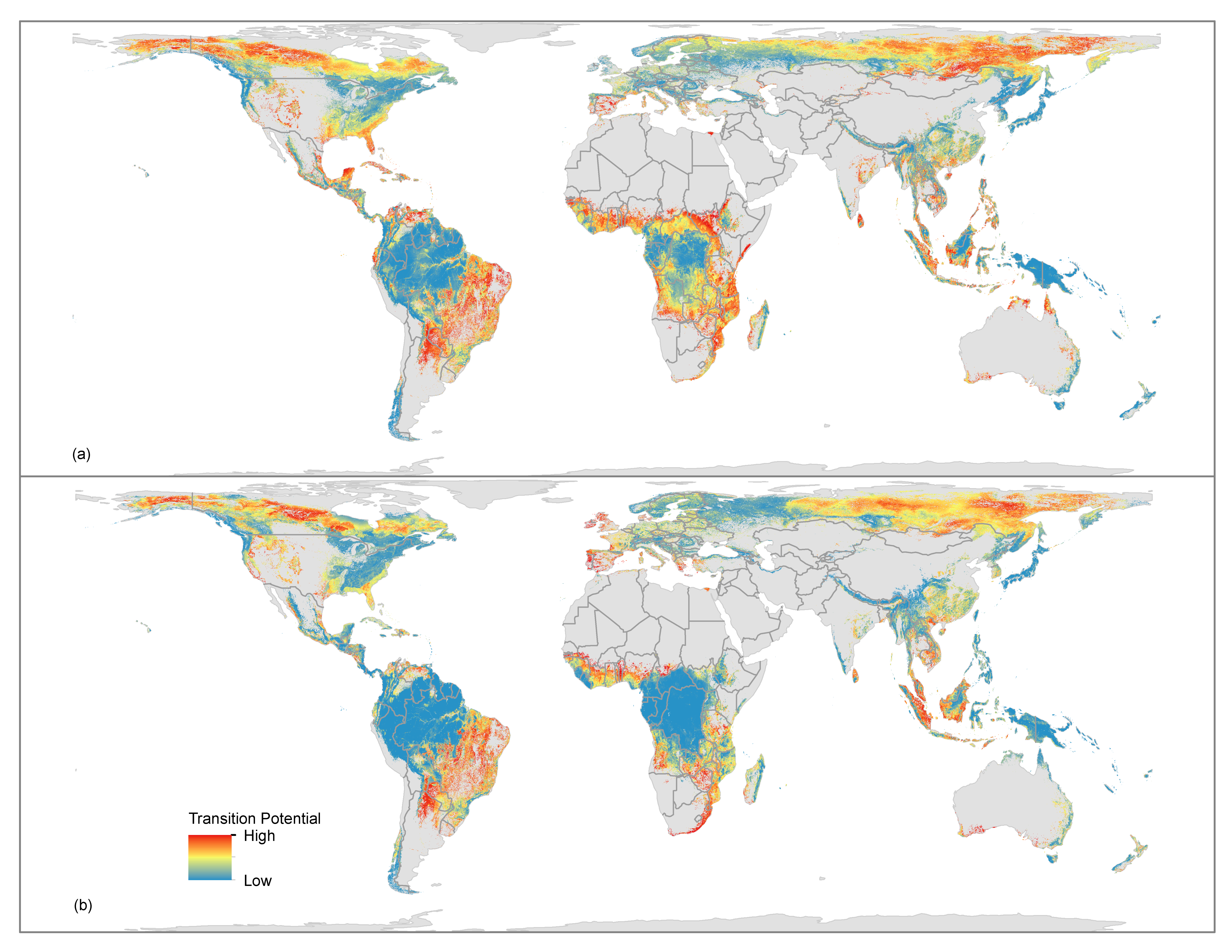
The global analysis revealed several major regions of high transition potential for tree cover loss in different biomes (Figure 2a). These included: (1) large areas of the boreal forest and taiga biome in Alaska, western Canada, and the eastern extents of Russia; (2) the temperate coniferous forests of the southeast United States; (3) the tropical and subtropical dry broadleaf forests in Mexico’s Yucatan Peninsula; (4) large swaths of the tropical and subtropical grasslands, savannas, and shrublands biome in South America, especially in Paraguay, Northern Argentina, and parts of Brazil; (5) large swaths of the subtropical grasslands, savannas, and shrublands biome in southern Sudan and Mozambique; and (6) the tropical and subtropical moist broadleaf forests in Sumatra, Indonesia. Four areas with a lower transition potential for tree cover loss were also revealed including: (1) the temperate broadleaf and mixed forest biome of the eastern United States and southeast Canada; (2) large swaths of the Amazon basin within the tropical and subtropical moist broadleaf forests biome of Brazil, Colombia, Peru, Suriname, and French Guiana; (3) areas of the tropical and subtropical moist broadleaf forests biome in the Congo Basin concentrated in the Democratic Republic of the Congo, the Republic of Congo, Gabon, and Cameroon; and (4) the tropical and subtropical moist broadleaf forests of New Guinea.
The transition potential surfaces generated for each of the six regions showed distinct patterns (Figure 2b). Most notably, the transition potential surface for North American illustrated a high transition potential in much of the boreal forest and taiga biome of northern Canada, interior Alaska, and central and eastern Russia. The transition potential surface for South America illustrated a high transition potential in areas of the tropical and subtropical grasslands, savannas, and shrublands biome in Brazil, Argentina, and Paraguay. Asia showed a high transition potential, particularly for Sumatra, in the tropical and subtropical moist broadleaf forests, but a low transition potential for the tropical and subtropical moist broadleaf forests in interior east and west Kalimantan. Other areas of low transition potential at the regional-level included: the boreal forest and taiga biome of western Russia, the temperate broadleaf and mixed forest biome of the eastern United States and southeast Canada, and much of the tropical and subtropical grasslands, savannas, and shrublands biome and tropical and subtropical moist broadleaf forests biome of the Congo Basin.
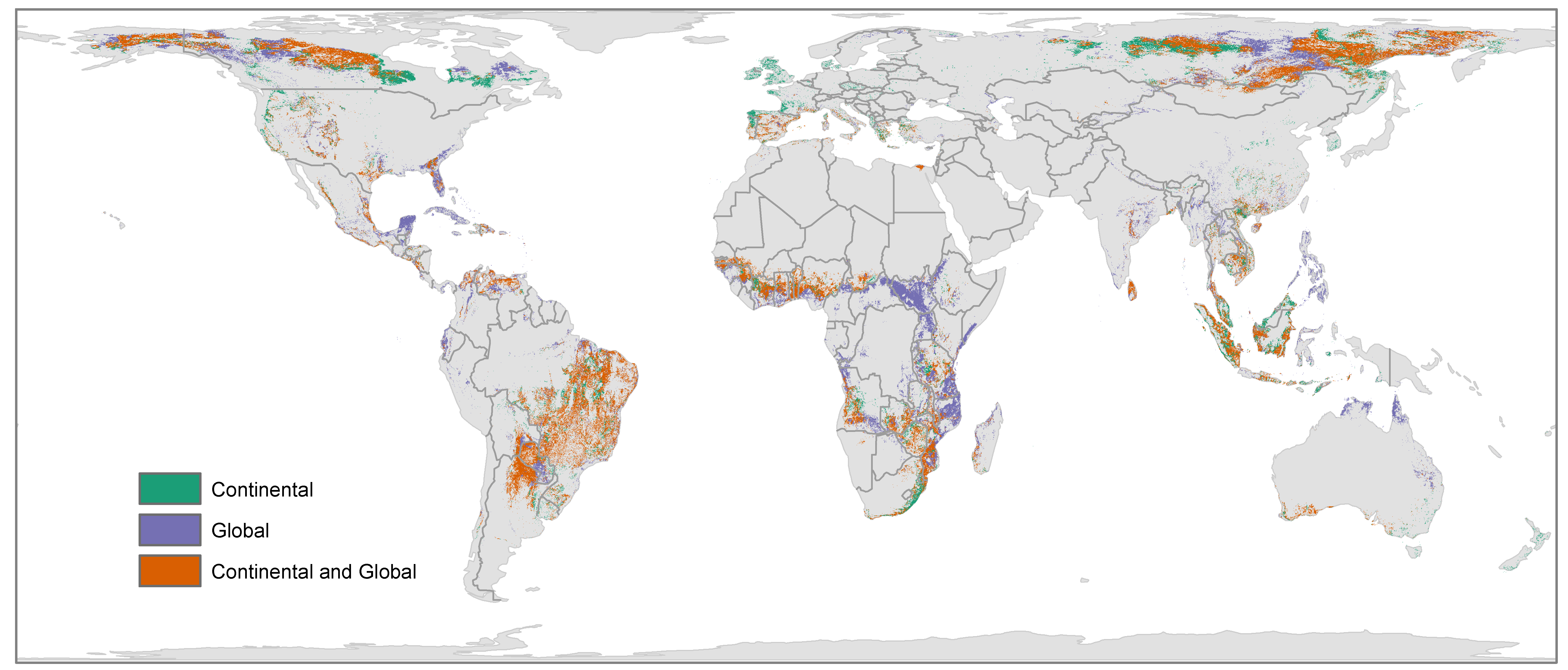
The global and regional results also revealed several areas of agreement in terms of a high risk of tree loss at both scales (Figure 3). These included: (1) the boreal forest and taiga regions of north central Canada, interior Alaska, and eastern Russia; (2) the tropical and subtropical grasslands, savannas, and shrublands of South America, covering northern Argentina, north western Paraguay, southeast Bolivia, and eastern Brazil; (3) the tropical and subtropical grasslands, savannas, and shrublands in parts of western and southeast Africa; and (4) the tropical and subtropical dry and moist broadleaf forests of southeast Asia including Sri Lanka, Cambodia, and parts of Indonesia. Differences also existed in the results across the two scales where, for example, either the global model or regional model produced a high transition potential and the other generated a low transition potential or vice versa. These included: (1) the boreal forest and taiga regions of north eastern and western Canada as well as central and western Russia; (2) the tropical & subtropical dry broadleaf forests, especially in Mexico; (3) the tropical and subtropical grasslands, savannas and shrublands in eastern Africa, especially southern Sudan, Tanzania, and Mozambique; and (3) the montane grasslands and shrublands, especially in South Africa.
3.3. Tree Cover Loss Projection Images
Based on our definition of tree cover as 10% or more canopy cover, and tree cover loss as any change below that threshold, we calculated that global tree cover loss was 4.1% between 2000 and 2014. Under a BAU scenario (i.e., assuming the same deforestation rates), our global model suggests another 4.4% of tree cover loss by 2029. Our global model results also suggest that several regions could experience increased tree cover loss between 2014 and 2029, most notably, South America, as well as areas of the subtropical moist broadleaf forests of Southern and Central Africa. Conversely, our results indicate that some areas that experienced significant tree cover loss between 2000 and 2014 could experience lower tree cover loss for the period 2014–2029. These include selected areas of the boreal forests/taiga biome in east central Russia and northern Canada, and the tropical and subtropical grasslands, savannas and shrublands of western Africa.
Based on our regional results, Europe exhibited the most stable tree cover extent between 2000 and 2014. Tree cover loss was only 1.8% during this period and, under a BAU scenario, our projections suggest Europe may experience an additional 2.1% tree cover loss between 2014 and 2029. Australia’s tree cover was reduced by 6.1% between 2000 and 2014 and could be reduced by an additional 6.5% between 2014 and 2029, under a BAU scenario. Similarly, tree cover in Africa was reduced by 5.1% between 2000 and 2014 and could contract an additional 5.3% between 2014 and 2029. In South America, tree cover loss was 4.6% between 2000 and 2014 and our results project an additional 4.9% tree cover loss between 2014 and 2029. In North America, tree cover loss was 3.9% between 2000 and 2014 and could increase to 4.7% between 2014 and 2029. In Asia, tree cover loss is projected to increase to 4.1% between 2014 and 2029 from 3.6% between 2000 and 2014.
4. Discussion
To our knowledge, our study has developed the first set of 1km maps showing the risk of tree cover loss and projections of potential future tree cover loss at both the global and regional scales based on models constructed using a series of spatially-explicit variables related to historical deforestation and globally-consistent data on historical tree cover and tree cover loss. The resolution of these maps takes advantage of the high-resolution tree cover loss data developed by [12] which inherently capture the finer scale patterns of tree cover loss. These new products are important for informing ongoing policy discussions about where forest conservation efforts are most urgently needed for biodiversity conservation, climate change mitigation, and achievement of the SDGs (e.g., [32,33]) as the maps highlight which areas are at greatest risk of tree cover loss as well as those areas projected to experience tree cover loss based on a 15-year BAU scenario. If combined with other global or regional datasets (such as data on carbon stocks, biodiversity, population growth), the outputs could inform where forest conservation would yield the greatest reductions in emissions from deforestation or bring the greatest synergies with biodiversity conservation or poverty alleviation [34]. Providing information on where tree cover loss is most likely could help governments focus their forest monitoring programs on the areas of greatest risk and set up near-real time alert systems (e.g., [35]) for quickly responding to deforestation. Providing information on areas with low tree cover loss risk could help inform the development of conservation incentives, such as payments for ecosystem services, aimed at preserving these low-risk areas. The models used to produce the maps also provide key information on the main variables associated with change at both the global and regional scale, thus helping to inform discussions on where to target efforts to address identified drivers of deforestation. For example, while the main driver of deforestation in many tropical regions includes agriculture (both subsistence and commercial [36], in boreal regions several studies have found that timber harvesting and wildfire dominate [37,38,39]. Providing information on the variables associated with tree cover loss allows policy makers, donors and practitioners to target their conservation funding, capacity-building, and efforts towards addressing specific drivers.
Our analysis provides novel insights into which forests are currently at greatest risk of being destroyed. It is clear that the risk of tree cover loss is non-uniform across regions and biomes. Our results suggest, for example, that areas in several biomes in South America are at risk including, for example, the tropical shrubland/savanna regions, especially northern Argentina and Paraguay. Areas of West and tropical Africa, and parts of the boreal and taiga region are also particularly at risk for losing tree cover. [37] found that two-thirds of the boreal forest biome is managed for wood production and industrial development and that resultant activities, most notably logging, are increasing. It is therefore reasonable to expect that tree cover loss may expand in this region. Identifying areas of highest risk of tree cover loss could help policymakers proactively develop innovative and anticipatory policies to prevent this loss.
Our projections of future tree cover loss, with an estimated 247 M ha of additional tree cover loss between 2014 and 2029 under a BAU scenario, indicate that tree cover loss will likely continue to occur at high rates unless significant action is taken. This figure for the 15 year period is almost two times greater than the estimated forest cover loss over the 25 year period from 1990–2015 [7]. Similar historical tree cover loss estimates calculated from GFW resulted in over 19 Gt of CO2 emissions for the period 2000–2014. While the global results highlight general vulnerability to change, the regional scale can identify areas more likely to change based on more localized pressures. Our regional results suggest that tree cover loss is projected to continue in all regions, however the greatest losses could occur in Asia (76 M ha), South America (56 M ha), and Africa (54 M ha). Other studies project similar patterns in some regions. Ref. [22] constructed deforestation projections through 2025 and 2050 and their results, while generated using coarse spatial resolution data, showed similar patterns of risk and areas of potential tree cover loss for tropical Africa and regions of South America. And, results from a study by [40] that generated deforestation projections for the period 2015 to 2030, also suggest similar patterns for South America.
Our results also highlight which variables associated with historical tree cover loss are most important at the global scale as well as which variables are regionally important. At the global scale, precipitation, mean temperature, and crop suitability were the most important variables. At the regional scale, similar to other studies [18,26,27], distance to roads, rail, airports, and trails proved important driver variables, thus highlighting the need to consider these variables in development and land use planning initiatives. The Global Forest Atlas [41] discusses the important role of transportation networks in increasing accessibility to remote forest areas, and how access to markets (presumably facilitated by distance to roads, rail, airports, etc.) further incentivizes commercial agriculture and forestry activities. Our results also identified novel variables at the regional scale, particularly AGB and the human influence index.
While we believe our data have utility for multiple policy and planning processes including biodiversity conservation, climate change mitigation, and sustainable development initiatives, several caveats exist. The development of fully-informed policies and planning activities also requires additional information (such as forest type, forest condition, forest governance issues, etc.). Our data provide one critical input for these activities by presenting robust and consistent information on the overall risk of forest loss, but other datasets are also needed. We also recognize that new (unanticipated) variables may become important in future years. For this study, we explored a comprehensive set of 25 variables and aimed to maximize consistency and ensure the variables would remain constant during the projection period by restricting the variables to the same period as the historical deforestation data and limiting the projection period to fifteen years. Further, the global nature of the variables, as well as the single tree cover threshold (10%) used in the study, make the results suitable for use in global and regional scale analyses; they have more limited utility in national and local scale analyses which require national driver information and national datasets [42,43,44]. We also used a global forest cover loss dataset that identifies loss irrelevant of management regime and, therefore, some loss occurrences may in fact reflect forestry rotation patterns. While we focused on tree cover loss in this study, future studies could incorporate, for example, tree cover gain data to assess the net carbon impacts of tree cover loss followed by reforestation. We also recognize that leakage is an important issue for forest conservation and, while beyond the focus of this study, future studies could assess this issue. We encourage others to pursue these needed research activities.
Recognizing the significant negative environmental, social and economic consequences of continued forest cover loss [1,5,44,45], our outputs highlight and reiterate the magnitude of the challenge and the urgent need to take action to quickly stem forest cover loss if the Aichi Targets, REDD+ initiative and SDG goals are to be achieved. Our outputs will also help inform the types of knowledge gaps identified by [46] regarding the interaction between habitat loss or degradation and climate change, as well as the need for improving understanding of climate-land interactions [47,31] and models, which rely on spatially- and temporally-explicit land cover data to predict climate responses.
5. Conclusions
Our study has produced the first robust, 1 km resolution, spatially consistent maps of tree cover loss risk using a series of spatially-explicit variables related to historical tree cover loss and globally consistent data on tree cover and historical tree cover loss. By combining historical these variables and historical tree cover loss information we identified areas where tree cover is at higher risk of future loss. We have also generated new projections of potential future global and regional tree cover loss by 2029, based on a BAU scenario. We have made all of the outputs fully available and have also highlighted the utility of these layers in multiple planning exercises and prioritization activities.
As the effects of climate change continue to manifest, and initiatives to combat deforestation are implemented, as part of climate change mitigation, biodiversity conservation, and the SDGs, the inclusion of these types of globally-consistent data should become standard practice. By including critical information on areas at high risk of tree cover loss in modeling and planning activities, more informed policy decisions will be possible that fully reflect the role of forests for biodiversity conservation, climate mitigation and sustainable development.
Supplementary Materials
The following are available online at https://0-www-mdpi-com.brum.beds.ac.uk/2073-445X/8/1/14/s1, Figure S1: 1 km tree cover extent and tree cover loss map for 2014, Figure S2: six regions used for the regional scale analyses, Table S1: Test performed in the Multi-Layer perceptron (MLP) neural network model process to evaluate the importance of each variable in the model by forcing a single independent variable to be constant and generating results using all other combinations, Table S2: Test performed in the Multi-Layer perceptron (MLP) neural network model process to highlight the interactions that exist among the variables by forcing all independent variables except one to be constant, Table S3: Backwards elimination stepwise test performed in the Multi-Layer perceptron (MLP) neural network model process to assess the impact of each variable on the overall accuracy of the model; example from the global model, Table S4: Driver variables (including both quantitative variables and the Normalized Likelihood (NL) of qualitative variables) for the six regional analyses, ordered by relative importance.
Author Contributions
Conceptualization, J.H., C.A.H., K.T., M.G.-R., and S.C.C.; Methodology, S.C.C., J.H., and M.G.-R.; Validation, S.C.C.; Writing—original draft preparation, J.H., S.C.C., and M.G.-R.; Writing—review and editing, J.H., C.A.H., S.C.C., K.T., and M.G.-R.
Funding
This work was partially funded by the Gordon and Betty Moore Foundation.
Acknowledgments
The authors thank Yashee Joshi and Tianze Li who both participated in the modeling activities. Tracy Hsin participated in a literature review and Kellee Koenig contributed to the generation of figures.
Conflicts of Interest
The authors declare no conflict of interest.
Appendix A
The expected model accuracy is a function of the number of transitions being modeled along with the number of persistence classes. The latter can be determined based on the number of “from” classes. The expected accuracy is:
where
E(A) = 1/(T + P)
- E(A) = expected accuracy;
- T = the number of transitions in the submodel;
- P = the number of persistence classes = the number of “from” classes in the sub-model.
A measure of the model skill is then expressed as:
where
S = (A − E(A))/(1 − E(A))
- S = model skill measure;
- A = measured accuracy;
- E(A) = expected accuracy.
This measure varies from −1 to +1 with a skill of 0 indicating random chance.
References
- Giam, X. Global biodiversity loss from tropical deforestation. Proc. Natl. Acad. Sci. USA 2017, 114, 5775–5777. [Google Scholar] [CrossRef] [PubMed] [Green Version]
- Commission on Genetic Resources for food and Agriculture, FAO. State of the World’s Forest Genetic Resources. 2014. Available online: http://www.fao.org/3/a-i3825e.pdf (accessed on 19 October 2018).
- Restrepo, J.D.; Kettner, A.J.; Syvitski, J.P.M. Recent deforestation causes rapid increase in river sediment load in the Colombian Andes. Anthropocene 2015, 10, 13–28. [Google Scholar] [CrossRef]
- Van der Werf, G.R.; Morton, D.C.; DeFries, R.S.; Olivier, J.G.; Kasibhatla, P.S.; Jackson, R.B.; Collatz, G.J.; Randerson, J.T. CO2 Emissions from Forest Loss. Nat. Geosci. 2009, 11, 737–738. [Google Scholar] [CrossRef]
- Baccini, A.; Goetz, S.J.; Walker, W.S.; Laporte, N.T.; Sun, M.; Sulla-Menashe, D.; Hackler, J.; Beck, P.S.A.; Dubayah, R.; Friedl, M.A.; et al. Estimated carbon dioxide emissions from tropical deforestation improved by carbon-density maps. Nat. Clim. Chang. 2012, 2, 182–185. [Google Scholar] [CrossRef]
- Harris, N.L.; Brown, S.; Hagen, S.C.; Saatchi, S.S.; Petrova, S.; Salas, W.; Hansen, M.C.; Potapov, P.V.; Lotsch, A. Baseline Map of Carbon Emissions from Deforestation in Tropical Regions. Science 2012, 336, 1573–1576. [Google Scholar] [CrossRef] [PubMed]
- Keenan, R.J.; Reams, G.A.; Achard, F.; de Freitas, J.V.; Grainger, A.; Lindquist, E. Dynamics of global forest area: Results from the FAO Global Forest Resources Assessment 2015. For. Ecol. Manag. 2015, 352, 9–20. [Google Scholar] [CrossRef] [Green Version]
- Tropical Forest Alliance 2020. Available online: https://www.tfa2020.org/en/ (accessed on 19 October 2018).
- Congo Basin Forest Fund-African Development Bank. Available online: https://www.afdb.org/en/topics-and-sectors/initiatives-partnerships/congo-basin-forest-fund/ (accessed on 19 October 2018).
- Amazon Fund. Available online: http://www.amazonfund.gov.br/en/home/ (accessed on 19 October 2018).
- Sandel, B.; Svenning, J.-C. Human impacts drive a global topographic signature in tree cover. Nat. Commun. 2013, 4, 2474. [Google Scholar] [CrossRef] [Green Version]
- Hansen, M.C.; Potapov, P.V.; Moore, R.; Hancher, M.; Turubanova, S.A.; Tyukavina, A.; Thau, D.; Stehman, S.V.; Goetz, S.J.; Loveland, T.R.; et al. High-Resolution Global Maps of 21st-Century Forest Cover Change. Science 2013, 342, 850–853. [Google Scholar] [CrossRef]
- Kim, D.-H.; Sexton, J.O.; Noojipady, P.; Huang, C.; Anand, A.; Channan, S.; Feng, M.; Townshend, J.R. Landsat-based forest-cover change from 1990 to 2000. Remote Sens. Environ. 2014, 155, 178–193. [Google Scholar] [CrossRef]
- Achard, F.; House, J.I. Reporting carbon losses from tropical deforestation with Pan-tropical biomass maps. Environ. Res. Lett. 2015, 10, 101002. [Google Scholar] [CrossRef] [Green Version]
- Song, X.-P.; Huang, C.; Saatchi, S.S.; Hansen, M.C.; Townshend, J.R. Annual Carbon Emissions from Deforestation in the Amazon Basin between 2000 and 2010. PLoS ONE 2015, 10, e0126754. [Google Scholar] [CrossRef] [PubMed]
- Southworth, J.; Marsik, M.; Qiu, Y.; Perz, S.; Cumming, G.; Stevens, F.; Rocha, K.; Duchelle, A.; Barnes, G. Roads as Drivers of Change: Trajectories across the Tri‑National Frontier in MAP, the Southwestern Amazon. Remote Sens. 2011, 3, 1047–1066. [Google Scholar] [CrossRef] [Green Version]
- Pérez-Vega, A.; Mas, J.-F.; Ligmann-Zielinska, A. Comparing two approaches to land use/cover change modeling and their implications for the assessment of biodiversity loss in a deciduous tropical forest. Environ. Model. Softw. 2012, 29, 11–23. [Google Scholar] [CrossRef]
- Fuller, D.O.; Hardiono, M.; Meijaard, E. Deforestation Projections for Carbon-Rich Peat Swamp Forests of Central Kalimantan, Indonesia. Environ. Manag. 2011, 48, 436–447. [Google Scholar] [CrossRef]
- Vieilledent, G.; Grinand, C.; Vaudry, R. Forecasting deforestation and carbon emissions in tropical developing countries facing demographic expansion: A case study in Madagascar. Ecol. Evol. 2013, 3, 1702–1716. [Google Scholar] [CrossRef] [PubMed]
- Cramer, W.; Bondeau, A.; Schaphoff, S.; Lucht, W.; Smith, B.; Sitch, S. Tropical forests and the global carbon cycle: Impacts of atmospheric carbon dioxide, climate change and rate of deforestation. Philos. Trans. R. Soc. B Biol. Sci. 2004, 359, 331–343. [Google Scholar] [CrossRef]
- Tracewski, Ł.; Butchart, S.H.M.; Donald, P.F.; Evans, M.; Fishpool, L.D.C.; Buchanan, G.M. Patterns of twenty-first century forest loss across a global network of important sites for biodiversity. Remote Sens. Ecol. Conserv. 2016, 2, 37–44. [Google Scholar] [CrossRef]
- Pahari, K.; Murai, S. Modelling for Prediction of Global Deforestation Based on the Growth of Human Population. Available online: http://paper/Modelling-for-prediction-of-global-deforestation-on-Pahari-Murai/0e29acd1426cd542f0a45de1211d303d8865ca09 (accessed on 19 October 2018).
- Yeh, A.G.-O.; Li, X. Urban simulation using neural networks and cellular automata for land use planning. In Advances in Spatial Data Handling; Richardson, D.D.E., van Oosterom, P.D.P., Eds.; Springer: Berlin/Heidelberg, Germany, 2002; pp. 451–464. ISBN 978-3-642-62859-7. [Google Scholar]
- Pijanowski, B.C.; Brown, D.G.; Shellito, B.A.; Manik, G.A. Using neural networks and GIS to forecast land use changes: A Land Transformation Model. Comput. Environ. Urban Syst. 2002, 26, 553–575. [Google Scholar] [CrossRef]
- FAO. FRA 2015 Terms and Definitions. Forest Resources Assessment Working Paper 180. Available online: http://www.fao.org/docrep/017/ap862e/ap862e00.pdf (accessed on 15 March 2018).
- Sangermano, F.; Toledano, J.; Eastman, J.R. Land cover change in the Bolivian Amazon and its implications for REDD+ and endemic biodiversity. Landsc. Ecol. 2012, 27, 571–584. [Google Scholar] [CrossRef]
- Sudhakar Reddy, C.; Saranya, K.R.L. Earth observation data for assessment of nationwide land cover and long-term deforestation in Afghanistan. Glob. Planet. Chang. 2017, 155, 155–164. [Google Scholar] [CrossRef]
- Eastman, J.R.; Toledano, J. A short presentation of the Land Change Modeler (LCM). In Geomatic Approaches for Modeling Land Change Scenarios; Camacho Olmedo, T.M., Paegelow, M., Mas, J.-F., Escobar, F., Eds.; Lecture Notes in Geoinformation and Cartography; Springer: New York, NY, USA, 2018; pp. 499–505. ISBN 978-3-319-60801-3. [Google Scholar]
- Potts, J.M. Basic concepts. In Forecast Verification; Jolliffe, I.T., Stephenson, D.B., Eds.; John Wiley & Sons, Ltd.: Chichester, UK, 2012; pp. 11–29. ISBN 978-1-119-96000-3. [Google Scholar]
- Saifullah, K.; Barus, B.; Rustiadi, E. Spatial modelling of land use/cover change (LUCC) in South Tangerang City, Banten. IOP Conf. Ser. Earth Environ. Sci. 2017, 54, 012018. [Google Scholar] [CrossRef] [Green Version]
- Tompkins, A.M.; Caporaso, L.; Biondi, R.; Bell, J.P. A Generalized Deforestation and Land-Use Change Scenario Generator for Use in Climate Modelling Studies. PLoS ONE 2015, 10, e0136154. [Google Scholar] [CrossRef] [PubMed]
- Mackey, B.; DellaSala, D.A.; Kormos, C.; Lindenmayer, D.; Kumpel, N.; Zimmerman, B.; Hugh, S.; Young, V.; Foley, S.; Arsenis, K.; et al. Policy Options for the World’s Primary Forests in Multilateral Environmental Agreements. Conserv. Lett. 2014, 8, 139–147. [Google Scholar] [CrossRef]
- Swamy, L.; Drazen, E.; Johnson, W.R.; Bukoski, J.J. The future of tropical forests under the United Nations Sustainable Development Goals. J. Sustain. For. 2017, 37, 221–256. [Google Scholar] [CrossRef] [Green Version]
- Sunderlin, W.D.; Angelsen, A.; Belcher, B.; Burgers, P.; Nasi, R.; Santoso, L.; Wunder, S.; Sunderlin, W.D.; Angelsen, A.; Belcher, B.; et al. Livelihoods, forests, and conservation in developing countries: An Overview. World Dev. 2005, 33, 1383–1402. [Google Scholar] [CrossRef]
- Musinsky, J.; Tabor, K.; Cano, C.A.; Ledezma, J.C.; Mendoza, E.; Rasolohery, A.; Sajudin, E.R. Conservation impacts of a near real-time forest monitoring and alert system for the tropics. Remote Sens. Ecol. Conserv. 2018. [Google Scholar] [CrossRef] [Green Version]
- Curtis, P.G.; Slay, C.M.; Harris, N.L.; Tyukavina, A.; Hansen, M.C. Classifying Drivers of Global Forest Loss. Science 2018, 361, 1108–1111. [Google Scholar] [CrossRef]
- Gauthier, S.; Bernier, P.; Kuuluvainen, T.; Shvidenko, A.Z.; Schepaschenko, D.G. Boreal forest health and global change. Science 2015, 349, 819–822. [Google Scholar] [CrossRef] [PubMed]
- Potapov, P.V.; Turubanova, S.A.; Tyukavina, A.; Krylov, A.M.; McCarty, J.L.; Radeloff, V.C.; Hansen, M.C. Eastern Europe’s Forest Cover Dynamics from 1985 to 2012 Quantified from the Full Landsat Archive. Remote Sens. Environ. 2015, 159, 28–43. [Google Scholar] [CrossRef]
- Li, Z.; Deng, X.; Shi, O.; Ke, X.; Liu, Y. Modeling the Impacts of Boreal Deforestation on the Near-Surface Temperature in European Russia. Adv. Meteorol. 2013, 1–9. [Google Scholar] [CrossRef]
- d’Annunzio, R.; Sandker, M.; Finegold, Y.; Min, Z. Projecting global forest area towards 2030. For. Ecol. Manag. 2015, 352, 124–133. [Google Scholar] [CrossRef] [Green Version]
- Global Forest Atlas|Roads & Forests. Available online: https://globalforestatlas.yale.edu/land-use/infrastructure/roads-forests (accessed on 19 October 2018).
- Hosonuma, N.; Herold, M.; De Sy, V.; De Fries, R.S.; Brockhaus, M.; Verchot, L.; Angelsen, A.; Romijn, E. An assessment of deforestation and forest degradation drivers in developing countries. Environ. Res. Lett. 2012, 7, 044009. [Google Scholar] [CrossRef] [Green Version]
- Kissinger, G.; Herold, M.; de Sy, V. Drivers of Deforestation and Forest Degradation: A Synthesis Report for REDD+ Policymakers; Lexeme Consulting: Vancouver, BC, Canada, 2012. [Google Scholar]
- Salvini, G.; Herold, M.; De Sy, V.; Kissinger, G.; Brockhaus, M.; Skutsch, M. How countries link REDD+ interventions to drivers in their readiness plans: Implications for monitoring systems. Environ. Res. Lett. 2014, 9, 074004. [Google Scholar] [CrossRef]
- Newbold, T.; Hudson, L.N.; Hill, S.L.L.; Contu, S.; Lysenko, I.; Senior, R.A.; Börger, L.; Bennett, D.J.; Choimes, A.; Collen, B.; et al. Global effects of land use on local terrestrial biodiversity. Nature 2015, 520, 45–50. [Google Scholar] [CrossRef] [PubMed] [Green Version]
- Segan, D.B.; Murray, K.A.; Watson, J.E.M. A global assessment of current and future biodiversity vulnerability to habitat loss–climate change interactions. Glob. Ecol. Conserv. 2016, 5, 12–21. [Google Scholar] [CrossRef] [Green Version]
- Lawrence, D.; Vandecar, K. Effects of tropical deforestation on climate and agriculture. Nat. Clim. Chang. 2015, 5, 27–36. [Google Scholar] [CrossRef]
Figure 1.
Flow diagram of the steps used to generate the transition potential surface and potential future tree cover loss for 2029 at the global scale. (A similar process was used for each of the six regional models).
Figure 1.
Flow diagram of the steps used to generate the transition potential surface and potential future tree cover loss for 2029 at the global scale. (A similar process was used for each of the six regional models).

Figure 2.
Results for the Global model (a) and Regional models (b) (displayed together) showing areas of high potential to transition from tree cover to tree cover loss (red) to areas of low potential to transition (blue).
Figure 2.
Results for the Global model (a) and Regional models (b) (displayed together) showing areas of high potential to transition from tree cover to tree cover loss (red) to areas of low potential to transition (blue).

Figure 3.
Areas of high transition potential (i.e., high risk of tree cover loss) in the global or regional model results, or both.
Figure 3.
Areas of high transition potential (i.e., high risk of tree cover loss) in the global or regional model results, or both.


Table 1.
Initial set of variables (and data sources) considered for inclusion in the models at both scales, including; quantitative (1–15) and qualitative variables (16–25).
Table 1.
Initial set of variables (and data sources) considered for inclusion in the models at both scales, including; quantitative (1–15) and qualitative variables (16–25).
| Variable | Source | |
|---|---|---|
| 1 | Distance to railroads | VMap0 (Esri) |
| 2 | Distance to roads | VMap0 (Esri) |
| 3 | Distance to trails | VMap0 (Esri) |
| 4 | Distance to Airports | VMap0 (Esri) |
| 5 | Distance to urban areas | Nelson (2008). Estimated travel time to the nearest city of 50,000 or more people in year 2000 |
| 6 | Elevation | Danielson and Gesch (2011). Global Multi-resolution Terrain Elevation Data (GMTED2010) |
| 7 | Slope | Derived from Elevation |
| 8 | Aboveground Biomass | Avitabile et al. (2016). GEOCARBON global aboveground forest biomass map |
| 9 | Human Influence Index | Wildlife Conservation Society et al. (2005). Global Human Influence Index Dataset of the Last of the Wild Project generated at 1km for the period 1995–2004 by the World Conservation Society and the Columbia University Center for International Earth Science Information Network (CIESIN). |
| 10 | Crop suitability | Zabel et al. (2014). Global Assessment of Land Use Dynamics, Greenhouse Gas Emissions and Ecosystem Services (GLUES) data agricultural suitability data |
| 11 | Irrigation area | Siebert et al. (2013). FAO Irrigation Dataset |
| 12 | World Population 2000 | CIESIN (2016). World population in 2000 from NASA’s Socioeconomic Data and Application Center (SEDAC) |
| 13 | Global Opportunity Cost | Naidoo and Iwamura (2007). Global-scale mapping of economic benefits from agricultural lands: Implications for conservation priorities |
| 14 | Annual Precipitation | Hijmans et al. (2005). Average monthly precipitation in mm at a spatial resolution of 2.5 m from the WorldClim dataset |
| 15 | Annual Mean temperature | Hijmans et al. (2005). Average monthly mean temperature in in °C (×10) at a spatial resolution of 2.5 m from the WorldClim dataset |
| 16 | Protected Areas—Normalized Likelihoods | WDPA (2016). World Database on Protected Areas |
| 17 | Ecoregions—Normalized Likelihoods | WWF (2004). World Wildlife Fund—Global 200 (terrestrial) Ecoregions |
| 18 | Biomes—Normalized Likelihoods | WWF (2004). World Wildlife Fund—Global 200 (terrestrial) Ecoregions |
| 19 | Soil Depth—Normalized Likelihoods | HWSD (2014). Harmonized World Soil Database, version 1.2 |
| 20 | Soil Drainage—Normalized Likelihoods | HWSD (2014). Harmonized World Soil Database, version 1.2 |
| 21 | Soil Texture—Normalized Likelihoods | HWSD (2014). Harmonized World Soil Database, version 1.2 |
| 22 | Soil pH—Normalized Likelihoods | HWSD (2014). Harmonized World Soil Database, version 1.2 |
| 23 | Regions—Normalized Likelihoods | VMap0 (Esri) |
| 24 | Countries—Normalized Likelihoods | VMap0 (Esri) |
| 25 | States & Provinces—Normalized Likelihoods | VMap0 (Esri) |
Table 2.
Variable results for the global analysis, ranked by relative importance to the model accuracy.
Table 2.
Variable results for the global analysis, ranked by relative importance to the model accuracy.
| Variable | Relative Importance |
|---|---|
| Precipitation | 1 |
| Mean temperature | 2 |
| Crop suitability | 3 |
| Biomes (NL) | 4 |
| AGB | 5 |
| Elevation | 6 |
| Slope | 7 |
| Irrigation area | 8 |
| Distance to roads | 9 |
| Distance to railroads | 10 |
| Distance to trails | 11 |
| Human Influence Index | 12 |
| Distance to urban areas | 13 |
| Opportunity Cost | 14 |
| Protected areas (NL) | 15 |
© 2019 by the authors. Licensee MDPI, Basel, Switzerland. This article is an open access article distributed under the terms and conditions of the Creative Commons Attribution (CC BY) license (http://creativecommons.org/licenses/by/4.0/).
Share and Cite
MDPI and ACS Style
Hewson, J.; Crema, S.C.; González-Roglich, M.; Tabor, K.; Harvey, C.A. New 1 km Resolution Datasets of Global and Regional Risks of Tree Cover Loss. Land 2019, 8, 14. https://0-doi-org.brum.beds.ac.uk/10.3390/land8010014
AMA Style
Hewson J, Crema SC, González-Roglich M, Tabor K, Harvey CA. New 1 km Resolution Datasets of Global and Regional Risks of Tree Cover Loss. Land. 2019; 8(1):14. https://0-doi-org.brum.beds.ac.uk/10.3390/land8010014
Chicago/Turabian StyleHewson, Jennifer, Stefano C. Crema, Mariano González-Roglich, Karyn Tabor, and Celia A. Harvey. 2019. "New 1 km Resolution Datasets of Global and Regional Risks of Tree Cover Loss" Land 8, no. 1: 14. https://0-doi-org.brum.beds.ac.uk/10.3390/land8010014
Note that from the first issue of 2016, this journal uses article numbers instead of page numbers. See further details here.