Article

Temporal Variation in Preferential Water Flow during Natural Vegetation Restoration on Abandoned Farmland in the Loess Plateau of China

School of Geography and Tourism, Shaanxi Normal University, Xi’an 710119, China
*
Author to whom correspondence should be addressed.
Submission received: 12 November 2019 / Revised: 3 December 2019 / Accepted: 5 December 2019 / Published: 6 December 2019
(This article belongs to the Special Issue Soil Erosion Processes and Rates in Arid and Semiarid Ecosystems)

Abstract

:
The restoration of vegetation in abandoned farmlands is an effective approach to control soil erosion on the Chinese Loess Plateau. However, few studies have investigated the effect of natural restoration age on the infiltration patterns and preferential flow in soil layers. This study examined the effect of the temporal variations in the degree of preferential flow and their contribution on the total infiltration in abandoned farmlands restored with different vegetation communities. In total, four sites were investigated, namely site AF3, AF12, AF18 and AF25 of restoration age of 3, 12, 18 and 25 years, respectively. A traditional dye tracer experiment was adopted to visualize the water flow behavior in the four sites. A semi-variance analysis was conducted to interpret the spatial variability of the soil water induced by infiltration. The results showed that both the soil properties and the root systems improved with the increased natural restoration ages combined with the effect of the plant species. The degree of preferential flow from the lowest to the highest occurred in AF3, AF12, AF18 and AF25, which was mainly affected by the development of root systems. Also, the abundant lateral root and steeper slope may have caused the presence of lateral flow in AF18 and AF25. Meanwhile, the spatial variability of the soil water in the infiltration patterns through vertical soil profiles increased from AF3 to AF25. Compared to AF3, the infiltration volume through preferential pathways in AF12, AF18 and AF25 increased by 1.73 times, 1.94 times and 4.09 times, respectively. Therefore, the preferential flow was improved in abandoned farmland in the presence of natural vegetation restoration that can increase water storage in the deep soil layer and reduce surface runoff and erosion.

1. Introduction

The Chinese Loess Plateau has suffered from severe soil erosion for several decades. The average annual erosion rates generally range between 5000 and 10,000 t/km2/a because of the intensive human disturbance and the presence of a thick erodible soil [1]. The impact of human activities in the plateau can be attributed to continuous and widespread stress, such as large-scale monocultures (wheat and maize) and over-grazing [2]. To control soil erosion and ecosystem degradation, the Chinese government initiated the “Grain-for-Green” project across the country in 1998. As important management of the project, vast areas of farmland in the Loess Plateau have been abandoned and converted into grasslands, shrublands or forests with natural vegetation [3]. Consequently, the soil loss of the plateau decreased by 57% and the vegetation cover increased by 13 times since 1998 [4,5]. The dense vegetation restoration activities and the increasing vegetation cover require a greater amount of water to survive [6]. However, water is usually scarce in the Loess Plateau, where the precipitation is low, the evapotranspiration is high, and the groundwater is deep [7]. Therefore, understanding the responses of the hydrological process to vegetation restoration in abandoned farmlands is essential for estimating their sustainable development.
Infiltration is a key component for storing water in soil layers within the hydrological process [8]. Soil water infiltration involves matrix flow and preferential flow [9]. Matrix flow represents the slow and even movement of water and solutes through the bulk soil [10], while preferential flow refers to the quick flow of water through the soil macrospores that bypasses most of the soil matrix [11]. At a soil profile, cracks, fissures, voids, fauna activities and root channels form a complex network that offers the ideal preferential pathways for water movement [12]. Through the preferential pathways, water and solutes can move to far greater depths than those predicted through the Richards’ equation [13]. As a result, the preferential flow could noticeably increase soil water conservation and groundwater recharge [14]. Dye tracer experiments are valuable techniques for visualising preferential water flow pathways [15]. Quantitative studies on preferential infiltration volume and its contribution to total infiltration and water storage remain nonetheless very limited.
Experiential evidence from field studies suggested that preferential flow processes varied considerably from one site to another [16]. Preferential water flow behaviour is primarily influenced by the soil properties, the rock fragments, the faunal activities, and the plant root systems [12,17,18]. With increasing abandonment time, the soil physical and chemical characteristics, the vegetation species and the plant root system in farmland can change significantly. Previous studies have confirmed that farmlands undergo significant increase in soil total porosity, soil organic matter content [19], soil clay content [20], total nitrogen [21] and aggregate stability [2] after a period of abandonment. Once farmland is abandoned, the vegetation recovers into tall herb, shrub, or forest ecosystems [3]. The plant species diversities and the plant communities vary greatly during the succession process [6]. The root system is the fundamental part of vegetation, and its mass density increases with the abandonment time [20]. Also, roots of different plant species, with diverse morphology, traits and distribution in soil layers tend to be vitally important for shaping the soil structure and the development from the soil surface to subsurface [22]. Those changes stimulated by the abandonment time certainly influence the soil hydrological properties and the water flow behavior. However, few studies have been conducted to investigate the temporal variations in the preferential flow of different vegetation communities after farmland abandonment.
Meanwhile, water flow moves into the soil layers through preferential pathways, which lead to the heterogeneity in the soil water through the soil profile [23]. Geostatistical methods were not only used to reveal the spatial variation of the soil water at slope and watershed scale but also at centimeter scale [24]. In this study, we investigate the vertical water flow behavior and the preferential infiltration based on a dye tracer experiment at four farmlands with different abandonment time and vegetation community. The aims of this study were threefold: (1) to identify the temporal variations in the soil properties and the root systems, and their relationship with the preferential flow with natural restoration age; (2) to contrast the water flow behavior in the soil profiles of the four abandoned farmland; (3) to assess the contribution of the preferential infiltration to the soil water storage during vegetation restoration.

2. Materials and Methods
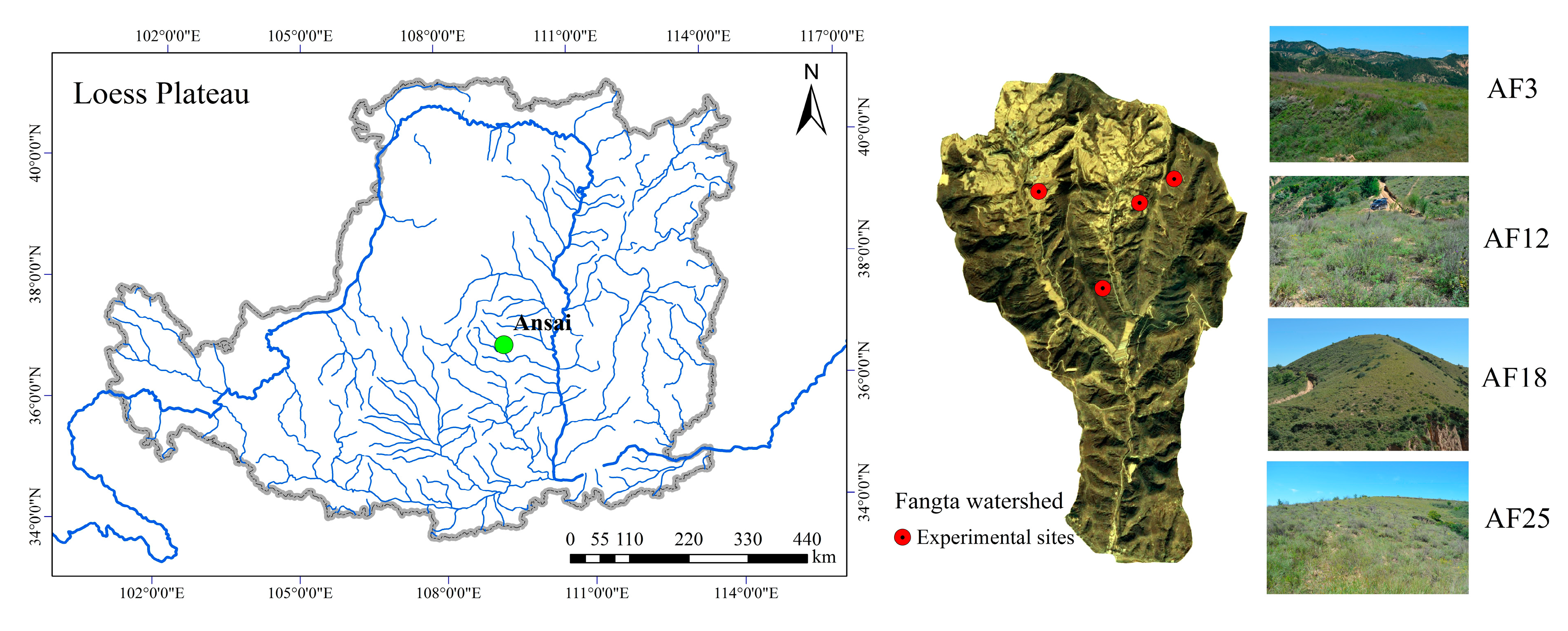
2.1. Study Area

The study site was located in the Fangta catchment (36°46′13″–36°49′18″ N, 109°15′22″–109°17′01″ E) in the An’sai County of the Shaanxi Province, in North China (Figure 1). This region is representative of the loess hill and the gully region of the Loess Plateau. It has a semi-arid continental climate with a mean annual temperature of 8.8 °C, and mean annual precipitation of 505 mm, over 70% of which occurs from July to September [20]. Soils in this watershed mainly are red Loess (the Early or Mid-Pleistocene Loess) and yellow loess (the Late Plesitocene Loess). According to the World Reference Base for soil Resource (WRB), yellow Loess soil was classified as Calcaric Regosols and red Loess soil belonged to Calcaric/Chromic Cambisols. The dominated plant communities are composed of artificial forest and shrubs (Robinia pseudoacacia, Caragana korshinski and Hippophae rhamnoides), natural shrubs (Rosa xanthine and Sophora davidii), natural grasses (A. gmelinii, Stipa bungeana, Bothriochloa ischaemum, A. giraldii and Lespedeza davurica). Following the “Grain to Green” project, a significant portion of the steep farmland area in this region was converted to forestland or grassland.

2.2. Experimental Design

After a detailed field survey and several interviews with the residents, four abandoned farmlands with respective abandonment times of 3, 12, 18 and 25 years were selected in this study (Table 1). The four sites were covered by different plant communities of Artemisia scoparia, Artemisia sacrorum, Bothriochloa ischaemum and Periploca sepium Bunge, representing the succession sequence of the natural vegetation in this area [6]. The terrain, the soil type and the previous tillage practices of these four abandoned farmlands are similar except for their plant communities and their respective abandonment time. In each test site, three plots at the middle slope were selected as replicates. The selected plots were located at least 3 m apart to avoid interference. From July to August 2018, all the experiments were conducted on these four sites. Soil and plant root sampling, as well as dye tracer experiments, were completed in the fields where rainfall had not occurred for five days.

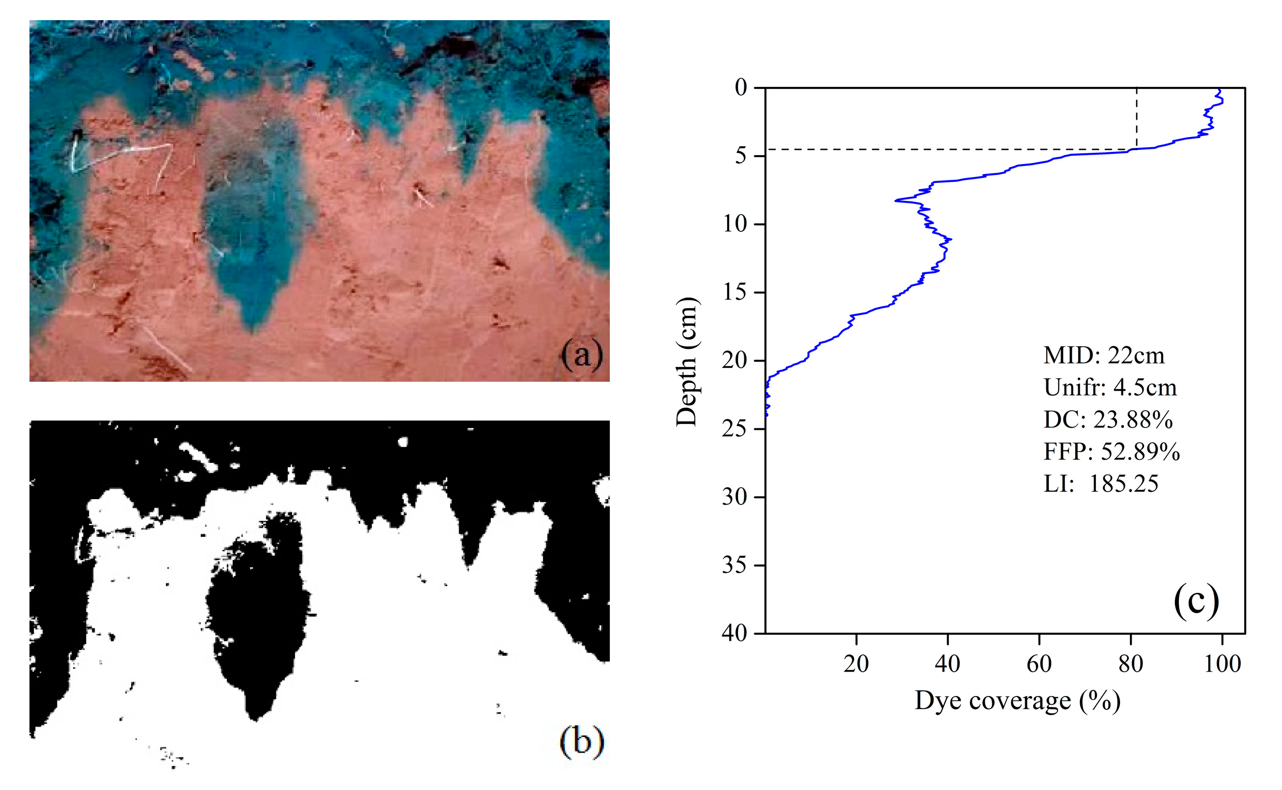
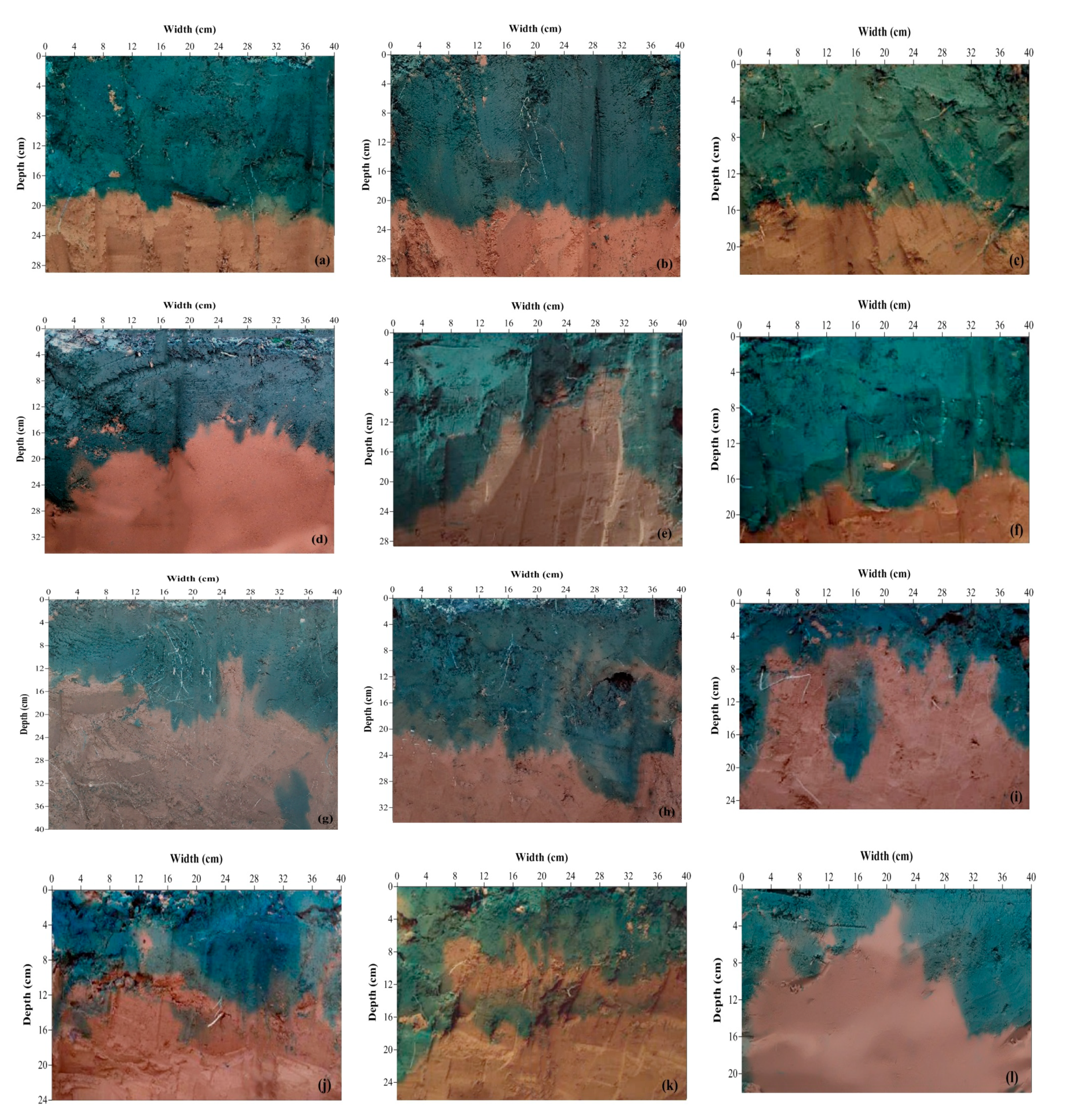
2.3. Dye-Tracer Experiment

Twelve dye-tracer experiments were conducted in the four test sites (four sites × three plot replications). In each plot, one hollow stainless-steel cube (length: 0.4 m; width: 0.4 m; height: 0.4 m) was inserted into the soil at 10–15 cm depth by using a rubber hammer. The aboveground plants were clipped to ground level and litter were removed carefully before the application of the dye tracer. The 12 plots were all irrigated with 10 L tap water which was dyed with Brilliant Blue FCF at a concentration of 4 g/L [24]. The falling head method was used to measure the soil infiltration process [5]. After irrigation, the surface of the stainless-steel cube was covered by plastic sheeting to prevent rainfall and evaporation. Twenty-four hours after the end of the infiltration, the plastic sheeting and the cube were removed carefully. The vertical soil profiles (width: 0.6 m; depth: 0.6 m) were excavated at the center of the cube. The dyed soil profiles were photographed using a digital camera (AF-S D5600, Nikon, Tokyo, Japan) under daylight conditions.
Soil sampling was conducted after the images were obtained through subdividing the profile into small grids of 2 × 2 cm (width × height) to extract soil samples with a volume of 4 cm3 (width × height × thickness: 2 × 2 × 1 cm), following the procedures thoroughly detailed by Mei et al. [24]. A total of 400 soil samples for each profile (width: 40 cm; depth: 40 cm) were dried at 105 °C for 24 h to measure the gravimetric water content and the infiltration volume.
The images were analyzed using the ERDAS IMAGINE v9.2 software (Erdas Inc., Atlanta, GA, USA) to identify the dyed coverage. According to the image processing procedures described by Cey and Rudolph [25], the images were geometrically corrected (Figure 2a) and subsequently classified into dyed and non-dyed regions. After that, the images were resampled to a 4000 × 4000 pixel resolution and stored as bitmap format for further analysis (Figure 2b). To quantify the vertical soil water flow path, the following parameters were determined as preferential flow indices [16] from the classified images of the soil profile using the Matlab 2015a software (Figure 2c):
Dye coverage (DC, %) referred to the percentage ratio of the dyed region area to the sum areas of the dyed and non-dyed regions, and was expressed as follows:
DC   =   100 · ( D D   +   ND ) ,
where D was the area of the dyed region (cm2), and ND was the area of the non-dyed region (cm2).
The Preferential Flow Proportion (PFP), expressed as a percentage, was the fraction of the total infiltration that flows through the preferential flow paths and was expressed as follows:
PFP = 100 ·   ( 1     Unifr · 40 TDA ) ,
where PFP was the preferential flow fraction, Unifr was the uniform infiltration depths (cm) as the depth at which the dye coverage decreases below 80%, and was multiplied by the 40 cm wide profile in this study, TDA was the total dyed area (cm2).
The length index (LI) was the sum of the absolute differences between the consequent DC values with depth in the soil profile as follows:
LI = i = 1 100 | DC i + 1     DC i | ,
where i represents a given depth interval (or zone) of the 100 for which DC was calculated.
To partition preferential flow infiltration from the total infiltration, the total infiltration volume (TIV, mm), the preferential infiltration volume (PIV, mm) and the contribution of PIV to TIV (Con, %) was calculated as follows [24]:
Con   =   100 · ( PIV TIV ) ,
TIV   =   i = 0 i = TID Q i ,
PIV   = TIV     j = 0 j = Unifr Q j ,
Q   =   10 k = 1 k = 20 ( W d k     W i k ) / 40 ,
W k   =   μ k · BD k · v ,
where Q (mm) represented the amount of the infiltration volume at a soil layer of i and j; TID (cm) was the total infiltration depth, Unifr (cm) was the uniform infiltration depths (cm); the Wdk and Wik (mm) represented the soil water content after and before irrigation; k was the horizontal soil sample sequence, which had a maximum value of 20 because the soil was sampled every 2 cm within each horizontal soil profile of 40 cm wide; μk (%) was the gravimetric soil water content of the k sample; BDk (g/cm3) was the soil bulk density of the layer; v (cm3) was the volume of the soil sample (cm3), which was 4 cm3.

2.4. Soil and Root Sampling

Prior to dye tracer experiment, soil properties including soil water content (SWC, %), the soil bulk density (BD, g/cm3), the particle size and the soil organic matter (SOM, g/kg) were measured in adjacent area to the dye plot. Soil samples were collected with three replications for four layers of 0–10 cm, 10–20 cm, 20–30 cm and 30–40 cm in each soil profile. The samples were transported to the laboratory for further analyzing the soil water content (SWC, %), the soil bulk density (BD, g/cm3), the particle size and the soil organic matter (SOM, g/kg). The SWC was measured with the oven-drying method (105℃ for 24 h). The BD was determined from the SWC and was calculated according to the weight of the soil in the cutting cylinders (inner diameter: 50.46 mm; height: 50 mm; Volume: 100 cm3). The particle size (clay: <0.002 mm; silt: 0.002–0.05 mm; sand: 0.05–2 mm) was measured using a Mastersizer 2000 laser diffraction device (Malvern, UK). The distribution of the soil aggregates was measured by the wet sieve method, and the water-stable aggregate content > 0.25 mm (WR0.25) was calculated using the weight proportion. The SOM was determined by the potassium dichromate colourimetric method.
Additionally, the intact soil with root was sampled in each plot from 0 to 40 cm depth of the soil layers using a sampler that was built with a metal frame (length × width × height: 20 cm × 10 cm × 10 cm). The samples were sealed with a plastic bag and stored in a refrigerator for 12 h at 4 °C. The roots were carefully separated from the attached soil particles. The root images were taken at a resolution of 300 dpi by using a V700 scanner (Epson, Tokyo, Japan). The root length (cm), the root mean diameter (cm) and root surface area (cm2) and root volume (cm3) was measured using the Regent WinRhizo software (2009a, Regent Instruments, Quebec, QC, Canada). All the roots were subsequently oven-dried for 24 h at 65 °C to obtain the root biomass. The root mass density (RMD, mg/cm3), the root length density (RLD, cm/cm3), and the root volume density (RVD, cm3/cm3) were calculated as described by Yu et al. [26].

2.5. Statistical Analysis

The semivariance (γ(h)), which indicate the variance of several samples in a certain space interval, was adopted to characterise the spatial heterogeneity of the vertical soil water through infiltration in this study. It was expressed as [27]:
γ ( h )   =   1 2 N ( h ) i = 1 N ( h ) [ Z ( x i )     Z ( x i   +   h ) ] 2 ,
where γ(h) was the semivariance; N(h) was the number of samples at each distance interval h, Z(xi) and Z(xi + h) were the values of the soil water at the site xi and xi + h, respectively. In this study, three geostatistical models were used to fit the experimental value of γ(h), including the Exponential, the Spherical and the Gaussian models. The best-fit model was selected according to the coefficient of determination (R2) and the root-sum square (RSS) of the cross-validation. The nugget variance (C0), the sill (C0 + C) and the range (A) were calculated based on the best-fit model. C0 indicated the existence of measurement error or the variance at a shorter distance. (C0 + C) represented the total variance of the variables. A represented the autocorrelation similarity of the variables. On account of the semivariance analysis, the ordinary kriging was adopted to map the spatial distribution of the soil water content. The above geostatistical analyses and the mapping were conducted using the ArcGIS 10.5 (ESRI, Redlands, CA, USA) and Surfer 15 software (Golden Software Inc., Golden, CO, USA).
The one-way analysis of variance (ANOVA) was used to compare the effect of different vegetation type on the preferential flow indices, the soil and the root properties. Pearson correlation coefficient was conducted to determine the relationship between the preferential flow characteristics and the soil and plant root properties. All the statistical analyses were conducted using IBM SPSS 19.0 (IBM, Armonk, NY, USA).

3. Results

3.1. Soil and Root Characteristics

According to the one-way analysis of variance, the soil properties differed substantially among the vegetation communities with different abandonment years following vegetation restoration (Table 2). The BD significantly decreased with increasing abandonment time. Compared with AF3, the BD of AF25 decreased by 12.98%. By contrast, the WR0.25 in AF12, AF18 and AF25 increased by 33.92%, 58.37% and 63.87%, respectively. The changes in the other soil characteristics over time were more complex. Within 0–40 cm of the soil layer, the mean SWC was the lowest in AF18 and the highest in AF12. The SOM in AF3, which was abandoned rapidly, was a little higher than in AF12, but significantly lower than in AF25.
The spatial distribution of the RMD, RVD, RD and RLD in the four sites differed among the soil layers and the vegetation communities after the farmland abandonment (Figure 3a–d)). The four root parameters in all the sites decreased with increasing soil depth. Both the RVD and RMD increased with increasing abandonment time. The maximum values of RVD (0.0253 cm3/cm3) and RMD (3.30 mg/cm3) were found in AF25, which were 5.62 times and 1.76 times greater than the minimum value, which was found in AF3. For the RD and RLD, the AF3 and AF25 exhibited the minimum and maximum values, respectively; the same applied to the RVD and RMD. However, the RD in site AF12 was greater than in AF18, maybe because of the differences between the dominant plant species and their root systems. Bothriochloa ischaemum, the dominant species in AF18, has a fibrous root system; while Artemisia sacrorum in AF12 has a tap root system. The RLD of AF12 in 0–10 cm was greater than that of AF18 and lower than that of AF18 in deeper soil layers.

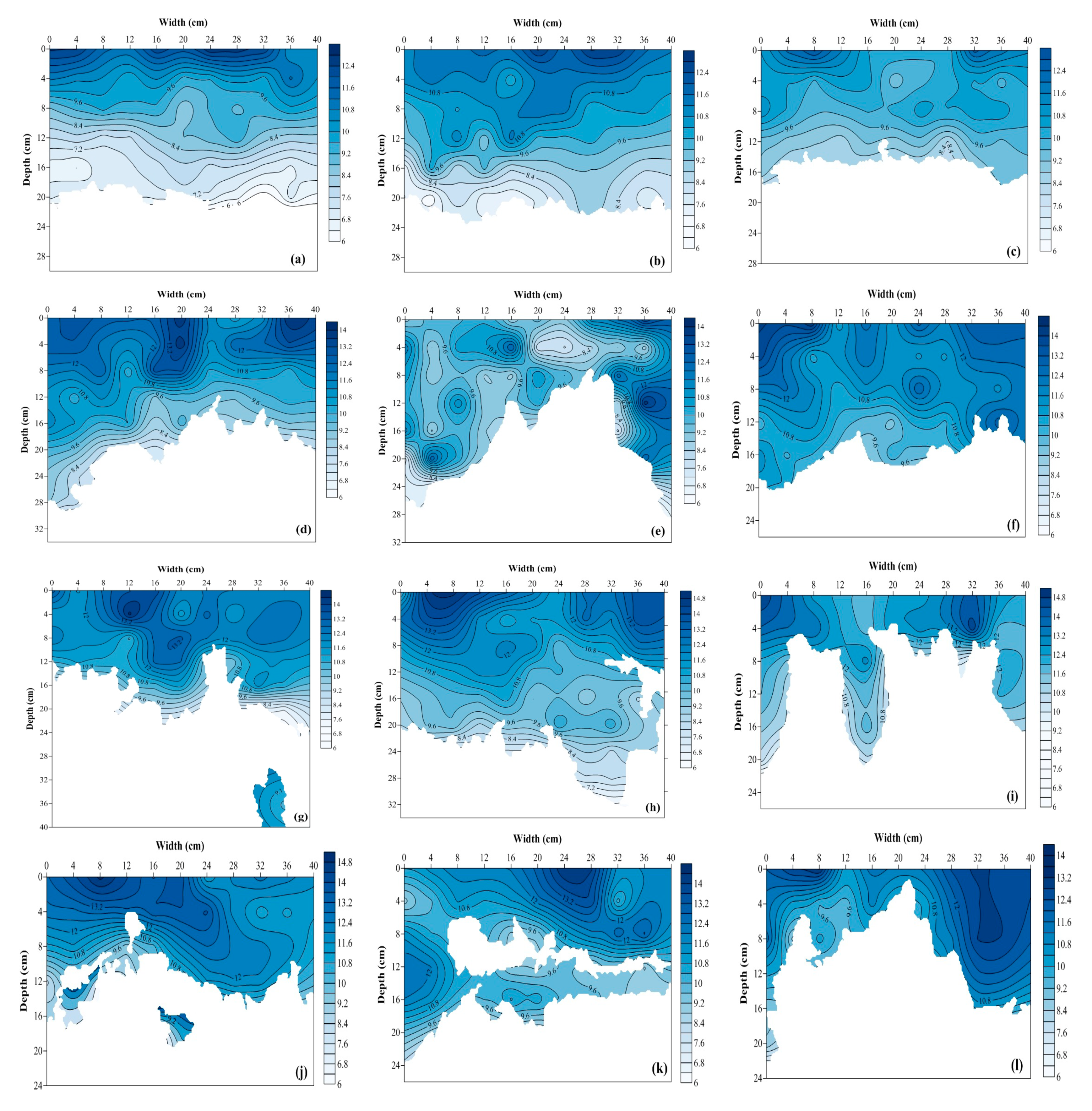
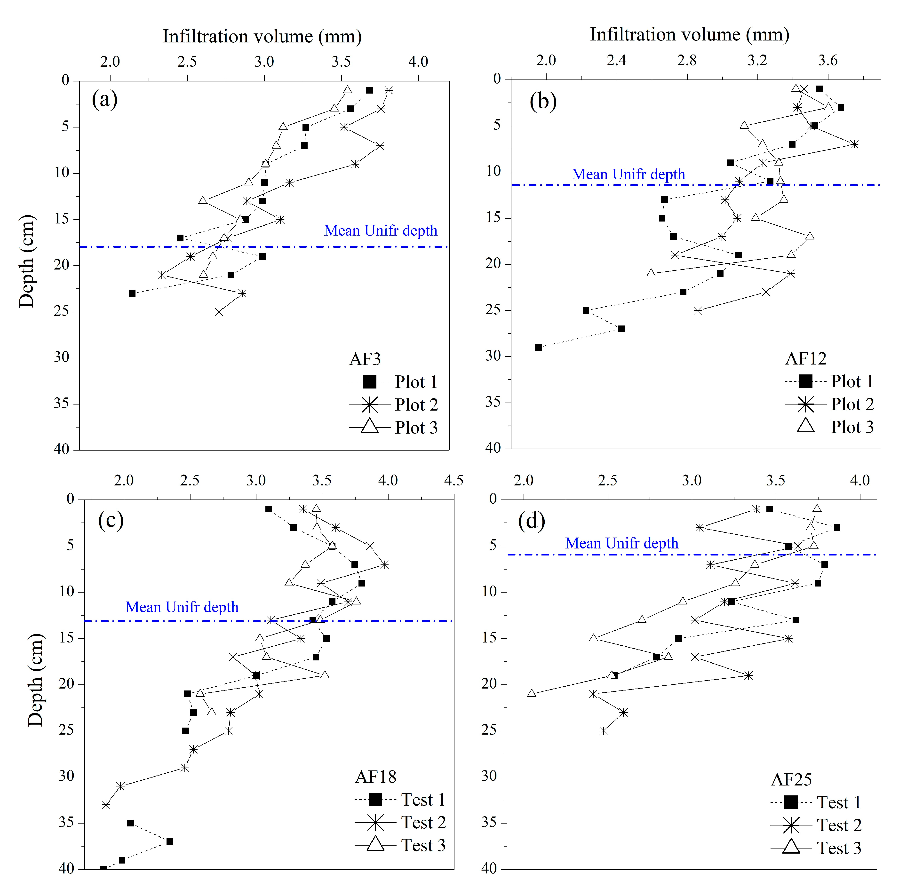
3.2. Infiltration Patterns

The twelve dye stained images of the vertical soil profiles in the four sites are shown in Figure 4. For all images, the non-uniform spreading of the stained region and the uneven wetting front implied that water flowed into the soil along the vertical direction through the preferential pathways and bypassed parts of the soil matrix. However, the stained dye patterns differed in detail among the four sites. In the four sites, the stained region was more evenly distributed, and the wetting front was more stable in AF3 (first row in Figure 4).
With the natural restoration ages, a less uniform distribution of the stained region and a sharper wetting front were observed at AF12 (second row in Figure 4), AF18 (third row in Figure 4) and AF25 (fourth row in Figure 4). Interestingly, parts of the stained region were distributed separately at AF18 (Figure 4g,i), and AF25 (Figure 4j,k), which indicated the infiltration of water into the soil in the two sites also followed other pathways from other directions.
The measured infiltration time and the preferential flow characteristics based on the dye stained images are shown in Table 3. For infiltration time with the same volume of water (62.5 mm), it took about 23.65 min and 24.63 min to infiltrate in AF25 and AF12, respectively, which was significantly less than the time required for AF3 and AF18 to infiltrate, which was about 30.31 min and 38.01 min, respectively. Although the maximum infiltration depth (MID) was 18.00 cm at plot 1 in site AF25 and 32.8 cm at plot 2 in site AF18, the difference of the mean MID was not significant among the four sites.
The least DC was observed in the site AF25, whereas the largest one was observed in AF3. Meanwhile, the longest mean Unifr was found in AF3, indicating the water flowed uniformly through the soil matrix down to the deep depths in this site. However, the FFP, LI, PIV and Con exhibited increasing trends with increasing natural restoration ages. The mean FFP, PIV, LI and Con of the site AF25 was 7.34 times, 4.09 times, 1.17 times and 3.75 times greater than that of the site AF3.

3.3. Contribution of Preferential Flow

Figure 5 shows the vertical distribution of the difference value of SWC before and after irrigation among the four sites with different abandonment time and vegetation communities. With increasing soil depth, the SWC generally decreased for all plots in the four sites. However, the distribution pattern of the SWC was various due to the different water flow pathways network in every soil profile. The higher SWC appeared as the vertical belt was in the contour map, serving as the preferential flow. The belts occurred in the shallow layer of 0–8 cm in site AF3, and in the deep soil layer of about 0–16 cm in AF12, AF18 and AF25. The vertical distribution of the water infiltration volume induced by the dye-stained experiment is shown in Figure 6. The data shows that some water infiltration volume remained mostly below the Unifr depth than above. Besides, compared to AF3, the preferential infiltration volume in AF12, AF18 and AF25 increased by 1.73 times, 1.94 times and 4.09 times, respectively (Table 3).
Table 4 further reveals the spatial distribution of the SWC by the parameters of the semivariogram analysis. For each plot, the best-fit model was performed as it exhibited the greatest R2 and the lowest RSS. The small nugget variances (C0) were observed in all the sites, suggesting that the random variations in the SWC were relatively small. The nugget percentage (C0/(C + C0)) values among the 12 plots were less than 25%, which indicates that the SWC of all the sites exhibited strong spatial dependence. The sill (C0 + C) values and the mean spatial autocorrelation range (A) values increased from AF3 (2.24 and 25.63 cm, respectively) to AF25 (3.49 and 41.88 cm, respectively), and the C0/(C + C0) values decreased from AF3 (6.54) to AF25 (1.51). This suggested that the SWC was more variable as the abandonment time increased.

4. Discussion

4.1. Relationship between the Preferential Water Flow and the Soil and Root Features

The preferential flow occurs in most soils due to the presence of macropores [17], which is closely related to the soil physical properties. Based on the dye tracer experiment, the calculated parameters such as the FFP, PIV and Con (Table 3) could be adopted to estimate the degree of preferential flow. Generally, relatively loose, fragmented and macropore-rich soil were prone to preferential flow [23]. The results of the correlation analysis (Table 5) showed that BD, WR0.25 and SOM had significantly positive relationships with the degree of preferential flow, indicating that lower BD, higher WR0.25 and SOM could enhance the preferential water flow. In general, the reduction of BD was associated with increasing soil porosity [28,29]. Along with decreasing BD, larger aggregates are associated with larger, more widely spaced and more continuous fissures [30]. Kaarakka et al. [31] suggested that SOM decreased the soil BD and increased the soil porosity, thereby inducing to an enhanced infiltration capacity. Hardie et al. reported that high initial SWC could limit the preferential flow [32], but the conclusion derived by Mei et al. [24] was rather the opposite. However, the results provided herein evidenced that the initial SWC had a weak relationship with the preferential flow parameters. Moreover, although Zhang et al.) found that preferential flow was likely to occur in sandy soil [17], soil texture exhibited weak relationship with the preferential flow in our study. The differences was probably ascribed to the different vegetation communities. In their study, the sites were covered by forest, shrub and grass, whereas the abandoned farmland covered by grass or subshrub were selected as our test sites.
Compared with the soil properties, the plant roots and their morphometric features tended to play more important roles on the preferential flow (Table 5), which is in agreement with Perillo et al. [33], who found that both decaying and living root systems were the most pivotal agents for preferential flow pathways. Cui et al. also found that fine roots were the main factor affecting the potential of soil infiltration in semi-arid regions [34]. During plant root growth, the plant roots not only grow into the preferential flow pathway, but they also create the pathways through biopores, cracks and burrows [17]. On the other hand, growing root systems were associated with reducing soil BD and increasing WR0.25 and SOM in our study (Table 2 and Figure 3). This finding is supported by Benegas et al. [12], who found that the inputs of plant root were critical for improving soil properties during vegetation recovery, thereby motivating preferential flow. In the present study, all the four root features showed positive correlations with the content of the preferential flow. The distribution of the dye stained area corresponded to the distribution regions of the root system (Figure 3), and the preferential flow ended at the layers with fewer roots. The values of RMD, RVD, RD and RLD were the greatest in AF25 in comparison with AF3. Hence, the preferential flow was substantially stronger in AF25 than in AF3, which is consistent with the results reported by Zhang et al. [35], who found that RMD and RLD were greater in preferential pathways than in the soil matrix. Huang et al. [36] also revealed that RMD was the most important factor for the infiltration process. However, Cui et al. [34] found that non-perishable coarse roots could compact soil and block water flow, thereby causing more RMD inhibited soil infiltration process. The differences may be attributed to the variations in the root morphology and the root distribution in the soil profiles amongst the different plant species [22].

4.2. Variation Patterns of Water Flow Behaviors during Natural Vegetation Restoration

In the abandoned farmlands without ploughing and sowing, the soil physicochemical properties and the below-ground biomass changed greatly with vegetation restoration [3]. In the present study, as the abandonment time increased, vegetation restoration not only improved the soil and root properties (Table 2 and Figure 3), but also had different effects on water flow behaviors, as illustrated by the visual dye tracer information (Figure 4) and the preferential flow parameters (Table 3). Although the soil matrix flow was initiated near the soil surface, the preferential flow became the dominant flow behavior after years of abandonment. The degree of preferential flow from lowest to highest occurred in AF3, AF12, AF18 and AF25 (Table 3), following the increasing natural restoration ages. These results confirmed the vital effect of root systems on the formation of preferential flow pathways. Plant root mass density greatly increased with vegetation restoration age both at hillslopes and steep gully slopes in the Loess Plateau [4], which agreed with the present results (Figure 3). The AF3 site, which was dominated by the short-lived grass of Artemisia scoparia with small amount roots, had the lowest extent of preferential flow, suggesting that a significant portion of infiltrating water flowed uniformly through the soil matrix. This finding is in agreement with the conclusion of Jiang [13], who found that the matrix flow was the dominant flow type in the soil profile with no roots. Compared to the site AF3, the dominant vegetation in AF12, AF18 and AF25 were respectively the perennial grass, the subshrub and the shrub with more abundant and dense root systems, resulting in a greater preferential flow. Similarly, Alaoui et al. found that forestlands exhibited greater preferential flow than grasslands [10]. Moreover, old root channels and some wormholes were also found through the soil profile in the field (Figure 4e,h,i,l)), which could form numerous continuous macropores and preferential paths [37]. Old or decaying roots and animal activates are believed to increase with natural restoration ages.
Water flow bypassed the soil matrix and confined it to isolate patches, thereby exhibiting typical flow behavior in AF18 and AF25, which was known as lateral flow (Figure 4g,i,j,k)). In agreement with Sheng et al. [38], the lateral flow was found to be not obvious in the upper soil layers (<10 cm), while it may have been more predominate with increasing soil depth. Jiang et al. revealed that lateral flow occurred when a wetting front penetrated through the soil layers [23]. The factors that influence lateral flow include the soil matrix properties, the macropores, and the macropore-matrix interface [13]. The Bothriochloa ischaemum that dominated in AF18 possessed abundant fine roots and intricate fibrous roots. The channels of random directions created by the dense root network contributed to the non-uniform water movement and the irregular wetting front, likely causing the phenomenon of lateral flow. The Periploca sepium bunge in AF25, which had developed taproot and lateral root, offered potential lateral directions for water infiltration. Also, the relatively steeper slope may further promote the phenomena of lateral flow [39]. In the present study, Figure 4g shows that the isolated patches that occurred at the bottom of the soil profile was far from the upper macrospore flow in Plot 1 in site AF18 with slope gradient of 20°, which may be attributed the lateral water movement from the upper slope driven by gravity from the upper slope. This finding was distressed from those obtained by Jiang et al. [23], who found that compacted matrix by tillage pan and high SWC in cropland lead to the emergence of lateral flow.

4.3. Contribution of the Preferential Flow on Soil Water Storage

Spatial distribution maps of the soil water content better represented the water infiltration process and the preferential flow pathways than the dye-stain images [24]. As shown in Figure 5, the belt with high moisture content was associated with macropore flow paths. The depths of those belts were prone to be deeper as the degree of preferential flow was greater with increasing abandonment time. This result is consistent with the finding reported by Malvar et al. who found that water may concentrate in macrospores and cause preferential flow paths, thereby leaving the surrounding soil matrix relatively dry [40]. Further, it is worth noting that the infiltration volume below Unfir tended to increase with increasing soil depth (Figure 6), which therefore demonstrates that the preferential pathways in the soil profile could promote the delivery of water flow into the deep soil layer. This result agreed with Hanson et al. who reported that preferential flow paths and large macrospores carried most of the water when the soil became saturated [41]. Previous studies indicated that several scattered areas with high water infiltration might be caused by the rock fragment of soil in forests [42] and tillage practice in croplands [23]. However, this phenomenon was herein related to the lateral flow, which was probably induced by the non-uniform void of the soil created by the plant roots and worm holes.
Based on semivariograms analysis, the nugget percentage values of C0/(C + C0) were less than 25% in all sites, indicating that the water flow pattern had strong spatial dependence among the four sites with different natural restoration time. Moreover, the spatial heterogeneity of the SWC increased from AF3 to AF25 with the increasing abandonment time. The stronger spatial heterogeneity of the SWC may be induced by the greater degree of preferential flow with the non-uniform soil properties and root systems [43]. Therefore, the improved preferential flow led to the vertical and lateral redistribution of the soil water, and increased water storage in the soil profile, which was in favor of the plant growth and sustainability of vegetation restoration.
Additionally, dye tracer images do not quantify soil macopores and 3-D soil macropore networks, although it can visually reveal the vertical water flow patterns and preferential flow pathways. Future research should prefer to the methods of X-ray computed tomography (CT) and dye tracer along the different direction.

5. Conclusions

This study quantified the temporal variations in water flow behaviour of different vegetation communities in abandoned farmlands on the Loess Plateau. The results showed that the soil organic matter content (SOM) and the water stable aggregate (>0.25 mm) content (WR0.25) increased with natural restoration age, while the bulk density (BD) decreased from AF3 to AF25. The natural restoration age combined with the plant species induced a positive effect on the root mass density (RMD), the root volume density (RVD), the root diameter (RD) and the root length density (RLD). These improved soil properties and developed root systems substantially influenced the water flow behavior and enhanced the degree of preferential flow.
The results of the dye tracer experiment and the image analysis indicated that the mean FFP, PIV, LI and Con of AF25 were 7.34 times, 4.09 times, 1.17 times and 3.75 times greater than that of AF3. The correlation analysis implied that the plant roots and their morphometric features exhibited a greater effect on the preferential flow in comparison with the soil properties. The abundant lateral root and the steeper slope may have caused the presence of lateral flow that occurred in AF18 and AF25.
Moreover, the contour map of the soil water content showed a belt of high soil water content spread into the deeper soil layer with longer restoration ages. The spatial variability of the soil water through the vertical soil profiles increased from AF3 to AF25 with increasing degree of preferential flow. Also, the contribution of the preferential flow to the total infiltration increased with abandonment time. Therefore, the improvement of the preferential flow in the abandoned farmland during natural vegetation restoration helped soil water storage in the deep soil layer.

Author Contributions

R.W. processed the datasets, implemented the methodology, and finished the manuscript. Z.D. guided the results and discussion. Z.Z. contributed to reviewing and editing. P.W. contributed to data presentation.

Funding

The research was funded by National Natural Science Foundation of China (41807061, 41930641, 41977061), Postdoctoral Science Foundation of China (2018M633454), Fundamental Research Funds for the Central Universities of China (GK201803046), and National Key Research and Development Plan of China (2017YFC0504702).

Acknowledgments

The authors would like to thank the reviewers and the editor whose suggestions greatly improved the manuscript.

Conflicts of Interest

The authors declare no conflict of interest.

References

  1. Zhang, G.H.; Tang, M.K.; Zhang, X.C. Temporal variation in soil detachment under different land uses in the Loess Plateau of China. Earth Surf. Process. Landf. 2010, 34, 1302–1309. [Google Scholar] [CrossRef]
  2. An, S.S.; Darboux, F.; Cheng, M. Revegetation as an efficient means of increasing soil aggregate stability on the Loess Plateau (China). Geoderma 2013, 209, 75–85. [Google Scholar] [CrossRef]
  3. Hou, J.; Fu, B.J.; Liu, Y.; Lu, N.; Gao, G.Y.; Zhou, J. Ecological and hydrological response of farmlands abandoned for different lengths of time: Evidence from the Loess Hill Slope of China. Glob. Planet. Chang. 2014, 113, 59–67. [Google Scholar] [CrossRef]
  4. Zhang, B.J.; Zhang, G.H.; Yang, H.Y.; Zhu, P.Z. Temporal variation in soil erosion resistance of steep slopes restored with different vegetation communities on the Chinese Loess Plateau. Catena 2019, 182, 104–170. [Google Scholar] [CrossRef]
  5. Tang, B.Z.; Jiao, J.Y.; Yan, F.C.; Li, H. Variations in soil infiltration capacity after vegetation restoration in the hilly and gully regions of the Loess Plateau, China. J. Soils Sediments 2019, 19, 1456–1466. [Google Scholar] [CrossRef]
  6. Jiao, J.Y.; Tzanopoulos, J.; Xofis, P.; Mitchley, J. Factors affecting distribution of vegetation types on abandoned cropland in the hilly-gullied Loess Plateau region of China. Pedosphere 2008, 18, 24–33. [Google Scholar] [CrossRef]
  7. Yu, Y.; Wei, W.; Chen, L.D.; Feng, T.J.; Daryanto, S.; Wang, L.X. Land preparation and vegetation type jointly determine soil conditions after long-term land stabilization measures in a typical hilly catchment, Loess Plateau of China. J. Soils Sediments 2017, 17, 144–156. [Google Scholar] [CrossRef]
  8. Cerdà, A. Seasonal variability of infiltration rates under contrasting slope conditions in southeast Spain. Geoderma 1996, 69, 217–232. [Google Scholar] [CrossRef] [Green Version]
  9. Stumpp, C.; Maloszewski, P. Quantification of preferential flow and flow heterogeneities in an unsaturated soil planted with different crops using the environmental isotope δ18O. J. Hydrol. 2010, 394, 407–415. [Google Scholar] [CrossRef]
  10. Alaoui, A.; Caduff, U.; Gerke, H.H.; Weingartner, R. A preferential flow effects on infiltration and runoff in grassland and forest soils. Vadose Zone J. 2011, 10, 367–377. [Google Scholar] [CrossRef]
  11. Allaire, S.E.; Roulier, S.; Cessna, A.J. Quantifying preferential flow in soils: A review of different techniques. J. Hydrol. 2009, 378, 179–204. [Google Scholar] [CrossRef]
  12. Bargués, T.A.; Reese, H.; Almaw, A.; Bayala, J.; Malmer, A.; Laudon, H.; Ilstedt, U. The effect of trees on preferential flow and soil infiltrability in an agroforestry parkland in semiarid Burkina Faso. Water Resour. Res. 2014, 50, 3342–3354. [Google Scholar] [CrossRef] [Green Version]
  13. Jiang, X.J.; Liu, W.; Chen, C.; Liu, J.; Yuan, Z.Q.; Jin, B.; Yu, X. Effects of three morphometric features of roots on soil water flow behavior in three sites in China. Geoderma 2018, 320, 161–171. [Google Scholar] [CrossRef]
  14. Holman, I.P.; Dubus, I.G.; Hollis, J.M.; Brown, C.D. Using a linked soil model emulator and unsaturated zone leaching model to account for preferential flow when assessing the spatially distributed risk of pesticide leaching to groundwater in England and Wales. Sci. Total. Environ. 2004, 318, 73–88. [Google Scholar] [CrossRef] [Green Version]
  15. Flury, M.; Flühler, H. Brilliant Blue FCF as a dye tracer for solute transport studies—A toxicological overview. J. Environ. Qual. 1994, 23, 1108–1112. [Google Scholar] [CrossRef]
  16. Van Schaik, N. Spatial variability of infiltration patterns related to site characteristics in a semi-arid watershed. Catena 2009, 78, 36–47. [Google Scholar] [CrossRef]
  17. Zhang, Y.; Niu, J.; Zhang, M. Interaction between plant roots and soil water flow in response to preferential flow paths in northern China. Land Degrad. Dev. 2017, 28, 648–663. [Google Scholar] [CrossRef]
  18. Beven, K.; Germann, P. Macropores and water flow in soils revisited. Water Resour. Res. 2013, 49, 3071–3092. [Google Scholar] [CrossRef] [Green Version]
  19. Truax, B.; Gagnon, D.; Fortier, J.; Lambert, F. Yield in 8 year-old hybrid poplar plantations on abandoned farmland along climatic and soil fertility gradients. For. Ecol. Manag. 2012, 267, 228–239. [Google Scholar] [CrossRef]
  20. Wang, H.; Zhang, G.H.; Li, N.N.; Zhang, B.J.; Yang, H.Y. Variation in soil erodibility under five typical land uses in a small watershed on the Loess Plateau, China. Catena 2019, 174, 24–35. [Google Scholar] [CrossRef]
  21. Raiesi, F. Land abandonment effect on N mineralization and microbial biomass N in a semi-arid calcareous soil from Iran. J. Arid Environ. 2012, 76, 80–87. [Google Scholar] [CrossRef]
  22. Ola, A.; Dodd, I.C.; Quinton, J.N. Can we manipulate root system architecture to control soil erosion? Soil 2015, 1, 603–612. [Google Scholar] [CrossRef] [Green Version]
  23. Jiang, X.; Liu, X.; Wang, E. Effects of tillage pan on soil water distribution in alfalfa-corn crop rotation systems using a dye tracer and geostatistical methods. Soil Tillage Res. 2015, 150, 68–77. [Google Scholar] [CrossRef]
  24. Mei, X.; Zhu, Q.; Ma, L. Effect of stand origin and slope position on infiltration pattern and preferential flow on a Loess hillslope. Land Degrad. Dev. 2018, 29, 1353–1365. [Google Scholar] [CrossRef]
  25. Cey, E.E.; Rudolph, D.L. Field study of macropore flow processes using tension infiltration of a dye tracer in partially saturated soils. Hydrol. Process. 2009, 23, 1768–1779. [Google Scholar] [CrossRef]
  26. Yu, Y.; Loiskandl, W.; Kaul, H.P.; Himmelbauer, M.; Wei, W.; Chen, L.D.; Bodner, G. Estimation of runoff mitigation by morphologically different cover crop root system. J. Hydrol. 2016, 538, 667–676. [Google Scholar] [CrossRef] [Green Version]
  27. Burgos, P.; Engracia, M.; Alfredo, P. Spatial variability of the chemical characteristics of a trace-element-contaminated soil before and after remediation. Geoderma 2006, 130, 157–175. [Google Scholar] [CrossRef]
  28. Yu, Y.; Wei, W.; Chen, L.D.; Feng, T.J.; Daryanto, S. Quantifying the effects of precipitation, vegetation, and land preparation techniques on runoff and soil erosion in a Loess watershed of China. Sci. Total. Environ. 2019, 652, 755–764. [Google Scholar] [CrossRef]
  29. Singh, Y.P.; Nayak, A.K.; Sharma, D.K.; Singh, G.; Mishra, V.K.; Singh, D. Evaluation of Jatropha curcas genotypes for rehabilitation of degraded sodic lands. Land Degrad. Dev. 2015, 26, 510–520. [Google Scholar] [CrossRef]
  30. Jarvis, N.J. A review of non-equilibrium water flow and solute transport in soil macropores: Principles, controlling factors and consequences for water quality. Eur. J. Soil Sci. 2007, 58, 523–546. [Google Scholar] [CrossRef]
  31. Kaarakka, L.; Smolander, A.; Lindroos, A.J.; Nojd, P.; Korpela, L.; Nieminen, T.M.; Helmisaari, H.S. Sprinkling infiltration as an artificial groundwater recharge method—Long-term effects on boreal forest soil, tree growth and understory vegetation. For. Ecol. Manag. 2019, 448, 240–248. [Google Scholar] [CrossRef]
  32. Hardie, M.A.; Cotching, W.E.; Doyle, R.B.; Holz, G.; Lisson, S.; Mattern, K. Effect of antecedent soil moisture on preferential flow in a texture-contrast soil. J. Hydrol. 2011, 398, 191–201. [Google Scholar] [CrossRef]
  33. Perillo, C.A.; Gupta, S.C.; Nater, E. Prevalence and initiation of preferential flow paths in a sandy loam with argillic horizon. Geoderma 1999, 89, 307–331. [Google Scholar] [CrossRef]
  34. Cui, Z.; Wu, G.L.; Huang, Z.; Liu, Y. Fine roots determine soil infiltration potential than soil water content in semi-arid grassland soils. J. Hydrol. 2019, 578, 124023. [Google Scholar] [CrossRef]
  35. Zhang, Y.; Niu, J.; Yu, X.; Zhu, W.; Du, X. Effects of fine root length density and root biomass on soil preferential flow in forest ecosystems. For. Syst. 2015, 24, 12. [Google Scholar] [CrossRef] [Green Version]
  36. Bodner, G.; Loiskandl, W.; Buchan, G.; Kaul, H.P. Natural and management-induced dynamics of hydraulic conductivity along a cover-cropped field slope. Geoderma 2008, 146, 317–325. [Google Scholar] [CrossRef]
  37. Hamilton, G.J.; Bakker, D.; Akbar, G.; Hassan, I.; Hussain, Z.; McHugh, A.; Raine, S. Deep blade loosening increases root growth, organic carbon, aeration, drainage, lateral infiltration and productivity. Geoderma 2019, 345, 72–92. [Google Scholar] [CrossRef]
  38. Sheng, F.; Wang, K.; Zhang, R.D. Study on heterogeneous characteristics of soil water flow in field by dye tracing method. J. Hydraul. Eng. 2009, 40, 101–108. [Google Scholar]
  39. Klos, P.Z.; Chain-Guadarrama, A.; Link, T.E.; Finegan, B.; Vierling, L.A.; Chazdon, R. Throughfall heterogeneity in tropical forested landscapes as a focal mechanism for deep percolation. J. Hydrol. 2014, 519, 2180–2188. [Google Scholar] [CrossRef]
  40. Malvar, M.C.; Prats, S.A.; Nunes, J.P.; Keizer, J.J. Soil water repellency severity and its spatio-temporal variation in burnt eucalypt plantations in North-Central Portugal. Land Degrad. Dev. 2016, 27, 1463–1478. [Google Scholar] [CrossRef]
  41. Hanson, D.L.; Steenhuis, T.S.; Walter, M.F.; Boll, J. Effects of soil degradation and management practices on the surface water dynamics in the Talgua River watershed in Honduras. Land Degrad. Dev. 2004, 15, 367–381. [Google Scholar] [CrossRef]
  42. Sohrt, J.; Ries, F.; Sauter, M. Significance of preferential flow at the rock soil interface in a semi-arid karst environment. Catena 2014, 123, 1–10. [Google Scholar] [CrossRef]
  43. Shinohara, Y.; Otsuki, K. Comparisons of soil-water content between a Moso bamboo (Phyllostachys pubescens) forest and an evergreen broadleaved forest in western Japan. Plant Species Biol. 2015, 30, 96–103. [Google Scholar] [CrossRef]
Figure 1. Location of the study area and experimental sites. AF means the abandoned farmland and the number means the abandonment time.
Land 08 00186 g001
Figure 2. Example of image processing at Plot 3 in site AF18, and the raw image (a), the black and white binary image (b), and parameter extractions (c).
Land 08 00186 g002
Figure 3. Root mass density (RMD) (a), root volume density (RVD) (b), root mean diameter (RD) (c) and root length density (RLD) (d) in different soil layers of the four sites. The value represents mean ± SD, n = 3.
Land 08 00186 g003
Figure 4. Stained images for vertical soil profiles in the four sites. (ac) in first row are Plot 1, Plot 2 and Plot 3 in site AF3, respectively; (df) in second row are Plot 1, Plot 2 and Plot 3 in site AF12, respectively; (gi) in third row are Plot 1, Plot 2 and Plot 3 in site AF18, respectively; (jl) in fourth row are Plot 1, Plot 2 and Plot 3 in site AF25, respectively.
Land 08 00186 g004
Figure 5. Spatial maps of distributions of SWC (%) in the vertical soil profiles in the four sites. (ac) in first row are Plot 1, Plot 2 and Plot 3 in site AF3, respectively; (df) in second row are Plot 1, Plot 2 and Plot 3 in site AF12, respectively; (gi) in third row are Plot 1, Plot 2 and Plot 3 in site AF18, respectively; (jl) in fourth row are Plot 1, Plot 2 and Plot 3 in site AF25, respectively.
Land 08 00186 g005
Figure 6. Distribution of soil water infiltration volume along soil profile in site AF3 (a), AF12 (b), AF18 (c) and AF25 (d).
Land 08 00186 g006
Table 1. Elementary information on the experimental sites.
SiteAltitude (m)Slope Aspect (°)Slope Gradient (°)Slope Length(m)Vegetation Coverage (%)Dominant Communities
AF31157NE80114335Artemisia scoparia-Green bristle grass
AF121233NE55185544Artemisia sacrorum-Artemisia argyi
AF181254NE65206637Bothriochloa ischaemum-Artemisia sacrorum
AF251287NE30165847Periploca sepium Bunge-Artemisia sacrorum
Note: AF means the abandoned farmland and the number means the abandonment time.
Table 2. Mean soil properties (0–40 cm soil layer depth) of different sites.
SiteBD (g/cm3)SWC (%)SOM (g/kg)WR0.25 (%)Soil Particle Size Distribution
Clay (%)Silt (%)Sand (%)
AF31.31 ± 0.03 a10.07 ± 0.05 b4.67 ± 0.03 b29.45 ± 1.46 c10.73 ± 0.01 a 23.15 ± 0.23 a66.12 ± 0.73 a
AF121.27 ± 0.01 b 11.02 ± 0.08 a4.60 ± 0.05 b 39.44 ± 1.93 b10.80 ± 0.01 a23.55 ± 0.09 a 65.66 ± 0.16 a
AF181.22 ± 0.01 c9.34 ± 0.06 c4.87 ± 0.05 b46.64 ± 1.62 a11.25 ± 0.01 a 24.62 ± 0.54 a 65.13 ± 0.51 a
AF251.14 ± 0.01 d10.68 ± 0.01 a5.28 ± 0.08 a48.26 ± 2.16 a11.54 ± 0.12 a25.23 ± 1.09 a64.23 ± 1.58 a
Note: Data represent means ± standard deviation (n = 3 replications × 4 soil layers = 12). Different letters in one column represent significant difference at p < 0.05 among different sites.
Table 3. Dye stain characteristics in the vertical soil profiles for the twelve plots of four sites.
SiteITMIDUnifrDCFFPLIPIVCon
(min)(cm)(cm)(%)(%)(mm)(%)
AF3
Plot 129.6023.218.950.446.32273.75 5.0313.85
Plot 232.5024.620.855.285.93327.50 3.9211.46
Plot 329.5019.91435.120.34280.00 6.8226.34
Mean30.31 ± 0.98 a22.57 ± 1.19 a 17.9 ± 3.50 a46.95 ± 10.52 a4.2 ± 3.35 b293.75 ± 16.97 a 5.26 ± 1.46 b17.22 ± 7.99 b
AF12
Plot 120.6029.51543.8614.5436.75 16.1941.58
Plot 229.60248.137.2145.58242.00 17.0653.2
Plot 323.7020.411.437.1523.28226.75 9.7935.59
Mean24.63 ± 2.64 b 24.63 ± 4.58 a11.5 ± 3.54 a39.41 ± 3.86 a27.79 ± 16.02 a301.83 ± 69.14 a 14.35 ± 3.97 a43.45 ± 8.95 a
AF18
Plot 143.2025.91344.2626.57402.00 13.3840.71
Plot 235.5032.821.255.444.4361.50 12.7931.2
Plot 336.60224.523.8852.89185.25 20.2772.21
Mean38.01 ± 2.40 a 26.9 ± 5.46 a12.9 ± 8.35 a41.19 ± 16.00 a27.95 ± 24.27 a316.25 ± 79.41 a 15.48 ± 4.16 a48.04 ± 21.46 a
AF25
Plot 125.7018928.1219.99386.00 9.241.99
Plot 227.6025.35.935.5141.54331.25 30.1672.37
Plot 317.90222.822.6530.91291.75 25.0779.33
Mean23.65 ± 2.96 b 21.77 ± 3.66 a5.9 ± 3.10 c28.76 ± 6.45 a30.81 ± 10.78 a336.33 ± 27.32 a 21.48 ± 10.93 a64.56 ± 19.85 a
Note: IT means the infiltration time, MID means the maximum infiltration depth, Unifr means the uniform infiltration depth, DC means the dye coverage to the total soil profile region, FFP means the preferential flow proportion, LI means the length index, PIV means the preferential infiltration volume, Con means the contribution of the preferential infiltration to the total infiltration. The mean value of each site represents mean ± SD, n = 3. The different letters for mean value in one column represent a significant difference at p < 0.05 among different sites.
Table 4. Geostatistical analysis of the main characteristics of the SWC in the four sites.
SiteModelNugget (C0)Sill (C0 + C)A(cm)C0/(C + C0) (%)R2RSS
AF3
Plot 1Sp0.04042.6027.221.550.8940.0019
Plot 2Ga0.45263.5628.8312.710.9990.0011
Plot 3Sp0.03050.5720.855.360.9340.0017
Mean 0.1745 ± 0.1460 a2.24 ± 1.23 b25.63 ± 4.22 b6.54 ± 2.39 a0.9430.0016
AF12
Test 1Ex0.15453.6442.214.250.9340.0010
Test 2Ex0.15771.5219.8110.360.8650.0021
Test 3Ex0.06512.2754.572.870.8910.0016
Mean 0.1258 ± 0.0303 a2.48 ± 1.07 b38.86 ± 9.70 a5.82 ± 2.30 a0.8970.0016
AF18
Test 1Ex0.05853.6549.571.600.9140.0013
Test 2Ex0.04634.7646.370.970.9240.0011
Test 3Ex0.06461.2426.625.230.8540.0023
Mean 0.0565 ± 0.0054 b3.22 ± 1.04 a40.85 ± 7.98 a2.60 ± 1.32 b0.8970.0016
AF25
Test1Ex0.00645.4256.570.120.9030.0016
Test 2Sp0.00741.9336.930.380.9100.0016
Test 3Ga0.12603.1332.134.030.8640.0056
Mean 0.0466 ± 0.0039 b3.49 ± 1.02 a41.88 ± 11.65 a1.51 ± 1.26 b0.8920.0029
Note: Sp means the spherical model; Ga means the Gaussian model; Ex means the exponential model; RSS means the residual sum of squares. The mean value of each site represents mean ± SD, n = 3. The mean value of each site represents mean ± SD, n = 3. The different letters for mean value in one column represent significant difference at p < 0.05 among different sites.
Table 5. Person coefficients between preferential water flow parameters and soil and plant root characteristics.
ItemsSoil Root
BDSWCSOMWR0.25ClaySiltSandRMDRVDRDRLD
IT 0.3570.527−0.401−0.085−0.308−0.2120.112−0.358−0.597 *−0.493−0.416
MID0.199−0.176−0.332−0.565 *0.2680.253−0.2370.542 *0.804 **0.613 *−0.503 *
Unifr0.707 **−0.059−0.638 *−0.7210.2670.396−0.306−0.738 **−0.780 **−0.290−0.674 **
DC0.306−0.108−0.342−0.424−0.3770.2980.239−0.342−0.155−0.485−0.341
FFP−0.715 **0.0820.652 **0.686 **0.1510.236−0.1780.873 **0.805 **0.537 *0.612 *
LI−0.601 *−0.0830.562 *0.726 **0.2130.144−0.2580.783 **0.648 *0.572 *0.589 *
PIV−0.713 **−0.0760.573 *0.621 *0.1520.294−0.2140.818 **0.733 **0.659 **0.711 **
Con−0.675 **−0.0780.5370.656 *0.1550.286−0.1920.778 **0.735 **0.607 *0.728 **
Note: ** means the significant correlation at 0.01 level (p < 0.01); * means the significant correlation at 0.05 level (p < 0.05).

