Experiences from a National Landscape Monitoring Programme—Maintaining Continuity Whilst Meeting Changing Demands and Opportunities


NIBIO Norwegian Institute of Bioeconomy Research, Department of Landscape Monitoring, NO-1431 Ås, Norway
*
Author to whom correspondence should be addressed.
Land 2019, 8(5), 77; https://0-doi-org.brum.beds.ac.uk/10.3390/land8050077
Submission received: 11 March 2019
/
Revised: 11 April 2019
/
Accepted: 26 April 2019
/
Published: 30 April 2019
(This article belongs to the Special Issue European Landscapes and Quality of Life)
Abstract
:Over the past few decades, there has been increasing interest in recording landscape change. Monitoring programmes have been established to measure the scope, direction and rate of change, and assess the consequences of changes for multiple interests, such as biodiversity, cultural heritage and recreation. The results can provide feedback for multiple sectors and policy domains. Political interests may change over time, but long-term monitoring demands long-term funding. This requires that monitoring programmes remain relevant and cost-efficient. In this paper, we document experiences from 20 years of the Norwegian Monitoring Programme for Agricultural Landscapes—the ‘3Q Programme’. We explain how data availability and demands for information have changed over time, and how the monitoring programme has been adapted to remain relevant. We also discuss how methods of presentation influence the degree of knowledge transfer to stakeholders, in particular to policy makers.
1. Introduction
Landscapes are forever changing, with wide-ranging consequences for both people and wildlife. To gain an overview over these changes, and enable action to avoid negative consequences, there has been increasing recognition of the need for monitoring [1,2,3]. Many countries have established monitoring programmes, for example the British Countryside Survey [4], the Northern Ireland Countryside Survey [5], the Swiss Landscape Monitoring Programme [6] and the Swiss Monitoring of Agricultural Species and Habitats [7], the National Inventory of Landscapes in Sweden [8], and the High Nature Value Farmland Monitoring in Germany [9]. Nevertheless, information about national monitoring programmes is rare in the international scientific literature, and national level grey literature often targets a different kind of audience and does not include information about the methodological challenges and technical details that might be useful for those who are running monitoring programmes themselves with some exceptions, e.g., [10]. In this paper, we present our experiences from 20 years of monitoring and discuss methodological dilemmas and challenges of communicating monitoring results. Our aim is to share experiences and considerations that may be relevant for others working with landscape monitoring, both those responsible for designing and running monitoring programmes, and those using the results from such programmes.
The Norwegian monitoring programme for agricultural landscapes (“the 3Q Programme”) started in 1998, financed jointly by the Norwegian Ministry of Agriculture and Ministry of the Environment. The main objective was to document status and change in agricultural landscapes, as a basis from which to evaluate the effectiveness of agricultural and environmental policies and contribute to their improvement [11]. Four themes of interest were defined: (i) The spatial structure of the landscape, (ii) biodiversity, (iii) cultural heritage, and (iv) accessibility. For cost-effectiveness, the 3Q Programme was to be based on interpretation of aerial photographs, using indicators to express change for the four topics. The indicators were to be based primarily on map data, i.e., land types, land use intensity (as far as can be deduced from aerial photographs), and the amounts and spatial arrangement of various landscape elements. Statistical sampling was designed to indicate development trends at national and regional levels.
A fundamental aspect of monitoring is that results should be comparable over time [12]. Ideally this involves strict adherence to the same methodology with each round of recording. Nevertheless, for several reasons, there have been changes in the methods used in the 3Q Programme. Firstly, the programme is under constant pressure to be cost-efficient, and this entails using new technologies and new data sources wherever possible to reduce costs. Secondly, demands for information have changed over the years. For example, there is now interest in monitoring a wider range of landscape types than were planned for when the programme was initiated. The programme must also be somewhat flexible in order to survive variations in interest from authorities and therefore budgets over time. In the following sections, we describe the changes that have been made, the reasons for each change, the consequences in terms of the results that can be reported and the certainty of estimates. We discuss how opportunities and demands from the programme have changed over time and how the methodology has changed to maintain relevance for policy makers.
2. Methods
2.1. Original 3Q Methods
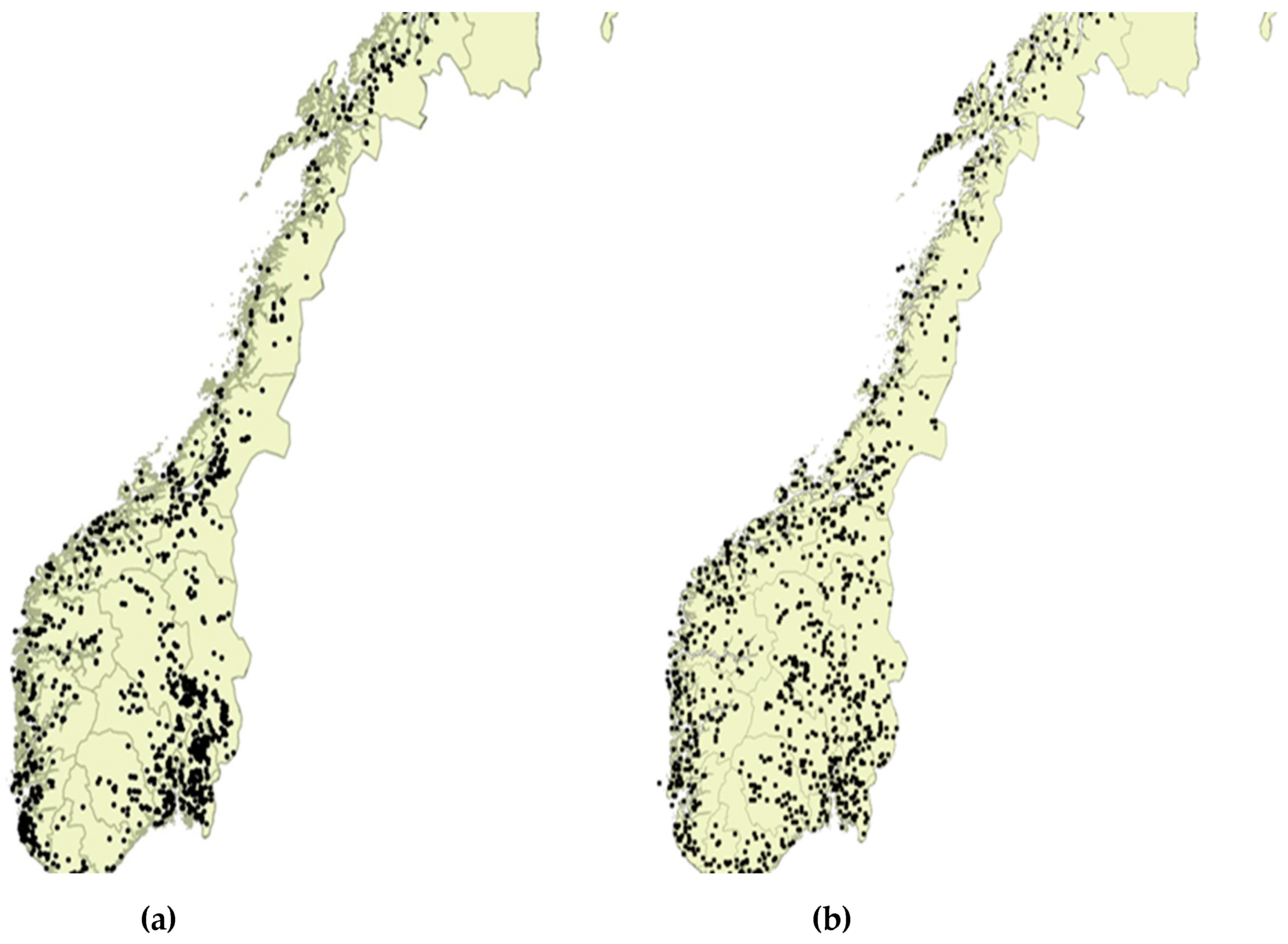
The 3Q Programme was originally based on aerial photography of a systematic stratified sample of 1474 monitoring squares of 1 × 1 km (Figure 1). These sample squares were located using the 3 × 3 km grid already established for sampling in the national forest inventory (NFI) of Norway [13]. Where a grid point fell on forest land types, an NFI sample point was established. If the point fell on land used for agricultural purposes (as defined by the Economic Map Series), a 1 × 1 km square centred on this point was included in the 3Q monitoring sample. Stratification of the sample to agricultural land was necessary because agriculture is an uncommon land type in Norway, comprising only 3% of the land area in total and scattered throughout the entire country. Agriculture would therefore be poorly represented in a random sample. This stratified sampling method resulted in monitoring squares distributed across the country in proportion to the amount of agricultural land (Figure 1). In practice, the budget was never sufficient to analyse all 1474 squares and a random sample of 70% was selected as “first priority”.
Land types within each square were digitized according to a hierarchical classification system, with approximately 100 land types at the most detailed level [11] (Table 1). In addition, linear elements (less than 2 m wide) and point objects (larger than 4 m2, but smaller than 100 m2) were recorded, including both natural and cultural features. The minimum size for digitizing polygons belonging to the class ‘agricultural land’, or having a joint border with an area belonging to that class, was 100 m2. For other areas the minimum size was 1000 m2, reflecting the focus on agricultural areas in the 3Q Programme. A wide array of landscape metrics was calculated based on the digitized maps, and these formed the basis for reported indicators [11] (see examples in Table 2).
The monitoring was conducted according to a five-year inventory cycle, with approximately 20% of the sample squares being photographed and mapped each year. The first national set of aerial photographs was planned to be completed in 2002 but was achieved in 2003. For the second national set, most photographs were available by 2007, but full coverage was reached two years later.
In order to estimate county statistics from the sample squares, a scaling factor was used for each county. The scaling factor was calculated from the relationship between the total area of agricultural land in the county, as measured through agricultural census, and the area of agricultural land in the 3Q sample squares from that county [14].
2.2. Field Recording
Originally, the 3Q Programme was commissioned to be based exclusively on interpretation of aerial photographs. However, to test the relationships between map-based indicators and the four themes of interest, research was carried out that involved field recording at a selection of 3Q monitoring squares [15,16]. The research supported use of map-based indicators, but also highlighted the complexities and nuances that are missed by this approach, and funding was eventually secured to enable a minimal amount of field monitoring of birds, vascular plants, and cultural heritage. The field recording is carried out at ca. 10% of the monitoring squares. The squares were a random selection from the original 3Q sample, and the same sites are visited for each repeat survey. The methods and results of the field monitoring are presented elsewhere [17,18].
2.3. Change of Sampling Method
By far the greatest change to the 3Q Programme has been the selection of a new set of monitoring squares. The original 3Q sample was designed to capture as much agricultural land as possible, because the motivation of the entire programme was to monitor the effects of the agricultural sector. Thus, districts with a large proportion of agricultural land were well represented, whilst districts with little agricultural land had proportionally fewer sample squares (Figure 1). As a consequence, phenomena that occur where agriculture is dominant in the landscape were well covered, whereas phenomena that are particularly associated with small and scattered agricultural areas were poorly covered. As interest in multifunctional agricultural landscapes increased [19], and partly as a result of the knowledge being produced by the 3Q Programme, there was increasing recognition that many functions and values associated with agricultural landscapes are not proportional to the agricultural area. In fact, biodiversity, cultural heritage, and recreational values are often higher in more marginal agricultural landscapes, where the farmed area is relatively small. These landscapes are often also undergoing rapid change due to the abandonment of agriculture.
While changing the sample was a major step to take, sampling with probability proportional to agricultural area led to high uncertainty for important landscape types. Therefore, after two rounds of recording were completed, a new set of sample squares was selected. This time, the sample was based on the national 1 × 1 km grid used by Statistics Norway [20]. Again, a 3 × 3 km grid was used but this time all squares that contained agricultural land were selected, regardless of whether the centre point fell on agricultural land or not. This resulted in 9745 potential squares in the sample. To reduce this set to a manageable number, the squares were assigned random numbers and numbers 1–1000 were chosen as the final set of new monitoring squares. While the change might seem minor, it significantly altered the types of landscape included and the distribution of sample squares (compare the maps in Figure 1). The new set of squares provides better coverage of agricultural landscapes with small and scattered agricultural areas, particularly typical in Finnmark and Nordland in Northern Norway, as well as marginal areas in southern Norway and on the west coast.
3Q is designed to report trends of change based on comparing very accurate maps of the same place at different points in time. Although the sample is used to calculate estimates for larger regions, it is the trends of change that are important rather than exact numbers or areas. The new sample means that we cannot make comparisons over an entire 10-year period but must divide results into two five-year periods, the first based on the old sample, and the second based on the new sample. This is unfortunate, but a necessary sacrifice to improve the applicability of the programme to all types of agricultural landscapes. It is also worth noting that the main goal of the programme is to assess agri-environmental policy and the five-year time scale is probably more relevant for this, since policy details tend to change quite often.
Since the field recording occurs on just 10% of the original 3Q-sample and involves species recording at fixed locations, these squares have not been changed and now exist as a supplement to the new 3Q sample. A small sample of squares is more vulnerable to random sampling effects than a large sample. In addition, the aim to link changes in species occurrences with changes in landscape composition requires long time-series at the same locations.
2.4. Cost and Quality of Aerial Photographs
In 1998, 3Q had to pay to photograph each sample square. However, over the years, aerial photography has become more affordable and much more widely used, and cooperation has been established between Norwegian management authorities and national institutions to collate and manage geographical information. This national spatial data infrastructure (“Digital Norway”) cooperation has given 3Q access to free aerial photographs since 2006. One disadvantage is that 3Q has less control over precisely which areas are photographed each year. However, weather conditions in Norway have always made aerial photography a challenging and uncertain business, so a degree of flexibility was already built into our system of analysis. Since we cannot rely on always having five years between photographs of a monitoring square, all our estimates are corrected to a five-year period. For example, if the interval is six years we divide any change by six and multiply by five. An attempt to report “average annual change” was abandoned when we found that stakeholders then assumed that we were mapping at yearly intervals. The approximation to a five-year interval seemed to ensure a somewhat better understanding of the underlying methodology.
The quality of aerial photographs has changed over time. Initially the 3Q sample squares were mapped through interpretation of true color aerial photographs of scale 1:17,000 in 1998 and 1:12,500 thereafter. The Digital Norway cooperation from 2006 gave us digital pictures with a ground sample distance (GSD) of 50 cm. This was further improved in 2008 when the GDS was reduced to 35/33 cm. From 2011 the interpreters also have access to infra-red images in addition to the true colour photographs, and from 2012 the GSD was further reduced to 25 cm. In addition, better digital photographic work stations and better programs for working with aerial photographs have improved the work situation for the interpreters.
Results from a field control from 10% of the mapped squares indicate that mapping accuracy was relatively consistent between the first round of recording and the second round [21]. The only category that was less accurate in the second round was coniferous forest, being misclassified as mixed forest. In the first round, coniferous was the most accurately classified forest type, whilst the proportion of deciduous trees was under-estimated, so it may be that interpreters over-compensated in the second round. When mistakes between forest types are ignored, the overall accuracy of classification was 85% in the first round and 88% in the second round. The improvement could be partly due to improved photo quality, but perhaps as much due to the advantage of having two snapshots in time. It should also be noted that any classification or mapping mistakes that are discovered in the first map, while working with the second map of the same square are corrected, such that overall mapping accuracy should actually be higher than indicated by the ground truthing (which was analyzed before the second maps were made).
2.5. Availability of Alternative Map Data
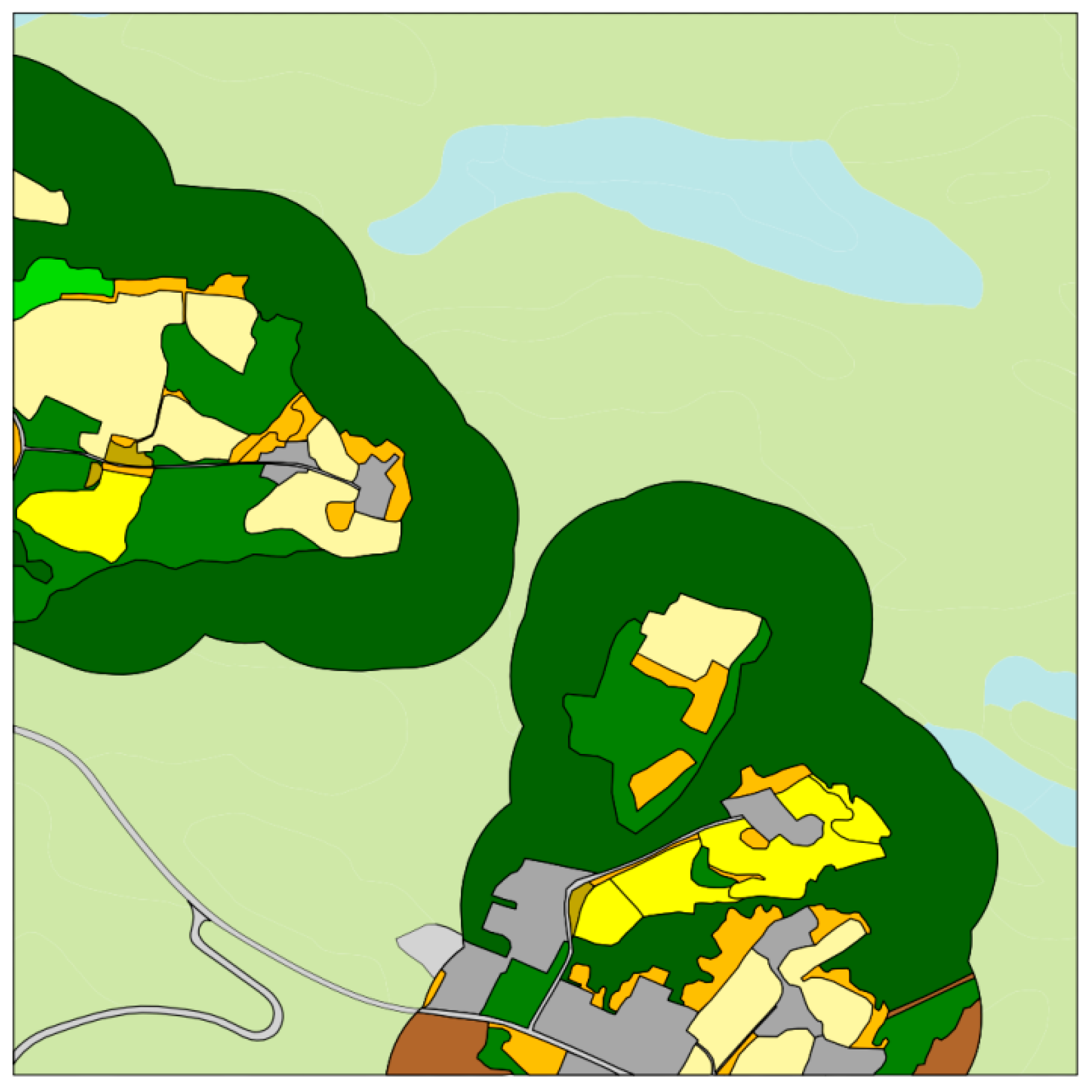
When monitoring started in 1998, the entire area of each 1 × 1 km square was mapped by 3Q staff. However, thanks to the Digital Norway project, “Area Resource Maps” (AR5) are now available for the whole country at a scale of 1:5000, and are regularly updated [22]. 3Q still provides a more detailed mapping of land use than AR5 and, importantly, a careful system of quality control that ensures that map changes reflect real changes rather than differences in interpretation of mapping rules. However, the detailed “3Q mapping” is now carried out only for the agricultural area and a 100 m wide buffer zone around this (Figure 2). Map data for the remainder of the landscape are acquired through an overlay with AR5 maps. This has considerably reduced the time spent on mapping.
2.6. Changes to Mapping Instructions
Due to the increased interest in marginal agricultural areas, several new classes have been added to the map interpretation. Primarily, these provide more detail about the percentage cover of trees and bushes on pasture and unmanaged semi-natural grasslands. In addition, a new class “outfield grazing” was added, to capture land types that are not farmland but are grazed. Improvements in time-efficiency had already been achieved with the increased experience of the mapping staff, particularly due to greater familiarity with the mapping instructions and data handling routines. In addition, some simplifications to the mapping method were introduced, based on our experience, of which data proved most useful in the first round of monitoring. For example, some of the detailed mapping categories were simplified into more aggregated classes because they represented rare land types that were being aggregated anyway for reporting purposes (Table 1). Care was taken to ensure that any changes still enabled us to produce comparable data.
One of the more extreme simplifications in classification was the aggregation of land used for cereal growing and cultivated grassland into the level 3 class “cultivated land”. However, experience had shown that interpretation of different crops, although easy later in the growing season, was very difficult based on photographs taken early in the season. In particular, newly sown land could not be attributed to either category, making analysis of these classes very difficult. Now, with advances in geographical information systems and improvements in official databases we can supplement the 3Q mapping with information about the agricultural production on the farms that have land within each monitoring square. While we do not have an exact match of which crop is grown on which fields, the agricultural statistics give us a good indicator of the types of agriculture in each sample square, and provide more useful information than the previous uncertain interpretation of crops from the aerial photographs. Official farm maps are already used in Norway as the basis for farmer applications for acreage support, such that associating applications directly to individual fields would be a feasible improvement to provide more detailed, geo-referenced management information in the future.
3. Results
3.1. Comparison of the New and the Old Data Sample
To ensure continuity of monitoring data, the first year of mapping of the new squares corresponds as far as possible with the second year of mapping of the old squares (where aerial photographs were available) and at the same time a “third” time snapshot was added. While the data from the first five-year period come from a different set of squares than the data from the second five-year period, the results for both periods are scaled up to county level and are comparable. We expect the results from the second five-year period to have somewhat higher levels of uncertainty for central farming landscapes where the number of sample squares has been reduced, but lower levels of uncertainty for marginal farming landscapes, meaning that overall there is a more even level of uncertainty across different types of agricultural landscape.
The information in Figure 3 and Table 2 is based on data from monitoring squares from two types of areas. Region 1 consists of counties where we map fewer squares in the new sample, including Rogaland in the south west of Norway and Østfold, Akershus, Oslo, and Vestfold in the South-East. Region 2 consists of counties where the agricultural area is often both smaller and more scattered, where we map a larger number of sample squares in the new sample. Region 2 includes Telemark in the South of Norway and Hordaland and Sogn og Fjordane on the West coast.
3.2. Comparison of Mapped Area
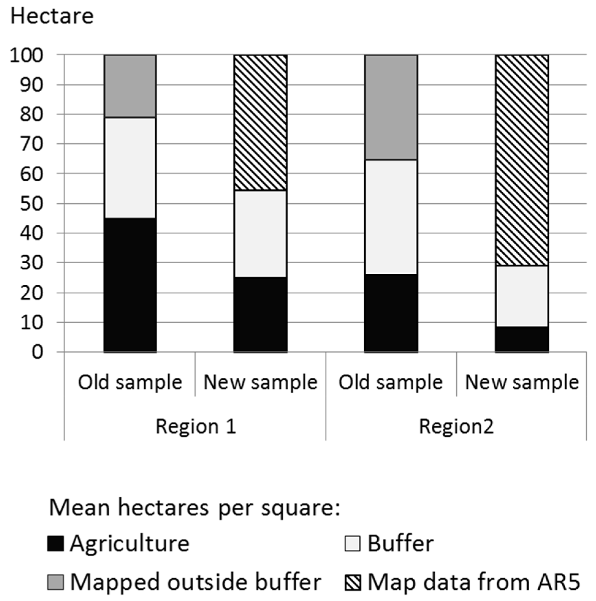
The fact that the new sample includes many squares with only small amounts of agricultural land means that the 3Q-mapped area per square is, on average, smaller in the new sample than the old (Figure 3). The total area of agricultural land plus buffer zone in these two regions was only 67% of the area covered by the old sample.
In Region 1 where we have a relatively high share of agricultural land (by Norwegian standards) the number of monitoring squares has been reduced by 45%, from 275 squares to 155. The area of agricultural land plus buffer zone was reduced by 31%. In Region 2, the number of squares has increased by 50%, from 121 to 181, but the total area of agricultural land plus buffer zone still declined by 45%.
3.3. Comparison of Results from the Old and New Samples
The results from the 3Q sample squares are scaled up to provide national and regional estimates of status and change. In the old sample, the weighting factor used to calculate regional estimates was unique to each square, and was a function of both the amount of agricultural land within the square in the first year of monitoring, and the share of agricultural land that was mapped at the regional level. Thus, squares with very little agricultural land had high weightings, to compensate for their low probability of being included in the sample. In the new sample, all squares have an equal probability of being included in the sample and the weights used to estimate regional statistics are calculated as the sum of the agricultural area of squares that fall within the region, divided by the total area of agricultural land in the region. Thus, weights for observation i (wi) vary slightly between regions, but are the same for all squares within a region.
Uncertainty is measured by the standard deviation of the total occurrence of different elements in each region (Table 2). The standard deviation is estimated using bootstrapping, where n is the sample size from the region. Bootstrapping is done by drawing n observations from the original sample with a probability of choosing observation i (pi) as
Table 2 shows the total number, length or area of elements based on the observed sample and the standard deviation of this estimate calculated using bootstrapping with resampling 2000 times. In general, larger samples are likely to reduce variation. The share of mapped agricultural land is also likely to influence the variation. In the new sample, a large mapped area in any given square results in lower wi for all squares in the region. Thus, the estimate is influenced less by any single square.
In Region 1 we have monitored fewer squares and less area per square, therefore the general trend is an increase in uncertainty from the old to the new sample. In Region 2, where we increase the number of sample squares, but map less land in total, the changes in standard deviation are more mixed. Overall, the new sample results in a more equal level of uncertainty for the two regions and avoids the extreme values that could occur in the old sample due to the effect of squares with very little agricultural land that were heavily weighted.
3.4. Landscape Changes Recorded by the Monitoring Programme
While there is considerable uncertainty around estimates of total numbers, lengths and areas of different landscape elements, the focus of the monitoring is actually not the estimates of total stocks, but rather indications of trends of change. In this section, we describe some of these results.
Net loss of agricultural land, due to either abandonment or conversion to other uses such as infrastructure, was measured to 1.5% over five years in the first round of monitoring. However, there was large variation across Norway. There were some regions where more land was cultivated than the area being abandoned. In other regions, the area under agriculture was very dynamic, with both large areas going out of production and large areas brought into production, although usually with an overall net loss of agricultural land in productive use. Regions where agriculture declined included Northern Norway, the forest region of southern Norway and the coast of western Norway. These are areas where agricultural census has shown declines in number of farms and the farmed area over several decades. In the second round of monitoring, both the losses and gains of agricultural land, as well as the overall net loss, were smaller. However, the differences between regions followed the same pattern as in the first round of monitoring.
Before the start of the monitoring programme, drainage of small streams and removal of farm ponds in the agricultural landscape were common and encouraged. The monitoring programme documents that the loss of such elements in recent times has been quite small. Existing elements have been maintained and new open ditches and ponds have been created. Loss of landscape elements was low in both rounds of monitoring. This suggests that policies to preserve and improve landscape elements, such as the compliance rules associated with agricultural subsidies, have been successful. In spite of this conservation of landscape elements, the agricultural landscape is slowly changing. For example, the sizes of arable fields have tended to increase. The growth in field size has been larger in regions that already had larger fields, increasing the difference between regions with respect to field size. Thus, the areas of Norway with the most intensive, large-scale farming have become even more intensive, while landscapes with smaller, scattered fields have been unable to follow the same trend and become relatively less efficient to farm.
3.5. Reporting Results
Results from the monitoring programme are presented at an annual open seminar, to which Norwegian agricultural authorities, County Governor’s Offices, researchers, farmers’ organisations and other interested parties are invited. Norwegian reports are all freely available in pdf–format online, and tables and figures based on the data are also sent to other institutions on demand, such as to the Norwegian Agricultural Authority for use in their reports about agriculture.
When 3Q was established, the aim was to produce objective, scientific information about how the landscape changed over time. It would then be up to the politicians to decide whether the type and direction of change was considered positive or negative. However, the Ministry of Agriculture and Food, as funders of the project, have increasingly requested not just results from the monitoring, but also opinions on the desirability of observed status and trends. The most objective way to do this is to assess monitoring results against stated national and regional agri-environmental goals. For example, the exaggerated differences between large-scale farming regions and more marginal areas suggest that policy changes may be needed to ensure that the national goal “to preserve agricultural activity throughout the entire country” is upheld. Opinions are also requested about policies that may have unintended landscape effects. An example of this may be subsidies for tree planting on former agricultural land, a “climate policy” designed to increase carbon sequestration, but that may have unintended effects on landscape character and aesthetics.
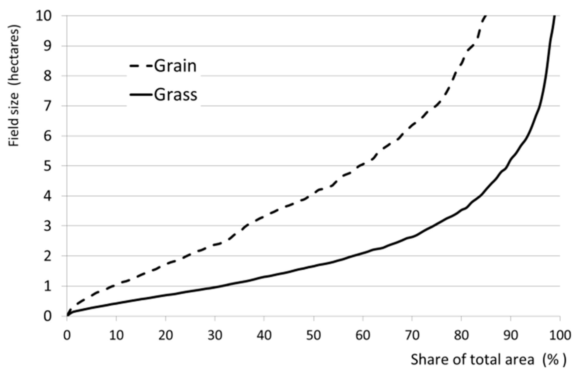
Since the start of the 3Q Programme, results have been presented in many different formats. Typically, map data initiate more discussion with and among stakeholders than data in tables. However, the exact method of expressing results can also be extremely important in influencing the degree of interest shown in the results. For example, when field sizes in Norway were expressed as average size per county there was little interest from stakeholders in this topic. However, when expressed as a graph that illustrated how much of the fully cultivated land was under or over a particular size (Figure 4), the topic was suddenly of great interest.
4. Discussion
4.1. New Sample
Since the new sample is a true random sample of agricultural landscapes in Norway, it would be possible to reduce or increase sampling density. A reduction would obviously decrease the certainty of estimates, whilst an increase would improve accuracy and would be particularly valuable for gaining more information about phenomena that are relatively rare. Although it would be preferable to obtain complete national coverage within a single season, a five-year inventory cycle has been selected based on logistical and financial constraints. Due to the large area to be sampled, the short time available to take aerial photographs and the frequent poor weather that disrupts flying plans, completing the inventory in a shorter time would not be feasible, although this may change in the future as satellite information improves (see below). The length of the monitoring interval must also respect that the Ministries funding the programme are keen to receive annual reports in order to gain continuous feedback on agricultural landscape change, thus enabling the rapid detection of new trends of change.
One issue that some countries struggle with in monitoring, is access to land, which may also be a reason for changes to a monitoring sample [10]. The main strategy of monitoring from aerial photographs avoids this problem for 3Q. However, even for the field-recording squares, there have been only very few issues with access. Every year, a letter is sent to all farmers owning land in the monitoring squares that will be visited, to inform them that people will be carrying out fieldwork. The only times farmers have made contact has been to warn of the presence of livestock. This spirit of acceptance may be due to the long tradition of “right to roam” [23] and to the generally high level of trust in Norwegian society [24]. We also emphasize that the monitoring results will only be presented in regional statistics and not associated with individual farms.
4.2. Monitoring through Use of Aerial Photography
In all mapping based on remote sensing, errors in classification are bound to occur and interpretation accuracy should be quantified. As monitoring continues for a specific area, the mapping accuracy is likely to increase, as historical information aids the interpretation of newer photographs. Finding a balance between mapping detail and accuracy is important for both the efficiency of a monitoring programme and its value for various users.
A study of the effect of fieldwork on interpretation accuracy has shown that, provided picture quality is good, field experience has little effect on accuracy [25]. In that study, ‘field trotters’ produced correct classifications in 58% of the cases whilst cartographers had an accuracy of 62%. For sampling programmes such as 3Q, costs associated with field visits to widely spread sample-squares can also be limiting.
As a supplement to aerial photography, satellite data from Sentinel (https://sentinel.esa.int/) are now opening new opportunities. Although the spatial resolution of the satellite data (10 × 10 m pixels) is not detailed enough for 3Q-mapping of landscape elements, the temporal resolution is far superior to aerial photographs. By using pixel-based analyses of multiple images, it is generally possible to extract multiple cloud-free observations throughout the growth season. We are currently working to develop algorithms for detecting clear-felled forest, new building areas, and to distinguish arable land from permanent grassland based on the pattern of development of vegetation indices through the season. These data, used in combination with the 3Q-maps, offer considerable added value, including the possibility to add information about annual changes in management of land parcels.
4.3. Communicating Results
Indicators are widely used today [26,27,28] and when calculated consistently are clearly of use in comparing status and trends from place to place and over time. Nevertheless, indicators attempt to convey simple information on very complex matters and there are risks of both oversimplification and interpretational errors [29,30]. In our experience, very few stakeholders are interested in reading about how data are collected and the limitations of the methodology. Yet these details can be important for interpreting indicators. At the other extreme, a highly simplified indicator, such as “positive or negative change for biodiversity”, does not provide enough information to assess why changes are happening or how they might be reversed or strengthened.
As an example, a stakeholder might consider that “number of habitat islands in fields” is a simple, straightforward indicator, reflecting availability of habitat for farmland biodiversity. However, habitat islands “disappear” for different reasons. They might be removed by a farmer to improve access for farm machinery, a temporary boggy patch one year might have dried out by the next round of monitoring, or a new connection to nearby forest might mean that the patch no longer fulfils the definition of “an island”. Or the entire field might have become a car park… or a forest. The consequences for biodiversity of the different types of change are very different and a GIS analysis is needed to determine the fate of each habitat island and summarize in national and regional statistics. How to present the data thus becomes a balance between presenting a simple story that is easy to understand, whilst still providing enough information to highlight causes of change and enable a discussion about possible measures to change future trends.
When vying for interest with many other news items, timing is also critical when presenting monitoring results. A short article on one specific landscape variable that can be associated with a topical political issue, will receive far more attention than an entire report on landscape status and change. Indeed, thorough reports often seem far less effectual in communicating with stakeholders than simple fact sheets on a few well-chosen topics.
Presenting results in a short article can be a challenge. We are often asked to provide tables with percentage changes. However, Norway is a country with large variation in natural conditions for farming. Some landscape elements, such as stone walls, occur regularly only in part of the country. Thus, the spread in indicator values across Norway is often large. This is important to have in mind when policies are designed. Percentage changes observed locally may seem dramatic viewed in isolation but may be of very minor significance when seen in the context of national variation. Thus, figures showing percentage change in occurrence may often give a very different impression than comparing absolute changes per county or number or length per unit of agricultural area.
The aim when developing 3Q was to establish national figures, to compare trends in Norway with those in other countries. It is clear that many countries, especially in Europe, are concerned about loss of high nature value agricultural habitats, both through abandonment and intensification [9]. However, although indicators from 3Q have been reported internationally [31], comparison with other countries is difficult since few have comparable data. However, for the development of Norwegian agricultural policies, regional information is more important, especially since today’s agri-environmental schemes are managed by the county authorities. Thus, it is at the county level we have registered the most interest in our results, even though some of the county figures are based on relatively few observations. This interest is probably due to the regional agri-environmental support program, where farmers are eligible for payments if they manage land in certain ways. These measures were originally designed and implemented at the county level. Over time, the measures have become less varied and the latest revision implemented in 2013 resulted in the same list of possible measures in all counties. However, the payments per unit area, per animal or per cultural heritage location are still decided at the county level by allocating the county budget to the various measures.
The variation across the country is for many indicators better visualized by comparing data from different landscape regions rather than the administrative regions. These are regions with more similar landscape and growing conditions. Often one county contains several landscape regions and the same landscape region may stretch across several counties. Thus, division by landscape regions is interesting from a national point of view, but less interesting at the county level, since there are too few squares at this level of division.
4.4. More Inclusive Definition of Agricultural Landscapes
With the new set of sample squares, 3Q now provides data for a broader range of agricultural landscape types than in the first years of the programme, because landscapes with only small and scattered agricultural fields are now included on equal footing with landscapes dominated by agricultural land. Nevertheless, there are still some landscape types associated with agriculture that are poorly represented, in particular the “outfields”. These are areas of rough grazing in the forests, mountains, moors or heathland. The outfields are not included in the usual definitions of “agricultural land” and are often remote from the farm, cultivated land and infield pastures. The agricultural usage of such land is poorly mapped and, being very low intensity grazing, is difficult to identify from aerial photographs. For this type of landscape, a separate monitoring programme has been established, also based on sampling of squares from the same grid as the new 3Q sample but based on field recording rather than aerial photographs. The realization that stakeholders are generally not interested in methods, enables us to present more comprehensive results about landscape change in different types of landscapes, drawing on various data sources.
Similarly, it should be noted that collection of data based on fieldwork, such as observations of birds, cultural heritage and vascular plants, are still carried out on a sample of squares from the old 3Q sample. Long time-series of species data are very rare, and this data was considered too valuable to interrupt the time-series by moving to new sample squares. Therefore we will continue to map the monitoring squares with field data, in order to analyze factors such as the relationship between birds and landscape structure [17]. Indicators from this work will also be included under the general heading of landscape monitoring.
5. Conclusions
The Norwegian 3Q monitoring programme has been running for 20 years, providing information about Norwegian agricultural landscapes. 3Q has raised awareness of landscape issues in Norway and has contributed to the development of national and regional agri-environmental programmes. The methods chosen for data collection have proven effective and efficient, and the aerial photographs provide a valuable record of agricultural landscape content and composition that can be referred to and analyzed in new ways in the future. Advances in technology and the development of other official databases have increased the amount of data available and brought down the costs of monitoring.
Author Contributions
Many people have contributed to the conceptualization, methodology and acquisition of funding for the 3Q Programme. W.F. was daily manager of the Programme from 2000–2008, G.S. from 2008 to the present. W.F. and G.S. both contributed substantially to the conceptualisation of this paper, choice of analyses and figures. W.F. wrote the first draft. G.S. did the bootstrap analysis and prepared the tables. Both contributed to the editing and reviewing.
Funding
This work was co-funded by the Norwegian Research Council grant number 194051, and the Norwegian Ministry of Agriculture and Food. The APC was funded by NIBIO.
Acknowledgments
We would like to thank colleagues at NIBIO for their contribution to the 3Q monitoring programme, especially Kristin Bay, Frode Bentzen, Karsten Dax, Wenche Dramstad, Gunnar Engan, Anne B. Nilsen, Svein Olav Krøgli, Geir-Harald Strand and Hanne Gro Wallin. We also thank three anonymous reviewers for their helpful comments and suggestions.
Conflicts of Interest
The authors declare no conflict of interest. The main funder of the monitoring programme, The Ministry of Agriculture and Food, had some influence in the programme design, as explained in the paper. However, they play no role in the collection, analyses, or interpretation of data; in the writing of the manuscript, or in the decision to publish.
References
- Council of Europe. The European Landscape Convention. European Treaty Series No. 176 2000. Available online: https://www.coe.int/en/web/conventions/full-list/-/conventions/treaty/176 (accessed on 31 January 2019).
- Herzog, F.; Franklin, J. State-of-the-art practices in farmland biodiversity monitoring for North America and Europe. Ambio 2016, 45, 857–871. [Google Scholar] [CrossRef] [PubMed]
- Wascher, D.M. (Ed.) The Face of Europe—Policy Perspectives for European Landscapes; ECNC Technical Report Series; European Centre for Nature Conservation: Tilburg, The Netherlands, 2000. [Google Scholar]
- Norton, L.R.; Maskell, L.C.; Smart, S.S.; Dunbar, M.J.; Emmett, B.A.; Carey, P.D.; Williams, P.; Crowe, A.; Chandler, K.; Scott, W.A.; et al. Measuring stock and change in the GB countryside for policy—Key findings and developments from the Countryside Survey 2007 field survey. J. Environ. Manag. 2012, 113, 117–127. [Google Scholar] [CrossRef] [PubMed]
- Cooper, A.; McCann, T.; Rogers, D. Northern Ireland Countryside Survey 2007: Broad Habitat Change 1998–2007; Northern Ireland Environment Agency: Belfast, Ireland, 2009. [Google Scholar]
- Kienast, F.; Frick, J.; van Strien, M.J.; Hunziker, M. The Swiss Landscape Monitoring Program—A comprehensive indicator set to measure landscape change. Ecol. Model. 2015, 295, 136–150. [Google Scholar] [CrossRef]
- Riedel, S.; Meier, E.; Buholzer, S.; Herzog, F.; Indermaur, A.; Lüscher, G.; Walter, T.; Winizki, J.; Hofer, G.; Ecker, K.; Ginzler, C. ALL-EMA Methodology Report: Agricultural Species and Habitats; Agroscope Science No. 57/2018; Agroscope & WSL Swiss Federal Institute for Forest, Snow and Landscape Research: Zurich, Switzerland, 2018; Available online: https://www.agroscope.admin.ch/agroscope/en/home/topics/environment-resources/monitoring-analytics/all-ema.html (accessed on 8 April 2019).
- Ståhl, G.; Allard, A.; Esseen, P.A.; Glimskär, A.; Ringvall, A.; Svensson, J.; Sundquist, S.; Christensen, P.; Torell, Å.G.; Högström, M.; et al. National Inventory of Landscapes in Sweden (NILS)—Scope, design, and experiences from establishing a multiscale biodiversity monitoring system. Environ. Monit. Assess. 2011, 173, 579–595. [Google Scholar] [CrossRef] [PubMed]
- Oppermann, R.; Beaufoy, G.; Jones, G. (Eds.) High Nature Value Farming in Europe; Verlag Regionalkultur: Ubstadt-Weiher, Germany, 2012. [Google Scholar]
- Pascher, K.; Moser, D.; Dullinger, S.; Sachslehner, L.; Gros, P.; Sauberer, N.; Traxler, A.; Grabherr, G.; Frank, T. Setup, efforts and practical experiences of a monitoring program for genetically modified plants—An Austrian case study for oilseed rape and maize. Environ. Sci. Eur. 2011, 23, 12. [Google Scholar] [CrossRef]
- Dramstad, W.E.; Fjellstad, W.J.; Strand, G.H.; Mathiesen, H.F.; Engan, G.; Stokland, J.N. Development and implementation of the Norwegian monitoring programme for agricultural landscapes. J. Environ. Manag. 2002, 64, 49–63. [Google Scholar] [CrossRef]
- Shampine, W.J. Quality assurance and quality control in monitoring programs. Environ. Monit. Assess. 1993, 26, 143–151. [Google Scholar] [CrossRef]
- Rypdal, K.; Bloch, V.V.H.; Flugsrud, K.; Gobakken, T.; Hoem, B.; Tomter, S.M.; Aalde, H. Emissions and Removals of Greenhouse Gases from Land Use, Land-Use Change and Forestry in Norway; NIJOS Report 11/05; Norwegian Institute of Land Inventory: Ås, Norway, 2005. [Google Scholar]
- Schjalm, A. Sluttrapport om Utvalg og Estimering av Kulturlandskapsovervåking; Report No. 9/99; Statistics: Oslo, Norway, 1999. (In Norwegian) [Google Scholar]
- Dramstad, W.E.; Fry, G.; Fjellstad, W.J.; Skar, B.; Helliksen, W.; Sollund, M.L.B.; Tveit, M.S.; Geelmuyden, A.K.; Framstad, E. Integrating landscape-based values—Norwegian monitoring of agricultural landscapes. Landsc. Urban Plan. 2001, 57, 257–268. [Google Scholar] [CrossRef]
- Dramstad, W.E.; Tveit, M.S.; Fjellstad, W.J.; Fry, G.L.A. Relationships between visual landscape preferences and map-based indicators of landscape structure. Landsc. Urban Plan. 2006, 78, 465–474. [Google Scholar] [CrossRef]
- Pedersen, C.; Krøgli, S.O. The effect of land type diversity and spatial heterogeneity on farmland birds in Norway. Ecol. Indic. 2017, 75, 155–163. [Google Scholar] [CrossRef]
- Pedersen, C.; Engan, G.; Stokstad, G. Plants in the Agricultural Landscape: Relationships between Plant Diversity and Distribution in Relation to Land Use, in Biodiversity in Agriculture—Lessons Learned and Future Directions. NJF Seminar 436; Nordic Association of Agricultural Scientists: Ulvik, Norway, 2011. [Google Scholar]
- OECD Multifunctionality: Towards an Analytical Framework Organisation for Economic Co-Operation and Development, Paris. 2001, p. 159. Available online: https://www.oecd.org/tad/agricultural-policies/40782727.pdf (accessed on 8 April 2019).
- Strand, G.H.; Bloch, V.V.H. Statistical Grids for Norway. Documentation of National Grids for Analysis and Visualisation of Spatial Data in Norway; Document 9/2009; Statistics Norway: Oslo, Norway, 2009. [Google Scholar]
- Engan, G. 3Q Feltkontroll av Flybildetolking—2. Omdrev, 2004–2008; Rapport 05/2012; Norwegian Forest and Landscape Institute: Ås, Norway, 2012. (In Norwegian) [Google Scholar]
- Ahlstrøm, A.P.; Bjørkelo, K.; Frydenlund, J. AR5 Klassifikasjonssystem—Klassifikasjon av Arealressurser; 06/14; Norwegian Forest and Landscape Institute: Ås, Norway, 2014. (In Norwegian) [Google Scholar]
- Act of 28 June 1957 No.16 Relating to Outdoor Recreation. 1957. Available online: https://www.regjeringen.no/en/dokumenter/outdoor-recreation-act/id172932/ (accessed on 8 April 2019).
- Helliwell, J.; Layard, R.; Sachs, J. World Happiness Report 2019; Sustainable Development Solutions Network: New York, NY, USA, 2019; Available online: https://worldhappiness.report/ (accessed on 8 April 2019).
- Strand, G.H.; Dramstad, W.; Engan, G. The effect of field experience on the accuracy of identifying land cover types in aerial photographs. Int. J. Appl. Earth Obs. Geoinf. 2002, 4, 137–146. [Google Scholar] [CrossRef]
- OECD. OECD Compendium of Agri-Environmental Indicators; OECD Publishing: Paris, France, 2013. [Google Scholar]
- Eurostat. Online Publication: Agri-Environmental Indicators. 2015. Available online: http://ec.europa.eu/eurostat/statistics-explained/index.php/Agri-environmental_indicators (accessed on 1 February 2017).
- FAO. FAOSTAT Agri-Environmental Indicators, Land Use; The Food and Agriculture Organization of the United Nations: Rome, Italy, 2018. [Google Scholar]
- Buchs, W. Biodiversity and agri-environmental indicators—General scopes and skills with special reference to the habitat level. Agric. Ecosyst. Environ. 2003, 98, 35–78. [Google Scholar] [CrossRef]
- Brouwer, F.; Crabtree, B. (Eds.) Environmental Indicators and Agricultural Policy; CAB International: Wallingford, UK, 1999. [Google Scholar]
- Fjellstad, W. Linking Farm Management to Effects on Biodiversity and Landscape. In OECD Expert Meeting on Farm Management Indicators for Agriculture and the Environment; Organisation for Economic Co-Operation and Development: Palmerston North, New Zealand, 2004. [Google Scholar]
Figure 1.
Distribution of 3Q monitoring squares in Norway: (a) the initial 3Q sample, where each point represents the location of a 1 × 1 km monitoring square with agricultural land at its center (947 squares); (b) the new data sample, a random selection of squares containing agricultural land, regardless of whether it is at the center or not (1000 squares).

Figure 2.
Example of detailed 3Q-mapping of agricultural land (yellow) and surrounding 100m wide buffer zone (grey built-up land, green forest, brown clear-fell). Outside the buffer zone, data are acquired from Area Resource Maps (AR5).
Figure 2.
Example of detailed 3Q-mapping of agricultural land (yellow) and surrounding 100m wide buffer zone (grey built-up land, green forest, brown clear-fell). Outside the buffer zone, data are acquired from Area Resource Maps (AR5).

Figure 3.
Average area of agricultural land, buffer zone (land within 100 m of agricultural land) and other area per monitoring square in the old and new sample for Region 1 (counties with fewer monitoring squares in the new sample) and Region 2 (counties with more sample squares in the new sample). Initially land outside the buffer zone was mapped as part of 3Q. For the new sample, digital Area Resource Maps (AR5) are used.

Figure 4.
The distribution of the total area of grain crops and grass crops according to field size, illustrating that most of the grain and grass area in Norway is in small fields.
Figure 4.
The distribution of the total area of grain crops and grass crops according to field size, illustrating that most of the grain and grass area in Norway is in small fields.


Table 1.
Land types at levels 1 and 2 in the hierarchical classification system, and number of classes at level 3, during the first round of monitoring (version 2002) and third round of monitoring (version 2019).
Table 1.
Land types at levels 1 and 2 in the hierarchical classification system, and number of classes at level 3, during the first round of monitoring (version 2002) and third round of monitoring (version 2019).
| Land Types: Levels 1 and 2 | Number of Classes at Level 3 | |
|---|---|---|
| 2002 | 2019 | |
| Agricultural land | ||
| Arable land and cultivated meadow | 8 | 4 |
| Horticultural land | 6 | 3 |
| Pasture | 6 | 10 |
| Unmanaged semi-natural grasslands | ||
| Uncertain pasture/hay meadows | 4 | 11 |
| Field margins and remnant grassland patches | 4 | 10 |
| Outfield grazing | 0 | 10 |
| Natural bare ground | ||
| Bare rock, boulders and scree | 3 | 3 |
| Gravel, sand, earth and peat | 5 | 5 |
| Permanent unforested dry-land vegetation | ||
| Heaths and ridges | 8 | 8 |
| Maritime vegetation | 2 | 2 |
| Cleared forest | 4 | 2 |
| Natural wetland vegetation | ||
| Mire and other freshwater wetlands | 4 | 2 |
| Salt and brackish wetlands | 2 | 1 |
| Forest | ||
| Deciduous forest | 1 | 1 |
| Mixed forest | 1 | 1 |
| Coniferous forest | 1 | 1 |
| Built-up areas | ||
| Transport routes | 8 | 7 |
| Buildings | 8 | 4 |
| Other built-up areas | 5 | 5 |
| Storage areas, dumps and rubbish tips | 7 | 7 |
| Mineral extraction | 4 | 1 |
| Urban greenways, sport and recreation areas | 6 | 4 |
| Water, snow and ice | ||
| Freshwater | 3 | 3 |
| Snow and ice | 2 | 1 |
| Saltwater and brackish water | 1 | 1 |
Table 2.
Estimated amount (number, length or area) and standard deviation of various landscape elements in the old sample (3Q-old) and new sample (3Q-new) in Region 1, with fewer monitoring squares, and Region 2, with an increase in monitoring squares. Standard deviations of the estimates are based on bootstrapping with replacement, 2000 iterations. Bold font highlights cases with a lower std.dev. in the new sample. Data in the old sample (3Q-old) and the new sample (3Q-new) are mainly from aerial photos taken in the same year.
| Region 1 | Region 2 | |||
|---|---|---|---|---|
| 3Q-old | 3Q-new | 3Q-old | 3Q-new | |
| Number of sampling squares | 275 | 152 | 121 | 181 |
| Habitat islands in fields | 56,801 | 49,739 | 30,650 | 26,801 |
| Std.dev. | 5043 | 5061 | 5334 | 4153 |
| Farmsteads | 28,849 | 27,011 | 32,934 | 25,605 |
| Std.dev. | 1517 | 2424 | 2902 | 2505 |
| Farm ponds | 1596 | 1806 | 124 | 642 |
| Std.dev. | 352 | 426 | 129 | 221 |
| Solitary trees | 4844 | 4501 | 3518 | 4905 |
| Std.dev. | 622 | 987 | 880 | 1176 |
| Ruins of buildings | 3054 | 4626 | 6621 | 6253 |
| Std.dev. | 472 | 967 | 1145 | 1353 |
| Vegetation lines, km | 557 | 636 | 224 | 233 |
| Std.dev. | 88 | 137 | 70 | 83 |
| Stone fences, km | 4567 | 3670 | 1948 | 1243 |
| Std.dev. | 691 | 877 | 407 | 230 |
| Narrow paths, km | 3261 | 4054 | 4091 | 2073 |
| Std.dev. | 270 | 498 | 414 | 279 |
| Buildings, 1000s | 477,067 | 400,567 | 414,142 | 321,905 |
| Std.dev. | 33,725 | 48,068 | 41,933 | 32,322 |
| River, canals, small streams, km | 6789 | 8002 | 8941 | 8165 |
| Std.dev. | 480 | 672 | 815 | 790 |
| Fully cultivated, hectares | 234,047 | 226,757 | 67,137 | 67,641 |
| Std.dev. | 11,926 | 21,106 | 8885 | 8776 |
| Field numbers | 148,456 | 134,715 | 117,018 | 103,086 |
| Std. dev. | 6424 | 8938 | 11,060 | 10,180 |
| Avenues of trees, km | 302 | 135 | 68 | 16 |
| Std.dev. | 55 | 39 | 18 | 8 |
| Field size, hectares | 1.58 | 1.68 | 0.57 | 0.66 |
| Std.dev. | 0.07 | 0.10 | 0.05 | 0.05 |
© 2019 by the authors. Licensee MDPI, Basel, Switzerland. This article is an open access article distributed under the terms and conditions of the Creative Commons Attribution (CC BY) license (http://creativecommons.org/licenses/by/4.0/).
Share and Cite
MDPI and ACS Style
Stokstad, G.; Fjellstad, W. Experiences from a National Landscape Monitoring Programme—Maintaining Continuity Whilst Meeting Changing Demands and Opportunities. Land 2019, 8, 77. https://0-doi-org.brum.beds.ac.uk/10.3390/land8050077
AMA Style
Stokstad G, Fjellstad W. Experiences from a National Landscape Monitoring Programme—Maintaining Continuity Whilst Meeting Changing Demands and Opportunities. Land. 2019; 8(5):77. https://0-doi-org.brum.beds.ac.uk/10.3390/land8050077
Chicago/Turabian StyleStokstad, Grete, and Wendy Fjellstad. 2019. "Experiences from a National Landscape Monitoring Programme—Maintaining Continuity Whilst Meeting Changing Demands and Opportunities" Land 8, no. 5: 77. https://0-doi-org.brum.beds.ac.uk/10.3390/land8050077
Note that from the first issue of 2016, this journal uses article numbers instead of page numbers. See further details here.