Aboveground Biomass Distribution in a Multi-Use Savannah Landscape in Southeastern Kenya: Impact of Land Use and Fences

Abstract

Savannahs provide valuable ecosystem services and contribute to continental and global carbon budgets. In addition, savannahs exhibit multiple land uses, e.g., wildlife conservation, pastoralism, and crop farming. Despite their importance, the effect of land use on woody aboveground biomass (AGB) in savannahs is understudied. Furthermore, fences used to reduce human–wildlife conflicts may affect AGB patterns. We assessed AGB densities and patterns, and the effect of land use and fences on AGB in a multi-use savannah landscape in southeastern Kenya. AGB was assessed with field survey and airborne laser scanning (ALS) data, and a land cover map was developed using Sentinel-2 satellite images in Google Earth Engine. The highest woody AGB was found in riverine forest in a conservation area and in bushland outside the conservation area. The highest mean AGB density occurred in the non-conservation area with mixed bushland and cropland (8.9 Mg·ha⁻¹), while the lowest AGB density (2.6 Mg·ha⁻¹) occurred in overgrazed grassland in the conservation area. The largest differences in AGB distributions were observed in the fenced boundaries between the conservation and other land-use types. Our results provide evidence that conservation and fences can create sharp AGB transitions and lead to reduced AGB stocks, which is a vital role of savannahs as part of carbon sequestration.

1. Introduction

Savannahs are characterized by scattered tree cover and continuous coverage of grass-dominated herbaceous plants [1,2]. On the African continent, savannahs and woodlands play a particularly large role in the carbon cycle, and wildlife and biodiversity conservation, while providing livelihoods for a huge human population [3]. The area covered by savannahs is roughly three times larger than that of forests, corresponding to approximately 50% of the total area of the African continent. Savannahs therefore represent a major carbon stock in Africa despite having a lower carbon density compared to forests [4,5,6]. Another significant feature of the African carbon cycle is that emissions caused by land-use change are greater than fossil fuel emissions [7,8]. A large part of these emissions originates from land cover conversion of savannahs and woodlands to croplands while forests still remain an important sink [7]. Woody vegetation is mainly converted into agricultural land in response to rapid population growth [9]. In contrast to woody cover loss, widespread woody encroachment has also been observed in African savannahs [10,11,12,13]. Encroaching is particularly severe in the central interior of Africa in areas with moderate woody cover, e.g., Cameroon, the Central African Republic, South Sudan, and Uganda [12]. Species with the potential to fix nitrogen, such as Vachelia tortillis and Senegalia mellifera [11], are typical encroachers in African savannahs.

African savannahs often exhibit multi-use landscapes. They can be used for wildlife-based activities, pastoralism, subsistence agriculture, forestry, and fuelwood production, and provide other ecosystem services such as climate change regulation and water reservoirs [14]. Wildlife conservation in protected areas, such as national parks, national reserves, community conservancies, and wildlife sanctuaries, promote wildlife-based tourism [15,16], which is a significant source of income for many countries, e.g., Kenya. Through wildlife management, some savannahs have been transformed into game ranching areas with high economic growth, albeit at a significant cost to conservation [17]. On the other hand, in some cases these areas have provided funds for conservation efforts. Furthermore, savannah ecosystems are suitable for livestock grazing. Therefore, they support both wild and domestic herbivores and their potential predators [18], considering the nutritional suitability of the plants [19], and the structure, productivity, phenology, composition, and chemical attributes of the ecosystem. Uncontrolled domestic herbivore populations in protected areas threaten the conservation of wild herbivores [20]. In addition, communities in savannah areas and near conservation areas grow crops for their own use and as cash crops to support their livelihoods. Population growth and land-use policies support the expansion of agricultural activities [20] at the expense of biodiversity and wildlife conservation. Although the extraction of timber, fuelwood, and non-timber forest products contributes to the livelihood options of savannah landscape dwellers, these practices may also have a negative impact on woody vegetation structure and biodiversity.

Savannahs in Eastern Africa are extremely rich in biodiversity, with high numbers of threatened species that constitute part of the largest remaining populations of iconic wildlife left on the continent [21,22]. Many countries in this region have designated a significant portion of their terrestrial areas to biodiversity conservation, amongst them some of the world-famous national parks and reserves (e.g., Serengeti National Park in Tanzania, and Tsavo National Parks and Maasai Mara National Reserve in Kenya) [22]. Their management depends on the ownership and purpose of the conservation. A large portion of these sites are owned and managed by the government for tourism, biodiversity conservation, education, and research. Recently, private and community owned conservation areas, mainly for tourism, have increased [23]. The social and economic conditions that support their management are critical for the maintenance of wildlife within their boundaries [15]. This means that human-induced drivers have more influence on wildlife abundances than those affecting ecological processes such as changes in the size of a conservation area [15].

Megaherbivores (e.g., elephants) are often of disproportionate importance in motivating conservation actions [24]. These animals are sensitive to human impact and are most likely to survive in conservation areas. However, they impact ecosystem structure [25], shape ecosystem functions [26], and affect primary productivity and soil nutrient balance [27]. They impact habitats and the presence of other animals, even small ones such as termites [28,29]. Fences are used as conservation measures to reduce the impact of large herbivores on vegetation and human habitat [29,30,31,32]. Fencing can protect stands of dense vegetation [31,32] and mitigates human–wildlife conflicts [33]. Fences are also used to demarcate protected area boundaries. However, fencing can alter ecological processes, such as dispersal of wildlife and livestock and lead to differences in plant biomass densities in grazed and non-grazed areas [34]. The role of fencing in threatening biodiversity has been also stressed [33]. Cost associated with the construction and maintenance of fences and the conflicts occurring between protected area management and communities around fenced areas are further drawbacks [35]. Woody biomass in savannah landscapes is highly variable as a result of the various factors affecting vegetation structure. However, very little information currently exists on the biomass variations in African multi-use savannahs.

Remote sensing has a central role in understanding terrestrial carbon dynamics and in the implementation of national greenhouse gas (GHG) emission inventories and payments for ecosystem services schemes such as Reducing Emissions from Deforestation and Forest Destruction (REDD+) [36,37,38,39]. Remote sensing provides information on the extent and changes of the land-use and land cover (LULC) types, and on biomass and carbon densities. The former is typically based on LULC classification, and the latter is derived from aboveground biomass (AGB) maps. AGB maps also serve other purposes, such as natural resource management [40,41]. Optical satellite images are the most common data for LULC classification and are increasingly used in cloud computing platforms, particularly Google Earth Engine (GEE) [42]. On the other hand, airborne light detection and ranging (LiDAR, also known as airborne laser scanning, ALS) provides the most accurate remote sensing method for mapping the AGB of forests [43], but savannah, bushland, and cropland AGBs in Africa have remained less studied [44,45]. Therefore, more research on the feasibility of ALS data on AGB estimation outside forests in the African savannahs are needed.

In this study, our main objective was to assess the effect of land use and wildlife fences on woody AGB density and distribution patterns in a multi-use savannah landscape in southeastern Kenya. In this landscape, fences between conservation areas and other land-use regions are used to reduce human–wildlife conflict. More specifically, we (1) used ALS and other remote sensing data to map AGB distribution and land cover in the study area, (2) examined the effect of land use (wildlife conservation, livestock management, small-holder farming) and land cover types on AGB, and (3) studied the effect of wildlife fences on AGB patterns in the boundaries of land-use regions. We hypothesized that land use considerably affects the woody AGB distribution in the studied landscape because it drives the observed patterns of land cover, and each land cover type has a characteristic AGB density. Furthermore, fences affect the distributions and effects of wildlife and livestock, and hence, contribute to the observed woody AGB patterns.

2. Material and Methods

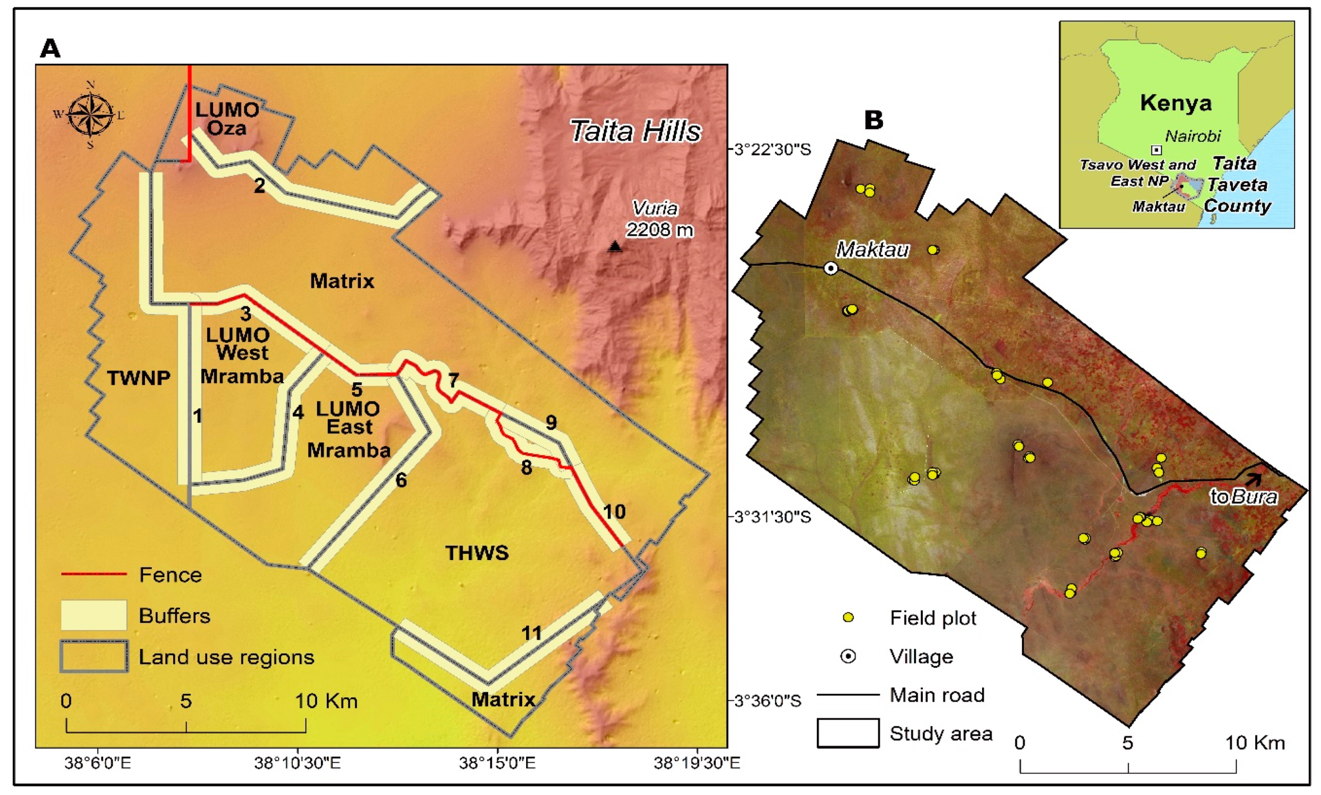
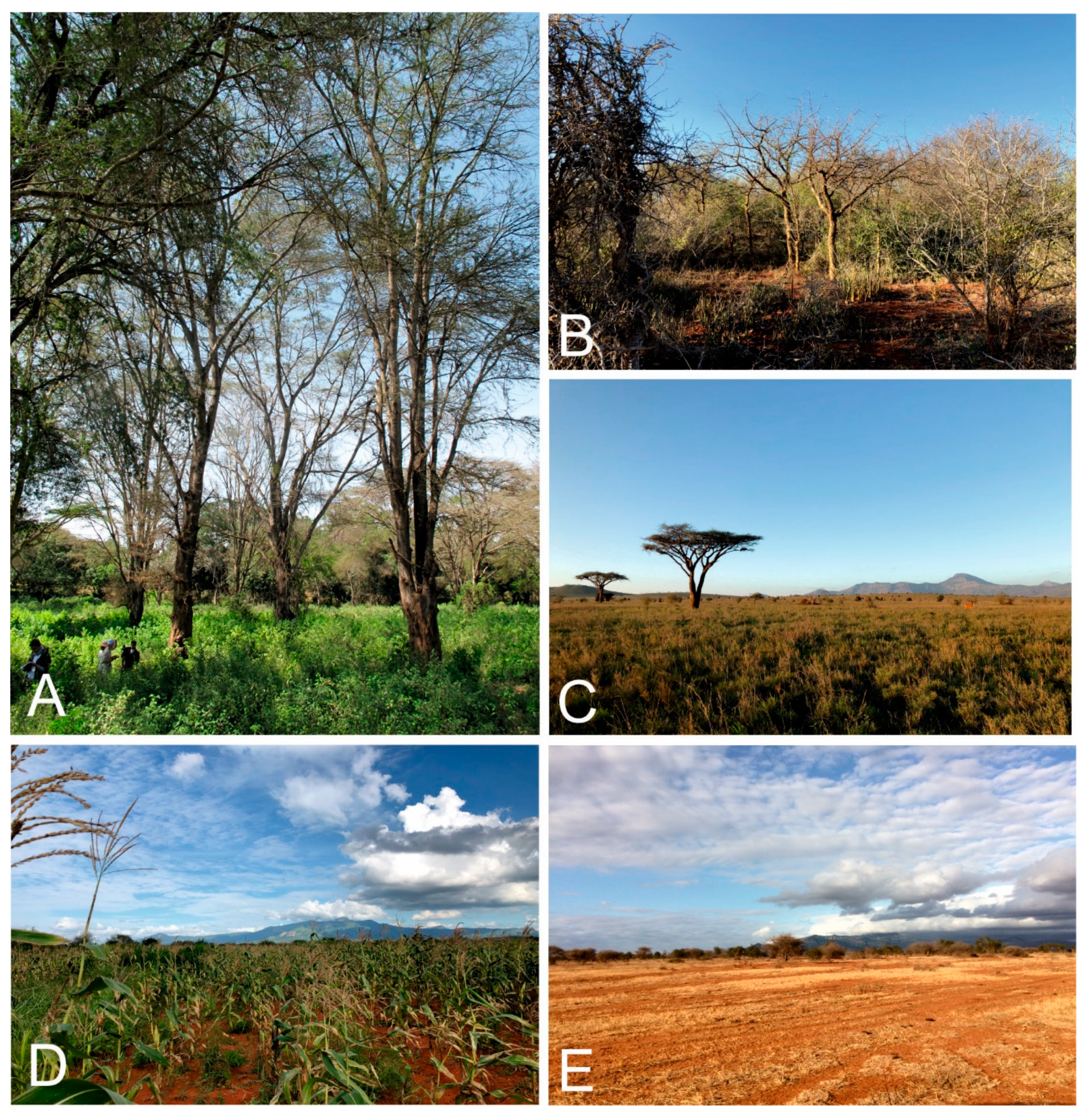
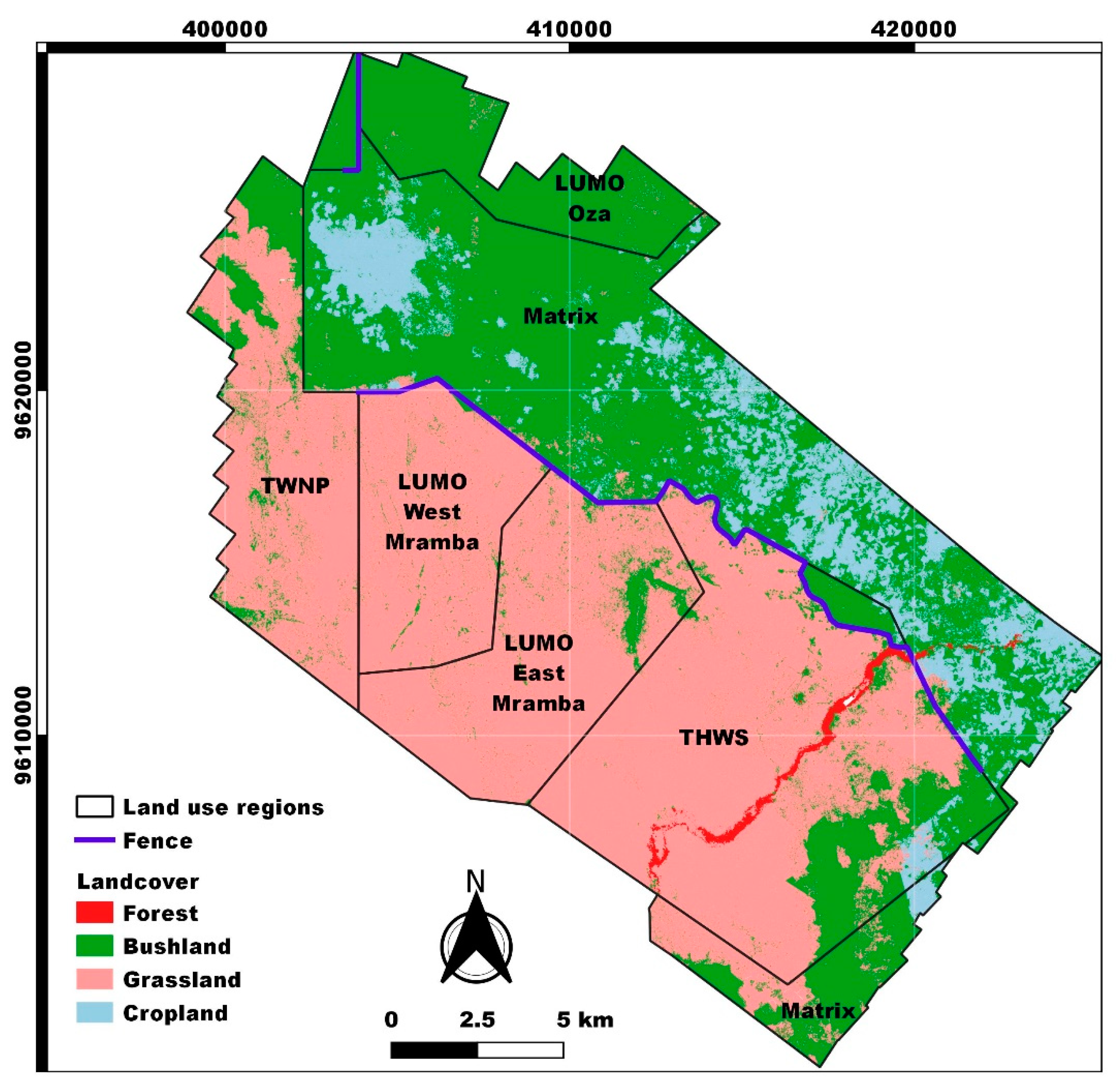
2.1. Study Area

The study area is located in the plains southwest of the Taita Hills (3°20′ S, 38°15′ E), in southeastern Kenya (Figure 1). The area belongs to Taita Taveta County. The county covers an area of 17,071 km² and has 340,670 inhabitants [46]. Typical lowland land uses include conservation in national parks, livestock management on ranches, mining, commercial sisal plantations, and dryland small-holder agriculture [6,46]. Lowland soil type is characterized by very deep, acidic, dark red, sandy clay soil (Ferralsols). Elevation ranges from 600–1000 meters above sea level (m a.s.l.) in the plains to the highest peak in the Taita Hills at 2208 m a.s.l. Average daily temperature ranges between 20 ºC and 30 ºC. Mean annual rainfall ranges from 500 mm to 1200 mm from the plains to the hills, and the rainfall pattern is bimodal with long rains in March–May and short rains in October–December [47,48]. Lowlands are much drier than highlands, e.g., the average yearly rainfall recorded at the Maktau weather station located within the study area was 483 mm in 2014–2016 [49].

Considerable variation in annual rainfall may also occur. A drought period occurred from 2007 to 2010 according to Voi meteorological station data at 580 m a.s.l., located 40 km east of the study area. The lowest annual rainfall (241 mm) was recorded in 2008 and the highest (553 mm) in 2009. The short rains in November–December 2008 resulted in only 35 mm of precipitation. The average annual precipitation was 563 mm from 2000 to 2018, while rainfall in 2006 and 2011 was 866 mm and 794 mm, respectively. As the Maktau weather station was established in October 2013 [50], we possess no rainfall data from the area of interest for the drought period, but the drought was evident. It caused a lack of water and forage for large mammals, such as elephants, which consequently caused a loss of woody vegetation, especially in conservation areas.

The Tsavo ecosystem, including Tsavo East and West National Parks (NP), cover ca. 62% of Taita Taveta County. In addition to Tsavo NPs, the Tsavo ecosystem consists of several other protected areas, namely Taita Hills Wildlife Sanctuary (THWS), Rukinga, and LUMO Community Wildlife Sanctuary, and gazetted forest patches in the Taita Hills and Kasigau Mountain. Wildlife populations (e.g., elephants, buffaloes, lions, antelopes, and giraffes) are large in the lowlands of the Tsavo ecosystem [51,52]. Cattle, elephants, and buffaloes constitute the most important herbivores and have increased from the late 1970s to date [53]. Wildlife densities may vary significantly during the wet and dry seasons. For example, 462 elephants were recorded in THWS in November 2013 during the dry season ground census, while only 17 were sighted during the wet season census in June 2013 [54]. Wildlife congregates in man-made waterholes, the Bura River, and riverine forests of THWS during the dry season, in search of water and fresh vegetation.

The study area (Figure 1) was defined by the extent of ALS data (see details in Section 2.3). The landscape includes typical lowland land-use and land cover types within THWS and a small part of Tsavo West National Park (TWNP) and LUMO Community Wildlife Sanctuary (LUMO). The three conservation areas are very different in their wildlife and livestock management. Tsavo West National Park is the largest of the three, covering ca. 9065 km², while LUMO and THWS are smaller. Although the conservation areas are managed exclusively for wildlife and wildlife-based tourism, large cattle herds may be found grazing seasonally within the boundaries. Within LUMO, the western part of Mramba (West Mramba) is preserved for livestock management, while the eastern part (East Mramba) is preserved for wildlife but is very often invaded by large cattle herds that may further invade the western plains of THWS. Cattle typically only graze in the eastern parts of THWS, while livestock occurs very seldom within TWNP. Mramba ranch holds 3500 heads of cattle and 2000 heads of goats. The entire Oza area has 3000 goats, 1500 cattle, and 130 camels, but numbers are smaller in our study site [55] and the number of livestock fluctuates between seasons and years.

Agriculture is practiced on single farms in West Mramba and in the eastern parts of THWS. Outside the conservation areas, the landscape consists of grazing land and dryland agriculture, for which the term ‘matrix’ is used here (Figure 1). The most common crops include cassava, maize, and legumes. Common woody species in the Acacia-Commiphora bushlands and thickets (Figure 2) include Vachellia tortillis, Commiphora baluensis, Vachellia xanthophloea, Albizia antihelmintica, Commiphora schimperi, Maerua angolensis, Carres tomentosa, Commiphora trothe, Senegalia mellifera, Acacia brevispica, Acacia elata, Balanites aegyptica, Boscia coriacea, Newtonia hildebrantii, Delonix elata, and Grewia villosa. The landscape is divided by the road from Voi to Taveta. A 33 km long electric wildlife fence constructed in 1999 separates the matrix and conservation areas (Figure 1).

2.2. Field Data

The field data were collected between 15 and 22 August 2018 to estimate the AGB of woody plants (trees and shrubs). The sample plots were selected subjectively to cover variation in land-use and land cover type based on high resolution satellite imagery in Google Earth, and tree cover and tree height based on ALS data (Figure 1). In total, 49 sample plots were surveyed. The field plots were positioned using a Trimble GeoXH GNSS receiver with differential correction.

The sample plot design consisted of circular plots of different sizes. The main plot was 0.1 ha in size (radius 17.84 m) and was used for inventorying all the trees with a diameter at breast height (DBH, 1.3 m height from the ground) of more than 5 cm. Height (H) for the highest, median, and shortest tree were also measured at each plot using a hypsometer (Suunto). Tree species was identified for all of these trees. Furthermore, four “subplots” of 0.01 ha (radius 5.64 m) located within the main plot were used for inventorying shrubs with DBHs of 1–5 cm (see [56] for subplot locations), and four “micro plots” of 0.001 ha (radius 1.78 m) in the central points of the subplots for measuring shrubs with DBHs < 1 cm. Shrub measurements included count, DBH, basal diameter (BD), crown diameter (CD,) and height for a median-sized shrub. The dominant woody species of each plot was also recorded.

Aboveground biomass of trees with DBH > 5 cm (AGB_trees) was computed using pan-tropical biomass model [57] due to the absence of local, species-specific allometric equations. The model (Equation (1)) is based on DBH (cm), H (m), and wood-specific gravity ($\mathsf{\rho }$, g/m³). Wood densities were obtained from a species-specific list in the BIOMASS package [58] in the R software environment [59].

$$AG{B}_{trees}=0.0673\times {\left(\rho DB{H}^{2}H\right)}^{0.976}$$

(1)

Aboveground shrub biomass (AGB_shrubs) was calculated using the equation in Conti et al. [60]. The model is based on BD (cm), CD (m), and H (cm) (Equation (2)). As BD, we used diameter at the 10 cm height (D10), which was calculated from the ground-level diameter using equation [61], as recommended in [60].

$$AG{B}_{shrubs}=\exp \left(-2.281+1.525\ln \left(BD\right)+0.831\ln \left(CD\right)+0.523\ln \left(H\right)\right)$$

(2)

Finally, we normalized AGB values per hectare and calculated the plot-level AGB as a sum of the tree and shrub AGB. Hereafter, by AGB, we refer to this aboveground biomass of woody plants unless specified otherwise.

2.3. Airborne Laser Scanning Data (ALS) and Biomass Mapping

Airborne laser scanning data were used to generate a reference canopy height model and to predict a high-resolution wall-to-wall AGB map for the study area. The scanning was conducted in late March 2014 and covered an area of 433 km². The sensor was a Leica ALS60 and a maximum of four returns per pulse were recorded. The pulse density was 1.04 pulses/m².

The data vendor (Ramani Geosystems, Kenya) pre-processed the ALS data, including filtering of the ground returns using Terrascan software (Terrasolid Oy, Finland). The data were delivered as georeferenced point clouds in the UTM/WGS84 coordinate system with ellipsoidal heights. The ground-classified returns were used for generating digital elevation models (DEM) at a 1-m cell size. The ALS point cloud elevations were normalized to height from the ground levels using DEM. Furthermore, buildings, power lines, and outliers (high points) were filtered using Terrascan, LAStools (Rapidlasso GmbH), and manual editing.

A 3.5-m height threshold provided the best model between ALS metrics and field biomass and was used to separate understory and ground returns from the canopy returns. Height metrics were calculated separately using first and last returns and canopy cover metrics using all returns (single, first, and last) (

Table A1. Summary of airborne laser scanning metrics computed using Fusion [62,63].

Predictor	Description
H.p01, H.p05, H.p10, H.p20, H.p25, H.p30, H.p40, H.p50, H.p60, H.p70, H.p75, H.p80, H.p90, H.p95, H.p99	1st, 5th, 10th … and 99th percentile of return height > 3.5 m
H.L1, H.L2, H.L3, H.L4	L-moments 1–4 of return height > 3.5 m
H.L.cv	L-moments coefficient of variation of return height > 3.5 m
H.L.skewness	L-moments skewness of return height > 3.5 m
H.L.kurtosis	L-moments kurtosis of return height > 3.5 m
H.max	Maximum of return height > 3.5 m
H.mean	Mean of return height > 3.5 m
H.min	Minimum of return height > 3.5 m
H.mode	Mode of return height > 3.5 m
H.cv	Coefficient of variation of return height > 3.5 m
H.v	Variance of return height > 3.5 m
H.stdev	Standard deviation of return height > 3,5 m
H.skewness	Skewness of return height > 3.5 m
H.kurtosis	Kurtosis of return height > 3.5 m
H.IQ	75th percentile minus 25th percentile for cell
CC.first	First returns > 3.5 m/Total first returns * 100
CC.all	All returns > 3.5 m/Total all returns * 100
CC.all.first	All returns > 3.5 m/Total first returns * 100
CC.first.mean	First returns above mean/Total first returns * 100
CC.all.mean	All returns above mean/Total all returns * 100
CC.all.mean.first	All returns above mean/Total first returns * 100
CC.first.mode	First returns above mode/Total first returns * 100
CC.all.mode	All returns above mode/Total all returns * 100
CC.all.mode.first	All returns above mode/Total first returns * 100

All height variables (beginning with ‘H’) were calculated separately using first and last pulse returns, which are indicated by the prefix ‘FR_’ or ‘LR_’, respectively. All canopy variables (beginning with “CC”) were calculated using all returns only.

). The variables included all the variables available in the FUSION software [62] and ones used in our earlier study [63]. Square root transformation was applied to AGB, as it was found to improve the linear relationship between AGB and explanatory variables. The “regsubset” function in the “leaps” package [64] was used to fit multiple linear regression models between the ALS metrics calculated from the ALS point density clipped over the field plot and the AGB calculated from that field plot. The leave-one-out cross-validation root mean square error (RMSE) and the coefficient of determination (R²) were used to select the best AGB model. The predictions were back-transformed (squared), and the square of the residual standard error was added to the predicted values to avoid back-transformation bias [45,65]. For AGB prediction at wall-to-wall level, spatial grids of ALS metrics were generated at a spatial resolution of 30 m × 30 m. Mean densities of AGB in each land-use and land cover class was calculated from the AGB map.

2.4. Satellite Imagery and Land Cover Mapping

We collected Sentinel-2 images (top of atmosphere reflectance) with cloud cover less than 20% in the images during the dry seasons [short dry season (January 1 to February 28) and long dry season (July 1 to September 30)] in 2017 and 2018, and pre-processed them in the GEE platform. In total, 103 Sentinel-2 images (bands with a resolution of 10 m and 20 m only) were used to calculate the median dry season image. Median dry season images were calculated for all bands in the blue to the shortwave infrared spectral range based on all available cloud-free pixels (Figure 1B). In addition, a normalized difference vegetation index (NDVI) [66], an enhanced vegetation index (EVI) [67], EVI2 [68], two variants of normalized difference infrared index (NDII-1 and NDII-2) [69], and an optimized soil-adjusted vegetation index (OSAVI) [70] were calculated from the median image.

Additionally, land cover classification was performed in the GEE platform. In addition to median dry season Sentinel-2 composite and vegetation indices, input data included an ALS-based canopy height model (CHM). The land cover in the landscape was classified into four land cover types (cropland, grassland, forest and bushland) according to the Land Degradation Surveillance Framework [71]. Cropland is cultivated land with annual or perennial crops, while grassland contains grasses and other herbs with less than 10% woody cover. Forest in our classification is made up of a continuous stand of trees with partly interlocking crowns, typically along the riverbeds. Bushland is made up of mixed trees and shrubs with a canopy cover of 40% or more, while thickets are closed stands of bushes and climbers usually between 2 m and 7 m tall and shrubland are open or closed stands up to 3 m tall. For this study, thickets and shrubland were incorporated into bushland because we had few field plots for those classes and the classes were similar in reflectance and vegetation characteristics.

In the first step, training data were collected through visual interpretation using ArcGIS 10.3 for the four land cover classes. The pixels for training the classifier were selected based on image interpretation and CHM. Classification and regression trees (CART) [72] were observed to obtain the highest overall accuracy among the classifiers in GEE and was thus selected for the classification. The reference data set for accuracy assessment included the 49 points surveyed in 2018 in the field, which were not used as training points in the classification. Finally, manual editing was performed in ArcGIS to address some of the apparent misclassification in the land cover map.

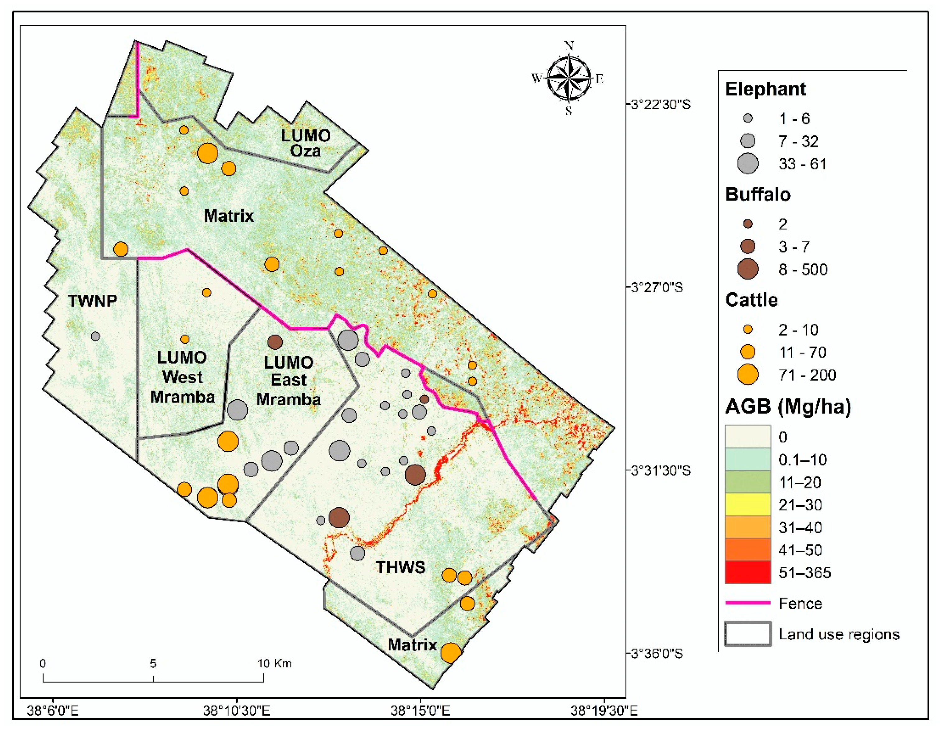
2.5. Wildlife and Livestock Data

Elephant, buffalo, and cattle data were taken from the Tsavo–Mkomazi large mammal census of 2014 to be comparable with the 2014 ALS data used. The wildlife census is conducted by the Kenya Wildlife Service (KWS) every three years to establish the status of key species in the Tsavo ecosystem. The census is carried out from fixed-wing aircrafts and the data collection procedure is described in detail in [73]. The animal spatial distribution and densities were further compared with AGB in the studied landscape (Figure 3).

2.6. Statistical Analyses of AGB Data

The plot-level AGB values were used for computing descriptive statistics (range, mean, median, and standard deviation) for the field data. The Kruskal–Wallis test was conducted to study whether differences in AGB were statistically significant between the land-use regions and land cover classes. Furthermore, median and mean values of the AGB per class were illustrated with a box plot for the different land-use regions and land cover classes. We also estimated the percentage area covered by each land cover in the respective land-use region. Finally, 500-m wide buffers were set in 11 segments of land-use region boundaries to assess local AGB differences (Figure 1A). The buffers were categorized into fenced and non-fenced segments to determine the effect of the fence on AGB. Pixel values were studied separately for two sides of the boundary by calculating the percentage of zero AGB pixels. Furthermore, medians of the non-zero AGB values were studied using the Wilcoxon test. All analyses were performed in the R statistical environment [74].

3. Results

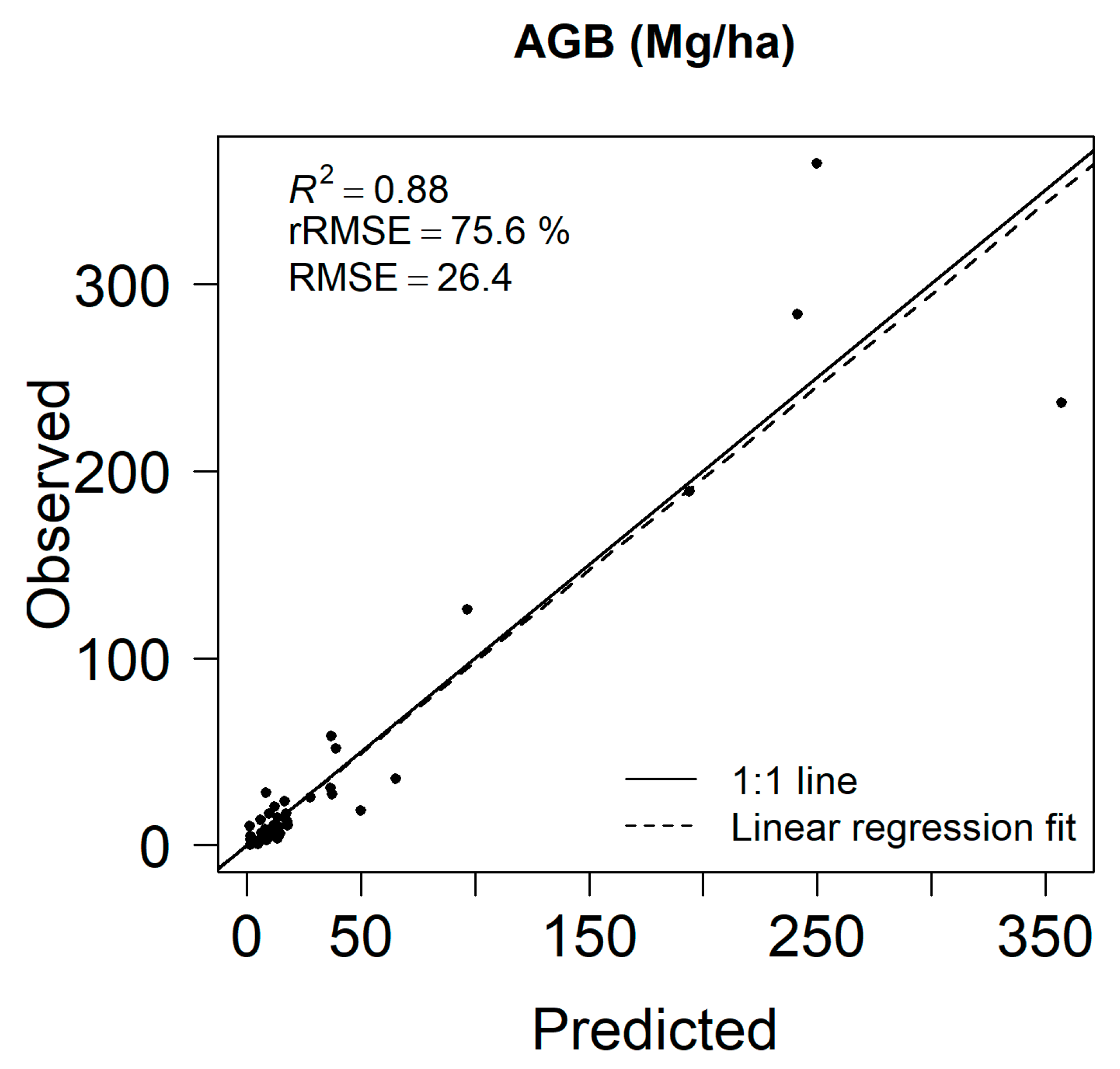
3.1. Aboveground Biomass Estimates and Map

Woody AGB estimates based on the field plot measurements are summarized in

Table 1. Summary of the aboveground biomass (AGB) values based on the field data according to the diameter at breast height (DBH) class (n = 49). AGB was estimated based on diameter at ground level for shrubs with a DBH < 1 cm. SD = standard deviation, IQR = interquartile range.

DBH Class	AGB (Mg/ha)
	Mean	Min	Max	SD	IQR	Median
DBH > 5 cm	42.15	0.28	364.04	85.41	20.94	7.91
DBH 1–5 cm	3.69	0.00	19.46	4.98	4.03	2.07
DBH < 1 cm	0.52	0.00	2.56	0.60	0.49	0.35
Total	38.02	0.00	364.54	78.27	21.56	10.04

. The maximum plot-level values are nearly 365 megagrams per hectare (Mg/ha) and were observed in the riverine forest. The plots with the lowest AGB had very little woody biomass and were located in the grassland areas.

The final modeling results for mapping AGB using ALS data are shown in Figure 3. The model was based on two variables: CC.all (percentage of all returns above 3.5 m; p < 0.001) and Elev.min.fr (minimum elevation of the first returns above 3.5 m; p < 0.001). The model performed well in terms of model fit (R² = 0.88) although RMSE based on leave-one-out cross-validation was relatively large (26 Mg/ha, 75.6% of the mean AGB). However, the model did not show any signs of systematic over- or under-estimation (Figure 3).

The AGB map shows predicted biomass density patterns at 30 m × 30 m resolution (Figure 4). The mean AGB in the study area was 5.9 Mg/ha. The Riverine forests in the southern and southeastern parts of the landscape within THWS had the largest AGB densities. We also observed relatively large AGB densities outside the protected areas towards the foothills of the Taita Hills, in the northeastern part of the landscape. Aboveground biomass spatial variations were also relatively large in the matrix and in LUMO Oza. On the other hand, the lowest AGB values were found in the nearly treeless grassland of THWS, LUMO East Mramba, LUMO West Mramba, and TWNP.

Wildlife (elephant and buffalos) and livestock (cattle) were highly evident in the conservation areas based on the 2014 KWS wildlife census. Elephants were present in LUMO Mramba East and THWS, and were absent in the matrix (Figure 4,

Table 2. Animal counts (animals) and densities (animals/km²) per land-use region during the 2014 wildlife census by Kenya Wildlife Service. Land-use regions: Taita Hills Wildlife Sanctuary (THWS), LUMO Community Wildlife Sanctuary (LUMO East Mramba and LUMO West Mramba), Tsavo West National Park (TWNP), and other land use (matrix).

Animal	Land-Use Region (area)
	TWNP (48.92 km2)	LUMO East Mramba (47.24 km2)	LUMO West Mramba (33.92 km2)	THWS (101.50 km2)	Matrix (141.63 km2)
Elephant	5 (0.10)	137 (2.90)	0 (0)	237 (2.33)	0 (0)
Cattle	0 (0)	540 (11.43)	20 (0.59)	100 (0.99)	623 (4.40)
Buffalo	2 (0.04)	7 (0.15)	0 (0)	802 (7.90)	0 (0)

). Cattle were found in all the land-use regions, except in the small portion of TWNP captured during the ALS campaign (Figure 4). Their density was highest in LUMO East Mramba (11.43 animals/km²), a portion of the landscape secured for livestock grazing and was second highest in the matrix (4.40 animals/km²), where agriculture is the most common land use. Buffalos were found in the conservation areas, showing the highest number per unit area in THWS (Table 2). We categorized the animals into three herd sizes, in which the number of animals per herd differed per animal species (Figure 4). We saw no elephants or buffaloes in the matrix during the 2014 wildlife census. Furthermore, no animals were visible in LUMO Oza.

3.2. Land Cover Classification

The overall land cover classification accuracy was 88.78%. The producer’s and user’s accuracy are shown in

Table A2. Errors of omission and commission per class in the land cover classification.

	Forest	Bushland	Grassland	Cropland	Row Total	Producer’s Accuracy
Forest	47	5	0	0	52	95.91
Bushland	1	59	4	2	66	76.62
Grassland	0	6	100	3	109	92.59
Cropland	1	7	4	55	67	91.66
Column total	49	77	108	60	294
User’s accuracy	90.38	89.39	91.74	82.08

. The land cover map shows the distribution of the land cover classes in the landscape (Figure 5). Bushland and cropland dominate the matrix in northern and northeastern parts of the landscape, while grassland that is representative of the savannah biome dominates the southern and southeastern parts (THWS, LUMO Mramba, TWNP). LUMO Oza is almost completely bushland as there is less agriculture and livestock management. Forest is the land cover type with the smallest area, located mostly in THWS along the Bura River. THWS also has relatively large patches of bushland in its eastern parts bordering the matrix. Cropland is also present in the eastern part of THWS, while it is not observed in the other conservation areas. The THWS wardens consider it a form of informal encroachment.

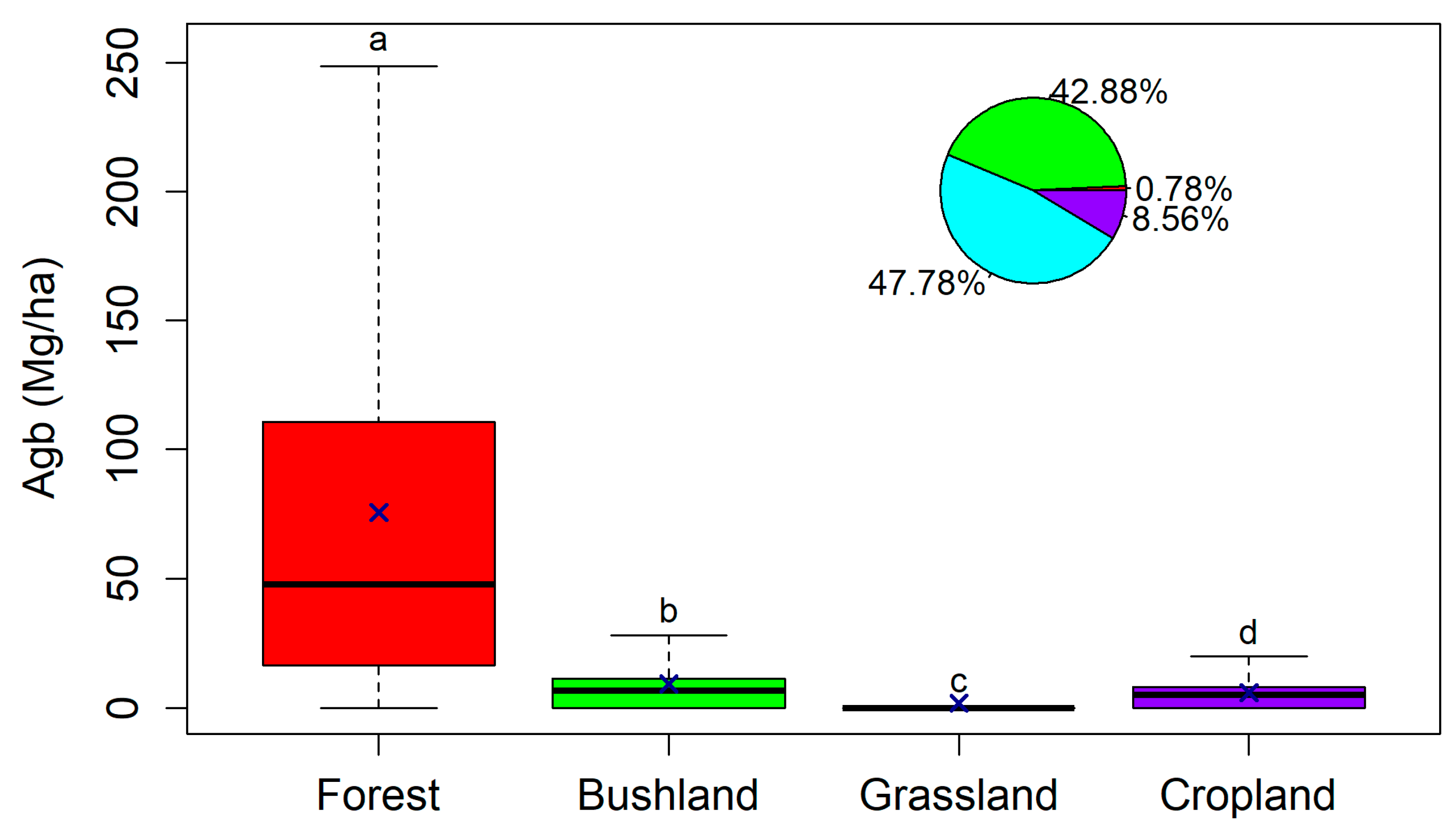
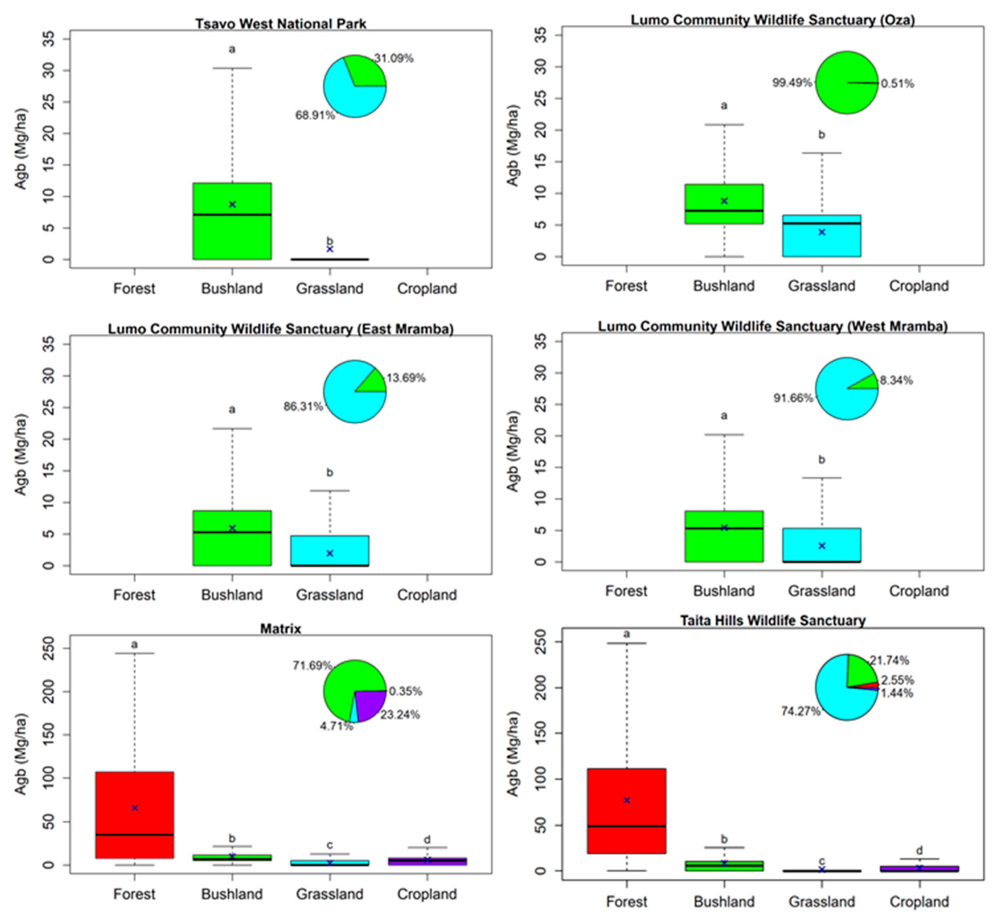
3.3. Effect of Land Cover and Land Use on Aboveground Biomass

Aboveground biomass values for the land cover types are shown in Figure 6 and

Table 3. Aboveground biomass (AGB) statistics for land-use regions and land cover types based on AGB and land cover maps. IQR = interquartile range. Land-use regions: Taita Hills Wildlife Sanctuary (THWS), LUMO Community Wildlife Sanctuary (LUMO East Mramba, LUMO West Mramba, and LUMO Oza), Tsavo West National Park (TWNP), and other land use (matrix).

Land-Use Region	Land Cover	AGB (Mg/ha)
		Mean	Min	Max	SD	IQR	Median
LUMO Oza	Bushland	8.8	0.0	82.3	7.9	6.3	7.3
	Grassland	3.9	0.0	20.1	4.4	6.6	5.2
	All	8.8	0.0	82.3	7.9	6.2	7.2
LUMO East Mramba	Bushland	5.9	0.0	106.2	7.6	8.7	5.3
	Grassland	2.0	0.0	50.9	3.8	4.7	0.0
	All	2.4	0.0	106.2	4.6	5.1	0.0
LUMO West Mramba	Bushland	5.4	0.0	104.4	6.3	8.1	5.3
	Grassland	2.6	0.0	55.6	4.2	5.3	0.0
	All	2.6	0.0	104.4	4.4	5.4	0.0
THWS	Forest	77.4	0.0	353.0	79.0	92.5	49.0
	Bushland	8.1	0	159.3	11.9	10.1	5.5
	Grassland	1.4	0	237.3	4.2	0	0
	Cropland	3.0	0.0	100.3	7.0	5.1	0.0
	All	4.8	0.0	353.0	18.6	5.1	0.0
TWNP	Bushland	8.8	0	71.8	8.3	12.2	7.1
	Grassland	1.7	0	100.9	3.4	0	0
	All	3.8	0.0	100.9	6.3	6.2	0.0
Matrix	Forest	66.0	0.0	346.7	73.8	99.3	35.0
	Bushland	9.9	0.0	353	13.3	6.6	6.9
	Grassland	2.2	0.0	54.5	4.0	5.1	0.0
	Cropland	6.0	0.0	241.3	9.4	8.1	5.2
	All	8.9	0.0	353	13.5	10.5	6.3
All Land cover	Forest	75.5	0.0	353.0	78.3	94.2	47.8
	Bushland	9.2	0	353	11.9	11.2	6.7
	Grassland	1.8	0	237.3	4	0	0
	Cropland	5.8	0.0	241.3	9.3	7.9	5.1
	All	5.9	0.0	353.0	13.1	7.6	0.0

. The forest had the highest mean AGB (75.5 Mg/ha) followed by bushland (9.0 Mg/ha) and cropland (5.8 Mg/ha). Grassland had clearly the lowest mean AGB, as it is mostly treeless (mean 1.8 Mg/ha, median 0 Mg/ha). However, bushland, cropland, and grassland also had very high AGBs at certain locations (maximum values in Table 3). These areas correspond to “forest-like” bushland with trees and large shrubs. The highest values in the cropland were found in the fallowed fields and patches of bush and in the tree-covered areas next to the fields. In addition, certain farmers practice agroforestry, meaning that they grow trees for fruit and timber production and for providing shade for crops. Furthermore, the grasslands also have scattered large trees, e.g., in Figure 2C. We observed significant AGB differences among the land cover types (p < 0.001) according to the Kruskal–Wallis mean rank test. Furthermore, the Dunn test indicated a significant difference (p < 0.05) between all the land cover types (Figure 6).

When comparing the land-use regions, the mean AGB values in descending order were 8.9 Mg/ha in the matrix 8.8 Mg/ha in LUMO Oza, 4.8 Mg/ha in THWS, 3.8 Mg/ha in TWNP, 2.6 Mg/ha in LUMO West Mramba, and 2.4 Mg/ha in LUMO East Mramba (Table 3). According to the Kruskal–Wallis test, the AGB differences among land-use regions were significant (p < 0.001). These differences are mainly explained by dissimilarities in the land cover class distributions (Figure 7). The matrix has very little grassland with low AGB, but a large fraction of bushland with a relatively high AGB. The area also has some forest and cropland with high maximum values, which increase the mean AGB. LUMO Oza also mainly consists of higher AGB bushland, while lower AGB regions have larger fractions of grassland. This includes both the West Mramba grazing area and various protected areas. We conducted pairwise comparisons between the classes using the Dunn test, which indicates a significant difference (p < 0.05) between all the classes (Figure 7).

3.4. Effect of Fences on Aboveground Biomass

Lastly, we compared AGB values in the fenced and non-fenced boundaries of the land-use regions (see Figure 1A for buffer numbers).

Table 4. Percentage of zero woody aboveground biomass (AGB) and median AGB for non-zero AGB pixels. P value refers to the Wilcoxon test results made for the non-zero AGB values. Numbers in the end of land-use region names refer to the numbers of buffers in Figure 1A.

Side 1	Side 2	Fence	Percentage Zero AGB		Median for Non-Zero AGB
			Side 1	Side 2	Side 1	Side 2	P Value
TWNP_1	LUMO West Mramba_1	No	57.6	52.9	7.1	6.6	<0.001
LUMO Oza_2	Matrix_2	No	20.7	17.0	8.2	8.2	>0.05
LUMO West Mramba_3	Matrix_3	Yes	84.3	44.1	6.5	6.4	>0.05
LUMO East Mramba_4	LUMO West Mramba_4	No	63.2	58.2	6.7	6.8	>0.05
Matrix_5	LUMO East Mramba_5	Yes	32.6	62.6	7.2	7.2	>0.05
LUMO East Mramba_6	THWS_6	No	85.9	84.9	6.5	6.9	<0.001
THWS_7	Matrix_7	Yes	75.2	22.0	6.9	8.8	<0.001
THWS1_8	THWS2_8	Yes	5.3	72.0	12.6	8.0	<0.001
Matrix_9	THWS_9	No	31.0	10.6	9.1	10.0	<0.001
Matrix_10	THWS_10	Yes	56.2	61.9	6.7	9.7	<0.001
THWS_11	Matrix_11	No	69.9	56.4	6.6	6.8	>0.05

reports the fraction of zero AGB pixels for two sides of the buffer and the Wilcoxon test results for the non-zero AGB values.

The largest differences in the percentage of zero AGB occurred in the fenced boundaries (buffers 3, 5, 7 and 8). Most of the non-fenced boundaries (buffers 1, 2, 4, 6 and 11) showed only small differences. However, a greater difference was observed in the non-fenced buffer 9, which corresponds to the boundary between bushland part of THWS and the cropland-dominated matrix. Buffer 10 showed relatively small difference in the presence of zero AGB although there is a fence. This boundary is between THWS and the matrix in the eastern part of the study area.

The medians of the non-zero AGB values differed most substantially in the fenced buffers 7, 8 and 10 (all differences highly significant according to the Wilcoxon test) (Table 4). Although percentage zero AGB was substantially higher in LUMO West and East Mramba than in the matrix in the fenced buffers 3 and 5, median AGB did not differ significantly (P > 0.05). However, smaller but highly significant differences were also observed in the non-fenced buffers 1, 6 and 9. Buffer 1 is located in the non-fenced boundary between TWNP and LUMO West Mramba, where bushland in the northern part of TWNP has a relatively high AGB compared to grassland-dominated West Mramba. Buffer 6 corresponds to the boundary between two conservation areas, LUMO East Mramba and THWS.

4. Discussion

4.1. Remote Sensing—Based Biomass and Land Cover Maps

We used field data and ALS metrics to create a wall-to-wall high-resolution AGB map. The model fit and accuracy were similar [75,76] or compared favorably with previous studies in temperate and tropical forests [65,77,78,79]. Our model was based on two predictors: minimum elevation of the first returns above 3.5 m and percentage of all returns above 3.5 m. These variables characterize canopy height and cover, both of which are related to AGB. Similar combinations of height and cover variables have also been used in previous studies in sub-Saharan Africa [78,80,81]. Field-measured AGB included both shrubs and trees. According to the field data, shrubs (DBH 1–5 cm) can make an important contribution to woody AGB. However, as a height threshold of 3.5 m was used to separate canopy and ground returns, woody vegetation less than 3.5 m in height does not affect the ALS variables. Therefore, areas where shrubs are less than 3.5 m in height appear as zero AGB in the map. We selected the height threshold from the tested values, as it provided the most accurate predictions. Further research should be conducted to map AGB variations in the smallest shrubs and grasses.

We used Sentinel-2 satellite images and the CART algorithm in the GEE platform for creating the LULC map. We achieved a good overall accuracy of 88.78% when using dry season composites. Previous studies have shown that the dry season is best suited for separating variations in woody AGB [82,83]. One topic for further research would include classifying various grassland types within the study area.

Spatially explicit AGB and LULC maps offer additional knowledge of AGB variations across the savannah landscapes compared to spatially limited field inventories. In this study, maps demonstrated the link between LULC and AGB, and sharp AGB gradients in certain boundaries of the land-use regions. Furthermore, maps enable geospatial analyses of the AGB patterns, e.g., together with wildlife and livestock inventories, and can inform land management interventions [45]. In our study, maps showed that grassland concentrated in the wildlife conservation areas, where AGB was reduced due to the browsing effect on trees [83]. As there are fewer large mammals outside the conservation areas, their negative impact on woody vegetation is less in these areas. Therefore, wildlife and livestock frequency in the multi-use landscape contributes to the low biomass densities in the region.

4.2. Effect of Land Cover and Land Use on Aboveground Biomass

Our results reveal a significant difference (P < 0.05) in woody AGB among the land cover and land-use classes in the studied landscape. In general, AGB is concentrated in areas with larger tree densities. According to the field data, shrubs and smaller trees can also have a considerable effect on woody AGB density. We observed the highest AGB densities in the forest along the Bura River Valley and towards the foothills of the Taita Hills, while grassland had the lowest AGB densities. As the forest class only occupies a small area, other land cover classes contributed more to the total AGB stock at the landscape level. This emphasizes that a greater amount of AGB is stored in open savannah and bushland than in the forest. Bushland occupies more than half of the total area, and therefore contributes the most to the total AGB stock. The contribution of cropland to the total AGB in the landscape is due to agroforestry (i.e., trees growing on cropland). The mean AGB densities in the landscape were low compared to montane forest, exotic plantation, and woodland in the higher altitudes of the Taita Hills [65,84]. Furthermore, biomass in the bushland was comparable to the leaf biomass of sisal (Agave sisalana) in a commercially owned plantation established in the savannah landscape in Taita Taveta [85]. Low precipitation [39,86], small-scale farming by resource-poor farmers [87], low CO₂ concentrations in arid and semiarid regions [88], and disturbance from fire and herbivores [89,90] are among factors responsible for the generally low AGB in the savannah landscape.

We categorized the multi-use savannah landscape into conservation (TWNP, THWS, and LUMO) and non-conservation areas (matrix) based on land use. Furthermore, the conservation types were categorized based on ownership and management. The TWNP, LUMO, and THWS are government, community, and privately owned and managed, respectively. The AGB differences between land-use regions are driven by the land cover differences. We observed the highest woody AGB densities in non-conservation areas (matrix), which are mainly bushland and cropland, while LUMO West Mramba and LUMO East Mramba, community owned and managed wildlife sanctuaries that are mainly grassland, showed the lowest mean AGB densities. THWS and TWNP had similar mean AGB densities, while LUMO Oza had a much higher AGB compared to grassland-dominated regions because of its larger fraction of bushland.

Our results support the hypothesis that there is a link between the land use (conservation and non-conservation) and dominant land cover type, which affect the observed AGB patterns. Presence of wildlife is important for grassland to remain sparsely wooded, and hence, wildlife conservation contributes to open grassland with relatively low woody AGB. Furthermore, ranches for livestock contribute to the low AGB. THWS and LUMO West Mramba serve as a migratory corridor for elephants moving between Tsavo West and Tsavo East NPs in search of food and water [51]. Contrary to the February 2011 elephant census [73], the elephant density in the region increased from less than 0.5 elephants/km² in 2011 to > 2 elephants/km² in February 2014. This considerable increase in elephant population contributes to low AGB densities in the region. Habitat improvements through water supplementation in the protected areas also attract wildlife and further create pressure on the vegetation. Waterholes attract large congregations of herbivores particularly during the dry season [73]. Williams et al. [91] have also suggested the presence of surface water acts as a determinant of the distribution of water-dependent wildlife species. The wildlife and livestock census data also showed that private (THWS) and government (TWNP) owned conservation areas had more wildlife (elephants and buffalos) while the community owned conservation areas attract more livestock. This could be associated with the management strategies employed by the respective agencies. Therefore, policies and management strategies geared towards woody vegetation protection should be introduced into wildlife conservation management plan in order to reduce AGB decline in conservation areas.

Recent studies in the same region show that conversion of bushland to treeless cropland [92] increases land surface temperatures and decreases evapotranspiration, and low tree canopy cover areas cause higher land surface temperatures and higher temperatures in general [93]. Together with increasing proportion of agricultural areas, conservation areas have a negative contribution to the local climate, and furthermore, to the regional climate. Furthermore, bushland protection is vital for the conservation of flora and fauna, and for habitat conservation [91,94]. Furthermore, high AGB bushland supports, for example, the mitigation of wildfire, poor water quality, soil erosion, soil PH, air temperature and other ecosystem services of importance to the ecology, climate and wildlife [91,92,95]. Restoration of degraded areas by fencing, enrichment planting of woody plants and translocation of wildlife (browsers) to high biomass areas, agroforestry, and sustainable environmental regulation are some ways to mitigate these effects. Therefore, the trade-offs between the wildlife conservation and benefits of woody vegetation should be considered carefully in the conservation area management and land-use planning.

Although not addressed in this study, in addition to land use, natural factors, such as soil type, ground water table level, and rainfall, may contribute to land cover and AGB patterns. The soil type is typically red laterite, but parts of the landscape are characterized by sedimentary carbonites, which are drier and less fertile soils, thus introducing sparser woody vegetation. The water table level is high, especially along the Bura River Valley, enabling better tree growth. Furthermore, rainfall and mist emergence in topographically higher areas, such as Maktau Hill in LUMO Oza, may increase tree cover and height. Further studies should aim to clarify the roles of land use and natural factors on land cover and AGB in the study area.

4.3. Effect of Wildlife Fences on Biomass Distribution and Density

Fencing conservation areas is primarily done to prevent wildlife from intruding into surrounding communities and farmlands, in other words, to reduce human–wildlife conflicts [96,97,98,99]. Fences additionally help minimize wildlife poaching and the illegal extraction of other vital resources from protected areas [33] and hinder the transmission of vector-borne diseases between livestock and wildlife, as production animals and wildlife are kept separate. In Kenya, 60% of all protected areas are fully or partially fenced [35].

The ecosystem in the Taita Hills lowlands faces challenges, including livestock incursion, poaching, drought, land-use change, human–wildlife conflict, unprescribed fires, invasive species, and vegetation damage by elephants [100]. Electric and non-electric fences have therefore been constructed on the borders of the protected areas to minimize some of these challenges. The fence from Maktau to Bura Village was built in 1999 [33]. It restricts the movement of wildlife from conservation areas and hinders unauthorized access to the areas [99]. Fences also protect degraded habitats and support forest regeneration trials. Furthermore, fences around farms restrict wildlife and livestock from entering the farms.

According to our analysis of the AGB variation in the boundaries of the land-use regions (buffers), the largest differences in the percentage of zero AGB and median AGB occurred in the fenced boundaries. In the buffers 3, 5 and 7, which correspond to the boundary between the conservation areas (LUMO West and East Mramba, THWS) and the matrix, the percentage of zero AGB was considerably higher in the conservation area sides of the fence. The zero AGB pixels refer to pixels without any woody AGB, which may indicate large pressure from herbivores on woody vegetation. This is supported by the high density of wildlife close to the fence in LUMO East Mramba and THWS (Figure 4). In the buffer 7, matrix side also had higher median AGB but buffers 3 and 5 did not show significant difference in median AGB. The latter suggest that although woody vegetation is considerably less in LUMO West and East Mramba sides of the buffers, woody vegetation in both sides has similar character and median AGB. Buffer 8 matches the fenced boundary in the northern part of THWS and it is associated with a sharp transition from grassland to relatively dense bushland. This explains both the larger fraction of zero AGB pixels and the lower median AGB in the grassland side. Furthermore, buffer 10 is located in the fenced boundary between THWS and the matrix. THWS side of this boundary had slightly higher percentage of zero AGB than matrix side, similar to other conservation areas but the difference was smaller. However, THWS side of the buffer had significantly higher median AGB. This can be explained by the presence of riverine forest in that side of the boundary with greater AGB. Furthermore, the matrix in this area lies on a flood plain dominated by cropland interspersed with bushland in contrast to grassland in the THWS side, which may explain this difference.

Among the non-fenced boundaries, buffer 9 had the most apparent difference between the two sides of the boundary. This buffer corresponds to the northern boundary of THWS with rapid change from bushland to cropland-dominated area within the matrix. Matrix-side had clearly more zero AGB pixels corresponding to cropland and lower median AGB. Although not fenced, this boundary follows a road, which makes it clearly visible. Furthermore, the fence south of the area protects it from herbivores in THWS. In addition, statistically significant differences in median AGB were observed in the non-fenced buffers 1 and 6. In the boundary between TWNP and LUMO West Mramba (buffer 1), bushland in the northern part of TWNP has a relatively high AGB compared with grassland-dominated West Mramba, which explains higher median AGB in the TWNP side. Buffer 6 corresponds to the boundary between two LUMO East Mramba and THWS. Slightly higher AGB in the THWS side could relate to higher grazing pressure in LUMO East Mramba. However, differences in these two unfenced boundaries are very small in comparison to the fenced boundaries with obvious differences.

Our results support our hypothesis that fences play a role in the distribution of wildlife and livestock, and woody AGB patterns in the landscape. This creates sharp land cover transitions to the fenced boundaries of the land-use regions. The conservation and grassland sides of the buffers 5, 7 and 8 experience high pressure from wildlife and cattle while pressure is particularly low in the matrix sides of buffers 7 and 8 with fewer cattle (Figure 4). In buffers 3 and 10, the difference in herbivore density between the conservation areas and the matrix were not as evident at the time of counting. However, free ranging wildlife are constantly moving based on resource conditions.

In general, fencing can increase the wildlife population in the conservation areas and enhance biodiversity conservation [101,102,103]. However, an increased abundance of (mega)herbivores [104] reduce biomass densities due to tree mortality caused by browsing. The browsers suppress woody plant recruitment in the grassland and have a long-term impact on their growth and mortality rates [105]. This is particularly true for non-selective feeders, such as elephants, who debark trees and thus suppress recruitment and vegetation generation. According to Ogutu et al. [52], the landscape experienced a moderate growth in elephant density between 1977 and 2016. Similar pressure on woody plants was observed during 1970–1973, when the elephant population was large [55]. The problem is further aggravated by the fence, which restricts wildlife dispersal, and hence, reduces the ecosystem’s resilience [98]. Thus, fencing combined with heavy browsing may reduce the biomass in conservation areas.

5. Conclusions

Taita Hills lowland savannah landscape, similar to other typical African savannah biomes, exhibits multi-use functionality, which results in heterogeneous land cover. We combined field data with ALS metrics to predict a woody AGB map in the study area and created a land cover map using Google Earth Engine. AGB densities in the region were comparatively low and influenced by wildlife conservation. The highest AGB densities were observed in the forest class (riverine forest) in THWS in the conservation area. Greater AGB densities were also found in the bushland in the matrix, LUMO Oza, and southern parts of THWS. The western parts of the landscape dominated by grassland and influenced by wildlife conservation and livestock grazing had a lower woody AGB density. Wildlife and livestock densities in the conservation area are high compared to the matrix. Bushland and cropland dominate the matrix, which support the livelihood of community members through farming and other livelihood options (fuelwood, etc.). The electric fence restricts the movement of wildlife, creating grassland within protected areas and contributing to the low densities of woody AGB. In addition to human–wildlife conflict mitigation, fencing also influences the spatial distribution and density of woody AGB in a multi-use savannah landscape. Further investigating the effect of wildlife and livestock fencing on land cover and biomass (including grass biomass) in multi-use savannah landscapes at various spatial and temporal scales is important. Furthermore, our results need to be scaled up and contributions of livestock management and conservation areas to climate change require investigation. The impact of wildlife conservation on land cover change, and plant species diversity and composition also deserve further investigation.

References

1. Lehmann, C.E.R.; Archibald, S.A.; Hoffmann, W.A.; Bond, W.J. Deciphering the distribution of the savanna biome. New Phytol. 2011, 191, 197–209. [Google Scholar] [CrossRef] [PubMed]
2. Kaya, F.; Bibi, F.; Žliobaite, I.; Eronen, J.T.; Hui, T.; Fortelius, M. The rise and fall of the Old World savannah fauna and the origins of the African savannah biome. Nat. Ecol. Evol. 2018, 2, 241–246. [Google Scholar] [CrossRef] [PubMed]
3. Cawthra, H. Emergence of the African savannah. Nat. Geosci. 2019, 12, 588–589. [Google Scholar] [CrossRef]
4. Barlow, J.; França, F.; Gardner, T.A.; Hicks, C.C.; Lennox, G.D.; Berenguer, E.; Castello, L.; Economo, E.P.; Ferreira, J.; Guénard, B.; et al. The future of hyperdiverse tropical ecosystems. Nature 2018, 559, 517–526. [Google Scholar] [CrossRef]
5. Gaston, G.; Brown, S.; Lorenzini, M.; Singh, K.D. State and change in carbon pools in the forests of tropical Africa. Glob. Chang. Biol. 1998, 4, 97–114. [Google Scholar] [CrossRef]
6. Glenday, J. Carbon storage and emissions offset potential in an African dry forest, the Arabuko-Sokoke Forest, Kenya. Environ. Monit. Assess. 2008, 142, 85–95. [Google Scholar] [CrossRef]
7. Valentini, R.; Arneth, A.; Bombelli, A.; Castaldi, S.; Cazzolla Gatti, R.; Chevallier, F.; Ciais, P.; Grieco, E.; Hartmann, J.; Henry, M.; et al. A full greenhouse gases budget of Africa: Synthesis, uncertainties, and vulnerabilities. Biogeosciences 2014, 11, 381–407. [Google Scholar] [CrossRef] [Green Version]
8. Pellikka, P.; Hakala, E. Climate change. In Megatreds in Africa; Vastapuu, L., Mattlin, M., Hakala, E., Pellikka, P., Eds.; Ministry for Foreign Affairs of Finland: Helsinki, Finland, 2019; pp. 7–13. [Google Scholar]
9. Brink, A.B.; Eva, H.D. Monitoring 25 years of land cover change dynamics in Africa: A sample based remote sensing approach. Appl. Geogr. 2009, 29, 501–512. [Google Scholar] [CrossRef]
10. Devine, A.P.; McDonald, R.A.; Quaife, T.; Maclean, I.M.D. Determinants of woody encroachment and cover in African savannas. Oecologia 2017, 183, 939–951. [Google Scholar] [CrossRef] [Green Version]
11. Stevens, N.; Lehmann, C.E.R.; Murphy, B.P.; Durigan, G. Savanna woody encroachment is widespread across three continents. Glob. Chang. Biol. 2017, 23, 235–244. [Google Scholar] [CrossRef] [Green Version]
12. Venter, Z.S.; Cramer, M.D.; Hawkins, H.J. Drivers of woody plant encroachment over Africa. Nat. Commun. 2018, 9, 1–7. [Google Scholar] [CrossRef] [PubMed] [Green Version]
13. Mitchard, E.T.A.; Flintrop, C.M. Woody encroachment and forest degradation in sub-Saharan Africa’s woodlands and savannas 1982–2006. Philos. Trans. R. Soc. B Biol. Sci. 2013, 368, 1–7. [Google Scholar] [CrossRef] [PubMed] [Green Version]
14. DeVries, J. Shrublands in California: Literature Review and Research Needed for Management; California Water Resources Center, University of California: Davis, CA, USA, 1984. [Google Scholar]
15. Barnes, M.D.; Craigie, I.D.; Harrison, L.B.; Geldmann, J.; Collen, B.; Whitmee, S.; Balmford, A.; Burgess, N.D.; Brooks, T.; Hockings, M.; et al. Wildlife population trends in protected areas predicted by national socio-economic metrics and body size. Nat. Commun. 2016, 7, 1–9. [Google Scholar] [CrossRef] [PubMed]
16. Myers, N. National parks in Savannah Africa. Science 1972, 178, 1255–1263. [Google Scholar] [CrossRef]
17. Pitman, R.T.; Fattebert, J.; Williams, S.T.; Williams, K.S.; Hill, R.A.; Hunter, L.T.B.; Slotow, R.; Balme, G.A. The Conservation Costs of Game Ranching. Conserv. Lett. 2017, 10, 402–412. [Google Scholar] [CrossRef] [Green Version]
18. Craigie, I.D.; Baillie, J.E.M.; Balmford, A.; Carbone, C.; Collen, B.; Green, R.E.; Hutton, J.M. Large mammal population declines in Africa’s protected areas. Biol. Conserv. 2010, 143, 2221–2228. [Google Scholar] [CrossRef]
19. Wilmshurst, J.F.; Fryxell, J.M.; Colucci, P.E. What constrains daily intake in Thomson’s gazelles? Ecology 1999, 80, 2338–2347. [Google Scholar] [CrossRef]
20. Fynn, R.W.S.; Augustine, D.J.; Peel, M.J.S.; de Garine-Wichatitsky, M. Strategic management of livestock to improve biodiversity conservation in African savannahs: A conceptual basis for wildlife-livestock coexistence. J. Appl. Ecol. 2016, 53, 388–397. [Google Scholar] [CrossRef] [Green Version]
21. Peters, M.K.; Hemp, A.; Appelhans, T.; Becker, J.N.; Behler, C.; Classen, A.; Detsch, F.; Ensslin, A.; Ferger, S.W.; Frederiksen, S.B.; et al. Climate–land-use interactions shape tropical mountain biodiversity and ecosystem functions. Nature 2019, 568, 88–92. [Google Scholar] [CrossRef]
22. Niskanen, L. Situation Analysis—Conservation Areas & Species Diversity; Conservation Areas and Species Diversity Programme, IUCN Eastern and Southern Africa Programme Office: Gland, Switzerland, 2011. [Google Scholar]
23. Vento, E. Divergent Objectives of Protected Area Management: Impact on Territorial Tourism Development in Taita Taveta County, Kenya. Master’s Thesis, University of Helsinki, Helsinki, Finland, October 2017. [Google Scholar]
24. Bond, W.J.; Loffell, D. Introduction of giraffe changes acacia distribution in a South African savanna. Afr. J. Ecol. 2001, 39, 286–294. [Google Scholar] [CrossRef]
25. Bergstorm, R. Browse characteristics and impact of browsing on trees and shrubs in African savannas. J. Veg. Sci. 1992, 3, 315–324. [Google Scholar] [CrossRef]
26. Schmitz, O.J. Herbivory from Individuals Herbivory from Individuals to Ecosystems. Annu. Rev. Ecol. Evol. Syst. 2016, 39, 133–152. [Google Scholar] [CrossRef] [Green Version]
27. Augustine, D.J.; McNaughton, S.J. Interactive effects of ungulate herbivores, soil fertility, and variable rainfall on ecosystem processes in a semi-arid savanna. Ecosystems 2006, 9, 1242–1256. [Google Scholar] [CrossRef]
28. Vesala, R.; Harjuntausta, A.; Hakkarainen, A.; Rönnholm, P.; Pellikka, P.; Rikkinen, J. Termite mound architecture regulates nest temperature and correlates with species identities of symbiotic fungi. PeerJ 2019, 2019, 1–20. [Google Scholar] [CrossRef]
29. Vesala, R.; Niskanen, T.; Liimatainen, K.; Boga, H.; Pellikka, P.; Rikkinen, J. Diversity of fungus-growing termites (Macrotermes) and their fungal symbionts (Termitomyces) in the semiarid Tsavo Ecosystem, Kenya. Biotropica 2017, 49, 402–412. [Google Scholar] [CrossRef] [Green Version]
30. Massey, A.L.; King, A.A.; Foufopoulos, J. Fencing protected areas: A long-term assessment of the effects of reserve establishment and fencing on African mammalian diversity. Biol. Conserv. 2014, 176, 162–171. [Google Scholar] [CrossRef]
31. Xu, L.; Nie, Y.; Chen, B.; Xin, X.; Yang, G.; Xu, D.; Ye, L. Effects of fence enclosure on vegetation community characteristics and productivity of a degraded temperate meadow steppe in Northern China. Appl. Sci. 2020, 10, 2952. [Google Scholar] [CrossRef]
32. Nagaike, T.; Ohkubo, E.; Hirose, K. Vegetation Recovery in Response to the Exclusion of Grazing by Sika Deer (Cervus nippon) in Seminatural Grassland on Mt. Kushigata, Japan. ISRN Biodivers. 2014, 2014, 1–6. [Google Scholar] [CrossRef] [Green Version]
33. Packer, C.; Loveridge, A.; Canney, S.; Caro, T.; Garnett, S.T.; Pfeifer, M.; Zander, K.K.; Swanson, A.; MacNulty, D.; Balme, G.; et al. Conserving large carnivores: Dollars and fence. Ecol. Lett. 2013, 16, 635–641. [Google Scholar] [CrossRef] [Green Version]
34. Li, Q.; Zhou, D.W.; Jin, Y.H.; Wang, M.L.; Song, Y.T.; Li, G. Di Effects of fencing on vegetation and soil restoration in a degraded alkaline grassland in northeast China. J. Arid Land 2014, 6, 478–487. [Google Scholar] [CrossRef] [Green Version]
35. Pekor, A.; Miller, J.R.B.; Flyman, M.V.; Kasiki, S.; Kesch, M.K.; Miller, S.M.; Uiseb, K.; van der Merve, V.; Lindsey, P.A. Fencing Africa’s protected areas: Costs, benefits, and management issues. Biol. Conserv. 2019, 229, 67–75. [Google Scholar] [CrossRef] [Green Version]
36. Erb, K.H.; Kastner, T.; Plutzar, C.; Bais, A.L.S.; Carvalhais, N.; Fetzel, T.; Gingrich, S.; Haberl, H.; Lauk, C.; Niedertscheider, M.; et al. Unexpectedly large impact of forest management and grazing on global vegetation biomass. Nature 2018, 553, 73–76. [Google Scholar] [CrossRef] [PubMed]
37. Lynch, J.; Maslin, M.; Balzter, H.; Sweeting, M. Choose satellites to monitor deforestation. Nature 2013, 496, 293–294. [Google Scholar] [CrossRef] [PubMed] [Green Version]
38. McNicol, I.M.; Ryan, C.M.; Mitchard, E.T.A. Carbon losses from deforestation and widespread degradation offset by extensive growth in African woodlands. Nat. Commun. 2018, 9. [Google Scholar] [CrossRef] [PubMed]
39. Xu, L.; Saatchi, S.S.; Shapiro, A.; Meyer, V.; Ferraz, A.; Yang, Y.; Bastin, J.F.; Banks, N.; Boeckx, P.; Verbeeck, H.; et al. Spatial Distribution of Carbon Stored in Forests of the Democratic Republic of Congo. Sci. Rep. 2017, 7, 1–12. [Google Scholar] [CrossRef] [Green Version]
40. Kumar, L.; Mutanga, O. Remote sensing of above-ground biomass. Remote Sens. 2017, 9, 935. [Google Scholar] [CrossRef] [Green Version]
41. Karlson, M.; Ostwald, M.; Reese, H.; Sanou, J.; Tankoano, B.; Mattsson, E. Mapping tree canopy cover and aboveground biomass in Sudano-Sahelian woodlands using Landsat 8 and random forest. Remote Sens. 2015, 7, 10017–10041. [Google Scholar] [CrossRef] [Green Version]
42. Gorelick, N.; Hancher, M.; Dixon, M.; Ilyushchenko, S.; Thau, D.; Moore, R. Google Earth Engine: Planetary-scale geospatial analysis for everyone. Remote Sens. Environ. 2017, 202, 18–27. [Google Scholar] [CrossRef]
43. Zolkos, S.G.; Goetz, S.J.; Dubayah, R. A meta-analysis of terrestrial aboveground biomass estimation using lidar remote sensing. Remote Sens. Environ. 2013, 128, 289–298. [Google Scholar] [CrossRef]
44. Egberth, M.; Nyberg, G.; Næsset, E.; Gobakken, T.; Mauya, E.; Malimbwi, R.; Katani, J.; Chamuya, N.; Bulenga, G.; Olsson, H. Combining airborne laser scanning and Landsat data for statistical modeling of soil carbon and tree biomass in Tanzanian Miombo woodlands. Carbon Balance Manag. 2017, 12. [Google Scholar] [CrossRef] [Green Version]
45. Heiskanen, J.; Adhikari, H.; Piiroinen, R.; Packalen, P.; Pellikka, P.K.E. Do airborne laser scanning biomass prediction models benefit from Landsat time series, hyperspectral data or forest classification in tropical mosaic landscapes? Int. J. Appl. Earth Obs. Geoinf. 2019, 81, 176–185. [Google Scholar] [CrossRef]
46. Kenya National Bureau of Statistic (KNBS). Kenya Population and Housing Census; KNBS: Nairobi, Kenya, 2019; Volume I, ISBN 9789966102096.
47. County Integrated Development Plan 2018–2022; County Government of Taita Taveta: Taita Taveta County, Kenya, 2018.
48. Pellikka, P.K.E.; Clark, B.J.F.; Gosa, A.G.; Himberg, N.; Hurskainen, P.; Maeda, E.; Mwang’ombe, J.; Omoro, L.M.A.; Siljander, M. Chapter 13—Agricultural expansion and its consequences in the Taita Hills, Kenya. In Developments in Earth Surface Processes; Paolo Paron, D.O.O., Christian Thine, O., Eds.; Elsevier: Amsterdam, The Netherlands, 2013. [Google Scholar]
49. Tuure, J.; Korpela, A.; Hautala, M.; Rautkoski, H.; Hakojärvi, M.; Mikkola, H.; Duplissy, J.; Pellikka, P.; Petäjä, T.; Kulmala, M.; et al. Comparing plastic foils for dew collection: Preparatory laboratory-scale method and field experiment in Kenya. Biosyst. Eng. 2020, 196, 145–158. [Google Scholar] [CrossRef]
50. Räsänen, M.; Aurela, M.; Vakkari, V.; Beukes, J.; Tuovinen, J.-P.; Josipovic, M.; Siebert, S.; Laurila, T.; Kulmala, M.; Laakso, L.; et al. The effect of rainfall amount and timing on annual transpiration in grazed savanna grassland. Hydrol. Earth Syst. Sci. Discuss. 2020, 1–31. [Google Scholar] [CrossRef]
51. Smith, R.J.; Kasiki, S.M. A Spatial Analysis of Human-Elephant Conflict in the Tsavo Ecosystem. Kenya; African Elephant Specialist Group, Human-Elephant Conflict Task Force of IUCN: Gland, Switzerland, 2000. [Google Scholar]
52. Ogutu, J.O.; Piepho, H.P.; Said, M.Y.; Ojwang, G.O.; Njino, L.W.; Kifugo, S.C.; Wargute, P.W. Extreme wildlife declines and concurrent increase in livestock numbers in Kenya: What are the causes? PLoS ONE 2016, 11, 1–46. [Google Scholar] [CrossRef] [PubMed]
53. Ogutu, J.; Piepho, H.; Kuloba, B.; Kanga, E. Wildlife population dynamics in human-dominated landscapes under community-based conservation: The example of Nakuru Wildlife Conservancy, Kenya. PLoS ONE 2017, 12. [Google Scholar] [CrossRef] [Green Version]
54. Muteti, D.; Maloba, M. Taita Hills Wildlife Sanctuary: Dry season total ground wildlife census. 2013; unpublished. [Google Scholar]
55. Ngene, S.; Lala, F.; Nzisa, M.; Kimitei, K.; Mukeka, J.; Kiambi, J.; Davidson, Z.; Bakari, S.; Lyimo, E.; Khayale, C.; et al. Aerial Total Count of Elephants, Buffalo and Giraffe in the Tsavo-Mkomazi Ecosystem; Kenya Wildlife Service, Kenya and Tanzania Wildlife Research Institute: Arusha, Tanzania, 2017. [Google Scholar]
56. Vågen, T.-G.; Winowiecki, L.; Walsh, M.G.; Tamene Desta, L.; Tondoh, J.E. The Land Degradation Surveillance Framework (LDSF): Field Guide; World Agroforestry Centre (ICRAF): Nairobi, Kenya, 2010. [Google Scholar]
57. Chave, J.; Réjou-Méchain, M.; Búrquez, A.; Chidumayo, E.; Colgan, M.S.; Delitti, W.B.C.; Duque, A.; Eid, T.; Fearnside, P.M.; Goodman, R.C.; et al. Improved allometric models to estimate the aboveground biomass of tropical trees. Glob. Chang. Biol. 2014, 20. [Google Scholar] [CrossRef]
58. Réjou-Méchain, M.; Tanguy, A.; Piponiot, C.; Chave, J.; Hérault, B. Biomass: An R Package for Estimating Above-Ground Biomass and Its Uncertainty in Tropical Forests. Methods Ecol. Evol. 2017, 8, 1163–1167. [Google Scholar] [CrossRef]
59. Core Team. R: A Language and Environment for Statistical Computing; R Foundation for Statistical Computing: Vienna, Austria; Available online: https://www.R-project.org/ (accessed on 11 August 2018).
60. Conti, G.; Gorné, L.D.; Zeballos, S.R.; Lipoma, M.L.; Gatica, G.; Kowaljow, E.; Whitworth-Hulse, J.I.; Cuchietti, A.; Poca, M.; Pestoni, S.; et al. Developing allometric models to predict the individual aboveground biomass of shrubs worldwide. Glob. Ecol. Biogeogr. 2019, 28, 961–975. [Google Scholar] [CrossRef]
61. Paul, K.I.; Roxburgh, S.H.; Chave, J.; England, J.R.; Zerihun, A.; Specht, A.; Lewis, T.; Bennett, L.T.; Baker, T.G.; Adams, M.A.; et al. Testing the generality of above-ground biomass allometry across plant functional types at the continent scale. Glob. Chang. Biol. 2016, 22, 2106–2124. [Google Scholar] [CrossRef]
62. McGaughey, R. FUSION/LDV: Software for LIDAR Data Analysis and Visualization; US Department of Agriculture, Forest Service, Pacific Northwest Research Station: Seattle, WA, USA, 2016.
63. Adhikari, H.; Valbuena, R.; Pellikka, P.K.E.; Heiskanen, J. Mapping forest structural heterogeneity of tropical montane forest remnants from airborne laser scanning and Landsat time series. Ecol. Indic. 2020, 108, 105739. [Google Scholar] [CrossRef]
64. Package ‘Leaps’. Available online: https://cran.r-project.org/web/packages/leaps/leaps.pdf (accessed on 16 January 2020).
65. Adhikari, H.; Heiskanen, J.; Siljander, M.; Maeda, E.; Heikinheimo, V.; Pellikka, P.K.E. Determinants of aboveground biomass across an afromontane landscape Mosaic in Kenya. Remote Sens. 2017, 9, 827. [Google Scholar] [CrossRef] [Green Version]
66. Rouse, J.W.; Hass, R.H.; Schell, J.A.; Deering, D.W. Monitoring vegetation systems in the Great Plains with ERTS. Third Earth Resour. Technol. Satell. Symp. 1973, 1, 309–317. [Google Scholar]
67. Huete, A.R.; Liu, H.Q.; Batchily, K.; Van Leeuwen, W. A comparison of vegetation indices over a global set of TM images for EOS-MODIS. Remote Sens. Environ. 1997, 59, 440–451. [Google Scholar] [CrossRef]
68. Jiang, Z.; Huete, A.R.; Didan, K.; Miura, T. Development of a two-band enhanced vegetation index without a blue band. Remote Sens. Environ. 2008, 112, 3833–3845. [Google Scholar] [CrossRef]
69. Serrano, L.; Ustin, S.L.; Roberts, D.A.; Gamon, J.A.; Peñuelas, J. Deriving water content of chaparral vegetation from AVIRIS data. Remote Sens. Environ. 2000, 74, 570–581. [Google Scholar] [CrossRef]
70. Clevers, J.G.P.W.; Gitelson, A.A. Remote estimation of crop and grass chlorophyll and nitrogen content using red-edge bands on sentinel-2 and-3. Int. J. Appl. Earth Obs. Geoinf. 2013, 23, 344–351. [Google Scholar] [CrossRef]
71. Vågen, T.-G.; Winowiecki, L.A.; Tamene Desta, L.; Tondoh, J.E. Land Degradation Surveillance Framework (LDSF)—Field Guide; World Agroforestry Center (ICRAF): Nairobi, Kenya, 2013. [Google Scholar]
72. Breiman, L.; Friedman, J.H.; Stone, C.J.S.; Olshen, R.A. Classification and Regression Trees, 1st ed.; Wadsworth & Brooks/Cole Advanced Books & Software: Monterey, CA, USA, 1984; 358p. [Google Scholar]
73. Ngene, S.; Njumbi, S.; Nzisa, M.; Kimitei, K.; Mukeka, J.; Muya, S.; Ihwagi, F.; Omondi, P. Status and trends of the elephant population in the Tsavo–Mkomazi ecosystem. Pachyderm 2013, 53, 38–50. [Google Scholar]
74. Nyangala, E.B. Livestock Officer, Mwatate Sub County, Taita Taveta County, Kenya, 2019; unpublished.
75. Asner, G.P.; Mascaro, J.; Muller-Landau, H.C.; Vieilledent, G.; Vaudry, R.; Rasamoelina, M.; Hall, J.S.; van Breugel, M. A universal airborne LiDAR approach for tropical forest carbon mapping. Oecologia 2012, 168, 1147–1160. [Google Scholar] [CrossRef]
76. Mascaro, J.; Detto, M.; Asner, G.P.; Muller-Landau, H.C. Evaluating uncertainty in mapping forest carbon with airborne LiDAR. Remote Sens. Environ. 2011, 115, 3770–3774. [Google Scholar] [CrossRef]
77. Asner, G.P.; Flint Hughes, R.; Varga, T.A.; Knapp, D.E.; Kennedy-Bowdoin, T. Environmental and biotic controls over aboveground biomass throughout a tropical rain forest. Ecosystems 2009, 12, 261–278. [Google Scholar] [CrossRef]
78. Chen, Q.; Vaglio Laurin, G.; Valentini, R. Uncertainty of remotely sensed aboveground biomass over an African tropical forest: Propagating errors from trees to plots to pixels. Remote Sens. Environ. 2015, 160, 134–143. [Google Scholar] [CrossRef]
79. Gonzalez, P.; Asner, G.P.; Battles, J.J.; Lefsky, M.A.; Waring, K.M.; Palace, M. Forest carbon densities and uncertainties from Lidar, QuickBird, and field measurements in California. Remote Sens. Environ. 2010, 114, 1561–1575. [Google Scholar] [CrossRef]
80. Asner, G.P.; Clark, J.K.; Mascaro, J.; Vaudry, R.; Chadwick, K.D.; Vieilledent, G.; Rasamoelina, M.; Balaji, A.; Kennedy-Bowdoin, T.; Maatoug, L.; et al. Human and environmental controls over aboveground carbon storage in Madagascar. Carbon Balance Manag. 2012, 7, 1–13. [Google Scholar] [CrossRef] [Green Version]
81. Mauya, E.W.; Ene, L.T.; Bollandsås, O.M.; Gobakken, T.; Næsset, E.; Malimbwi, R.E.; Zahabu, E. Modelling aboveground forest biomass using airborne laser scanner data in the miombo woodlands of Tanzania. Carbon Balance Manag. 2015, 10, 28. [Google Scholar] [CrossRef] [PubMed] [Green Version]
82. Heiskanen, J.; Liu, J.; Valbuena, R.; Aynekulu, E.; Packalen, P.; Pellikka, P. Remote sensing approach for spatial planning of land management interventions in West African savannas. J. Arid Environ. 2017, 140, 29–41. [Google Scholar] [CrossRef] [Green Version]
83. Forkuor, G.; Benewinde Zoungrana, J.-B.; Dimobe, K.; Ouattara, B.; Vadrevu, K.P.; Tondoh, J.E. Above-ground biomass mapping in West African dryland forest using Sentinel-1 and 2 datasets—A case study. Remote Sens. Environ. 2020, 236, 111496. [Google Scholar] [CrossRef]
84. Venter, F.J.; Naiman, R.J.; Biggs, H.C.; Pienaar, D.J. The evolution of conservation management philosophy: Science, environmental change and social adjustments in Kruger National Park. Ecosystems 2008, 11, 173–192. [Google Scholar] [CrossRef]
85. Pellikka, P.K.E.; Heikinheimo, V.; Hietanen, J.; Schäfer, E.; Siljander, M.; Heiskanen, J. Impact of land cover change on aboveground carbon stocks in Afromontane landscape in Kenya. Appl. Geogr. 2018, 94, 178–189. [Google Scholar] [CrossRef]
86. Vuorinne, I. Geoinformatics Assessing Agave Sisalana Biomass from Leaf to Plantation Using Field Measurements and Multispectral Satellite Imagery. Master’s Thesis, University of Helsinki, Helsinki, Finland, 2020. [Google Scholar]
87. Davidson, E.A.; De Araüjo, A.C.; Artaxo, P.; Balch, J.K.; Brown, I.F.; Mercedes, M.M.; Coe, M.T.; Defries, R.S.; Keller, M.; Longo, M.; et al. The Amazon basin in transition. Nature 2012, 481, 321–328. [Google Scholar] [CrossRef]
88. Paruelo, J.M.; Burke, I.C.; Lauenroth, W.K. Land-use impact on ecosystem functioning in eastern Colorado, USA. Glob. Chang. Biol. 2001, 7, 631–639. [Google Scholar] [CrossRef]
89. Morgan, J.A.; Lecain, D.R.; Pendall, E.; Blumenthal, D.M.; Kimball, B.A.; Carrillo, Y.; Williams, D.G.; Heisler-White, J.; Dijkstra, F.A.; West, M. C4 grasses prosper as carbon dioxide eliminates desiccation in warmed semi-arid grassland. Nature 2011, 476, 202–205. [Google Scholar] [CrossRef] [PubMed]
90. Scheiter, S.; Higgins, S.I.; Beringer, J.; Hutley, L.B. Climate change and long-term fire management impacts on Australian savannas. New Phytol. 2015, 205, 1211–1226. [Google Scholar] [CrossRef] [PubMed]
91. Williams, H.F.; Bartholomew, D.C.; Amakobe, B.; Githiru, M. Environmental factors affecting the distribution of African elephants in the Kasigau wildlife corridor, SE Kenya. Afr. J. Ecol. 2018, 56, 244–253. [Google Scholar] [CrossRef]
92. Abera, T.A.; Heiskanen, J.; Pellikka, P.K.E.; Adhikari, H.; Maeda, E.E. Climatic impacts of bushland to cropland conversion in Eastern Africa. Sci. Total Environ. 2020, 717, 137255. [Google Scholar] [CrossRef]
93. Aalto, I. Assessing the Cooling Impact of Tree Canopies in an Intensively Modified Tropical Landscape. Master’s Thesis, University of Helsinki, Helsinki, Finland, 2020. [Google Scholar]
94. Liedloff, A.C.; Cook, G.D. Modelling the effects of rainfall variability and fire on tree populations in an Australian tropical savanna with the Flames simulation model. Ecol. Modell. 2007, 201, 269–282. [Google Scholar] [CrossRef]
95. Kenya Wildlife Service. Tsavo Conservation Area Management Plan 2008–2018; Kenya Wildlife Service: Nairobi, Kenya, 2008. [Google Scholar]
96. Stoldt, M.; Göttert, T.; Mann, C.; Zeller, U. Transfrontier Conservation Areas and Human-Wildlife Conflict: The Case of the Namibian Component of the Kavango-Zambezi (KAZA) TFCA. Sci. Rep. 2020, 10, 1–16. [Google Scholar] [CrossRef]
97. Durant, S.M.; Becker, M.S.; Creel, S.; Bashir, S.; Dickman, A.J.; Beudels-Jamar, R.C.; Lichtenfeld, L.; Hilborn, R.; Wall, J.; Wittemyer, G.; et al. Developing fencing policies for dryland ecosystems. J. Appl. Ecol. 2015, 52, 544–551. [Google Scholar] [CrossRef]
98. Dupuis-Desormeaux, M.; Davidson, Z.; Pratt, L.; Mwololo, M.; MacDonald, S.E. Testing the effects of perimeter fencing and elephant exclosures on lion predation patterns in a Kenyan wildlife conservancy. PeerJ 2016, 2016, 1–19. [Google Scholar] [CrossRef]
99. Hayward, M.W.; Kerley, G.I.H. Fencing for conservation: Restriction of evolutionary potential or a riposte to threatening processes? Biol. Conserv. 2009, 142, 1–13. [Google Scholar] [CrossRef]
100. Ringma, J.L.; Wintle, B.; Fuller, R.A.; Fisher, D.; Bode, M. Minimizing species extinctions through strategic planning for conservation fencing. Conserv. Biol. 2017, 31, 1029–1038. [Google Scholar] [CrossRef] [Green Version]
101. Soto-Shoender, J.R.; McCleery, R.A.; Monadjem, A.; Gwinn, D.C. The importance of grass cover for mammalian diversity and habitat associations in a bush encroached savanna. Biol. Conserv. 2018, 221, 127–136. [Google Scholar] [CrossRef]
102. Staver, A.C.; Bond, W.J. Is there a “browse trap”? Dynamics of herbivore impacts on trees and grasses in an African savanna. J. Ecol. 2014, 102, 595–602. [Google Scholar] [CrossRef]
103. Sankaran, M.; Augustine, D.J.; Ratnam, J. Native ungulates of diverse body sizes collectively regulate long-term woody plant demography and structure of a semi-arid savanna. J. Ecol. 2013, 101, 1389–1399. [Google Scholar] [CrossRef]
104. Miller, G.R. The Effects of Mammalian Herbivores on Natural Regeneration of Upland, Native Woodland; Scottish Natural Heritage: Perth, Scotland, 2015. [Google Scholar]
105. Leuthold, W. Changes in tree populations of Tsavo East National Park, Kenya. Afr. J. Ecol. 1977, 15, 61–69. [Google Scholar] [CrossRef]
Figure 1. (A) Location and topography of the study area with land-use regions, fences, and buffers. Land-use regions: Taita Hills Wildlife Sanctuary (THWS), LUMO Community Wildlife Sanctuary (West Mramba and East Mramba), Tsavo West National Park (TWNP), and other land use (matrix). Numbers refer to buffers. (B) False color composite of Sentinel-2 satellite image showing positions of the field plots for woody aboveground biomass (AGB) estimation.
Land 09 00381 g001
Figure 2. Land-use and land cover types in the study area. (A) Riverine forest characterized by Vachellia xanthophloea trees along the Bura River in THWS (J. Heiskanen, 27.8.2018). (B) Partly grazed Acacia-Commiphora bushland characterized by Vachellia tortillis and Commiphora baluensis in the matrix in Maktau (P. Pellikka 26.2.2019). (C) Grassland in the THWS conservation area with a Vachelia tortillis tree (P. Pellikka, 29.9.2018). (D) A maize (Zea mays) field next to Maktau weather station with Taita Hills in the background (P. Pellikka, 5.1.2020). (E) Degraded grassland in the livestock management area of West Mramba in LUMO (P. Pellikka, 16.8.2018).
Land 09 00381 g002
Figure 3. Airborne laser scanning- (ALS)-predicted vs. field-observed AGB based on leave-one-out cross-validation.
Land 09 00381 g003
Figure 4. Biomass map showing the boundaries of the land-use regions: Taita Hills Wildlife Sanctuary (THWS), LUMO Community Wildlife Sanctuary (LUMO East Mramba, LUMO West Mramba, and LUMO Oza), Tsavo West National Park (TWNP), and other land use (matrix), and animal counts for elephants, buffalos, and cattle in 2014.
Land 09 00381 g004
Figure 5. Land cover of the study area showing the boundaries of the land-use regions: Taita Hills Wildlife Sanctuary (THWS), LUMO Community Wildlife Sanctuary (LUMO East Mramba, LUMO West Mramba, and LUMO Oza), Tsavo West National Park (TWNP), and other land use (matrix).
Land 09 00381 g005
Figure 6. Aboveground biomass (AGB) distribution for the land cover types based on the AGB map. The pie chart shows the distributions of the types in the study area. Letters indicate significant differences (p < 0.05) according to the Dunn test. The outliers in each box plot are not shown. The “x” on each box plot represents the means and the whiskers represent confidence intervals.
Land 09 00381 g006
Figure 7. Land cover class-wise distribution of aboveground biomass (AGB) for each land-use region. Letters indicate significant differences (p < 0.05) according to the Dunn test. The outliers in each box plot are not shown. The pie chart shows the distribution of the types in the study area. The “x” on each box plot represents the means and the whiskers represent confidence intervals.
Land 09 00381 g007