Anthropogenic Biomes: 10,000 BCE to 2015 CE


1
Geography and Environmental Systems, University of Maryland, Baltimore County, Baltimore, MD 21250, USA
2
Department of Earth Sciences, Faculty of Geosciences, Utrecht University, P.O. Box 80021, 3508 TA, Utrecht, The Netherlands
3
PBL Netherlands Environmental Assessment Agency, P.O. Box 30314, 2500 GH, The Hague, The Netherlands
4
Environmental Sciences Group, Copernicus Institute of Sustainable Development, Faculty of Geosciences, Utrecht University, P.O. Box 80.115, 3508 TC, Utrecht, The Netherlands
*
Author to whom correspondence should be addressed.
Land 2020, 9(5), 129; https://0-doi-org.brum.beds.ac.uk/10.3390/land9050129
Submission received: 10 March 2020
/
Revised: 17 April 2020
/
Accepted: 20 April 2020
/
Published: 25 April 2020
(This article belongs to the Section Land Systems and Global Change)
Abstract
:Human populations and their use of land have reshaped landscapes for thousands of years, creating the anthropogenic biomes (anthromes) that now cover most of the terrestrial biosphere. Here we introduce the first global reconstruction and mapping of anthromes and their changes across the 12,000-year interval from 10,000 BCE to 2015 CE; the Anthromes 12K dataset. Anthromes were mapped using gridded global estimates of human population density and land use from the History of the Global Environment database (HYDE version 3.2) by a classification procedure similar to that used for prior anthrome maps. Anthromes 12K maps generally agreed with prior anthrome maps for the same time periods, though significant differences were observed, including a substantial reduction in Rangelands anthromes in 2000 CE but with increases before that time. Differences between maps resulted largely from improvements in HYDE’s representation of land use, including pastures and rangelands, compared with the HYDE 3.1 input data used in prior anthromes maps. The larger extent of early land use in Anthromes 12K also agrees more closely with empirical assessments than prior anthrome maps; the result of an evidence-based paradigm shift in characterizing the history of Earth’s transformation through land use, from a mostly recent large-scale conversion of uninhabited wildlands, to a long-term trend of increasingly intensive transformation and use of already inhabited and used landscapes. The spatial history of anthropogenic changes depicted in Anthromes 12K remain to be validated, especially for earlier time periods. Nevertheless, Anthromes 12K is a major advance over all prior anthrome datasets and provides a new platform for assessing the long-term environmental consequences of human transformation of the terrestrial biosphere.

1. Introduction
Much attention has focused on the role of recent global changes in human populations and their use of land in transforming climate, ecosystems, biodiversity, and the functioning of the Earth system as a whole, as part of a planetary transition to the Anthropocene [1,2,3,4,5,6,7]. Yet humans have been transforming landscapes around the world for thousands of years, from hunter-gatherer burning to clear land, to the emergence and spread of agriculture, to the rise of large-scale urban industrial societies [8,9,10,11,12,13,14,15]. To understand the causes and consequences of Earth’s transformation by human societies, the full, continuous trajectory of these anthropogenic transformations of the terrestrial biosphere must be examined from their first beginnings to the present day [6,8,9,10,12,15].
Spatial data from remote sensing, government statistics, and other sources have been used to map the global patterns of human population densities, built structures and infrastructures, irrigation, crops, livestock grazing, and other patterns of human-altered vegetation cover over periods ranging from decades to centuries to millennia [5,15,16,17,18,19,20,21]. The first effort to integrate these global datasets to characterize human transformation of ecology across Earth’s land surface combined all of these into a single indicator varying from 0 to 100; The Human Footprint [22].
In 2008, Ellis and Ramankutty introduced a novel approach to map the global patterns of human transformation of the terrestrial biosphere, analogous to the classic biogeographic approach of mapping the global patterns of the biomes in relation to the global patterns of climate, terrain, and other natural conditions. By applying a statistical cluster analysis to global data for human populations, land use and vegetation cover, the most significant global patterns in these data were identified, yielding the first global map of anthropogenic biomes, or anthromes (Anthromes 1.0; [23]). This approach was later updated using a rule-based methodology that allowed anthromes to be mapped globally over time interval from 1700 CE to 2000 CE (Anthromes 2.0; [24]), based largely on data inputs from the History of the Global Environment (HYDE) version 3.1 [17], but also requiring multiple additional global data layers.
Anthrome maps and anthrome changes since 1700 have since been adopted widely in scientific research in ecology and evolution, educational materials, including textbooks and atlases, and in conservation and environmental applications and beyond (e.g., [25,26,27,28,29,30,31,32]). Spatially-explicit model-based historical reconstructions of global land use across past centuries and millennia, including HYDE [17], KK10 [15] and others have also been used to examine long-term human transformation of the terrestrial biosphere, including the long-term biogeochemical and biogeophysical effects of these transformations on global climate [5,6,8,15,33,34]. Clearly, improved global maps of anthromes based on these long-term historical reconstructions would have many potential applications across the environmental disciplines and beyond, including improved assessments of long-term changes in global ecological and biogeographic patterns and processes [6,9].
This article introduces Anthromes 12K, the first global historical reconstruction that maps anthrome changes across the entire 12,000-year interval from 10,000 BCE to 2015 CE based entirely on the newly updated HYDE 3.2 database [35]. The basic methodological challenges of mapping anthromes over this time interval are the primary focus of this paper, including updated methods for classifying anthromes from a new set of data inputs, together with a comparison of the new anthrome maps with prior work in similar time intervals. Comparisons with prior maps will demonstrate the relative advantages of the new dataset, including a closer agreement with recent empirical assessments that shift the scientific narrative of Earth’s transformation through land use from a rapid and mostly recent conversion of uninhabited wildlands to a longer and more drawn out trend of increasing transformation and use of already inhabited and used landscapes. The need for future work to improve scientific understanding of Earth’s transformation through land use is then emphasized, highlighting opportunities for future research exploring the environmental consequences of global changes in land use using the Anthromes 12K dataset.
2. Methods
The rule-based mapping approach of Anthromes 2.0 [24] utilized 5 arc minute gridded global data for population density and percent cover by crops, pastures and urban areas from HYDE 3.1 [17] together with global data for potential vegetation cover [16], irrigation [36] and rice [37]. To classify and map anthromes from 10,000 BCE to 2015 CE, the HYDE 3.2 dataset was used, as it now provides all necessary input data for anthromes classification over this entire interval in a standard open-access dataset [35]. The use of HYDE 3.2 data inputs, and the goal of including Earth’s entire terrestrial surface in the maps, not just ice-free land, required slight adjustments to the rule-based classification of Anthromes 2.0, leading to an updated classification algorithm and classification legend: the Anthromes 2.1 classification (Table 1; Appendix A). Changes in anthrome mapping introduced by the change in data inputs were then evaluated statistically and graphically, to highlight differences from prior anthrome maps and examine their consequences for the Anthromes 12K dataset.
2.1. Land Use and Population Data (HYDE 3.2)
HYDE 3.2 is a spatially explicit open access database that reconstructs long term patterns of human populations and land use at 73 time points from 10,000 BCE to 2015 CE (https://0-doi-org.brum.beds.ac.uk/10.17026/dans-25g-gez3; [35]). It is internally consistent and regularly updated with new historical population and land use data with improved allocation algorithms, which vary over time. As with prior HYDE reconstructions, HYDE 3.2 combines historical maps of human populations around the world with regional estimates of land use per capita to map global patterns of land use using a model that allocates land use in relation to population, terrain, historical patterns of land use and other factors [35]. With HYDE 3.2, land use categories now distinguish between irrigated and rain-fed crops (other than rice) and data layers for both irrigated and rain-fed rice are included. Also, the “pasture” land area variable in HYDE 3.1 was renamed to “grazing” and divided into two categories in HYDE 3.2; intensively used and managed “pasture” (replacing 3.1’s “pasture” variable), and less intensively used “rangeland”—these together add up to the newly named “grazing” area variable [35]. This distinction between pasture and rangeland in HYDE 3.2 was based on aridity and population densities and was introduced to assist climate models requiring information on vegetation cover conversion for grazing livestock [35]. Another key data layer required for anthromes classification is a map of potential woodland areas. Anthromes 2.0 used the potential natural vegetation biome maps of Ramankutty and Foley [16] as described in [24]. In HYDE 3.2 and Anthromes 12K, woodlands were identified based on the 8 forest and woodland biome classes in the global biomes dataset of Prentice, et al. [38]. Taken together, HYDE 3.2 now provides all data needed to compute anthromes classes without reference to other global map layers, therefore avoiding potential artifacts and errors introduced by differences across datasets in land/sea masks, classification definitions and spatial resolutions.
2.2. Anthrome Classification and Mapping
To classify anthromes using HYDE 3.2 data inputs exclusively, the Anthromes 2.1 classification algorithm and legend was developed with the aim of reproducing the well-established Anthromes 2.0 classification approach using these new data (Table 1: Appendix A). To accomplish this, the HYDE 3.2 “grazing” area variable (which is composed of newly defined “pasture” and “rangelands” areas), was used in the same way as the original, “pasture” variable of HYDE 3.1, to which it is equivalent. In contrast with the 19 original anthrome classes covering Earth’s ice-free land in the Anthromes 2.0 classification [24], Anthromes 2.1 covers all of Earth’s land surface with 20 anthrome classes, by including an anthrome class for uninhabited ice-covered land areas (63: Ice, uninhabited). As before, these 20 detailed classes are grouped into six anthrome levels: Dense settlements, Villages, Croplands, Rangelands, Seminatural lands and Wildlands (Table 1). The Anthromes 12K dataset was computed for all 73 time points in HYDE 3.2 by applying the Anthromes 2.1 classification to HYDE 3.2 data using a custom Python3 script (full set of all scripts and test data: https://0-doi-org.brum.beds.ac.uk/10.7910/DVN/IB4VCI). The full set of Anthromes 12K maps, in ASCII Grid format, is available for download as open access data (https://0-doi-org.brum.beds.ac.uk/10.7910/DVN/G0QDNQ). Areas for all anthromes at all time points in Anthromes 12K are in Table S1.
2.3. Statistical Assessments and Map Comparisons
Differences between anthrome maps caused by the change in input data from HYDE 3.1 plus additional data inputs, to the use of HYDE 3.2 exclusively, were assessed by comparing maps directly using statistical measures of association, by comparing land area tabulations for anthrome classes in comparable time periods, and by comparing maps using a GIS to highlight differences in data inputs and anthrome classification across the planet. Land areas were computed for Anthromes 2.0 classes using the original land area data layer for this dataset [24] and for Anthromes 12K using the HYDE 3.2 land area data layer [35].
Differences between the Anthromes 12K and Anthromes 2.0 land area masks and woodland cover layers were highlighted by subtracting them in a GIS and computing their areas using HYDE 3.2 land area per grid cell. Differences between Anthromes 12K and Anthromes 2.0, and anthrome changes over time, were highlighted in maps by subtracting data layers using a GIS to compute differences in anthrome class in each grid cell, with relative differences symbolized in terms of “intensification” vs. “attenuation” of anthrome use using the same legend as Figure 6 in [24]. Intensification indicated a shift in anthrome level from Wildlands towards Dense settlements (moderate = 1 level, substantial = 2 levels, major = 3 levels, profound = 4 levels, or maximal = 5 levels), or towards higher population density or land use intensity (irrigation) within a given anthrome (mild). Attenuation highlighted shifts in the opposite direction, towards less intense use of land and lower population densities.
Statistical measures of agreement between Anthromes 12K and Anthromes 2.0 maps were computed for the four time points included in both datasets, including different forms of the Kappa statistic [39] and Cramer’s V [40] using a custom Python3 script (provided here: https://0-doi-org.brum.beds.ac.uk/10.7910/DVN/IB4VCI). The Kappa statistic (K) combines two types of similarity: similarity of quantity (Khistogram) and similarity of location (Klocation). Here, quantity refers to the total number of cells in each anthrome class and location refers to the spatial distribution of anthrome classes across the map.
K = Khistogram × Klocation
Cramer’s V is a dimensionless symmetric indicator of association corrected for chance that is similar to Kappa, with 1.0 representing identical maps and 0.0 representing no relationship between maps. Values of Cramer’s V above 0.4 and 0.6 indicate ‘relatively strong’ and ‘strong’ similarities between datasets, respectively [41]. Statistical measures of agreement are presented in Table 2.
3. Results
3.1. Comparison wth Prior Anthrome Maps
Statistical measures of agreement highlighted significant differences between Anthromes 12K and Anthromes 2.0 maps at every time interval (Table 2), based on values of K in the moderate (0.4–0.6) to almost substantial (0.6–0.8) range, and relatively strong values of Cramer’s V (0.4 to 0.6). There were no clear trends or patterns in Khistogram and Klocation, though the highest agreement between maps was indicated in 2000 CE by an almost perfect Khistogram value >0.83. Map agreement was generally highest in 2000 CE, but still remained lower than agreement between the original Anthromes 1.0 maps of Ellis and Ramankutty [23] and Anthromes 2.0, with a Cramer’s V of 0.67 when the anthromes 2.0 classification was applied to the Anthromes 1.0 input dataset [24]. However, map agreement between Anthromes 12K and Anthromes 2.0 in 2000 CE (Cramer’s V = 0.57) was about the same or better than when Anthromes 1.0 and Anthromes 2.0 maps for 2000 CE that were created from their different native input data were compared (Cramer’s V = 0.53), and also when Anthromes 2.0 maps for 2000 CE were compared with those for 1900 CE (Cramer’s V = 0.46) and when the potential vegetation biomes of Ramankutty and Foley [16] were compared with the Olson biomes ([42]; Cramer’s V = 0.49) [estimates from 24].
Anthromes 12K maps and anthrome areas differed from those of Anthromes 2.0 [24] for two reasons. The first was is that their input data were different. Anthromes 12K utilized data inputs exclusively from the HYDE 3.2 dataset [35] while Anthromes 2.0 used data from HYDE 3.1 for populations, crops, pastures and urban area [17] and combined these with unrelated datasets for irrigation, rice, and vegetation cover [24]. The second difference was the expansion of total mapped land area to include areas covered by permanent ice and snow, and the introduction of a new anthrome class for these areas (63, Ice, uninhabited; Table 1). As a result, the global land area mapped in Anthromes 12K was more than 3.6 million km2 greater than in Anthromes 2.0; more than 2.5 million km2 of this area was mapped into in the new Ice, uninhabited anthrome (Table 1, Table 2, Table 3 and Table 4).
The addition of permanent ice and snow together with other differences in the land mask between Anthromes 12K and Anthromes 2.0 introduced noticeable differences between anthromes maps, especially in polar areas and along coasts and water bodies (Figure 1a, “12K Mask”). The Ice, uninhabited class ranged from a maximum of about 2.8 million km2 in 10,000 BCE to a minimum of 2.55 million km2 in 2015 CE, but this difference amounted to only about 0.16% of Earth’s total land area over 12,000 years—not an indicator of significant anthrome change (Table 3 and Table 4; Table S1). The addition of permanent ice and snow to Anthromes 12K can therefore be considered equivalent to adding a constant.
A more significant difference between Anthromes 2.0 and Anthromes 12K was produced by using different potential vegetation cover (biome) datasets to identify areas of woodlands and non-woodlands (“treeless and barren”) anthromes. As can be seen in Figure 1a, though woodland cover maps agreed across most of the global extent mapped as woodlands in both Anthromes datasets (74.2% of total extent), woodland cover was substantially less extensive in Anthromes 12K (55.3 million km2) than in Anthromes 2.0 (74.5 million km2), and there was virtually no woodland cover in Anthromes 12K that was not also present in Anthromes 2.0 (0.02% of total extent). This lower woodlands area is a key explanation for why woodland anthrome areas tended to be lower in Anthromes 12K (Table 3 and Table 4), especially in 1700 CE, where wild woodlands were about 16 million km2 lower (~12% of global land area), and woodlands anthromes as a whole were more than 18 million km2 lower (~14% of global land area). The much smaller difference in woodlands anthromes between Anthromes 12K and Anthromes 2.0 in 2000 CE vs. 1700 CE indicates that woodland areas differing between datasets were largely allocated to Used anthromes in 2000 CE. In 1700 CE, most of global woodland areas were allocated to woodland anthromes in both Anthromes 12K (about 51 of 55 million km2 in total) than in Anthromes 2.0 (about 69 of 74 million km2 in total).
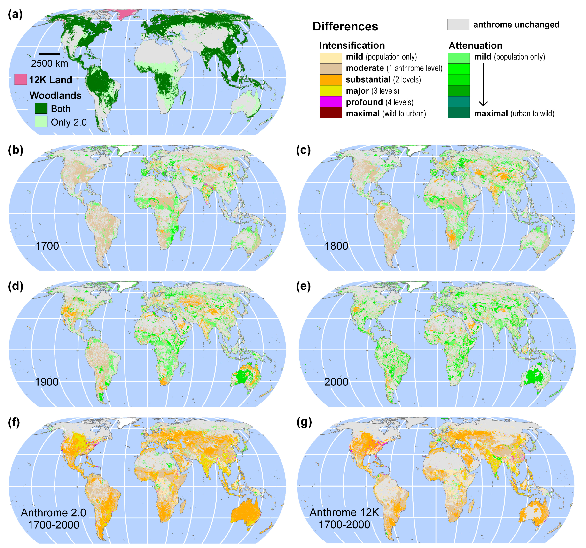
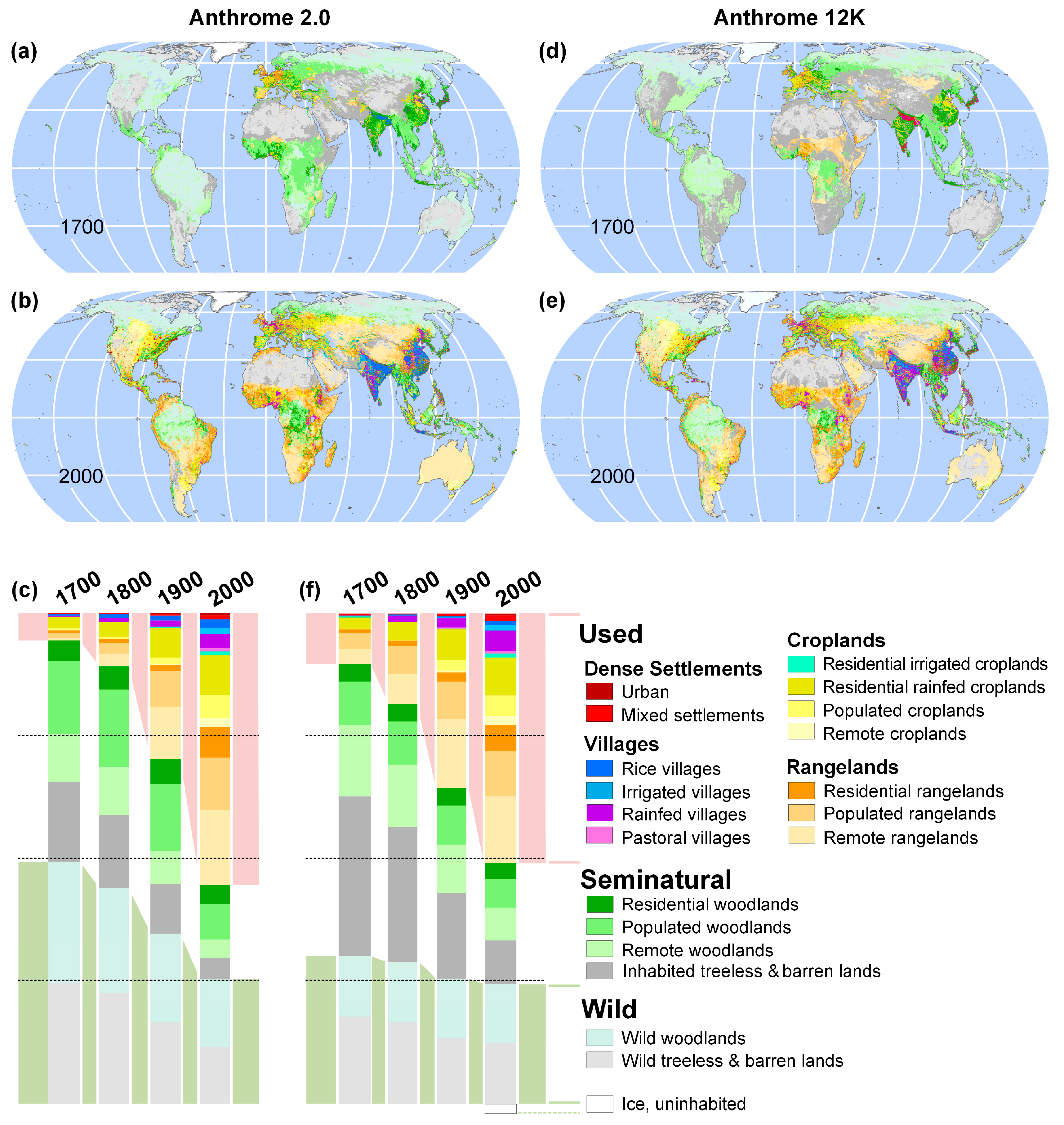
Other major differences between Anthromes 2.0 and Anthromes 12K maps are evident in maps highlighting differences between anthrome maps (Figure 1), in land area computations for 2000 CE (Table 3) versus 1700 CE (Table 4) and in anthrome maps illustrating these two time periods and relative changes in anthrome areas over this interval (Figure 2). In 2000 CE, the largest differences were related to a shift from about 32% of global land area covered by Rangelands in Anthromes 2.0 to about 27% in Anthromes 12K, with most of this reduction in Rangelands caused by their reclassification as Seminatural Inhabited treeless and barren lands, which is especially evident in Australia, but also in other areas around the world (Table 3, Figure 2b,e). A nearly equivalent opposing effect was evident in the 1700 CE comparison, where Rangelands were increased by about 5% of Earth’s global land area in Anthromes 12K over Anthromes 2.0 (Table 4); a change in classification most evident in Sub-Saharan Africa (Figure 2c). The largest difference between Anthromes 12K and Anthromes 2.0 was observed in 1700 CE; a massive reduction in Wildlands, by nearly 17% of Earth’s total land area, caused by a shift largely to Seminatural but also to Rangelands anthromes (Table 4). As a result, the area of Wildlands remaining in 1700 CE was only about 31% in Anthromes 12K, in contrast with more than 49% in Anthromes 2.0; a huge alteration in the trajectory of Earth’s transformation by land use from 1700 to 2000 CE, when Wildlands remain in about 25% of Earth’s land area (Figure 1f,g and Figure 2).
Differences in anthrome maps include widely scattered patches around the world where anthrome classification patterns either intensified or attenuated (Figure 1 and Figure 2). While these were largely explained by changes in rangelands (generally lower in 2000 CE and higher in 1700 CE) versus seminatural lands (generally higher in all time periods), other differences are also evident. One specific area differing substantially between Anthromes 12K and Anthromes 2.0 is the Ganges plain in India and parts of South India in 1700 CE, where mixed settlements and rainfed villages appear in Anthromes 12K and rice villages in Anthromes 2.0. As the main difference between these anthrome classes was the prevalence of irrigated rice cultivation, an error in the HYDE 3.2 rice map for 1700 CE could explain this.
3.2. Anthrome Changes 10,000 BCE to 2015 CE
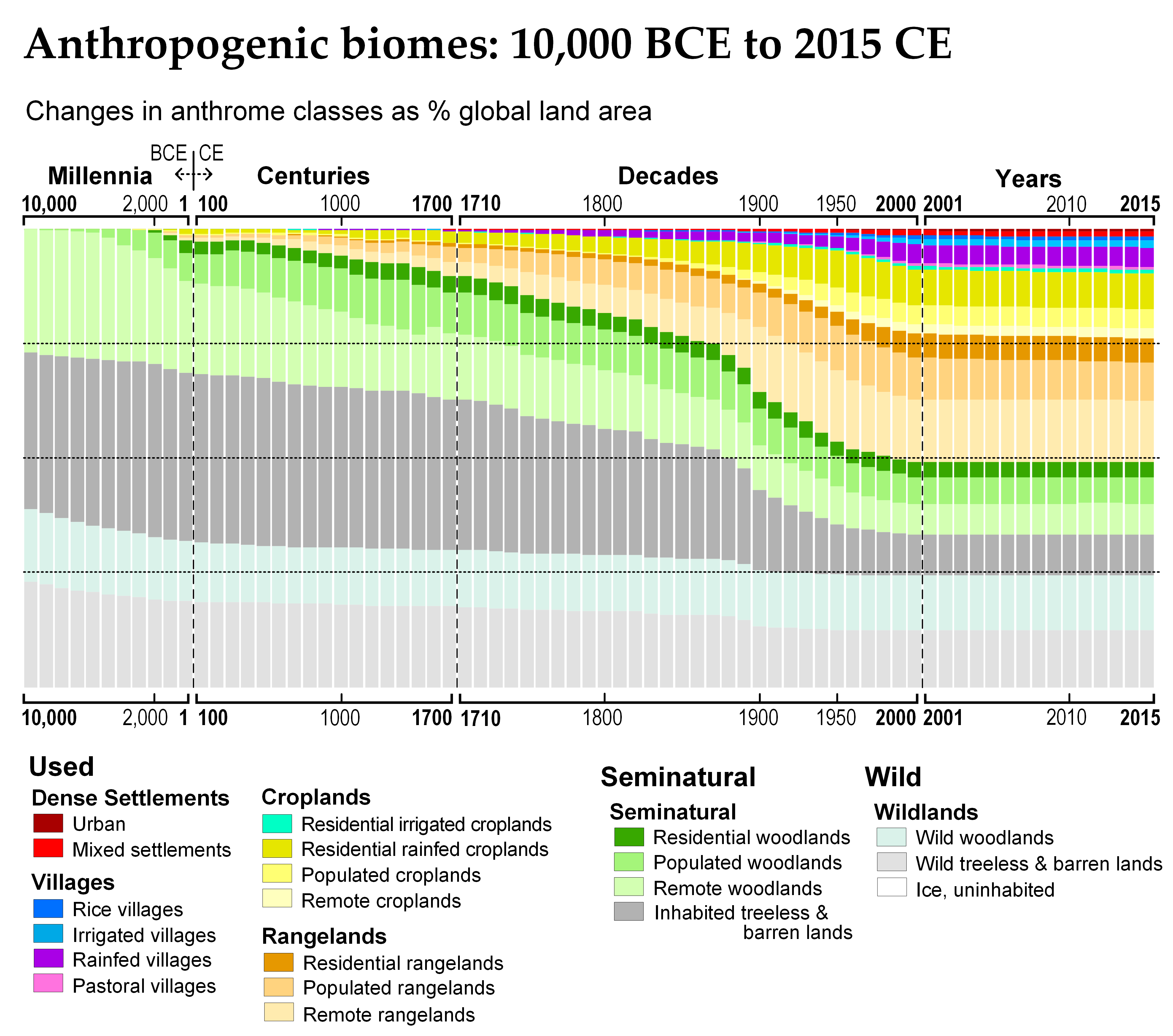
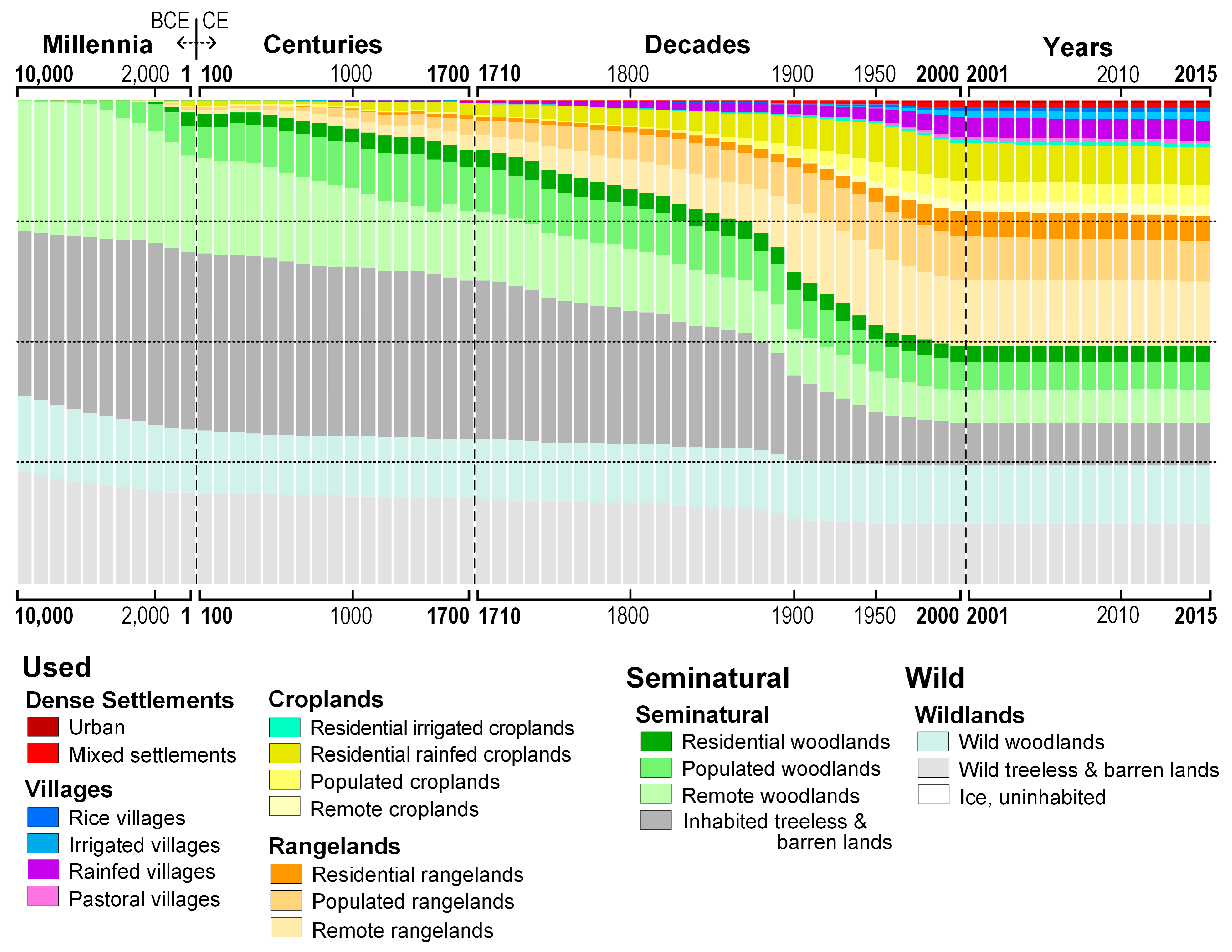
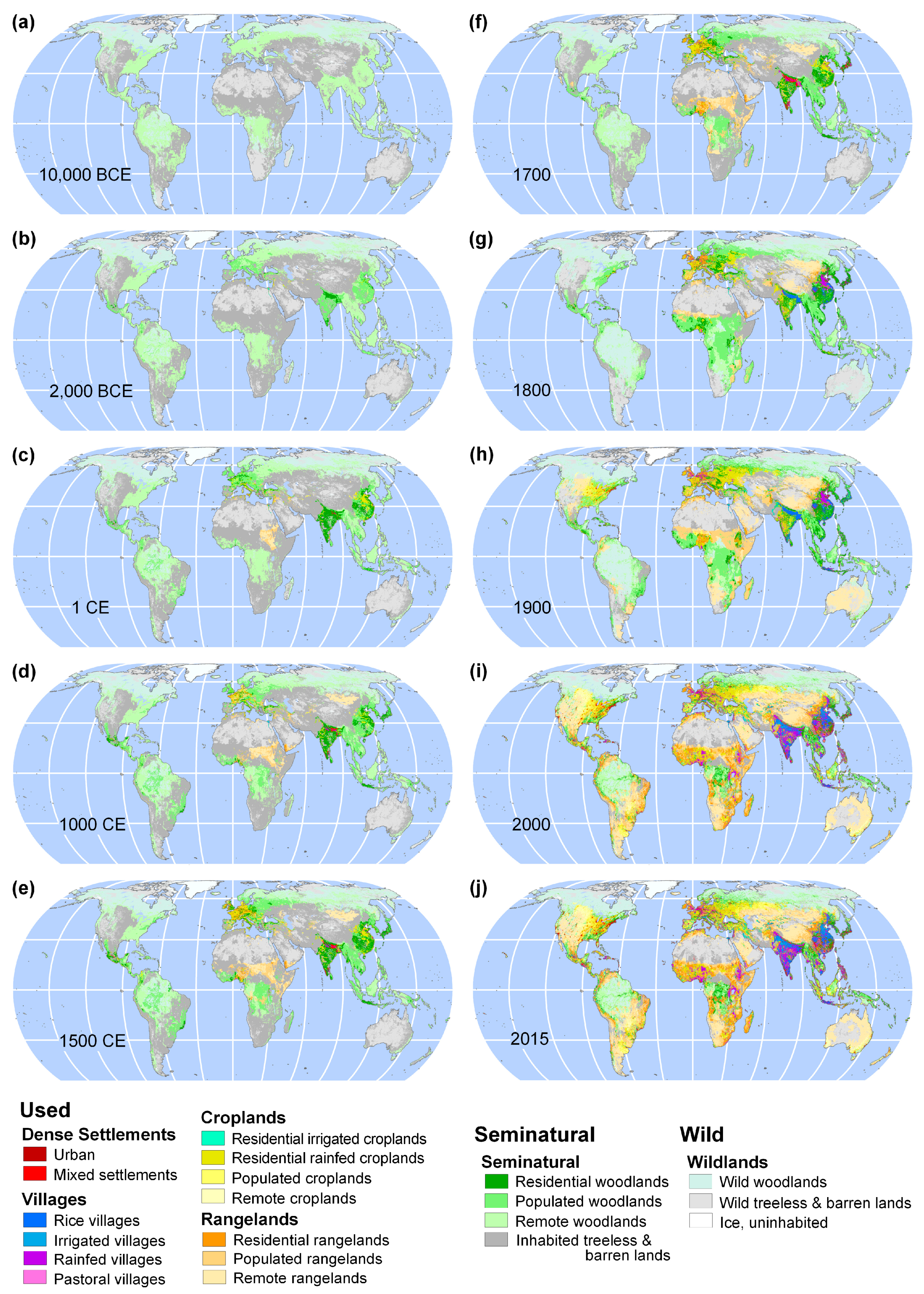
Global changes in anthrome areas from 10,000 BCE to 2015 CE are illustrated in Figure 3 and using anthrome maps for selected time points in Figure 4; anthrome areas for every time point in Anthromes 12K are in Table S1. In 10,000 BCE, Earth’s terrestrial surface consisted entirely of Seminatural (~60%) and Wild (~40%) anthromes. By 2015 CE, Used anthromes covered about half of Earth’s land, with the remainder about equally divided between Seminatural (~24%) and Wild (~26%). In the 12,000 year interval in between, changes in anthromes maps highlight major historical trends in the spread and establishment of agricultural and urban societies around the world that are incorporated into the HYDE 3.2 dataset [35].
The first Dense settlements and Rangelands anthromes appear in 8000 BCE, Croplands anthromes appear in 7,000 BCE, and Village anthromes in 6000 BCE. Yet the global extent of Used anthromes did not reach 1% of Earth’s land area until sometime between 2,000 BCE (0.3%) and 1000 BCE (1.4%). By 1 CE, dense settlements, villages, croplands, and rangelands anthromes are widely present across substantial areas of Mediterranean Europe, The Middle East, Africa, and East Asia (Figure 4).
From their first appearance, Used anthromes have generally increased over time, first covering 5% of Earth’s land between 800 and 900 CE, 10% by 1700 CE, 25% by 1880, and 50% around 2000 CE. This long-term transformation of Wild and Seminatural anthromes into Used anthromes has proceeded fairly steadily over time, though this transformation appears to accelerate in the late 1800s. During this time of accelerating land use, between 1800 and 2000 CE, about 15% of Earth’s remaining Wildlands were converted to Used and Seminatural anthromes, and more than half of Earth’s Seminatural anthromes were transformed into Used anthromes, only slowing down near the end of the 20th century (Figure 3). This accelerated transformation is readily observed in anthrome maps for this interval, with Used anthromes appearing rather suddenly and dramatically across North America by 1900, but also in many other regions around the world (Figure 4g,h,i). In the 15 years from 2000 CE to 2015 CE, the most recent year that Anthromes 12K data are available, anthrome changes were relatively minor, the largest being an approximately 1% decline in Rangeland anthromes.
4. Discussion
4.1. Comparing Anthromes 12K with Anthromes 2.0
In general, Anthromes 12K and Anthromes 2.0 maps were more similar in 2000 CE than in 1700 CE (Table 2, Table 3 and Table 4; Figure 1 and Figure 2). This is likely owing to the use of remote sensing data, rather than model predictions, for land use mapping in recent decades. Still, statistical indicators highlighted significant differences between Anthromes 12K and Anthromes 2.0 maps in every time interval, though these differences were within levels considered acceptable in previous comparisons across anthrome and biome maps in prior published work (Table 2; [24]). Minor changes were introduced through the expansion of anthromes classification to include land covered by permanent ice, but the main cause of differences in anthrome maps was general improvements in the land use data inputs used for anthrome classification, especially those for pastures and rangelands, together with a shift to a new woodland cover dataset.
4.1.1. General Improvements in Land Use and Other Inputs
Overall, the greatest differences between Anthromes 12K and Anthromes 2.0 were evident in periods before 1990 CE, when global land use was mapped using models, not direct measurements from remote sensing, through algorithms allocating land use in relation to estimates of population densities and land use per capita [43]. HYDE 3.2 land use estimates are more accurate than those of HYDE 3.1, whose land use allocation model assumed that past rates of land use per capita were largely unchanged from those of recent times [8,35,43]. For this reason, early land use estimates are generally higher in HYDE 3.2 than in HYDE 3.1, owing to a greater reliance on historical evidence of changes in land use per capita, which tends to be far higher in the past than in current times, because of land use intensification in response to increasing demand from human populations and decreasing land availability per capita [8,43]. The ability to map anthromes over the entire interval from 10,000 BCE to 2015 CE entirely using data inputs from HYDE 3.2 is also a major advance over the long-term, because HYDE 3.2 is not only internally consistent across data layers, the full set of data layers is regularly updated with new and improved historical population and land use data [35], enabling the regular updating of anthrome maps as well.
4.1.2. Pastures and Rangelands
Though Anthromes 2.0 and Anthromes 12K maps were quite similar in 2000 CE, the major exception was the reclassification of most of Central Australia as Wildlands rather than Rangelands (Figure 2b vs. Figure 2e); the result of a major upgrade in the accuracy of pasture and rangeland mapping in the HYDE 3.2 dataset over the HYDE 3.1 data used in Anthromes 2.0 [35]. In 2000 CE, this caused a major global decrease in anthromes classified as Rangelands (by nearly 4% of Earth’s land area) and in the global area of Used anthromes overall (from 55.5% in Anthromes 2.0 to 50% in Anthromes 12K), helping to address longstanding concerns about overestimates of used land areas in the global mapping of anthromes, and of rangelands in particular (Table 4; [44,45]). These same improvements in pasture mapping methodology had the opposite effect in time periods before 2000 CE, producing substantial increases in Rangeland anthromes in earlier centuries (Table 4; Figure 2).
4.1.3. Woodlands
Anthromes 2.0 mapped woodland anthromes based on the potential natural vegetation biome maps of Ramankutty and Foley [16] while Anthromes 12K mapped woodlands using the global biomes dataset of Prentice et al. [38]; part of the HYDE 3.2 data release [35]. Since the global extent of woodland cover in Prentice et al. [38] was substantially lower than in Ramankutty and Foley [16], 55.3 million versus 74.5 million km2, respectively, woodland anthrome areas tended to be lower in Anthromes 12K than in Anthromes 2.0, especially in earlier time periods where most anthromes were classified as Seminatural or Wild (Table 3 and Table 4). This difference in woodland area was largely the result of including Savanna in the woodland cover definition in Anthromes 2.0, which added about 19 million km2; Prentice et al. [38] includes no single savanna class, and vegetation classes that included savanna were not included in the woodland cover definition of Anthromes 12K. As forest and woodland definitions remain open to some interpretation [46], and global woodland cover in Ramankutty and Foley [16] and Prentice et al. [38] were similar when savannas were not included, the switch to a more restricted definition of woodland cover in Anthromes 12K seems merited, and also agrees well with the 57.6 million km2 “forest zone” mapped by Potapov, et al. [47].
4.2. Long-Term Changes in Anthromes
The higher area of early land use in Anthromes 12K versus Anthromes 2.0 represents a paradigm shift in describing Earth’s transformation by land use from 1700 CE to 2000 CE. While both datasets agreed that Wildlands covered about 25% of Earth’s land in 2000 CE, Wildlands in 1700 CE covered only 31% of global land in Anthromes 12K, compared with more than 49% in Anthromes 2.0. In other words, as a result of improvements in the land use area estimates of HYDE 3.2, the Anthromes 12K dataset explains Earth’s transformation through land use from 1700 to 2000 CE almost entirely as a process of land use intensification, involving shifts from Seminatural to Used anthromes, while Anthromes 2.0 characterized these changes as an approximately equal mix of intensification of land use in Seminatural anthromes and Wildland conversion into Used and Seminatural anthromes. As a whole, this appears to be a major improvement in accurately characterizing Earth’s early transformation through land use, when compared with existing evidence [8,12,48]. Nevertheless, there are major uncertainties remaining in regional and global assessments of early land use [48].
A recent study compared the timing of regional onsets of widespread crop production (crops covering >20% of regional area) in HYDE 3.2 with those assessed by archaeologists and found 21 regions, accounting for 22% of global crop area in 2000 CE, where crop production onsets in HYDE 3.2 occurred >1000 years later than archaeological evidence [12]. On the other hand, when archaeological results were compared with the KK10 global historical reconstruction of anthropogenic land cover changes, crop production onsets often occurred earlier than the archaeological evidence [12]. Taken together with previous intercomparisons of historical global land use change reconstructions and their potential global environmental consequences [6,8], it is clear how much work is still needed to develop more accurate and empirically-based global reconstructions of anthropogenic transformation of the biosphere caused by human populations and their use of land from their first beginnings, thousands of years ago [49,50,51].
Whenever substantial improvements in historical reconstructions of land use and population allow anthrome maps to be upgraded, it is hoped that the current Anthromes 12K dataset, version 1.0, will be upgraded as well. Future advances in assessing early use of land, especially by hunter-gatherer societies [12,52,53], will also be critical, and could enable new strategies for anthrome classification and mapping that incorporate land management using fire, the propagation of favored species, and other ecological transformations not currently included explicitly in anthrome classification and mapping.
4.3. Applications of Anthromes 12K
As with prior anthrome datasets [23,24], Anthromes 12K offers many opportunities to investigate the global consequences of long-term changes in the global reshaping of ecology by human societies. One key investigation yet to be completed using these new data is an assessment of the global transformation of terrestrial biomes over the past 12,000 years, potentially using similar statistical techniques as those used in prior assessments based on earlier datasets [6,24]. The many other assessments of Earth’s ecological and social patterns, processes, and dynamics that have utilized prior anthrome datasets are also clear targets for new and improved investigations using Anthromes 12K, including, for example, studies of biogeography and biodiversity [30,54,55,56], primary productivity [57], fire [58] conservation [29,59,60,61,62], disease [63], and ecological research itself [64]. The freely downloadable and newly updated time series of anthropogenic global changes represented in the Anthromes 12K dataset (https://0-doi-org.brum.beds.ac.uk/10.7910/DVN/G0QDNQ) should provide ample resources for researchers aiming to investigate these changes using both new and existing analytical strategies.
5. Conclusions
Anthromes 12K is the first dataset to characterize anthrome changes across Earth’s land over the past 12,000 years. Though it differs in multiple ways from prior anthromes maps, these differences are largely the result of improvements in the data inputs provided by the HYDE 3.2 dataset over those used in prior anthrome reconstructions, especially for pasture and rangelands, together with the inclusion of permanent ice cover in anthromes maps. Another difference, which reduced areas mapped as woodlands, especially in earlier time periods, was caused by use of a different woodland cover map, provided as part of the HYDE 3.2 dataset. This difference, though significant, performed entirely as expected and represented only a change in vegetation cover interpretation within the bounds of existing published estimates rather than a change in data quality.
Anthromes 12K presents a very different narrative of Earth’s transformation by land use than earlier anthrome maps, which represented the terrestrial biosphere, even in 1700 CE, as largely uninhabited and wild, rather than inhabited and seminatural. In Anthromes 12K, this error is corrected, and Earth’s transformation through land use in prehistoric, preindustrial and more recent times is characterized not as an increasingly large-scale conversion of uninhabited wildlands, but rather as an increasingly intensive use of Seminatural and Used anthromes.
As with all global land use history reconstructions, Anthromes 12K is no more accurate or reliable than the evidence and models used to produce them. The HYDE 3.2 dataset used to produce Anthromes 12K, while certainly a major improvement over HYDE 3.1, which was used to produce Anthromes 2.0, is already known to include substantial discrepancies from existing archaeological and historical knowledge. Specifically, in many regions, intensive agriculture appears later by centuries to millennia in HYDE 3.2 when compared to a recent global reconstruction by archaeologists [12]. For this reason, like HYDE and other historical reconstructions, Anthromes 12K should be considered a work in progress, to be updated when improved input data become available. Nevertheless, Anthromes 12K represents a major improvement over all prior anthrome datasets, setting the standard for future efforts to characterize and understand Earth’s transformation by human societies and their use of land.
Supplementary Materials
The following are available online at https://0-www-mdpi-com.brum.beds.ac.uk/2073-445X/9/5/129/s1, Table S1: Anthromes 12K Land Areas.
Author Contributions
E.C.E., K.K.G., and A.H.W.B. conceived and wrote the paper, conducted analyses and prepared figures. All authors have read and agreed to the published version of the manuscript.
Funding
Ellis contributions were supported in part by US NSF grant CNS 1125210. Klein Goldewijk contributions were supported by NWO VENI grant no. 016.158.021.
Acknowledgments
This is a contribution from the Global Land Programme of Future Earth (http://glp.earth). This study was also undertaken as part of the Past Global Changes (PAGES) LandCover6K working group project, which in turn received support from the US National Science Foundation and the Swiss Academy of Sciences.
Conflicts of Interest
The authors declare no conflict of interest.
Appendix A
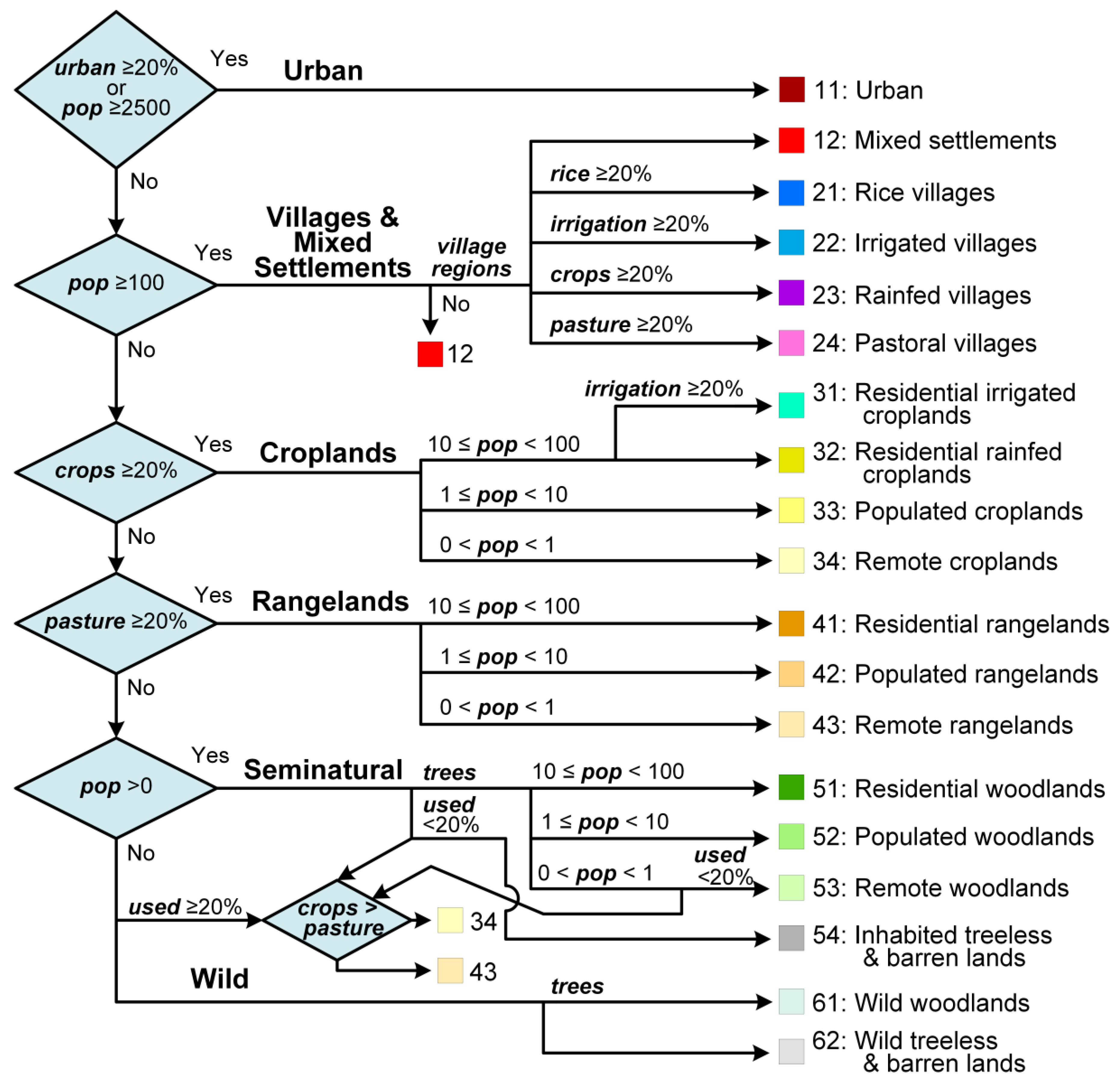
Anthromes v2.0 classification flowchart. Five anthrome levels are labeled in large bold text near the left and anthrome classes and symbols (color coded boxes) at far right. Data inputs to the model are in italics: urban = % urban land cover, pop = population density (persons km−2), rice = % cover by rice, irrigation = % land area irrigated, crops = % area covered by crops, pasture = % area covered by pastures, used = urban + crops + pasture, trees = areas potentially covered by trees, based on woodlands and savanna potential vegetation cover in [16], village regions = regions with a history of agricultural village development (cells outside North America, Australia and New Zealand). Based on Appendix S3: Anthrome Classification Algorithm, in [24].
Figure A1.
Anthromes v2.0 classification flowchart.

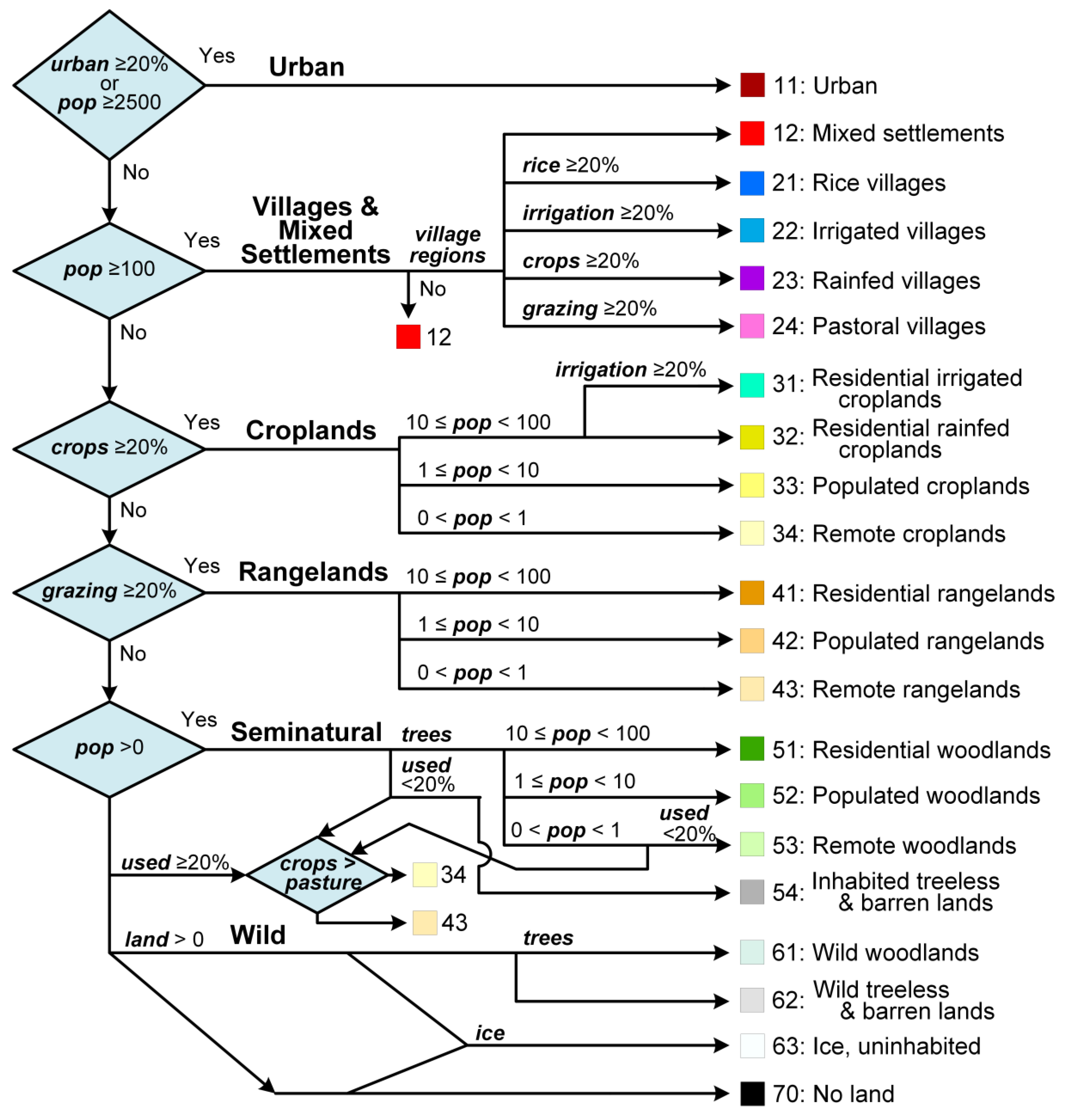
Anthromes v2.1 classification flowchart. Same as Anthromes 2.0, with five changes. First, the grazing variable is substituted for the HYDE 3.1 pasture variable, because HYDE 3.2 now separates the HYDE 3.1 pasture variable into separate pasture = % area covered by intensively managed pastures) and rangeland = extensively managed grazing areas; grazing = pasture + rangeland. Second, land variable classifies cells with land area > 0 (anthromes v2.0 did not include cells without land). Third, trees = areas potentially covered by trees, is based on the 8 forest and woodland biomes in Prentice et al. [38]. Fourth, a new anthrome class = 63 = ice, uninhabited is added; anthromes 2.0 included only ice-free land. Fifth, a no data anthrome class is added = 70 (used only as a placeholder for no data values after classification).
Figure A2.
Anthromes v2.1 classification flowchart.

References
- Newbold, T.; Hudson, L.N.; Hill, S.L.L.; Contu, S.; Lysenko, I.; Senior, R.A.; Borger, L.; Bennett, D.J.; Choimes, A.; Collen, B.; et al. Global effects of land use on local terrestrial biodiversity. Nature 2015, 520, 45–50. [Google Scholar] [CrossRef] [PubMed] [Green Version]
- Foley, J.A.; DeFries, R.; Asner, G.P.; Barford, C.; Bonan, G.; Carpenter, S.R.; Chapin, F.S.; Coe, M.T.; Daily, G.C.; Gibbs, H.K.; et al. Global consequences of land use. Science 2005, 309, 570–574. [Google Scholar] [CrossRef] [PubMed] [Green Version]
- Steffen, W.; Broadgate, W.; Deutsch, L.; Gaffney, O.; Ludwig, C. The trajectory of the anthropocene: The great acceleration. Anthr. Rev. 2015, 2, 81–98. [Google Scholar] [CrossRef]
- Lewis, S.L.; Maslin, M.A. Defining the anthropocene. Nature 2015, 519, 171–180. [Google Scholar] [CrossRef] [PubMed]
- Hurtt, G.; Chini, L.; Frolking, S.; Betts, R.; Feddema, J.; Fischer, G.; Fisk, J.; Hibbard, K.; Houghton, R.; Janetos, A.; et al. Harmonization of land-use scenarios for the period 1500–2100: 600 years of global gridded annual land-use transitions, wood harvest, and resulting secondary lands. Clim. Chang. 2011, 109, 117–161. [Google Scholar] [CrossRef] [Green Version]
- Ellis, E.C. Anthropogenic transformation of the terrestrial biosphere. Proc. R. Soc. A: Math. Phys. Eng. Sci. 2011, 369, 1010–1035. [Google Scholar] [CrossRef]
- Waters, C.N.; Zalasiewicz, J.; Summerhayes, C.; Barnosky, A.D.; Poirier, C.; Gałuszka, A.; Cearreta, A.; Edgeworth, M.; Ellis, E.C.; Ellis, M.; et al. The anthropocene is functionally and stratigraphically distinct from the holocene. Science 2016, 351, aad2622. [Google Scholar] [CrossRef]
- Ellis, E.C.; Kaplan, J.O.; Fuller, D.Q.; Vavrus, S.; Klein Goldewijk, K.; Verburg, P.H. Used planet: A global history. Proc. Natl. Acad. Sci. USA 2013, 110, 7978–7985. [Google Scholar] [CrossRef] [Green Version]
- Ellis, E.C. Ecology in an anthropogenic biosphere. Ecol. Monogr. 2015, 85, 287–331. [Google Scholar] [CrossRef]
- Smith, B.D.; Zeder, M.A. The onset of the anthropocene. Anthropocene 2013, 4, 8–13. [Google Scholar] [CrossRef]
- Kirch, P.V. Archaeology and global change: The holocene record. Annu. Rev. Environ. Resour. 2005, 30, 409. [Google Scholar] [CrossRef]
- Stephens, L.; Fuller, D.; Boivin, N.; Rick, T.; Gauthier, N.; Kay, A.; Marwick, B.; Geralda, C.; Armstrong, D.; Barton, C.M.; et al. Archaeological assessment reveals earth’s early transformation through land use. Science 2019, 365, 897–902. [Google Scholar] [CrossRef] [PubMed] [Green Version]
- Doughty, C.E. Preindustrial human impacts on global and regional environment. Annu. Rev. Environ. Resour. 2013, 38, 503–527. [Google Scholar] [CrossRef]
- Ruddiman, W.F.; Fuller, D.Q.; Kutzbach, J.E.; Tzedakis, P.C.; Kaplan, J.O.; Ellis, E.C.; Vavrus, S.J.; Roberts, C.N.; Fyfe, R.; He, F.; et al. Late holocene climate: Natural or anthropogenic? Rev. Geophys. 2016, 54, 93–118. [Google Scholar] [CrossRef] [Green Version]
- Kaplan, J.O.; Krumhardt, K.M.; Ellis, E.C.; Ruddiman, W.F.; Lemmen, C.; Klein Goldewijk, K. Holocene carbon emissions as a result of anthropogenic land cover change. Holocene 2011, 21, 775–791. [Google Scholar] [CrossRef] [Green Version]
- Ramankutty, N.; Foley, J.A. Estimating historical changes in global land cover: Croplands from 1700 to 1992. Glob. Biogeochem. Cycles 1999, 13, 997–1027. [Google Scholar] [CrossRef]
- Klein Goldewijk, K.; Beusen, A.; van Drecht, G.; de Vos, M. The hyde 3.1 spatially explicit database of human induced global land use change over the past 12,000 years. Glob. Ecol. Biogeogr. 2011, 20, 73–86. [Google Scholar] [CrossRef]
- Klein Goldewijk, K.; Beusen, A.; Janssen, P. Long-term dynamic modeling of global population and built-up area in a spatially explicit way: Hyde 3.1. Holocene 2010, 20, 565–573. [Google Scholar] [CrossRef] [Green Version]
- Klein Goldewijk, K. Estimating global land use change over the past 300 years: The hyde database. Glob. Biogeochem. Cycles 2001, 15, 417–433. [Google Scholar] [CrossRef]
- Pongratz, J.; Reick, C.; Raddatz, T.; Claussen, M. A reconstruction of global agricultural areas and land cover for the last millennium. Glob. Biogeochem. Cycles 2008, 22, GB3018. [Google Scholar] [CrossRef]
- Olofsson, J.; Hickler, T. Effects of human land-use on the global carbon cycle during the last 6,000 years. Veg. Hist. Archaeobotany 2008, 17, 605–615. [Google Scholar] [CrossRef] [Green Version]
- Sanderson, E.W.; Jaiteh, M.; Levy, M.A.; Redford, K.H.; Wannebo, A.V.; Woolmer, G. The human footprint and the last of the wild. Bioscience 2002, 52, 891–904. [Google Scholar] [CrossRef]
- Ellis, E.C.; Ramankutty, N. Putting people in the map: Anthropogenic biomes of the world. Front. Ecol. Environ. 2008, 6, 439–447. [Google Scholar] [CrossRef] [Green Version]
- Ellis, E.C.; Klein Goldewijk, K.; Siebert, S.; Lightman, D.; Ramankutty, N. Anthropogenic transformation of the biomes, 1700 to 2000. Glob. Ecol. Biogeogr. 2010, 19, 589–606. [Google Scholar] [CrossRef]
- National Geographic Society. National Geographic Atlas of the World, 10th ed.; National Geographic Society: Washington, DC, USA, 2014; p. 448. [Google Scholar]
- Freeman, S.; Quillin, K.; Allison, L.; Black, M.; Podgorski, G.; Taylor, E.; Carmichael, J. Biological Science, 6th ed.; Benjamin-Cummings Publishing Company: San Francisco, CA, USA, 2016; p. 1360. [Google Scholar]
- Smith, J.A.; Powell, L.A.; Brown, M.B. Training wildlife biologists for work in anthromes. In Reference Module in Earth Systems and Environmental Sciences; Elsevier: Amsterdam, The Netherlands, 2019. [Google Scholar]
- Dinerstein, E.; Olson, D.; Joshi, A.; Vynne, C.; Burgess, N.D.; Wikramanayake, E.; Hahn, N.; Palminteri, S.; Hedao, P.; Noss, R.; et al. An ecoregion-based approach to protecting half the terrestrial realm. Bioscience 2017, 67, 534–545. [Google Scholar] [CrossRef]
- Martin, L.J.; Quinn, J.E.; Ellis, E.C.; Shaw, M.R.; Dorning, M.A.; Hallett, L.M.; Heller, N.E.; Hobbs, R.J.; Kraft, C.E.; Law, E.; et al. Biodiversity conservation opportunities across the world’s anthromes. Divers. Distrib. 2014, 20, 745–755. [Google Scholar] [CrossRef] [Green Version]
- Miraldo, A.; Li, S.; Borregaard, M.K.; Flórez-Rodríguez, A.; Gopalakrishnan, S.; Rizvanovic, M.; Wang, Z.; Rahbek, C.; Marske, K.A.; Nogués-Bravo, D. An anthropocene map of genetic diversity. Science 2016, 353, 1532–1535. [Google Scholar] [CrossRef]
- Chapin, F.S., III; Matson, P.A.; Vitousek, P.M. Principles of Terrestrial Ecosystem Ecology, 2nd ed.; Springer: Berlin, Germany, 2012. [Google Scholar]
- Merritts, D.; Menking, K.; DeWet, A. Environmental Geology: An Earth Systems Approach, 2nd ed.; W. H. Freeman: New York, NY, USA, 2014; p. 604. [Google Scholar]
- He, F.; Vavrus, S.J.; Kutzbach, J.E.; Ruddiman, W.F.; Kaplan, J.O.; Krumhardt, K.M. Simulating global and local surface temperature changes due to holocene anthropogenic land cover change. Geophys. Res. Lett. 2014, 41, 623–631. [Google Scholar] [CrossRef]
- Lawrence, D.M.; Hurtt, G.C.; Arneth, A.; Brovkin, V.; Calvin, K.V.; Jones, A.D.; Jones, C.D.; Lawrence, P.J.; de Noblet-Ducoudré, N.; Pongratz, J.; et al. The land use model intercomparison project (lumip) contribution to cmip6: Rationale and experimental design. Geosci. Model Dev. 2016, 9, 2973–2998. [Google Scholar] [CrossRef] [Green Version]
- Klein Goldewijk, K.; Beusen, A.; Doelman, J.; Stehfest, E. Anthropogenic land use estimates for the holocene—hyde 3.2. Earth Syst. Sci. Data 2017, 9, 927–953. [Google Scholar] [CrossRef] [Green Version]
- Siebert, S.; Doll, P.; Feick, S.; Hoogeveen, J.; Frenken, K. Global Map of Irrigation Areas Version 4.0.1; Johann Wolfgang Goethe University: Frankfurt am Main, Germany, 2007. [Google Scholar]
- Monfreda, C.; Ramankutty, N.; Foley, J.A. Farming the planet: 2. Geographic distribution of crop areas, yields, physiological types, and net primary production in the year 2000. Glob. Biogeochem. Cycles 2008, 22, GB1022. [Google Scholar] [CrossRef]
- Prentice, I.C.; Cramer, W.; Harrison, S.P.; Leemans, R.; Monserud, R.A.; Solomon, A.M. A global biome model based on plant physiology and dominance, soil properties and climate. J. Biogeogr. 1992, 19, 117–134. [Google Scholar] [CrossRef]
- Visser, H.; de Nijs, T. The map comparison kit. Environ. Model. Softw. 2006, 21, 346–358. [Google Scholar] [CrossRef]
- Rees, W.G. Comparing the spatial content of thematic maps. Int. J. Remote Sens. 2008, 29, 3833–3844. [Google Scholar] [CrossRef]
- Rea, L.M.; Parker, R.A. Designing and Conducting Survey Research: A Comprehensive Guide; Jossey-Bass: San Francisco, CA, USA, 1997. [Google Scholar]
- Olson, D.M.; Dinerstein, E.; Wikramanayake, E.D.; Burgess, N.D.; Powell, G.V.N.; Underwood, E.C.; D’Amico, J.A.; Itoua, I.; Strand, H.E.; Morrison, J.C.; et al. Terrestrial ecoregions of the world: A new map of life on earth. Bioscience 2001, 51, 933–938. [Google Scholar] [CrossRef]
- Klein Goldewijk, K.; Dekker, S.C.; van Zanden, J.L. Per-capita estimations of long-term historical land use and the consequences for global change research. J. Land Use Sci. 2017, 12, 313–337. [Google Scholar] [CrossRef] [Green Version]
- Phelps, L.N.; Kaplan, J.O. Land use for animal production in global change studies: Defining and characterizing a framework. Glob. Chang. Biol. 2017, 23, 4457–4471. [Google Scholar] [CrossRef] [Green Version]
- Sayre, N.F.; Davis, D.K.; Bestelmeyer, B.; Williamson, J.C. Rangelands: Where anthromes meet their limits. Land 2017, 6, 31. [Google Scholar] [CrossRef] [Green Version]
- Chazdon, R.L.; Brancalion, P.H.S.; Laestadius, L.; Bennett-Curry, A.; Buckingham, K.; Kumar, C.; Moll-Rocek, J.; Vieira, I.C.G.; Wilson, S.J. When is a forest a forest? Forest concepts and definitions in the era of forest and landscape restoration. Ambio 2016, 45, 538–550. [Google Scholar] [CrossRef]
- Potapov, P.; Hansen, M.C.; Laestadius, L.; Turubanova, S.; Yaroshenko, A.; Thies, C.; Smith, W.; Zhuravleva, I.; Komarova, A.; Minnemeyer, S.; et al. The last frontiers of wilderness: Tracking loss of intact forest landscapes from 2000 to 2013. Sci. Adv. 2017, 3, e1600821. [Google Scholar] [CrossRef] [Green Version]
- Roberts, N. How humans changed the face of earth. Science 2019, 365, 865–866. [Google Scholar] [CrossRef] [PubMed]
- Klein Goldewijk, K.; Verburg, P.H. Uncertainties in global-scale reconstructions of historical land use: An illustration using the hyde data set. Landsc. Ecol. 2013, 28, 861–877. [Google Scholar] [CrossRef]
- Harrison, S.P.; Gaillard, M.J.; Stocker, B.D.; Vander Linden, M.; Klein Goldewijk, K.; Boles, O.; Braconnot, P.; Dawson, A.; Fluet-Chouinard, E.; Kaplan, J.O.; et al. Development and testing scenarios for implementing land use and land cover changes during the holocene in earth system model experiments. Geosci. Model Dev. 2020, 13, 805–824. [Google Scholar] [CrossRef] [Green Version]
- Gaillard, M.-J.; Morrison, K.D.; Madella, M.; Whitehouse, N. Past land-use and land-cover change: The challenge of quantification at the subcontinental to global scales. Pages Mag. 2018, 26, 3. [Google Scholar] [CrossRef] [Green Version]
- Smith, B.D. General patterns of niche construction and the management of ‘wild’ plant and animal resources by small-scale pre-industrial societies. Philos. Trans. R. Soc. B Biol. Sci. 2011, 366, 836–848. [Google Scholar] [CrossRef] [Green Version]
- Bliege Bird, R.; Nimmo, D. Restore the lost ecological functions of people. Nat. Ecol. Evol. 2018, 2, 1050–1052. [Google Scholar] [CrossRef]
- Pekin, B.K.; Pijanowski, B.C. Global land use intensity and the endangerment status of mammal species. Divers. Distrib. 2012, 18, 909–918. [Google Scholar] [CrossRef]
- Ellis, E.C.; Antill, E.C.; Kreft, H. All is not loss: Plant biodiversity in the anthropocene. PLoS ONE 2012, 7, e30535. [Google Scholar] [CrossRef] [Green Version]
- Rowan, J.; Beaudrot, L.; Franklin, J.; Reed, K.E.; Smail, I.E.; Zamora, A.; Kamilar, J.M. Geographically divergent evolutionary and ecological legacies shape mammal biodiversity in the global tropics and subtropics. Proc. Natl. Acad. Sci. USA 2020, 117, 1559–1565. [Google Scholar] [CrossRef]
- Mueller, T.; Dressler, G.; Tucker, C.; Pinzon, J.; Leimgruber, P.; Dubayah, R.; Hurtt, G.; Böhning-Gaese, K.; Fagan, W. Human land-use practices lead to global long-term increases in photosynthetic capacity. Remote Sens. 2014, 6, 5717. [Google Scholar] [CrossRef] [Green Version]
- Pereira, J.M.C.; Turkman, M.A.A.; Turkman, K.F.; Oom, D. Anthromes displaying evidence of weekly cycles in active fire data cover 70% of the global land surface. Sci. Rep. 2019, 9, 11424. [Google Scholar] [CrossRef] [PubMed]
- Ibisch, P.L.; Hoffmann, M.T.; Kreft, S.; Pe’er, G.; Kati, V.; Biber-Freudenberger, L.; DellaSala, D.A.; Vale, M.M.; Hobson, P.R.; Selva, N. A global map of roadless areas and their conservation status. Science 2016, 354, 1423–1427. [Google Scholar] [CrossRef]
- Garnett, S.; Fernández-Llamazares, Á.; Robinson, C.; Ellis, E.C.; Geyle, H.; Leiper, I.; Watson, J.; Fa, J.E.; Zander, K.; Jackson, M.V.; et al. Indigenous peoples are crucial for conservation—A quarter of all land is in their hands. The Conversation, 2018 17 July. [Google Scholar]
- Jacobson, A.P.; Riggio, J.; Tait, A.M.; Baillie, J.E. Global areas of low human impact (‘low impact areas’) and fragmentation of the natural world. Sci. Rep. 2019, 9, 14179. [Google Scholar] [CrossRef] [PubMed]
- Gibson, D.; Quinn, J. Application of anthromes to frame scenario planning for landscape-scale conservation decision making. Land 2017, 6, 33. [Google Scholar] [CrossRef] [Green Version]
- Brearley, G.; Rhodes, J.; Bradley, A.; Baxter, G.; Seabrook, L.; Lunney, D.; Liu, Y.; McAlpine, C. Wildlife disease prevalence in human-modified landscapes. Biol. Rev. 2013, 88, 427–442. [Google Scholar] [CrossRef] [PubMed]
- Martin, L.J.; Blossey, B.; Ellis, E. Mapping where ecologists work: Biases in the global distribution of terrestrial ecological observations. Front. Ecol. Environ. 2012, 10, 195–201. [Google Scholar] [CrossRef] [Green Version]
Figure 1.
Differences between Anthromes 12K and Anthromes 2.0 maps. (a) Differences in land mask (“12K Land”) and woodland cover, illustrating overlap between woodland cover maps (“Both”), and areas with woodland cover only in Anthromes 2.0 (“2.0”). Differences in years (b) 1700, (c) 1800, (d) 1900 and (e) 2000 CE. Differences are highlighted in terms of relative intensification or attenuation of anthrome use class in Anthromes 12K. Intensification indicates shifts in anthrome level towards dense settlements and away from wildlands and shifts within anthrome levels (“mild”) towards higher land use intensity (irrigation) and/or population density. Attenuation highlights shifts in the opposite direction, towards less intensive use and less dense populations within anthromes. Long-term changes between 1700 and 2000 CE in (f) Anthromes 2.0 and (g) Anthromes 12K are highlighted using the same legend. Eckert IV projection.

Figure 2.
Comparison of Anthromes 2.0 and Anthromes 12K maps for 1700 and 2000 CE, and global area changes from 1700 to 2000 CE. Anthromes 2.0 maps for (a) 1700 and (b) 2000 and (c) changes in global land areas as percent ice-free land (stacked bars). Anthromes 12K maps for (d) 1700 and (e) 2000 and (f) changes in global land areas as percent ice-free land (stacked bars). Relative area of Ice, uninhabited is indicated for 2000 CE; this did not change significantly over time. Maps in Eckert IV projection.

Figure 3.
Changes in anthrome areas from 10,000 BCE to 2015 CE for all time intervals in the Anthromes 12K dataset. Relative global areas are indicated using stacked bars, which add up to the total global land area, not including Ice, uninhabited, which showed no significant changes over time.
Figure 3.
Changes in anthrome areas from 10,000 BCE to 2015 CE for all time intervals in the Anthromes 12K dataset. Relative global areas are indicated using stacked bars, which add up to the total global land area, not including Ice, uninhabited, which showed no significant changes over time.

Figure 4.
Anthromes 12K maps for selected times; (a) 10,000 BCE, (b) 2,000 BCE, (c) 1 CE, (d) 1000 CE, (e) 1500 CE, (f) 1700 CE, (g) 1800 CE, (h) 1900 CE, (i) 2000 CE, (j) 2015 CE. Eckert IV projection.
Figure 4.
Anthromes 12K maps for selected times; (a) 10,000 BCE, (b) 2,000 BCE, (c) 1 CE, (d) 1000 CE, (e) 1500 CE, (f) 1700 CE, (g) 1800 CE, (h) 1900 CE, (i) 2000 CE, (j) 2015 CE. Eckert IV projection.


Table 1.
Anthromes 2.1 classification, including six anthrome levels, including Wildlands and 20 anthromes classes (Appendix A).
Table 1.
Anthromes 2.1 classification, including six anthrome levels, including Wildlands and 20 anthromes classes (Appendix A).
| Code | Name | Description |
|---|---|---|
| Dense settlements: Urban and other nonagricultural dense settlements | ||
| 11 | Urban | Densely built-up environments with very high populations |
| 12 | Mixed settlements | Suburbs, towns and rural settlements with high but fragmented populations |
| Villages: Densely populated agricultural settlements | ||
| 21 | Rice villages | Villages characterized by paddy rice |
| 22 | Irrigated villages | Villages characterized by irrigated crops |
| 23 | Rainfed villages | Villages characterized by rainfed agriculture |
| 24 | Pastoral villages | Villages characterized by pasture and rangeland |
| Croplands: Lands used mainly for annual crops | ||
| 31 | Residential irrigated croplands | Irrigated croplands with substantial human populations |
| 32 | Residential rainfed croplands | Rainfed croplands with substantial human populations |
| 33 | Populated rainfed croplands | Croplands with significant human populations |
| 34 | Remote croplands | Croplands without significant populations (irrigated and rainfed) |
| Rangelands: Lands used for pasture and livestock grazing | ||
| 41 | Residential rangelands | Rangelands with substantial human populations |
| 42 | Populated rangelands | Rangelands with significant human populations |
| 43 | Remote rangelands | Rangelands without significant human populations |
| Seminatural lands: Inhabited lands with minor use for permanent agriculture and settlements | ||
| 51 | Residential woodlands | Forest biome regions with minor land use and substantial populations |
| 52 | Populated woodlands | Forest biome regions with minor land use and significant populations |
| 53 | Remote woodlands | Forest biome regions with minor land use without significant populations |
| 54 | Inhabited treeless and barren lands | Regions without natural tree cover having only minor land use and a range of populations |
| Wildlands: Lands without human populations or substantial land use | ||
| 61 | Wild woodlands | Forests |
| 62 | Wild treeless and barren lands | Regions without natural tree cover (grasslands, shrublands, tundra, desert and barren lands) |
| 63 | Ice, uninhabited | Regions covered by permanent ice |
Table 2.
Statistical indicators of agreement between Anthromes 12K and Anthromes 2.0 maps.
| Statistic | 1700 CE | 1800 CE | 1900 CE | 2000 CE |
|---|---|---|---|---|
| K | 0.519 | 0.516 | 0.518 | 0.573 |
| Klocation | 0.758 | 0.720 | 0.661 | 0.685 |
| Khistogram | 0.685 | 0.717 | 0.783 | 0.837 |
| Cramer’s V | 0.437 | 0.435 | 0.481 | 0.579 |
Table 3.
Comparison of 2000 CE anthrome levels (bold text) and classes in Anthromes 12K and Anthromes 2.0. Global land areas in km2, with percent global land area in parentheses. Difference computed by subtracting Anthromes 2.0 from Anthromes 12K.
Table 3.
Comparison of 2000 CE anthrome levels (bold text) and classes in Anthromes 12K and Anthromes 2.0. Global land areas in km2, with percent global land area in parentheses. Difference computed by subtracting Anthromes 2.0 from Anthromes 12K.
| Anthrome Level/Class | Anthromes 2.0 | Anthromes 12K | Difference |
|---|---|---|---|
| Dense settlements | 1,599,504 (1.25) | 1,944,387 (1.48) | 344,883 (0.26) |
| 11: Urban | 684,360 (0.53) | 571,287 (0.43) | 113,073 (−0.09) |
| 12: Mixed settlements | 915,144 (0.71) | 1,373,100 (1.04) | 457,956 (0.35) |
| Villages | 8,324,877 (6.49) | 8,573,609 (6.5) | 248,732 (0.19) |
| 21: Rice villages | 2,195,127 (1.71) | 926,154 (0.70) | −1,268,973 (−0.96) |
| 22: Irrigated villages | 1,733,295 (1.35) | 1,589,109 (1.21) | −144,186 (−0.11) |
| 23: Rainfed villages | 3,576,908 (2.79) | 5,331,507 (4.05) | 1,754,599 (1.33) |
| 24: Pastoral villages | 819,547 (0.64) | 726,839 (0.55) | −92,708 (−0.07) |
| Croplands | 19,950,484 (15.56) | 19,065,343 (14.46) | −885,141 (−0.67) |
| 31: Residential irrigated croplands | 1,090,155 (0.85) | 920,859 (0.70) | −169,296 (−0.13) |
| 32: Residential rainfed croplands | 10,307,863 (8.04) | 10,196,049 (7.74) | −111,814 (−0.08) |
| 33: Populated croplands | 6,037,937 (4.71) | 5,308,253 (4.03) | −729,684 (−0.55) |
| 34: Remote croplands | 2,514,529 (1.96) | 2,640,182 (2.00) | 125,653 (0.10) |
| Rangelands | 41,258,202 (32.19) | 36,224,142 (27.48) | −5,034,060 (−3.82) |
| 41: Residential rangelands | 7,908,903 (6.17) | 6,750,195 (5.12) | −1,158,708 (−0.88) |
| 42: Populated rangelands | 13,753,742 (10.73) | 11,747,394 (8.91) | −2,006,348 (−1.52) |
| 43: Remote rangelands | 19,595,557 (15.29) | 17,726,553 (13.45) | −1,869,004 (−1.42) |
| Seminatural | 24,673,582 (19.25) | 32,002,717 (24.28) | 7,329,135 (5.56) |
| 51: Residential woodlands | 4,896,997 (3.82) | 4,198,045 (3.19) | −698,952 (−0.53) |
| 52: Populated woodlands | 9,305,111 (7.26) | 7,673,846 (5.82) | −1,631,265 (−1.24) |
| 53: Remote woodlands | 5,008,400 (3.91) | 8,651,823 (6.56) | 3,643,423 (2.76) |
| 54: Inhabited treeless & barren lands | 5,463,074 (4.26) | 11,479,003 (8.71) | 6,015,929 (4.56) |
| Wildlands | 32,378,963 (25.26) | 33,993,839 (25.79) | 1,614,876 (1.23) |
| 61: Wild woodlands | 17,749,664 (13.85) | 15,463,788 (11.73) | −2,285,876 (−1.73) |
| 62: Wild treeless and barren lands | 14,629,299 (11.41) | 15,966,603 (12.11) | 1,337,304 (1.01) |
| 63: Ice, uninhabited | N/A | 2,563,448 (1.94) | 2,563,448 (1.94) |
| Global Total | 128,185,612 (100) | 131,804,039 (100) | 3,618,427 (2.70) |
| Woodland anthromes | 36,960,172 (28.83) | 35,987,502 (27.30) | −972,670 (−0.74) |
| Seminatural (total) | 19,210,508 (14.99) | 20,523,714 (15.57) | 1,313,206 (1.00) |
| Wild | 17,749,664 (13.85) | 15,463,788 (11.73) | −2,285,876 (−1.73) |
Table 4.
Comparison of 1700 CE anthrome levels (bold text) and classes in Anthromes 12K and Anthromes 2.0. Global land areas in km2, with percent global land area in parentheses. Difference computed by subtracting Anthromess 2.0 from Anthromes 12K.
Table 4.
Comparison of 1700 CE anthrome levels (bold text) and classes in Anthromes 12K and Anthromes 2.0. Global land areas in km2, with percent global land area in parentheses. Difference computed by subtracting Anthromess 2.0 from Anthromes 12K.
| Anthrome Level/Class | Anthromes 2.0 | Anthromes 12K | Difference |
|---|---|---|---|
| Dense settlements | 120,278 (0.09) | 405,905 (0.31) | 285,627 (0.22) |
| 11: Urban | 12,500 (0.01) | 647 (0.00) | −11,853 (−0.01) |
| 12: Mixed settlements | 107,778 (0.08) | 405,258 (0.31) | 297,480 (0.23) |
| Villages | 825,142 (0.64) | 407,562 (0.31) | −417,580 (−0.32) |
| 21: Rice villages | 469,884 (0.37) | 5,347 (0.00) | −464,537 (−0.35) |
| 22: Irrigated villages | 9,909 (0.01) | 8,162 (0.01) | −1,747 (−0.00) |
| 23: Rainfed villages | 341,669 (0.27) | 389,080 (0.3) | 47,411 (0.04) |
| 24: Pastoral villages | 3,680 (0.00) | 4,973 (0.00) | 1,293 (0.00) |
| Croplands | 3,504,812 (2.73) | 3,322,170 (2.52) | −182,642 (−0.14) |
| 31: Residential irrigated croplands | 12,867 (0.01) | 51,601 (0.04) | 38,734 (0.03) |
| 32: Residential rainfed croplands | 2,950,267 (2.3) | 3,034,634 (2.3) | 84,367 (0.06) |
| 33: Populated croplands | 516,156 (0.40) | 225,068 (0.17) | −291,088 (−0.22) |
| 34: Remote croplands | 25,522 (0.02) | 10,867 (0.01) | −14,655 (−0.01) |
| Rangelands | 2,456,187 (1.92) | 9,054,786 (6.87) | 6,598,599 (5.01) |
| 41: Residential rangelands | 532,533 (0.42) | 1,086,628 (0.82) | 554,095 (0.42) |
| 42: Populated rangelands | 1,344,269 (1.05) | 4,090,112 (3.10) | 2,745,843 (2.08) |
| 43: Remote rangelands | 579,385 (0.45) | 3,878,046 (2.94) | 3,298,661 (2.50) |
| Seminatural | 58,083,704 (45.31) | 77,347,902 (58.68) | 19,264,198 (14.62) |
| 51: Residential woodlands | 5,668,564 (4.42) | 4,790,548 (3.63) | −878,016 (−0.67) |
| 52: Populated woodlands | 19,072,793 (14.88) | 11,453,087 (8.69) | −7,619,706 (−5.78) |
| 53: Remote woodlands | 12,396,319 (9.67) | 18,670,521 (14.17) | 6,274,202 (4.76) |
| 54: Inhabited treeless & barren lands | 20,946,028 (16.34) | 42,433,746 (32.19) | 21,487,718 (16.30) |
| Wildlands | 63,195,489 (49.3) | 41,265,715 (31.31) | −21,929,774 (−16.64) |
| 61: Wild woodlands | 31,837,149 (24.84) | 15,925,413 (12.08) | −15,911,736 (−12.07) |
| 62: Wild treeless and barren lands | 31,358,340 (24.46) | 22,690,586 (17.22) | −8,667,754 (−6.58) |
| 63: Ice, uninhabited | N/A | 2,649,716 (2.01) | 2,649,716 (2.01) |
| Global Total | 128,185,612 (100) | 131,804,039 (100) | 3,618,427 (2.7) |
| Woodland anthromes | 68,974,825 (53.81) | 50,839,569 (38.57) | −18,135,256 (−13.76) |
| Seminatural (total) | 37,137,676 (28.97) | 34,914,156 (26.49) | −2,223,520 (−1.69) |
| Wild | 31,837,149 (24.84) | 15,925,413 (12.08) | −15,911,736 (−12.07) |
© 2020 by the authors. Licensee MDPI, Basel, Switzerland. This article is an open access article distributed under the terms and conditions of the Creative Commons Attribution (CC BY) license (http://creativecommons.org/licenses/by/4.0/).
Share and Cite
MDPI and ACS Style
Ellis, E.C.; Beusen, A.H.W.; Goldewijk, K.K. Anthropogenic Biomes: 10,000 BCE to 2015 CE. Land 2020, 9, 129. https://0-doi-org.brum.beds.ac.uk/10.3390/land9050129
AMA Style
Ellis EC, Beusen AHW, Goldewijk KK. Anthropogenic Biomes: 10,000 BCE to 2015 CE. Land. 2020; 9(5):129. https://0-doi-org.brum.beds.ac.uk/10.3390/land9050129
Chicago/Turabian StyleEllis, Erle C., Arthur H.W. Beusen, and Kees Klein Goldewijk. 2020. "Anthropogenic Biomes: 10,000 BCE to 2015 CE" Land 9, no. 5: 129. https://0-doi-org.brum.beds.ac.uk/10.3390/land9050129
Note that from the first issue of 2016, this journal uses article numbers instead of page numbers. See further details here.