Land Cover Influences on LST in Two Proposed Smart Cities of India: Comparative Analysis Using Spectral Indices


1
Graduate School of Environmental Earth Science, Hokkaido University, Sapporo 060-0810, Japan
2
Faculty of Environmental Earth Science, Hokkaido University, Sapporo 060-0810, Japan
*
Author to whom correspondence should be addressed.
Land 2020, 9(9), 292; https://0-doi-org.brum.beds.ac.uk/10.3390/land9090292
Submission received: 30 June 2020
/
Revised: 12 August 2020
/
Accepted: 17 August 2020
/
Published: 24 August 2020
(This article belongs to the Special Issue Restoring Degraded Lands to Attain UN-SDGs)
Abstract
:Elucidating the impact of Land Surface Temperature (LST) is an important aspect of urban studies. The impact of urbanization on LST has been widely studied to monitor the Urban Heat Island (UHI) phenomenon. However, the sensitivity of various urban factors such as urban green spaces (UGS), built-up area, and water bodies to LST is not sufficiently resolved for many urban settlements. By using remote sensing techniques, this study aimed to quantify the influence of urban factors on LST in the two traditional cities (i) Panaji and (ii) Tumkur of India, proposed to be developed as smart cities. Landsat data were used to extract thematic and statistical information about urban factors using the Enhanced Built-up and Bareness Index (EBBI), Modified Normalized Difference Water Index (MNDWI), and Soil Adjusted Vegetation Index (SAVI). The multivariate regression model revealed that the value of adjusted R2 was 0.716 with a standard error of 1.97 for Tumkur city, while it was 0.698 with a standard error of 1.407 for Panaji city. The non-parametric correlation test brought out a strong negative correlation between MNDWI and LST with a value of 0.83 for Panaji, and between SAVI and LST with a value of 0.77 for Tumkur. The maximum percentage share of cooling surfaces are water bodies in Panaji with 35% coverage and green spaces in Tumkur with 25% coverage. Apparently, the UGS and water bodies can help in bringing down the LST, as well as facilitating healthy living conditions and aesthetic appeal. Therefore, the significance of ecosystem services (green spaces and water bodies) should be given priority in the decision-making process of sustainable and vibrant city development.
1. Introduction
Rapidly expanding urbanization taking place in an unplanned manner necessitates knowledge of the extent and shape of the settlement and ecological features [1,2] from the sustainability perspective. The concept of environmentally and ecologically vibrant city development emerged in early 1970 [3]. However, the relationship between urban landscape patterns and microclimate needs to be sufficiently understood [4] for developing urban areas more efficiently. In this regard, information on diverse patterns of land use intensity or spatial growth is essential to delineate both beneficial and adverse impacts on the urban environment [1,5]. Unplanned spatial growth of cities brings numerous environmental problems, among which the “urban heat island” (UHI) effect is a well-documented climatological effect of human activities on the urban environment [4,6,7]. The urban heat islands (UHI) result from the increased heat storage capacity of urban surfaces [8]. Typically, the concentric urban expansion patterns lead to intensive UHI [9,10,11]. The UHIs result to a large extent from the formation of urban microclimates due to built-up areas, concrete zones, and high concentrations of various human activities [4,12,13]. Within the UHIs, the built-up areas are hotter than adjacent/rural areas [14], causing a local difference in temperatures, which hampers air quality and impacts the environment, thermal comfort, and peoples’ health. It also leads to increased energy consumption [15] for cooling homes and offices. UHIs trap atmospheric pollutants, contribute to increased urban smog formation, and generate socio-economic impacts affecting the quality of urban life [16,17]. Since urbanization transforms the land use/land cover (LULC) pattern by increasing the built-up areas, the energy balance gets modified, resulting in urban areas becoming warmer than the surrounding rural/less-urban areas [18,19]. Factors that contribute to increased UHI phenomenon include high building density, a reduction in urban green spaces (UGS), and increases in built-up spaces [20].
The ecological features, such as vegetation and water bodies, are highly sensitive to LST [21,22,23,24]. Hua et al., [4] demonstrated that LST increases with a decrease in vegetation and an increase in non-evaporative surfaces. The United States Environmental Protection Agency (US EPA, 2017) [25] reported that some serious health hazards such as general discomfort, respiratory difficulties, heat cramps, non-fatal heat stroke, and heat-related mortality are rising with the increase of thermal surfaces and a corresponding decrease in cooling surfaces. The Agency suggested that it is possible to reduce UHIs by increasing trees and vegetative cover and by installing green roofs. The increase of vegetation cover and water bodies or decrease in impervious surfaces can help to strengthen Green space Cool Island (GCI) effects [26,27].
The research community is able to characterize and examine the UHI-landscape relationship due to advances in thermal remote sensing, geographical information systems (GIS), and statistical methods. Policy-makers and researchers have received valuable feedback from several studies carried out dealing with UHI analysis [8]. Besides air temperature, land surface temperature (LST) derived from remote sensing data is essential and highly reliable in identifying surface UHIs [28]. Nichol and To (2012) [29] reported that between the temperature data collected from urban weather stations (usually within/near a park/shading trees) and the LST derived from remote sensing, the latter can reliably spot the hottest and coolest areas. For inferring the impacts of rapid and/or unplanned urbanization, information on land use intensity in terms of built-up area or bare land in relation to the vegetation cover and water spread area is very useful and helps to recognize adverse impacts or useful outcomes due to planned urban land use patterns. Analyses of remote sensing data and GIS-based derivation of relevant indices have proven useful in recognizing the changes in land use/land cover (LULC) and deriving variations in LST.
It is vital to investigate the crucial land dynamic processes which significantly contribute to the increase in LST and aggravation of the UHI effect [26]. In the absence of ground-based meteorological stations, the spatiotemporal assessment of LST using thermal remote sensing data can help to assess the LST changes and support policy-makers carrying out eco-sensitive city development [24,30]. As is widely known, remote sensing techniques can also aid in investigating the complex relationship between spatial parameters and thermal conditions over large areas along with updated spatial information in cost-effective ways [6,31,32]. The use of remote sensing indices for earth observation has been well acknowledged by remote sensing professionals. They are widely used for various applications such as detecting environmental changes [33], monitoring urban expansion [13,34], monitoring vegetation, and assessing water bodies and their impacts on LST [35,36,37,38,39]. However, there are no comparative assessments of different geographical locations and relationships of UGS, built-up area, and water bodies with LST. The predicted rate and intensity of climate change [40,41] and higher temperatures in UHIs leading to reduced thermal comfort and increase in energy consumption calls for urgently planning, developing, and maintaining the UGS as a major strategy “to adapt to and mitigate the expected continual increase in temperature” [42]. Thus the role of urban greenspace in moderating urban climates is vital [43,44,45]. Back in the 1990s itself, Semrau (1992) [46] and Rosenfeld et al., (1995) [47] emphasized that an effective way to reduce or alleviate the effects of UHIs is to increase tree cover area and density.
With the above background, the purpose of this study was to assess the quantitative relationship of urban factors (built-up areas, vegetation cover, and water bodies) with LST using multivariate statistical analysis for two geographically disparate Indian cities: Tumkur and Panaji. As such, the smart city development objectives in both cities do not showcase how land cover changes could affect the LST, UHIs formation, or living conditions. As per the information posted on the Tumkur Smart City website [48], in Tumkur city, approximately only 37% of the ‘smart city’ work is completed. Similarly, only ~40% of such work packages are completed in Panaji (personal information).
The developmental plans in both cities do not mention either LST or UHI as features of importance in the expansion and upkeep of smart cities. In this regard, this research is hoped to provide input for inclusion and improving urban planning. Thus, in both cities, much of the developmental work needs to be done not only to consider the impact of increasing LST and UHI effects but also on maintenance and creation of additional UGS. In view of this, this study aimed to examine how the land cover features affect the LST, which in turn is to be factored in for improving and sustaining the living comfort. The findings of this study are useful to recognize the sensitivity of urban ecological features (green spaces and water bodies) and their influence on LST. By assessing the ecologically and environmentally vibrant cities, which are also proposed to be future smart cities, this study hopes to contribute to the formulation of policy frameworks for sustainable and livable community development (SDGs 11) [49]. It would also provide information for prioritizing the action plans to mitigate the adverse impact of the destruction of ecological features due to the rapid growth of many cities in developing countries.
2. Study Area
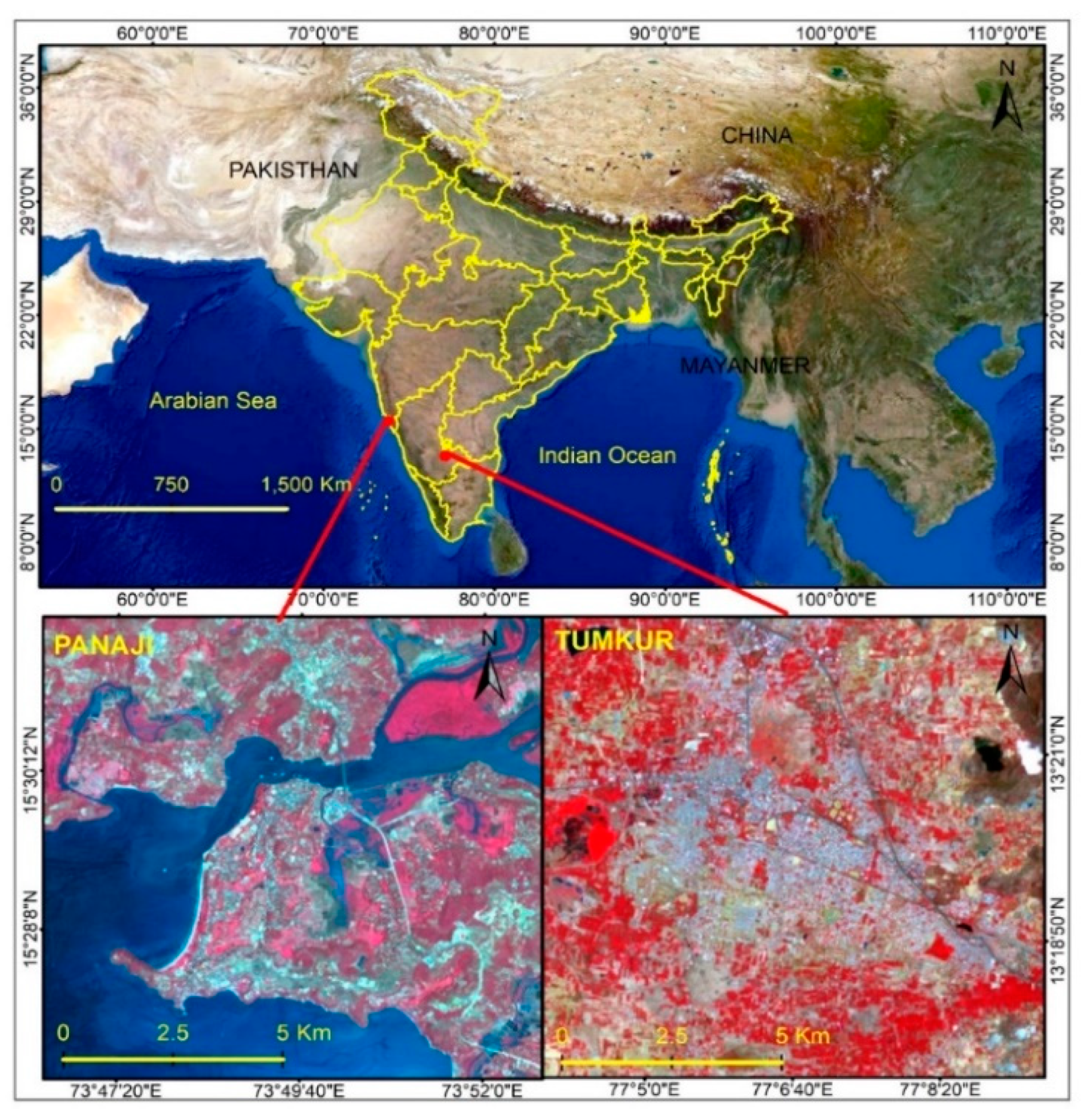
Panaji and Tumkur cities were chosen for this study by considering several factors, such as their geographic location, population, and green space cover. Apart from the disparate geographical locations of Panaji (a coastal city) and Tumkur (an interior city), various other factors such as population size, gross domestic product (GDP), and climatic factors were considered. In 2015, both these cities were designated to be developed as smart cities under the National Smart Cities Mission [50]. Panaji, as a coastal city, is highly vulnerable to sea-level rise issues via climate change impacts. Located in the interior part of India, Tumkur city is rapidly industrializing and recognized as an important National Investment and Manufacturing Zone (NIMZ) by the Government of India. Panaji city is the capital of Goa state and located at a latitude of 15°29′48.3972″ N and a longitude of 73°49′40.1772″ E. Tumkur city is located in the southeastern part of Karnataka state at a latitude of 13°20′17.7468″ N and a longitude of 77°6′5.0760″ E. Figure 1 illustrates the locations of the Panaji and Tumkur cities in India.
In Panaji city [51], despite its strength of compact form and mixed land-use, the most noted weakness listed is a lack of adequate and reliable public transport facilities, both within Panaji and for connecting outgrowth areas to Panaji. The main opportunity is the use of mangroves and a network of creeks as natural resources. These blue-green infrastructures can provide ecosystem services to help mitigate the impacts of threats of urban development and climate change events like sea level rise. Due to rapid urbanization, the city’s environmental resources are noted to get adversely impacted, potentially lowering the city’s resilience to various natural disasters. Notably, there are serious concerns of heavy losses as well as unsustainable and chaotic situations due to many parameters (impending sea level rise, severe traffic congestion, troubled pedestrian mobility, increased population and vehicles, citizens’ health and livability, and resulting air/noise pollution). It is cautioned that the eventual collapse of the existing infrastructure network will occur if appropriate measures are not taken. However, there is no mention in the city development plan on what the LULC changes can bring about or how the new developments would create UHIs or affect the LST.
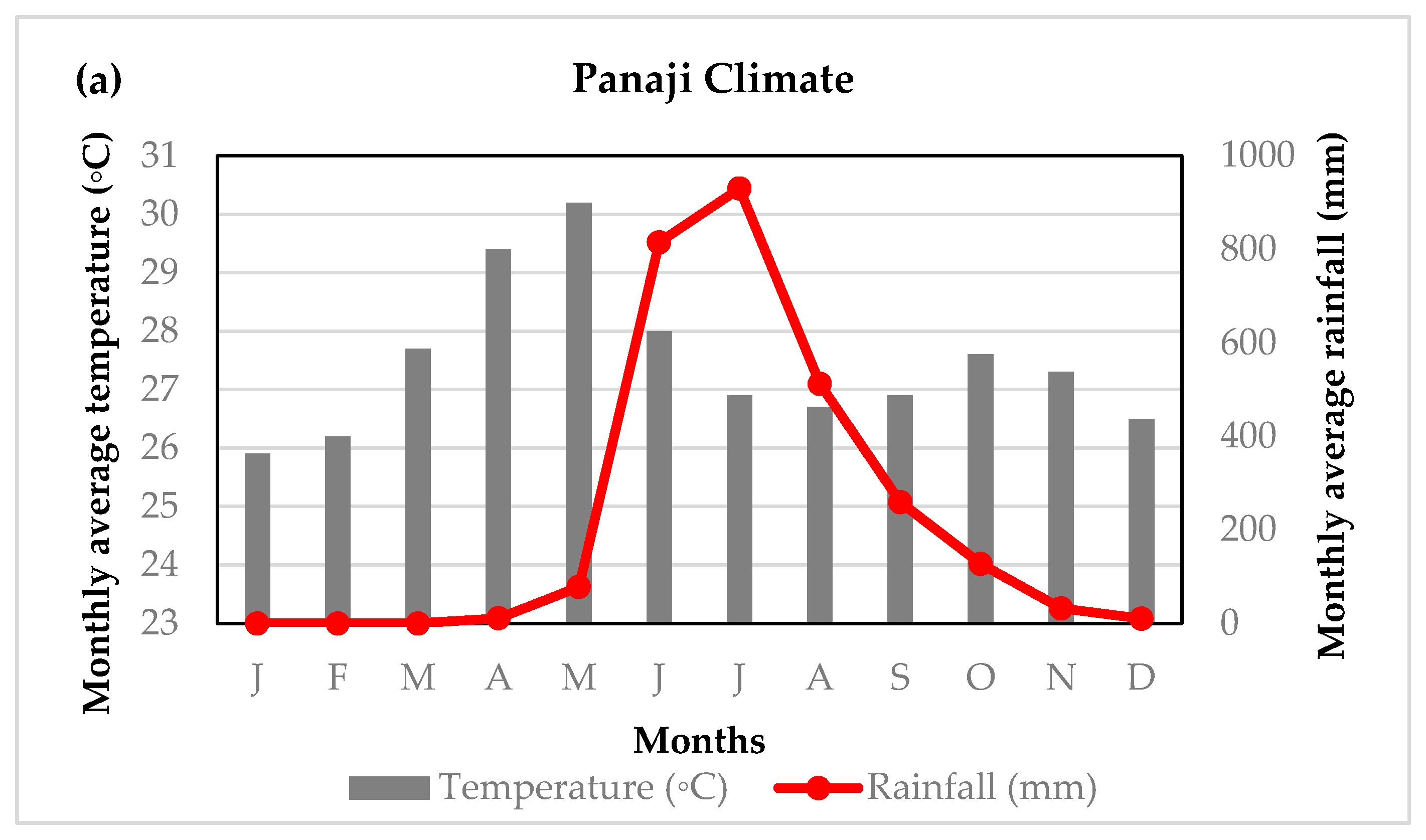
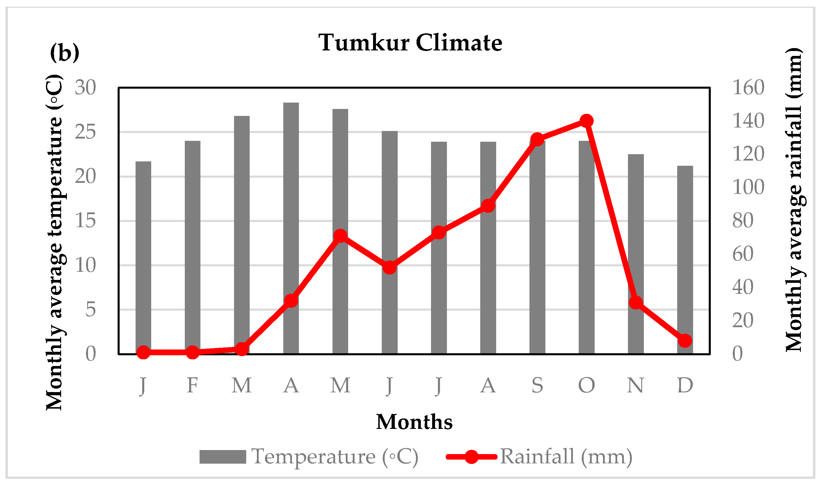
The coastal city of Panaji experiences a tropical climate, with the annual average temperature being 27.4 °C [52]. Temperatures start rising from January to a peak of around 34 °C in April, the hottest month (Figure 2a). Thereafter, it declines during the monsoon months of June–September. The average annual rainfall of Panaji is 2774 mm. The city receives over 85% of the total rainfall during June–September. January is the coldest month with a temperature below 26 °C. The predominant climate in Tumkur is defined as a local steppe climate, with very little rainfall throughout the year [53] and an annual mean temperature of 24.4 °C (Figure 2b). The average annual rainfall is 630 mm in Tumkur and October is the wettest month with 140 mm of precipitation [53]. A comparative account of the major features of these cities is furnished in Table 1.
With 17 parks in the city limits maintained by the Corporation of the City of Panaji (CCP) and the Forest Department, Panaji city (excluding the areas under the CCP) has about 0.80 km2 under green cover [54]. The natural marshy lands and mangroves along the waterfront add to natural, non-curated green areas and act as barriers to prevent monsoonal flooding. The Bhagwan Mahaveer Park maintained by the Forest Department, is the largest green patch in the city. The other 16, mostly small-sized parks plus public gardens, including the forest nursery and roadside plants, add up to about 5% of the green cover.
In Tumkur city, under the Smart City Initiative, there are plans to increase the number (/area) of green spaces. There are four large-sized parks (≥5 ha (≥0.05 km2)) in the city maintained by Tumkur Urban Development Authority (TUDA). A 10 ha (ha) (0.1 km2) newly developed Amanikere Park on the area recovered by landfilling the Amanikere irrigation tank. Further, new roads being laid under the Smart City Development Initiative have walk paths and divider lanes. Suitable plantations on both sides of, and on, the divider in the middle are being made. Unlike the coastal city of Panaji where the monsoonal rains help the green spaces to sustain for quite long periods with once a fortnight watering, Tumkur city in the interior region receives insufficient rainfall. As a result, the existing UGS need watering at least once every week in sufficient quantities to meet up losses, including those occurring through dispersals into the soil.
Panaji and Tumkur are part of the National Smart Cities Mission by the Government of India to make them citizen-friendly and sustainable [50]. The Smart Cities Mission initiated in 2015 has inclusive aims by considering all factors essential for sustainable urban development [55]. Necessary infrastructure elements in a smart city listed by Prakash [55] include adequate water supply, stable assured electricity supply, sanitation (including solid waste and wastewater management), efficient public transport, ease of urban mobility, affordable housing, IT connectivity and digitalization, good governance, sustainable environment, safety and security of citizens, good healthcare, and education/employment opportunities.
3. Data and Methods
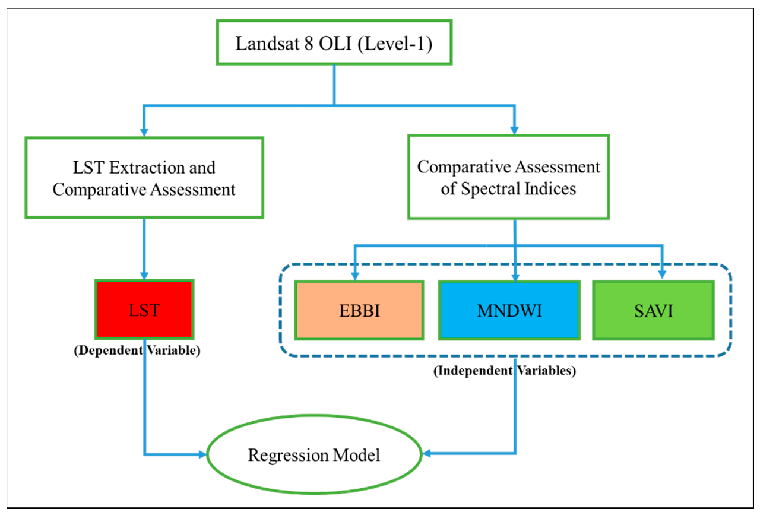
With the introduction of thermal remote sensing, LST information is available from a series of satellite sensors (such as Landsat, MODIS, and ASTER) that cover a wide range of the Earth’s surface. Compared to air temperatures collected from weather stations, thermal imagery provides full spatial coverage at various temporal scales [56]. Figure 3 shows the flowchart of the methodology adopted in this study.
3.1. Satellite Data
Landsat-8 satellite data was used to evaluate the response of different land covers on LST. Landsat 8 satellite has Operational Land Imager (OLI) and Thermal Infrared Sensor (TIR). There are nine spectral bands from bands 1 to 9 and two spectral bands from bands 10 to 11 in OLI and TIRS sensors, respectively. Bands 10 and 11 provide atmospheric rectifications for the thermal inferred data [57]. Two Landsat-8 OLI/TIRS data of the Tumkur and Panaji areas in 2019 were acquired from https://earthexplorer.usgs.gov/ [58]. Table 2 provides details of Landsat-8 data used in this study.
3.2. Field Data
In this study, field surveys were conducted during January–February 2019 to collect ground-truth data for the LULC classification and validation. In the field survey locations of the UGS, built-up areas were marked with the help of a Global Positioning System (GPS) device (Gamin 60x). Various city development offices were also visited to collect secondary information about the landscape, UGS, and city plans. Field surveys were aimed to understand the problems related to LULC patterns in these urban areas and management plans in place to address these problems in both of these upcoming smart cities.
3.3. Methodology
3.3.1. Image Pre-Processing
The analysis in this study only included the ~98 km2 buffer area from both city centers and Landsat data were clipped for further analysis. Atmospheric correction was done prior to image processing. The aim of atmospheric correction was to derive a good estimate of the true at-ground upwelling radiance [59]. The FLAASH (Fast Line-of-sight Atmospheric Analysis of Spectral Hypercubus) model was implemented in the ENVI 5.3 platform provided by Harris Corporation in Melbourne, FL, USA.
3.3.2. Enhanced Built-Up and Bareness Index (EBBI)
Remote sensing techniques provide an efficient and cost-effective approach to monitor the expansion of the built-up area, in comparison to other traditional approaches [13]. Previous studies used different indices for the extraction of desired land features. For example, the Normalized Difference Built-up Index (NDBI) was proposed by Zha [60] for Landsat Thematic Mapper (TM) images, the Built-up Area Extraction Index (BAEI) was proposed by Bouzekri [61] for highlighting built-up areas in Landsat-8 image, improved NDBI was proposed by He [62] as a semi-automatic approach to extract built-up area, and the Enhanced Built-Up and Bareness Index (EBBI) for highlighting built-up land and bare land was proposed by As-syakur et al. [34]. Application of the aforementioned indices depends on the study purpose, surface characteristics, accuracy level, and satellite image physiognomies. In this study, we used the EBBI index for extracting built-up and bare land areas.
A recent study by Li et al., [63] revealed that EBBI is an effective method for extracting built-up area and bare land cover. In view of this, to distinguish the effect of LST on vegetation cover from the land cover altered due to human-induced activities (built-up) and bare land together, we used the EBBI index for extracting built-up and bare land. Hence, both bare land and built-up area were found to be resulting from urban activities. EBBI is derived using the following equation:
where SWIR1, NIR, and TIR represent the band-6, band-5, and band-10 of Landsat-8 data, respectively.
3.3.3. Modified Normalized Difference Water Index (MNDWI)
Waterbodies can be extracted by using the spectral information of satellite images. Compared to other surface objects, water bodies show a weak spectral reflectance in most of the wavelengths. In this research, we used the band threshold method using band-3 (Green) and band-6 (Mid–Infrared/SWIR1) of Landsat-8 images proposed by Xu (2006) which is the modified index of NDWI proposed by McFeeters (1996) for highlighting water bodies [33], who suggested that water information using the NDWI is often mixed with built-up land noise, resulting in an overestimation of extracted water bodies’ areas. MNDWI can provide better results as compared to NDWI. Therefore, MNDWI was used in this study. MNDWI is derived from the following equation:
3.3.4. Soil Adjusted Vegetation Index (SAVI)
The Soil Adjusted Vegetation Index (SAVI) is a useful index for extracting urban area vegetation information. It was proposed by Huete [64], takes into account the optical soil properties on the plant canopy reflectance, and gathers information for a small amount of vegetation. The use of SAVI is an approach by which spectral indices are calibrated, so that soil substrate variations are effectively normalized without influencing vegetation measures [64]. An understanding of soft surface spectral properties, as well as their behavior and interactions with plant life and water, is crucial to development [65]. Therefore an ‘adjustment factor’ is used for measuring SAVI with varying vegetation density. A single adjustment factor (L = 0.5) was adopted in this analysis to shrink soft (moisture, organic inputs, erosion, and cultivation) noise considerably throughout the range in vegetation densities. SAVI, involving a constant L to the NDVI equation with a range of −1 to +1, is expressed as follows:
Two or three optimal adjustments for L constant (L = 1 for low vegetation densities; L = 0.5 for intermediate vegetation densities; L = 0.35 for higher densities) were suggested by Huete [64] wherein NIR and Red represent the band-5 and band-4 of Landsat-8 data, respectively.
3.3.5. Land Surface Temperature (LST)
The land surface temperature was calculated using the standard methodology. Based on Weng et al., [12], a two-step process was followed to derive the brightness temperature of the land. The DN values of each Landsat image band were scaled from the total radiance calculated to byte values before media output using the gain and bias (offset) values given for each group. The DN values can be transformed back to the radiance units using the following formula:
where ML represents the band-specific multiplicative rescaling factor and AL represents the band-specific additive rescaling factor. ML and AL can be obtained from the header file of the satellite data.
Radiance (Lγ) = ML ∗ Band 10 + AL
Once the DN was converted to radiance values, we calculated the brightness temperature (Bt) using the following equation:
where k1 = Band-specific thermal conversion constant (K1_CONSTANT_BAND_10) and k2 = Band-specific thermal conversion constant (K2_CONSTANT_BAND_10), we can find the constant from the image header file.
Thereafter, the Surface emissivity (ε) was calculated using the proportion of vegetation coverage (PV). The following two equations were used:
Surface emissivity , where 0.004 and 0.986 are the correlation values of surface emissivity.
After calculating the brightness temperature and surface emissivity, the LST was calculated by using the following equation:
where 0.00115 and 1.4388 are the correlation values of LST.
3.4. Statistical Analysis
To find out the significance of changing urban green cover and the impact on urban microclimate, we developed a regression model. Regression analysis is a type of predictive modeling technique that investigates the relationship between a dependent (target) and independent variable (s) (predictor) [66]. It expresses the strength of the impact of multiple independent variables on a dependent variable [67]. In this study, “Stepwise Regression” model was used. The selection of multiple independent variables was done with the help of an automatic process without human intervention. This technique basically fits the regression model by adding/dropping co-variates, one at a time, based on a specified criterion. In this study, LST was the dependent variable; while EBBI, MNDWI, and SAVI were the independent variables. The aim of this modeling was to investigate the significance of the presence of built-up area, water bodies, and vegetation on LST in the urban area. Equation (8) illustrates the regression model.
where αo, β, x, and e represent the constant, coefficient, variables, and significant error, respectively.
4. Results
The widely employed Spectral Indices is a reliable indicator for closely observing Earth surfaces using remote sensing technology. The EBBI is the built-up and bare land index that applies near-infrared (NIR), short wave infrared (SWIR), and thermal infrared (TIR) channels simultaneously [34]. Vegetation has a high reflectance in NIR, but the reflectance of built-up or bare land is low. In contrast, TIR has high reflectance to detect built-up areas as compared to vegetated areas, thus making it effective for built-up areas mapping [68].
4.1. Comparative Analyses of Various Indices
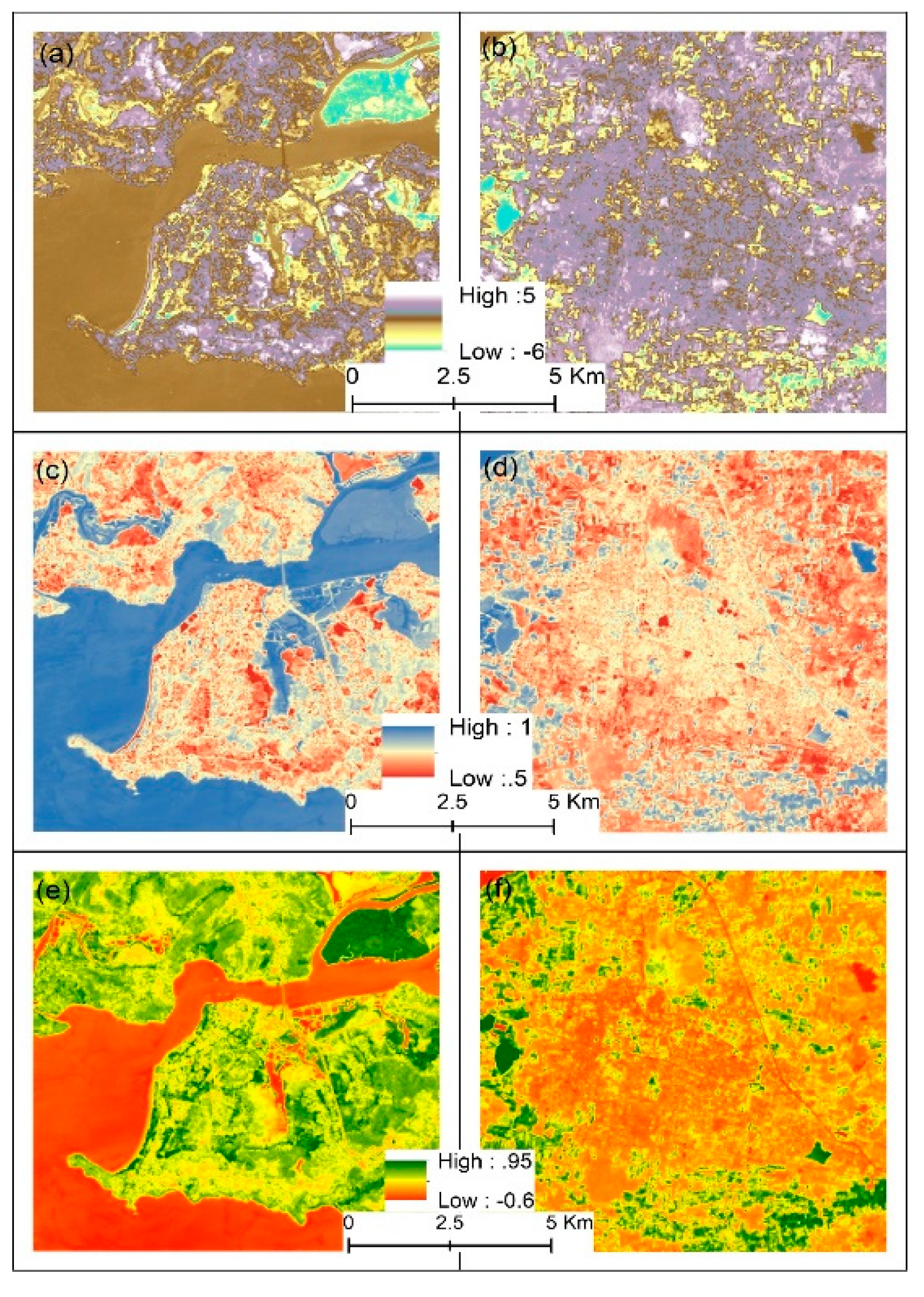
Spectral Indices utilize spectral reflectance properties to distinguish different LULC classes present in the study area. EBBI, MNDWI, and SAVI indices as discussed in Section 3.3 were calculated using Landsat-8 data. Later, a non-parametric support vector machine (SVM) classifier was used to extract LULC to validate the findings of indices. Figure 4 shows the EBBI, MNDWI, and SAVI indices for both Panaji and Tumkur cities.
Visual interpretation of extracted spectral indices for EBBI is useful to recognise lower reflectance in Panaji (Figure 4a) than Tumkur (Figure 4b). It can, therefore, be inferred from the images that EBBI is high for the Tumkur area, indicating that the percentage of the built-up and bare land area is more than twice that of Panaji. The MNDWI also depicts a much higher waterbody coverage area in Panaji (Figure 4c) than in Tumkur (Figure 4d). Most of the area in Panaji is surrounded by water bodies compared to that of Tumkur (Figure 4c). Similarly, the SAVI is quite high for Panaji (Figure 4e) compared to Tumkur (Figure 4f). In Panaji, the vegetation is distributed evenly within the city area. Besides, a higher reflectance value of SAVI is witnessed in the Panaji area than in Tumkur. Panaji city has much more evenly spread green areas than can be visualized for Tumkur city, where green areas are distributed rather sparsely, unevenly, and mostly in the peripheral parts of the city. A clear gradient from the city core to the peripheral area is discernible (Figure 4f). There is a tradeoff between urban ecological features (green spaces and water bodies) and built-up areas. Therefore, Tumkur city needs a better urban green space management plan for smart city development to improve its ecosystem services.
4.2. Land Use Land Cover (LULC)
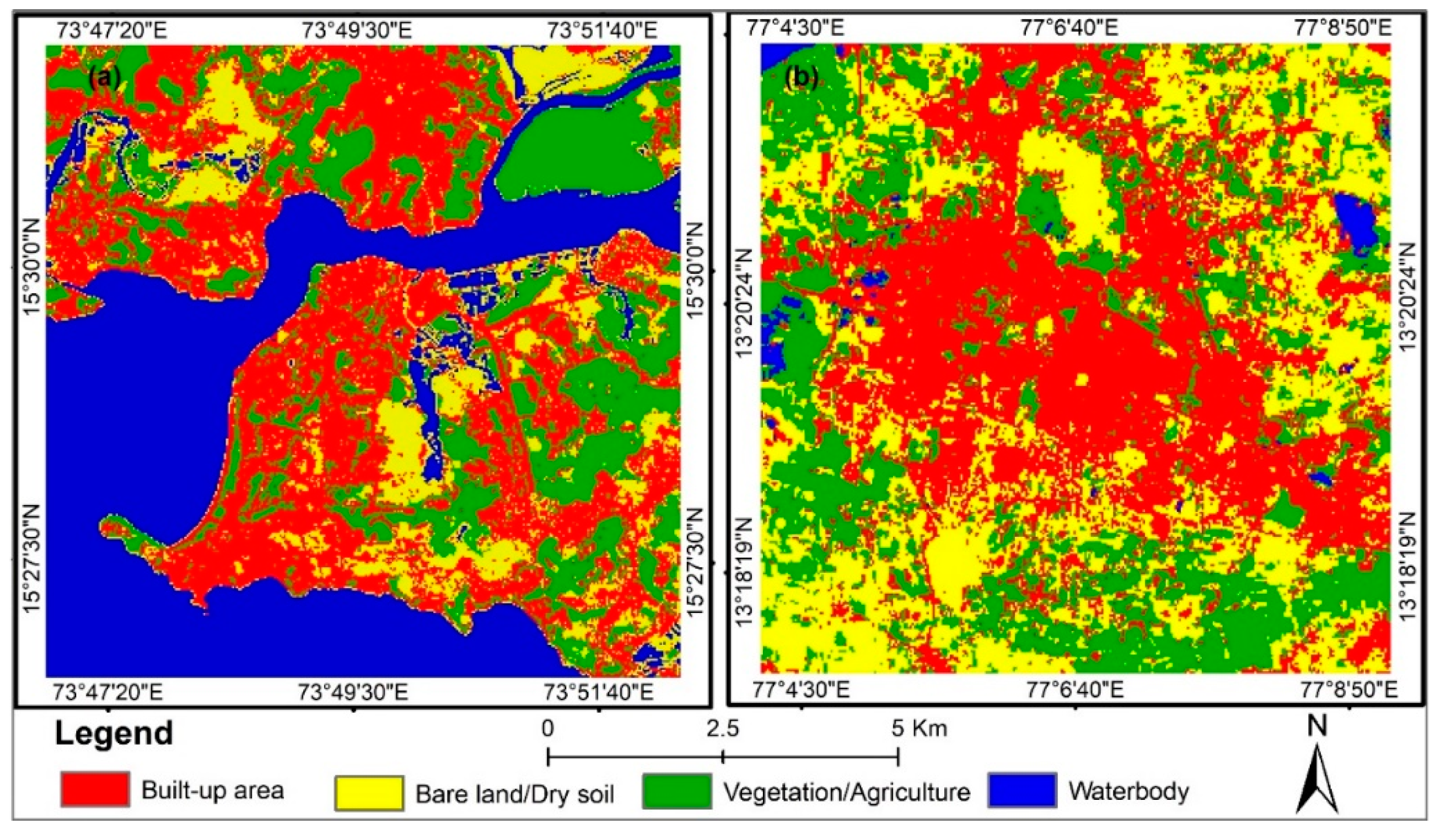
To examine the spatial pattern of LULC in Panaji and Tumkur, SVM classification was performed in ENVI for 2019. The LULC map was cross-checked with recent Google images. A total of 179and 251 training samples were taken for Panaji and Tumkur, respectively. For the validation of LULC map, 120 and 95 samples were used to validate the results in Panaji and Tumkur, respectively. The classified images showed an overall accuracy of 90.31% and a Kappa coefficient of 0.83 for Panaji and overall accuracy of 89.78% with Kappa coefficient of 0.79 for Tumkur city. Figure 5 illustrates the LULC pattern of the Panaji and Tumkur cities. An accuracy assessment of classified maps was done using a confusion matrix. Appendix A illustrate the overall accuracy of LULC maps and Kappa coefficient based on the confusion matrix. In Tumkur, the built-up class was the most dominant land cover type in 2019, representing 41% of the total area; followed by bare land (33%), vegetation (30%), and water bodies (1%). In Panaji, 32% of the land area is covered with water bodies class; followed by built-up (32%), vegetation (24%), and bare land (12.49%). Table 3 shows the area of various LULC classes in the study area. Most of the area of Panaji is covered by water bodies and vegetation, whereas Tumkur is covered by built-up and bare land. Therefore, the functional characteristic of LULC is completely opposite for the two cities. Tumkur is dominated by the LULC of urban activities, while Panaji is dominated by urban ecological features.
4.3. Land Surface Temperature (LST)
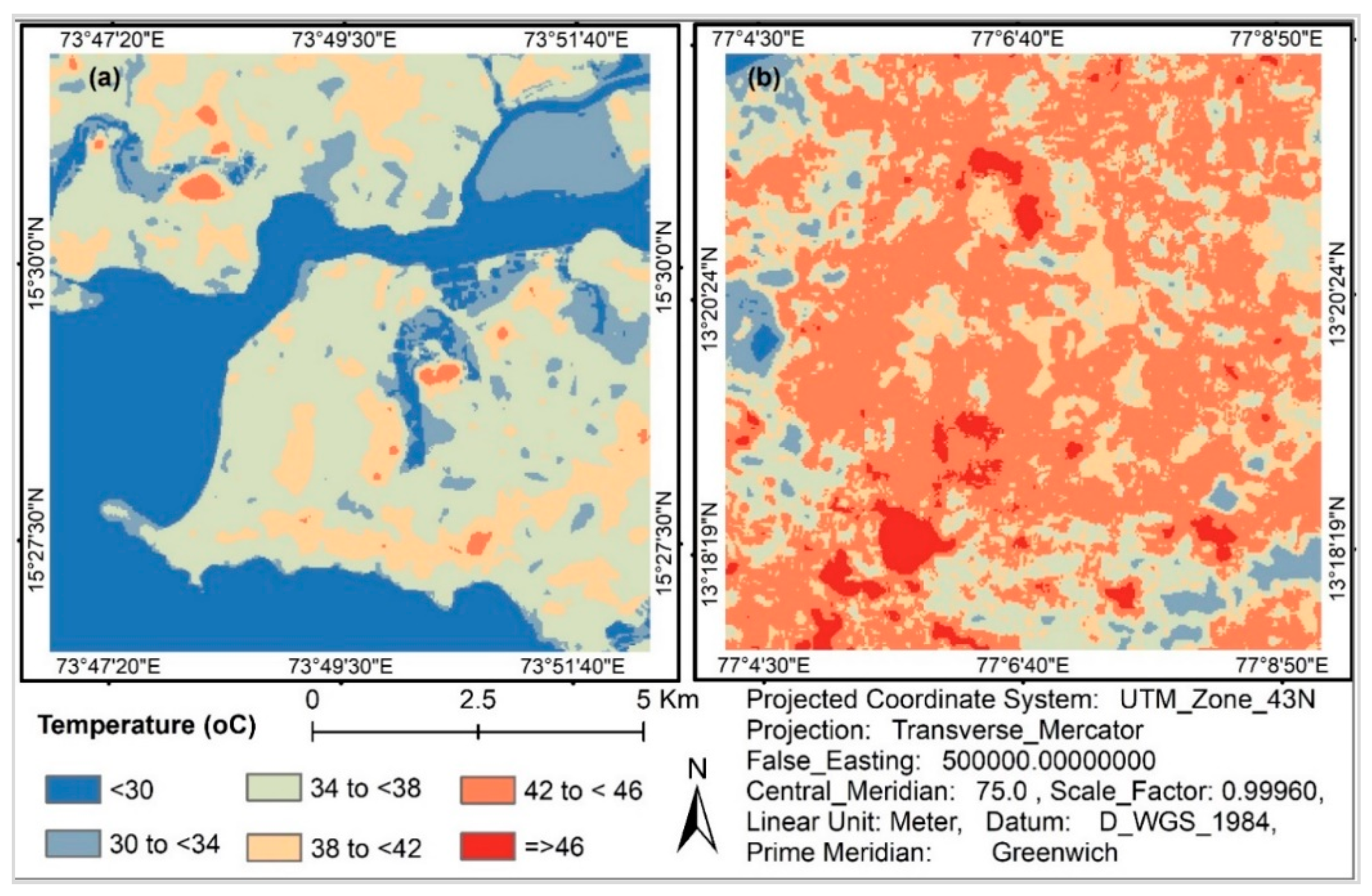
The LST estimated by using the radiative transfer equation algorithm using TIR-band is effective for deducing surface emissivity in the urban landscape [6]. This technique is used to recognize the response of different thermal properties on the Earth’s surface. The response of such thermal properties varies with different landscape patterns, different geographical locations, and climatic conditions such as rainfall, wind speed, etc. Also, the land cover dynamics viz, agriculture/vegetation, waterbody, built-up area, bare land, etc. seriously affect the LST variations [6]. The LST images for Panaji and Tumkur (Figure 6a,b) indicate a temperature range of 34–38 °C in most area of Panaji and 42–46 °C for the most area of Tumkur city The LST pattern in Panaji is largely homogeneous, unlike the quite heterogeneous one of Tumkur. In Panaji, about 35% of the area is covered by water bodies and experiences temperatures < 30 °C. In Tumkur, only a few places close to water bodies and vegetation experience < 30 °C. The maximum LST of (≥) 46 °C is observed in approximately 4% of the land area of Tumkur city. On the other hand, in Panaji, the LST maximum of 42 °C to 46 °C is in < 1% of the land area. The maximum and minimum LST differences are lower in Panaji (12 °C) and higher in Tumkur (16 °C).
4.4. Relationship of LST and EBBI, MNDWI, and SAVI
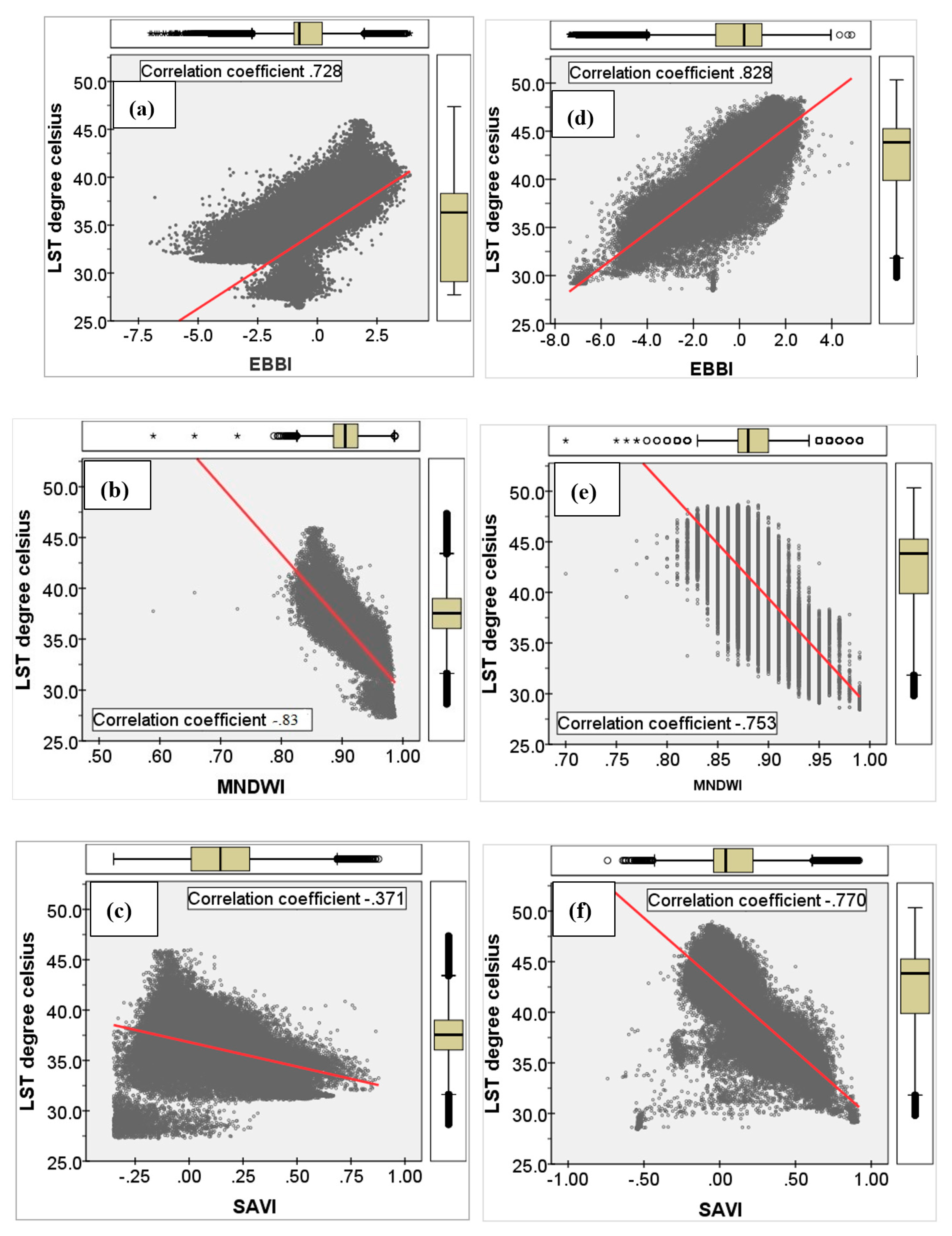
Figure 7 illustrates the non-parametric test with indices of urban features and LST. Generally, LST bears a negative relationship with SAVI and MNDWI, and a positive relationship with EBBI. The 30 m × 30 m pixel-based correlation coefficient values between LST and SAVI, MNDWI and EBBI were significant (P < 0.01). The EBBI had a strong positive correlation with LST among these three indices for both cities (Figure 7a,d). This implies that both bare land and built-up are causes of high LST in both cities. The SAVI and MNDWI indicate a strong negative correlation with LST for both cities (Figure 7b,c,e,f). A weak correlation of −0.37 between LST and SAVI is seen for Panaji compared to Tumkur with a strong correlation of −0.75. This may be due to a low UHI effect in Panaji compared to Tumkur. Besides, Panaji city being located near the seashore and also interspersed by water channels, experiences minimal LST differences.
4.5. Regression Model
The multivariate regression model derived in this analysis is useful to denote the relationship between LST and EBBI, MNDWI, and SAVI. LST being the dependent variable, is affected by EBBI, MNDWI, and SAVI (the independent variables). The adjusted R2 in the linear regression model is 0.698 (with standard error 1.407) for Panaji city. A high 0.582 Durbin-Watson d (within the two critical values of 0 < d < 2) signifies a strong linear auto-correlation. Similar to Tumkur, the highly significant F-test (P < 0.0001) ascertains that the model explains a significant amount of the variance in LST. By subjecting all variables to multiple linear regression, it is inferred that SAVI, MNDWI, and even EBBI serve as significant predictors as there was a high level of significance (P < 0.0001) between LST and all three independent variables. The significance level for SAVI, MNDWI, and EBBI is less than 0.0001. We also observe that the impact of EBBI and MNDWI is higher than SAVI by comparing the standardized coefficients (beta coefficient for SAVI = −0.168, MNDWI = −1.06 and EBBI = 0.00338). From the multiple linear regression model, the following relationship is predicted among LST and EBBI, MNDWI, and SAVI for Panaji city with unstandardized coefficient of the variables:
LST (Panaji) = 114.531 + 0.563 EBBI − 86.349 MNDWI − 2.206 SAVI.
For Tumkur city, the adjusted R2 value is 0.716 (with a standard error of 1.97). The Durbin-Watson d being 0.578 brings forth a strong linear auto-correlation between different variables used for multiple linear regression analyses. With the F-test revealing a highly significant (P < 0.0001) relationship, it is confirmatory that this model explains a significant amount of the variance in LST for Tumkur city. By forcing all variables into the multiple linear regression, it can be discerned that both SAVI and MNDWI are significant predictors. The level of significance for SAVI and MNDWI is a high of <0.001, while for EBBI, it is a low of 0.058. We also observe that the impact of SAVI and MNDWI is higher than EBBI by comparing the standardized coefficients (beta coefficient for SAVI = −0.483, MNDWI = −0.439 and EBBI = 0.016). From this multiple linear regression model, the following relationship among LST and EBBI, MNDWI, and SAVI is predicted for Tumkur city with an unstandardized coefficient of variables.
LST (Tumkur) = 97.80 + 0.036 EBBI − 62.987 MNDWI − 8.272 SAVI
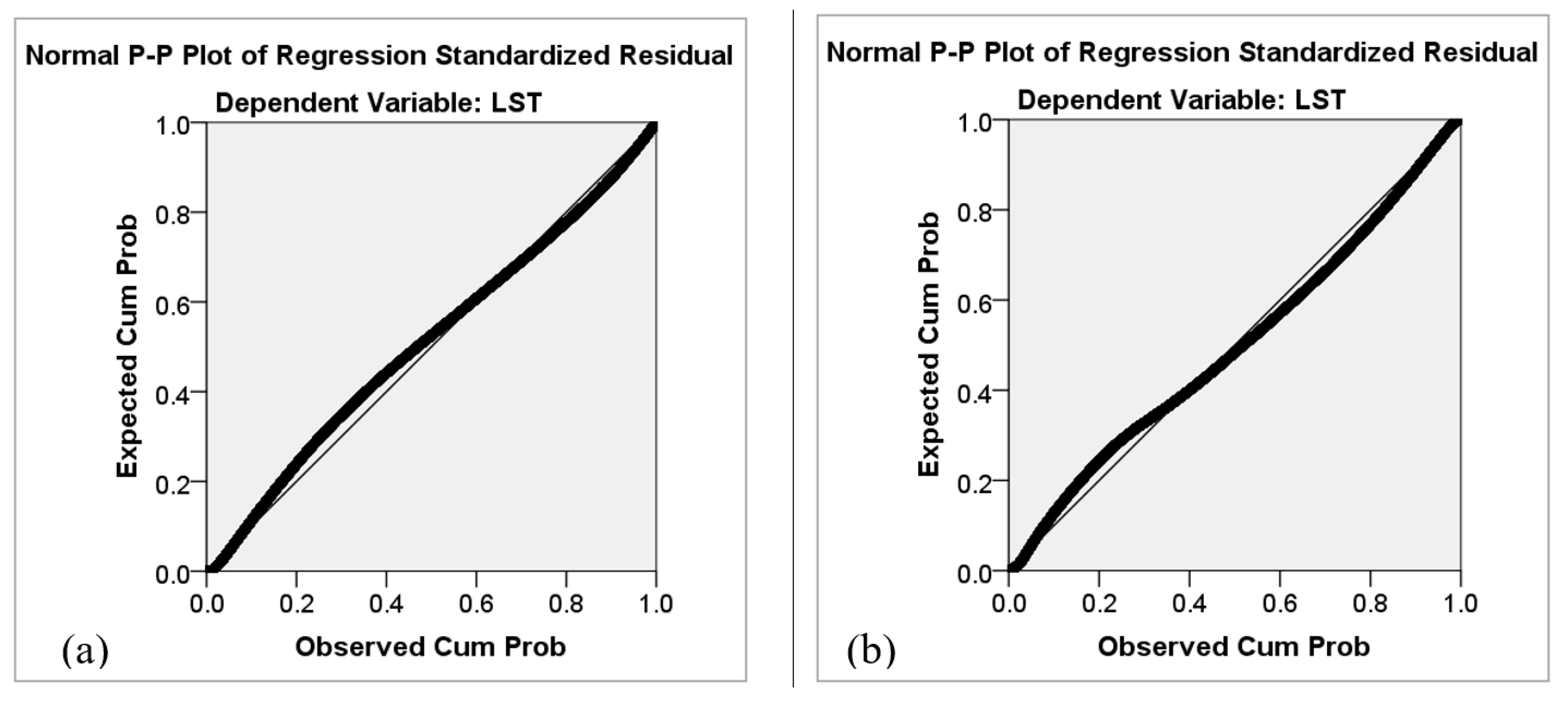
From checking for normality of residuals with a normal P-P plot (Figure 8), it can be inferred that the points generally follow the normal diagonal line with no strong deviations, indicating a normal distribution of residuals for both cities. Apparently, the regression model developed in this analysis is applicable only for these cities. Owing to geomorphological heterogeneity of different cities, future studies can consider inputs of land cover variations using this strategy.
5. Discussion
This comparative study focused on spectral indices and their influence on LST in the coastal city of Panaji and the interior city of Tumkur slated for development as smart cities. Low urban landscape patterns in Panaji are mixed with built-up areas and vegetation. There is a possibility of confusion towards extracting built-up areas using EBBI approach. Ahmed et al., [69] reported that the tremendous pressure of urbanization on the peripheral area of a city leads to the conversion of non-built-up areas (green area, agriculture land, waterbody) into built-up areas. The first step of such a conversion process is ecosystem sensitive land cover to bare land and finally, it is replaced by built-up area [70]. In this context, Tumkur is environmentally more vulnerable than Panaji due to the presence of more bare land.
MNDWI can extract the water information efficiently from both built-up and non-built-up areas. It can dampen the built-up land information effectively while highlighting water information and can accurately extract the water bodies information [33]. However, from a statistical perspective, when most land cover types differ from each other, the MNDWI’s efficiency in identifying water, saturated soil, or different water content of the vegetation can lead to misclassification. Biggs et al., [71] emphasized that the presence of water bodies (ponds, small lakes, low-order streams, ditches, or springs) are critical for freshwater biodiversity and are increasingly recognised for their role in a variety of ecosystem services as well as the aquatic ecosystem. Jackson et al., [72] reported that MNDWI is positively correlated with vegetation water content and useful for assessing the extent of strains of drought in any area. In Tumkur, where the availability of water bodies is minimal, it can be suggested that the functioning of urban ecosystem services is negatively affected, and vegetative areas might experience water stress during summer. The high value of MNDWI in Panaji is related to high vegetation water content and it might help vegetation to have less water stress during summer.
SAVI is the measuring index for vegetation or green spaces which has more functional value for the urban ecosystem. The significant coefficient of the regression model illustrates that MNDWI and SAVI are accountable for combatting LST. Although the percent share of SAVI and MNDWI is higher than that of built-up and bare land, MNDWI was the most significant predictor for controlling LST in Panaji, while SAVI was the important predictor for Tumkur.
Surface temperature also has a direct interaction with LULC characteristics [73]. Therefore, the analysis of the relationship between LULC and LST is crucial in order to understand the effects of LULC on UHI. The land cover dynamics are accountable for elevated or decreased LST. Higher/significant correlation coefficient values between LST and EBBI, MNDWI, and SAVI for Panaji and Tumkur cities clearly reflect that both bare land and built-up area cause, accelerate, and sustain higher LSTs. It can be inferred that the existing coverage of water bodies in Panaji seems to dampen the LST to a greater extent when compared to Tumkur. Both LULC and spectral indices, as well as the observed higher LST in Tumkur, signify inefficient ecosystem services more than a better service could in Panaji city. With much lower vegetation cover in Tumkur, the degree of absorption of solar radiation by built-up and dry soil drastically elevates the LST and alters the conditions of the near-surface atmosphere [74] over Tumkur city.
Tran et al., (2017) [8] inferred that absolute LST is useful in characterizing UHIs on a short-term basis (particular date) but is not effective in comparing spatial patterns of UHI through time. To ensure that LST values retrieved from different images are comparable, Walawender et al., (2014) [75] had proposed the use of normalized LST to investigate the LST spatial distribution in relation to LULC. Many earlier studies [76,77,78] had emphasized that the simulation of future LST, based on LULC, helps in mitigating UHIs effects and in adopting new strategies and policies in land use planning and urban design to reduce/control the UHIs effect. In view of such possibilities, it can be inferred from our analyses that both the cities are prone to increased LST for reasons mentioned earlier. Further, as Guo et al., (2015 [79] and 2016 [80]) recommend, these cities would be better placed for LST prediction by taking into account the complex landscape structure and urban morphology heterogeneity. Results of this study showcase the effectiveness of the spectral indices derived in identifying the LST differences within the study area and in marking UHIs. These could provide crucial feedback to planners and policy-makers for the inclusion of UHIs mitigation measures.
In general, LST is negatively correlated with SAVI and MNDWI and positively correlated with EBBI. But, these relationships tend to change with UHI [70]. With both SAVI and MNDWI bearing a stronger correlation with LST in both the cities, it can be suggested that the impact of UHI is strong in at least over 50% of the areas. Guha et al. [81] reported that vegetation areas have a much better negative correlation with LST, but these relationships gradually weaken with the increase of the heterogeneous surface features. Although Panaji has a smaller urban area compared to Tumkur, the large water body, forest cover, and hilly features render Panaji city as a more heterogeneous surface than Tumkur city, which is located in the plains of India’s interior. A weak correlation (R2 = −0.37) in Panaji city and a significant correlation (R2 = −0.75) between LST and SAVI in Tumkur city can be taken to suggest that there is a lower UHI effect in Panaji city than in Tumkur city, a fact that can be confirmed through visual analyses of the images (Figure 5). In Panaji city located near the sea, the water channels surrounding the city area are minimizing the LST differences.
Though there is more green cover in Panaji, it is inadequate according to the Urban and Regional Development Plans Formulation & Implementation (URDPFI) guidelines [54]. Currently, existing roadside plants and 17 parks are irrigated by the Public Works Department (PWD) by diverting an unspecified volume of urban drinking water supplies. While over 70% of domestic sewage is claimed to be treated, all the treated water from Tonca sewage treatment plant (STP) is drained into an adjacent polluted creek ‘to improve its water quality’.
In Tumkur, under the Smart City Initiative [82], there are plans to increase the number(/area) of green spaces. Unlike in Panaji where the monsoonal rains help sustain green spaces for quite long periods (with once a fortnight watering), Tumkur, located in the interior region, receives less rainfall. Thus, a 150 km-long canal is planned for potable water supply from River Hemavathi to this rapidly urbanizing, water-scarce city. Besides meeting drinking water demand, the canal is expected to help meet water requirements for existing and planned parks and roadside vegetation. To provide respite from unhealthy LST and UHI impacts, maintenance of existing parks, adding many more new ones, and roadside trees to increase the green cover are vital steps. The fact that urban greening would help overcome the adverse effects of elevated LST [83,84,85] ought to sensitize the development of both Panaji and Tumkur as smart cities. Further, as Thapa and Murayama [86], and Ramaiah and Avtar [87] suggest, green areas must be considered. As reported from Dhaka [88], with the percent share of urban green areas getting reduced due to unplanned urban activities and weak land-use zoning regulations, Tumkur city needs a sound urban green space management strategy.
While some alternative options exist for surface water (such as groundwater, water supply from outside the urban areas, treated urban wastewater), there are no alternatives for green spaces and their services. Green spaces not only control LST, they also provide recreational facilities, beautify the city, contribute to atmospheric oxygen, and purify the air for maintaining ecological balance and for the upkeep of biodiversity [89]. From a significant positive spatial autocorrelation observed between LST and greenspace area within the chosen section/s of expansive Beijing, Li et al., (2012) [90] suggested that green spaces bring down summertime LST by 5 °C.
In Tumkur city in particular, UGS can reduce temperatures through direct shading and evapotranspiration, and as Tyrväinen et al., (2005) [91] recommended, they can create a local cool island within this sprawling urban area. With proper maintenance practices, including the use of treated wastewater, the existing vegetation in its 400 plus listed parks in addition to new ones (including roadside plantation) can also achieve many other environmental benefits such as reduced rainwater runoff, greater urban biodiversity, and improved aesthetics [92,93]. Although there may not be a linear relationship between the cooling effect and the size of greenspace [94], there would be discernible cooling effects in specific locations with denser vegetation. These desirable services are necessary for a high-quality living environment. The use of advanced remote sensing techniques can help in the development and maintenance of UGS as part of the smart city programs and implementation of SDGs 11.
6. Conclusions
Any existing urban fabric would lead to rapid changes in the urban environment whenever altered. This, in turn leads to deviations in urban settings in a variety of ways. Thus, urban settlements ought to plan and create facilities/amenities that are ergonomic, long-lasting, and encompassing. This study compares two upcoming smart cities (Panaji and Tumkur) in India using landscape sensitivity analysis and its influence on LST. The urban factors such as EBBI, SAVI, and MNDWI influence the LST in both cities. The study reveals that water bodies and green spaces are actively responsible for dampening LST. The performances of LST dampening depends on the maximum share of cooling surfaces (water bodies and green spaces) in the study area. In the Panaji, the correlation coefficient between EBBI, SAVI, and MNDWI with LST is about 0.72, −0.37, and −0.83, respectively. On the other hand, in the Tumkur, the correlation coefficient between EBBI, SAVI, and MNDWI with LST is about 0.829, −0.77, and −0.753, respectively. The multivariate regression model reveals that in the Tumkur, the adjusted R2 of the developed model is 0.716 with the standard error 1.97 and in the Panaji, the adjusted R2 of the developed model is 0.698 with the standard error being 1.407. This study did not consider the local climate issues such as wind speed, rainfall, topography, and functional activities of the urban area (e.g., industrial and economic activities, building densities, transportation) may reinforce the findings. Therefore, there is a need to consider these limitations open for further investigations. The use of advanced remote sensing techniques can help to maintain urban green spaces for healthy and livable city development. The analyses of this study would serve as guidelines for an in-depth investigation of the significance of urban green spaces in controlling/reducing urban heat island effects.
Author Contributions
Conceptualization, M.R., R.A., M.M.R.; methodology, M.R., M.M.R.; formal analysis, M.R., M.M.R., R.A.; investigation, M.R.; writing M.R., M.M.R., R.A.; writing—review and editing, M.R., R.A. All authors have read and agreed to the published version of the manuscript.
Funding
No external funding was obtained beyond that discussed below.
Acknowledgments
The first author is grateful to the Faculty of Environmental Earth Science, Hokkaido University for facilities and JASSO for the scholarship support. We are thankful to the United States Geological Survey (USGS) for providing Landsat satellite data and the Global Challenge Research Funds (GCRF) of the University of Glasgow. The authors acknowledge the support of the urban development departments of Panaji and Tumkur cities for providing necessary data and information. Constructive suggestions offered by anonymous reviewers helped improve and revise the manuscript.
Conflicts of Interest
The authors declare no conflict of interest.
Appendix A
Table A1 and Table A2 show the results of the accuracy assessment of LULC classification based on Landsat-8 data acquired in 2019 for Panaji and Tumkur.

Table A1.
Confusion matrix of the 2019 LULC map of Panaji.
| Built-Up Area | Bare Land | Water Body | Vegetation/Agriculture | Classification Overall | Producer’s Accuracy | |
|---|---|---|---|---|---|---|
| Built-up area | 20 | 3 | 0 | 0 | 23 | 86.95% |
| Bare land | 2 | 18 | 0 | 0 | 20 | 90.00% |
| Water body | 0 | 0 | 24 | 3 | 27 | 88.89% |
| Vegetation/agriculture | 0 | 0 | 2 | 23 | 25 | 92.00% |
| Overall Truth | 22 | 21 | 26 | 26 | 95 | |
| User’s accuracy | 90.90% | 86.72% | 90.30% | 88.46% | ||
| Overall Accuracy | 90.32% | |||||
| Kappa coefficient | 0.83 |
Table A2.
Confusion matrix of the 2019 LULC map of Tumkur.
| Built-Up Area | Bare Land | Water Body | Vegetation/Agriculture | Classification Overall | Producer’s Accuracy | |
|---|---|---|---|---|---|---|
| Built-up area | 25 | 5 | 0 | 0 | 30 | 83.33% |
| Bare land | 4 | 23 | 0 | 0 | 27 | 85.18% |
| Water body | 0 | 0 | 27 | 5 | 32 | 84.37% |
| Vegetation/agriculture | 0 | 0 | 6 | 25 | 31 | 80.64% |
| Overall Truth | 29 | 28 | 33 | 30 | 120 | |
| User’s accuracy | 86.21% | 82.14% | 81.81% | 83.33% | ||
| Overall Accuracy | 83.33% | |||||
| Kappa coefficient | 0.778 |
References
- Koomen, E.; Rietveld, P.; Bação, F. The third dimension in urban geography: The urban-volume approach. Environ. Plan. B Plan. Des. 2009, 36, 1008–1025. [Google Scholar] [CrossRef] [Green Version]
- Estoque, R.; Murayama, Y.; Tadono, T.; Thapa, R. Measuring urban volume: Geospatial technique and application. Tsukuba Geoenviron. Sci. 2015, 11, 13–20. [Google Scholar]
- Wheeler, S. Planning for Sustainability; Routledge: Abington, UK, 2004; ISBN 0203300564. [Google Scholar]
- Hua, A.K.; Ping, O.W. The influence of land-use/land-cover changes on land surface temperature: A case study of Kuala Lumpur metropolitan city. Eur. J. Remote Sens. 2018, 51, 1049–1069. [Google Scholar] [CrossRef] [Green Version]
- Amiri, R.; Weng, Q.; Alimohammadi, A.; Alavipanah, S.K. Spatial–temporal dynamics of land surface temperature in relation to fractional vegetation cover and land use/cover in the Tabriz urban area, Iran. Remote Sens. Environ. 2009, 113, 2606–2617. [Google Scholar] [CrossRef]
- Rahman, M.; Avtar, R.; Yunus, A.P.; Dou, J.; Misra, P.; Takeuchi, W.; Sahu, N.; Kumar, P.; Johnson, B.; Dasgupta, R.; et al. Monitoring Effect of Spatial Growth on Land Surface Temperature in Dhaka. Remote Sens. 2020, 12, 1191. [Google Scholar] [CrossRef] [Green Version]
- Naserikia, M.; Asadi Shamsabadi, E.; Rafieian, M.; Filho, W. The Urban Heat Island in an Urban Context: A Case Study of Mashhad, Iran. Int. J. Environ. Res. Public Health 2019, 16, 313. [Google Scholar] [CrossRef] [PubMed] [Green Version]
- Tran, D.X.; Pla, F.; Latorre-Carmona, P.; Myint, S.W.; Caetano, M.; Kieu, H.V. Characterizing the relationship between land use land cover change and land surface temperature. ISPRS J. Photogramm. Remote Sens. 2017, 124, 119–132. [Google Scholar] [CrossRef] [Green Version]
- Liu, W.; Ji, C.; Zhong, J.; Jiang, X.; Zheng, Z. Temporal characteristics of the Beijing urban heat island. Theor. Appl. Climatol. 2007, 87, 213–221. [Google Scholar] [CrossRef]
- Xiao, R.; Ouyang, Z.-Y.; Zheng, H.; Li, W.-F.; Schienke, E.W.; Wang, X.-K. Spatial pattern of impervious surfaces and their impacts on land surface temperature in Beijing, China. J. Environ. Sci. 2007, 19, 250–256. [Google Scholar] [CrossRef]
- Xiao, R.; Weng, Q.; Ouyang, Z.; Li, W.; Schienke, E.W.; Zhang, Z. Land surface temperature variation and major factors in Beijing, China. Photogramm. Eng. Remote Sens. 2008, 74, 451–461. [Google Scholar] [CrossRef] [Green Version]
- Weng, Q.; Lu, D.; Schubring, J. Estimation of land surface temperature–vegetation abundance relationship for urban heat island studies. Remote Sens. Environ. 2004, 89, 467–483. [Google Scholar] [CrossRef]
- Yang, L.; Xian, G.; Klaver, J.; Deal, B. Urban Land-Cover Change Detection through Sub-Pixel Imperviousness Mapping Using Remotely Sensed Data. Photogramm. Eng. Remote Sens. 2003, 69, 1003–1010. [Google Scholar] [CrossRef]
- Rizwan, A.M.; Dennis, L.Y.; Chunho, L. A review on the generation, determination and mitigation of Urban Heat Island. J. Environ. Sci. 2008, 20, 120–128. [Google Scholar] [CrossRef]
- Plocoste, T.; Jacoby-Koaly, S.; Molinié, J.; Petit, R.H. Evidence of the effect of an urban heat island on air quality near a landfill. Urban Clim. 2014, 10, 745–757. [Google Scholar] [CrossRef]
- Alghannam, A.R.O.; Al-Qahtnai, M.R.A. Impact of vegetation cover on urban and rural areas of arid climates. Aust. J. Agric. Eng. 2012, 3, 1. [Google Scholar]
- Ng, E.; Chen, L.; Wang, Y.; Yuan, C. A study on the cooling effects of greening in a high-density city: An experience from Hong Kong. Build. Environ. 2012, 47, 256–271. [Google Scholar] [CrossRef]
- Grover, A.; Babu Singh, R. Analysis of Urban Heat Island (UHI) in Relation to Normalized Difference Vegetation Index (NDVI): A Comparative Study of Delhi and Mumbai. Environments 2015, 2, 125–138. [Google Scholar] [CrossRef] [Green Version]
- Avtar, R.; Tripathi, S.; Aggarwal, A.K. Assessment of Energy–Population–Urbanization Nexus with Changing Energy Industry Scenario in India. Land 2019, 8, 124. [Google Scholar] [CrossRef] [Green Version]
- Lilly Rose, A.; Devadas, M.D. Analysis of Land Surface Temperature and Land Use/Land Cover Types Using Remote Sensing Imagery-A Case in Chennai City, India. In Proceedings of the 7th International Conference on Urban Climate (ICUC-7), Yokohama, Japan, 29 June–3 July 2009; Volume 29. [Google Scholar]
- Weng, Q.; Liu, H.; Lu, D. Assessing the effects of land use and land cover patterns on thermal conditions using landscape metrics in city of Indianapolis, United States. Urban Ecosyst. 2007, 10, 203–219. [Google Scholar] [CrossRef]
- Sannigrahi, S.; Bhatt, S.; Rahmat, S.; Uniyal, B.; Banerjee, S.; Chakraborti, S.; Jha, S.; Lahiri, S.; Santra, K.; Bhatt, A. Analyzing the role of biophysical compositions in minimizing urban land surface temperature and urban heating. Urban Clim. 2018, 24, 803–819. [Google Scholar] [CrossRef]
- Sinha, S.; Pandey, P.C.; Sharma, L.K.; Nathawat, M.S.; Kumar, P.; Kanga, S. Remote estimation of land surface temperature for different LULC features of a moist deciduous tropical forest region. In Remote Sensing Applications in Environmental Research; Springer: Basel, Switzerland, 2014; pp. 57–68. [Google Scholar]
- Feizizadeh, B.; Blaschke, T. Examining urban heat island relations to land use and air pollution: Multiple endmember spectral mixture analysis for thermal remote sensing. IEEE J. Sel. Top. Appl. Earth Obs. Remote Sens. 2013, 6, 1749–1756. [Google Scholar] [CrossRef]
- USEPA Heat Island Impacts: Compromised Human Health and Comfort. Available online: https://www.epa.gov/heat-islands/heat-island-impacts (accessed on 6 June 2020).
- Yu, Z.; Guo, X.; Zeng, Y.; Koga, M.; Vejre, H. Variations in land surface temperature and cooling efficiency of green space in rapid urbanization: The case of Fuzhou city, China. Urban For. Urban Green. 2018, 29, 113–121. [Google Scholar] [CrossRef]
- Du, H.; Cai, W.; Xu, Y.; Wang, Z.; Wang, Y.; Cai, Y. Quantifying the cool island effects of urban green spaces using remote sensing Data. Urban For. Urban Green. 2017, 27, 24–31. [Google Scholar] [CrossRef]
- Imhoff, M.L.; Zhang, P.; Wolfe, R.E.; Bounoua, L. Remote sensing of the urban heat island effect across biomes in the continental USA. Remote Sens. Environ. 2010, 114, 504–513. [Google Scholar] [CrossRef] [Green Version]
- Nichol, J.E.; To, P.H. Temporal characteristics of thermal satellite images for urban heat stress and heat island mapping. ISPRS J. Photogramm. Remote Sens. 2012, 74, 153–162. [Google Scholar] [CrossRef]
- Weng, Q. A remote sensing? GIS evaluation of urban expansion and its impact on surface temperature in the Zhujiang Delta, China. Int. J. Remote Sens. 2001, 22, 1999–2014. [Google Scholar]
- Bonafoni, S.; Keeratikasikorn, C. Land Surface Temperature and Urban Density: Multiyear Modeling and Relationship Analysis Using MODIS and Landsat Data. Remote Sens. 2018, 10, 1471. [Google Scholar] [CrossRef] [Green Version]
- Avtar, R.; Kumar, P.; Oono, A.; Saraswat, C.; Dorji, S.; Hlaing, Z. Potential application of remote sensing in monitoring ecosystem services of forests, mangroves and urban areas. Geocarto Int. 2017, 32, 874–885. [Google Scholar] [CrossRef]
- Xu, H. Modification of normalised difference water index (NDWI) to enhance open water features in remotely sensed imagery. Int. J. Remote Sens. 2006, 27, 3025–3033. [Google Scholar] [CrossRef]
- As-syakur, A.; Adnyana, I.; Arthana, I.W.; Nuarsa, I.W. Enhanced Built-Up and Bareness Index (EBBI) for Mapping Built-Up and Bare Land in an Urban Area. Remote Sens. 2012, 4, 2957–2970. [Google Scholar] [CrossRef] [Green Version]
- Yengoh, G.T.; Dent, D.; Olsson, L.; Tengberg, A.E.; Tucker, C.J., III. Use of the Normalized Difference Vegetation Index (NDVI) to Assess Land Degradation at Multiple Scales: Current Status, Future Trends, and Practical Considerations; Springer: Berlin, Germany, 2015; ISBN 3319241125. [Google Scholar]
- Saini, V.; Arora, M.K.; Gupta, R.P. Relationship between surface temperature and SAVI using Landsat data in a coal mining area in India. In Proceedings of the Land Surface and Cryosphere Remote Sensing III, New Delhi, India, 4–7 April 2016; Volume 9877, p. 987711. [Google Scholar]
- Eswar, R.; Sekhar, M.; Bhattacharya, B.K. Disaggregation of LST over India: Comparative analysis of different vegetation indices. Int. J. Remote Sens. 2016, 37, 1035–1054. [Google Scholar] [CrossRef]
- McFeeters, S.K. The use of the Normalized Difference Water Index (NDWI) in the delineation of open water features. Int. J. Remote Sens. 1996, 17, 1425–1432. [Google Scholar] [CrossRef]
- Gascon, M.; Cirach, M.; Martínez, D.; Dadvand, P.; Valentín, A.; Plasència, A.; Nieuwenhuijsen, M.J. Normalized difference vegetation index (NDVI) as a marker of surrounding greenness in epidemiological studies: The case of Barcelona city. Urban For. Urban Green. 2016, 19, 88–94. [Google Scholar] [CrossRef]
- Gill, S.; Handley, J.F.; Ennos, R.; Pauleit, S. Adapting Cities for Climate Change: The Role of the Green Infrastructure. Built Environ. 2007, 33, 115–133. [Google Scholar] [CrossRef] [Green Version]
- Hulme, M.; Turnpenny, J.; Jenkins, G.J. Climate Change Scenarios for the United Kingdom: The UKCIP02 Briefing Report; Tyndall Centre for Climate Change Research, School of Environmental Sciences: Norwich, UK, 2002; ISBN 0-902170-65-1. [Google Scholar]
- Bowler, D.E.; Buyung-Ali, L.; Knight, T.M.; Pullin, A.S. Urban greening to cool towns and cities: A systematic review of the empirical evidence. Landsc. Urban Plan. 2010, 97, 147–155. [Google Scholar] [CrossRef]
- Georgi, J.N.; Dimitriou, D. The contribution of urban green spaces to the improvement of environment in cities: Case study of Chania, Greece. Build. Environ. 2010, 45, 1401–1414. [Google Scholar] [CrossRef] [Green Version]
- Hamada, S.; Ohta, T. Seasonal variations in the cooling effect of urban green areas on surrounding urban areas. Urban For. Urban Green. 2010, 9, 15–24. [Google Scholar] [CrossRef]
- Oliveira, S.; Andrade, H.; Vaz, T. The cooling effect of green spaces as a contribution to the mitigation of urban heat: A case study in Lisbon. Build. Environ. 2011, 46, 2186–2194. [Google Scholar] [CrossRef]
- Semrau, A. Introducing Cool Communities. Am. For. 1992, 98, 49–52. [Google Scholar]
- Rosenfeld, A.H.; Akbari, H.; Romm, J.J.; Pomerantz, M. Cool communities: Strategies for heat island mitigation and smog reduction. Energy Build. 1998, 28, 51–62. [Google Scholar] [CrossRef]
- Tumakuru Smart City. Available online: http://demo.oasisweb.in/smartcitytumakuru/NewTemplate/HomeNew.aspx#projects (accessed on 1 August 2020).
- Avtar, R.; Aggarwal, R.; Kharrazi, A.; Kumar, P.; Kurniawan, T.A. Utilizing geospatial information to implement SDGs and monitor their Progress. Environ. Monit. Assess. 2019, 192, 35. [Google Scholar] [CrossRef] [PubMed]
- Smart Cities Mission. Ministry of Urban Development; Smart Cities Mission: New Delhi, India, 2016. [Google Scholar]
- Ministry of Urban Development. Government of India SMART CITY MISSION. Available online: https://smartnet.niua.org/sites/default/files/resources/Panaji_SCP.pdf (accessed on 10 August 2020).
- Panaji Climate: Average Temperature, Weather By Month, Panaji Weather Averages. Available online: https://en.climate-data.org/asia/india/goa/panaji-6394/ (accessed on 22 August 2019).
- Tumakuru Climate: Average Temperature, Weather by Month, Tumakuru Weather Averages. Available online: https://en.climate-data.org/asia/india/karnataka/tumakuru-47643/ (accessed on 12 September 2019).
- Corporation of the City of Panaji. CRISIL Risk and Infrastructure Solutions Limited Revised City Development Plan for Panaji, 2041. Available online: http://imaginepanaji.com/wp-content/uploads/2015/11/Revised-City-Development-Plan-for-Panaji-2041-2.pdf (accessed on 17 September 2019).
- Prakash, Y. Smart Cities Mission in India: An Empirical study on opportunities and Challenges. In Urbanization in India: Issues and Challenges; Avni Publications: Rajasthan, India, 2017; pp. 125–134. ISBN 978-93-82968-76-4. [Google Scholar]
- Myint, S.W.; Wentz, E.A.; Brazel, A.J.; Quattrochi, D.A. The impact of distinct anthropogenic and vegetation features on urban warming. Landsc. Ecol. 2013, 28, 959–978. [Google Scholar] [CrossRef] [Green Version]
- Zhang, Y.; Chen, L.; Wang, Y.; Chen, L.; Yao, F.; Wu, P.; Wang, B.; Li, Y.; Zhou, T.; Zhang, T. Research on the contribution of urban land surface moisture to the alleviation effect of urban land surface heat based on landsat 8 data. Remote Sens. 2015, 7, 10737–10762. [Google Scholar] [CrossRef] [Green Version]
- EarthExplorer. Available online: https://earthexplorer.usgs.gov/ (accessed on 10 August 2020).
- Sonka, M.; Hlavac, V.; Boyle, R. Image pre-processing. In Image Processing, Analysis and Machine Vision; Springer: Berlin, Germany, 1993; pp. 56–111. [Google Scholar]
- Zha, Y.; Gao, J.; Ni, S. Use of normalized difference built-up index in automatically mapping urban areas from TM imagery. Int. J. Remote Sens. 2003, 24, 583–594. [Google Scholar] [CrossRef]
- Bouzekri, S.; Lasbet, A.A.; Lachehab, A. A new spectral index for extraction of built-up area using Landsat-8 data. J. Indian Soc. Remote Sens. 2015, 43, 867–873. [Google Scholar] [CrossRef]
- He, C.; Shi, P.; Xie, D.; Zhao, Y. Improving the normalized difference built-up index to map urban built-up areas using a semiautomatic segmentation approach. Remote Sens. Lett. 2010, 1, 213–221. [Google Scholar] [CrossRef] [Green Version]
- Li, H.; Wang, C.; Zhong, C.; Su, A.; Xiong, C.; Wang, J.; Liu, J. Mapping Urban Bare Land Automatically from Landsat Imagery with a Simple Index. Remote Sens. 2017, 9, 249. [Google Scholar] [CrossRef] [Green Version]
- Huete, A.R. A soil-adjusted vegetation index (SAVI). Remote Sens. Environ. 1988, 25, 295–309. [Google Scholar] [CrossRef]
- Qi, J.; Chehbouni, A.; Huete, A.R.; Kerr, Y.H.; Sorooshian, S. A modified soil adjusted vegetation index. Remote Sens. Environ. 1994, 48, 119–126. [Google Scholar] [CrossRef]
- Tirta, I.M.; Anggraeni, D.; Pandutama, M. Online Statistical Modeling (Regression Analysis) for Independent Responses. J. Phys. Conf. Ser. 2017, 855, 12054. [Google Scholar] [CrossRef]
- Dobson, A.J. Introduction to Statistical Modelling; Springer: Berlin, Germany, 2013; ISBN 1489931740. [Google Scholar]
- Herold, M.; Gardner, M.E.; Roberts, D.A. Spectral resolution requirements for mapping urban areas. IEEE Trans. Geosci. Remote Sens. 2003, 41, 1907–1919. [Google Scholar] [CrossRef] [Green Version]
- Ahmed, B.; Hasan, R.; Maniruzzaman, K.M. Urban Morphological Change Analysis of Dhaka City, Bangladesh, Using Space Syntax. ISPRS Int. J. Geo-Inf. 2014, 3, 1412–1444. [Google Scholar] [CrossRef]
- Alam, M.J. Rapid urbanization and changing land values in mega cities: Implications for housing development projects in Dhaka, Bangladesh. Bdg. J. Glob. South 2018, 5, 1–19. [Google Scholar] [CrossRef] [Green Version]
- Biggs, J.; von Fumetti, S.; Kelly-Quinn, M. The importance of small waterbodies for biodiversity and ecosystem services: Implications for policy makers. Hydrobiologia 2016, 793, 3–39. [Google Scholar] [CrossRef]
- Jackson, T.J.; Chen, D.; Cosh, M.; Li, F.; Anderson, M.; Walthall, C.; Doriaswamy, P.; Hunt, E.R. Vegetation water content mapping using Landsat data derived normalized difference water index for corn and soybeans. Remote Sens. Environ. 2004, 92, 475–482. [Google Scholar] [CrossRef]
- Quattrochi, D.A.; Luvall, J.C. Thermal infrared remote sensing for analysis of landscape ecological processes: Methods and applications. Landsc. Ecol. 1999, 14, 577–598. [Google Scholar] [CrossRef]
- Mallick, J.; Kant, Y.; Bharath, B.D. Estimation of land surface temperature over Delhi using Landsat-7 ETM+. J. Ind. Geophys. Union 2008, 12, 131–140. [Google Scholar]
- Walawender, J.P.; Szymanowski, M.; Hajto, M.J.; Bokwa, A. Land Surface Temperature Patterns in the Urban Agglomeration of Krakow (Poland) Derived from Landsat-7/ETM+ Data. Pure Appl. Geophys. 2014, 171, 913–940. [Google Scholar] [CrossRef] [Green Version]
- Yuan, F.; Bauer, M.E. Comparison of impervious surface area and normalized difference vegetation index as indicators of surface urban heat island effects in Landsat imagery. Remote Sens. Environ. 2007, 106, 375–386. [Google Scholar] [CrossRef]
- Adams, M.P.; Smith, P.L. A systematic approach to model the influence of the type and density of vegetation cover on urban heat using remote sensing. Landsc. Urban Plan. 2014, 132, 47–54. [Google Scholar] [CrossRef]
- Rotem-Mindali, O.; Michael, Y.; Helman, D.; Lensky, I.M. The role of local land-use on the urban heat island effect of Tel Aviv as assessed from satellite remote sensing. Appl. Geogr. 2015, 56, 145–153. [Google Scholar] [CrossRef]
- Guo, G.; Wu, Z.; Xiao, R.; Chen, Y.; Liu, X.; Zhang, X. Impacts of urban biophysical composition on land surface temperature in urban heat island clusters. Landsc. Urban Plan. 2015, 135, 1–10. [Google Scholar] [CrossRef]
- Guo, G.; Zhou, X.; Wu, Z.; Xiao, R.; Chen, Y. Characterizing the impact of urban morphology heterogeneity on land surface temperature in Guangzhou, China. Environ. Model. Softw. 2016, 84, 427–439. [Google Scholar] [CrossRef]
- Guha, S.; Govil, H.; Gill, N.; Dey, A. Analytical study on the relationship between land surface temperature and land use/land cover indices. Ann. GIS 2020, 26, 201–216. [Google Scholar] [CrossRef]
- Sharma, P. Tumkur: A Smart City in the Making. Available online: https://www.siliconindia.com/news/general/Tumkur-A-Smart-City-in-the-Making-nid-206312-cid-1.html (accessed on 9 November 2019).
- Estoque, R.C.; Murayama, Y. Monitoring surface urban heat island formation in a tropical mountain city using Landsat data (1987–2015). ISPRS J. Photogramm. Remote Sens. 2017, 133, 18–29. [Google Scholar] [CrossRef]
- Zhang, X.; Estoque, R.C.; Murayama, Y. An urban heat island study in Nanchang City, China based on land surface temperature and social-ecological variables. Sustain. Cities Soc. 2017, 32, 557–568. [Google Scholar] [CrossRef]
- Estoque, R.C.; Murayama, Y.; Myint, S.W. Effects of landscape composition and pattern on land surface temperature: An urban heat island study in the megacities of Southeast Asia. Sci. Total Environ. 2017, 577, 349–359. [Google Scholar] [CrossRef]
- Thapa, R.; Murayama, Y. Urban mapping, accuracy, & image classification: A comparison of multiple approaches in Tsukuba City, Japan. Appl. Geogr. 2009, 29, 135–144. [Google Scholar] [CrossRef] [Green Version]
- Ramaiah, M.; Avtar, R. Urban Green Spaces and Their Need in Cities of Rapidly Urbanizing India: A Review. Urban Sci. 2019, 3, 94. [Google Scholar] [CrossRef] [Green Version]
- Rahman, M.M.; Rahman, M.M.; Momotaz, M. Environmental Quality Evaluation in Dhaka City Corporation (DCC)-Using Satellite Imagery. Proc. Inst. Civ. Eng. Urban Des. Plan. 2019, 172, 13–25. [Google Scholar] [CrossRef]
- Niemelä, J.; Saarela, S.-R.; Söderman, T.; Kopperoinen, L.; Yli-Pelkonen, V.; Väre, S.; Kotze, D.J. Using the ecosystem services approach for better planning and conservation of urban green spaces: A Finland case study. Biodivers. Conserv. 2010, 19, 3225–3243. [Google Scholar] [CrossRef]
- Li, X.; Zhou, W.; Ouyang, Z.; Xu, W.; Zheng, H. Spatial pattern of greenspace affects land surface temperature: Evidence from the heavily urbanized Beijing metropolitan area, China. Landsc. Ecol. 2012, 27, 887–898. [Google Scholar] [CrossRef]
- Tyrväinen, L.; Pauleit, S.; Seeland, K.; de Vries, S. Benefits and uses of urban forests and trees. In Urban Forests and Trees; Springer: Berlin, Germany, 2005; pp. 81–114. [Google Scholar]
- Kong, F.; Yin, H.; Nakagoshi, N. Using GIS and landscape metrics in the hedonic price modeling of the amenity value of urban green space: A case study in Jinan City, China. Landsc. Urban Plan. 2007, 79, 240–252. [Google Scholar] [CrossRef]
- Kong, F.; Yin, H.; Nakagoshi, N.; Zong, Y. Urban green space network development for biodiversity conservation: Identification based on graph theory and gravity modeling. Landsc. Urban Plan. 2010, 95, 16–27. [Google Scholar] [CrossRef]
- Cao, X.; Onishi, A.; Chen, J.; Imura, H. Quantifying the cool island intensity of urban parks using ASTER and IKONOS data. Landsc. Urban Plan. 2010, 96, 224–231. [Google Scholar] [CrossRef]
Figure 1.
Map showing the city areas of Panaji and Tumkur considered for this study.

Figure 2.
Monthly averages of temperature and rainfall data of (a) Panaji and (b) Tumkur.


Figure 3.
Flow chart of the methodology used in this study.

Figure 4.
Images of the Enhanced Built-Up and Bareness Index (EBBI) for Panaji (a) and Tumkur (b); the Modified Normalized Difference Water Index (MNDWI) for Panaji (c) and Tumkur (d) and the Soil Adjusted Vegetation Index (SAVI) for Panaji (e) and Tumkur (f).
Figure 4.
Images of the Enhanced Built-Up and Bareness Index (EBBI) for Panaji (a) and Tumkur (b); the Modified Normalized Difference Water Index (MNDWI) for Panaji (c) and Tumkur (d) and the Soil Adjusted Vegetation Index (SAVI) for Panaji (e) and Tumkur (f).

Figure 5.
Land use/land cover profile of Panaji (a) and Tumkur (b).

Figure 6.
Land Surface Temperature profile of Panaji (a) and Tumkur (b).

Figure 7.
Correlation coefficient values between LST (dependent variable) and other indices (independent variables) obtained through the analyses of data from Landsat OLI for Panaji (a–c) and Tumkur (d–f).
Figure 7.
Correlation coefficient values between LST (dependent variable) and other indices (independent variables) obtained through the analyses of data from Landsat OLI for Panaji (a–c) and Tumkur (d–f).

Figure 8.
Expected cumulative probability vs. Observed cumulative probability plots (P-P plot) for Panaji (a) and Tumkur (b).
Figure 8.
Expected cumulative probability vs. Observed cumulative probability plots (P-P plot) for Panaji (a) and Tumkur (b).

Table 1.
Details of different demographic, meteorological, and other parameters from Panaji and Tumkur cities proposed to be developed as smart cities [50].
Table 1.
Details of different demographic, meteorological, and other parameters from Panaji and Tumkur cities proposed to be developed as smart cities [50].
| Parameters | Panaji | Tumkur |
|---|---|---|
| City area (km2) | 21.60 | 48.60 |
| Geographic location | Coastal | Interior |
| Land scape | Heterogenous | Majorly plain |
| Population (2018 estimate) | 255,381 | 512,000 |
| City GDP (Billion US$) | 9.22 (2016) | 1.14 (2014) |
Table 2.
Path and acquisition details of Landsat-8 data from the study areas.
| Path/Tiles | Time | Acquisition Date | Cloud Coverage | Location |
|---|---|---|---|---|
| 144/51 | 11:10:20.54 AM | 14 April 2019 | 3% | Tumkur |
| 147/49 | 11:28:12.31 AM | 18 March 2019 | 1% | Panaji |
Table 3.
Share of satellite-derived land use/land cover (LULC) for Panaji and Tumkur areas covered for this study.
Table 3.
Share of satellite-derived land use/land cover (LULC) for Panaji and Tumkur areas covered for this study.
| LULC | Panaji Area in Km2 | Tumkur Area in Km2 | ||
|---|---|---|---|---|
| Built-up area | 31.65 | 32% | 40.01 | 41% |
| Bare land | 12.49 | 13% | 32.20 | 33% |
| Water bodies | 30.17 | 31% | 0.97 | 1% |
| Vegetation/agriculture | 23.78 | 24% | 24.4 | 25% |
© 2020 by the authors. Licensee MDPI, Basel, Switzerland. This article is an open access article distributed under the terms and conditions of the Creative Commons Attribution (CC BY) license (http://creativecommons.org/licenses/by/4.0/).
Share and Cite
MDPI and ACS Style
Ramaiah, M.; Avtar, R.; Rahman, M.M. Land Cover Influences on LST in Two Proposed Smart Cities of India: Comparative Analysis Using Spectral Indices. Land 2020, 9, 292. https://0-doi-org.brum.beds.ac.uk/10.3390/land9090292
AMA Style
Ramaiah M, Avtar R, Rahman MM. Land Cover Influences on LST in Two Proposed Smart Cities of India: Comparative Analysis Using Spectral Indices. Land. 2020; 9(9):292. https://0-doi-org.brum.beds.ac.uk/10.3390/land9090292
Chicago/Turabian StyleRamaiah, Manish, Ram Avtar, and Md. Mustafizur Rahman. 2020. "Land Cover Influences on LST in Two Proposed Smart Cities of India: Comparative Analysis Using Spectral Indices" Land 9, no. 9: 292. https://0-doi-org.brum.beds.ac.uk/10.3390/land9090292
Note that from the first issue of 2016, this journal uses article numbers instead of page numbers. See further details here.