An Eigenvalue Inclusion Set for Matrices with a Constant Main Diagonal Entry

Abstract

A set to locate all eigenvalues for matrices with a constant main diagonal entry is given, and it is proved that this set is tighter than the well-known Geršgorin set, the Brauer set and the set proposed in (Linear and Multilinear Algebra, 60:189-199, 2012). Furthermore, by applying this result to Toeplitz matrices as a subclass of matrices with a constant main diagonal, we obtain a set including all eigenvalues of Toeplitz matrices.

1. Introduction

Eigenvalue localization is an important topic in Matrix theory and its applications. Many eigenvalue inclusion sets for a matrix $A=\left[a_{ij}\right]\in {\mathbb{C}}^{n\times n}$ [1,2,3,4,5,6,7,8,9,10,11] have been established, such as the well-known Geršgorin set [5,11] and the Brauer set [1,11]. However, as Melman [9] pointed out, for the special class of matrices with a constant main diagonal (c.m.d.), both the Geršgorin and Brauer sets each consists of a single disc, a rather uninteresting outcome. In fact, if a matrix $A=\left[a_{ij}\right]\in {\mathbb{C}}^{n\times n}$ satisfies $a_{11}=a_{22}=\cdots =a_{nn}=\overline{a}$, then both $\Gamma \left(A\right)$ and $\mathcal{K}\left(A\right)$ reduce, respectively, to the following forms:

$$\Gamma \left(A\right)=\{z\in \mathbb{C}:|z-\overline{a}|\le \underset{i\in N}{max}{r}_i\left(A\right)\},$$

and

$$\mathcal{K}\left(A\right)=\left\{z\in \mathbb{C}:|z-\overline{a}|\le \underset{i,j\in N,i\ne j}{max}\sqrt{r_i\left(A\right)r_j\left(A\right)}\right\},$$

where $r_i\left(A\right)=\sum _{j\ne i}\left|a_{ij}\right|$ and $N=\{1,2,\dots ,n\}$. Obviously, the Geršgorin and Brauer sets are just discs [9].

To localize all eigenvalues of matrices with a c.m.d. more precisely, Melman also [9] gave an eigenvalue inclusion set (see Theorem 1), which is tighter than $\Gamma \left(A\right)$ and $\mathcal{K}\left(A\right)$.

Theorem 1

([9] Theorem 2.1).Let $A=\left[a_{ij}\right]\in {\mathbb{C}}^{n\times n}$ with $a_{ii}=\overline{a}$ for all $i\in N$, $n\ge 2$. Let $\sigma \left(A\right)$ be the spectrum of the matrix A, that is, $\sigma \left(A\right)=\{\lambda \in \mathbb{C}:det(\lambda I-A)=0\}.$ Then,

$$\sigma \left(A\right)\subseteq \Omega \left(A\right)=\bigcup _{i\in N}{\Omega }_i\left(A\right),$$

where $A_0=A-\overline{a}I$, ${\left(A_0^2\right)}_{ij}$ denotes the $(i,j)$th entry of $A_0^2$ and

$${\Omega }_i\left(A\right)=\left\{z\in \mathbb{C}:\left|z-\overline{a}-\sqrt{{\left(A_0^2\right)}_{ii}}\right|\left|z-\overline{a}+\sqrt{{\left(A_0^2\right)}_{ii}}\right|\le r_i\left(A_0^2\right)\right\}.$$

Furthermore, $\Omega \left(A\right)\subseteq \mathcal{K}\left(A\right)\subseteq \Gamma \left(A\right).$

In [7], Li and Li provided two tighter sets including all eigenvalues of a matrix with a c.m.d. (see Theorems 2 and 3).

Theorem 2

([7] Theorem 2.4).Let $A=\left[a_{ij}\right]\in {\mathbb{C}}^{n\times n}$ with $a_{ii}=\overline{a}$ for all $i\in N$, $n\ge 2$. Then,

$$\sigma \left(A\right)\subseteq {\Omega }^1\left(A\right)=\bigcap _{0\le \alpha \le 1}\bigcup _{i\in N}{\Omega }_i^{1\alpha }\left(A\right),$$

where

$${\Omega }_i^{1\alpha }\left(A\right)=\left\{z\in C:\left|z-\overline{a}-\sqrt{{\left(A_0^2\right)}_{ii}}\right|\left|z-\overline{a}+\sqrt{{\left(A_0^2\right)}_{ii}}\right|\le \alpha r_i\left(A_0^2\right)+(1-\alpha )c_i\left(A_0^2\right)\right\}.$$

Theorem 3

([7] Theorems 2.5 and 2.7).Let $A=\left[a_{ij}\right]\in {\mathbb{C}}^{n\times n}$ with $a_{ii}=\overline{a}$ for all $i\in N$, $n\ge 2$. Then,

$$\sigma \left(A\right)\subseteq {\Omega }^2\left(A\right)=\bigcap _{0\le \alpha \le 1}\bigcup _{i\in N}{\Omega }_i^{2\alpha }\left(A\right),$$

where

$${\Omega }_i^{2\alpha }\left(A\right)=\left\{z\in C:\left|z-\overline{a}-\sqrt{{\left(A_0^2\right)}_{ii}}\right|\left|z-\overline{a}+\sqrt{{\left(A_0^2\right)}_{ii}}\right|\le {\left(r_i\left(A_0^2\right)\right)}^{\alpha }{\left(c_i\left(A_0^2\right)\right)}^{1-\alpha }\right\}.$$

Furthermore,

$${\Omega }^2\left(A\right)\subseteq {\Omega }^1\left(A\right)\subseteq (\Omega \left(A\right)\bigcap \Omega \left(A^T\right))\subseteq (\mathcal{K}\left(A\right)\bigcap \mathcal{K}\left(A^T\right))\subseteq (\Gamma \left(A\right)\bigcap \Gamma \left(A^T\right)).$$

In this paper, we first give a sufficient condition for non-singular matrices, which leads to a new set including all eigenvalues of matrices with a c.m.d. As an application, in Section 3, we apply the result obtained in Section 2 to Toeplitz matrices as a subclass of matrices with a c.m.d. and obtain a new eigenvalue inclusion set. All the new eigenvalue inclusion sets are proved to be tighter than those in [9].

2. A New Eigenvalue Inclusion Set for Matrices with a c.m.d.

In this section, we present a new eigenvalue inclusion set for matrices with a c.m.d. First, a sufficient condition for non-singular matrices is given.

Lemma 1.

For any $A=\left[a_{ij}\right]\in {\mathbb{C}}^{n\times n}$ with $a_{ii}=\overline{a}$ for all $i\in N$, and $n\ge 2$, if

$$|{\overline{a}}^2-{\left(A_0^2\right)}_{ii}\left|\right|{\overline{a}}^2-{\left(A_0^2\right)}_{jj}|>r_i\left(A_0^2\right)r_j\left(A_0^2\right),$$

(1)

where $A_0=A-\overline{a}I$, then A is non-singular.

Proof. 

Suppose on the contrary that $A=\left[a_{ij}\right]\in {\mathbb{C}}^{n\times n}$ satisfies Inequality (1) and is singular, then there is an $x={[x_1,x_2,\dots ,x_n]}^T\in {\mathbb{C}}^n$, with $x\ne 0$, such that $Ax=0$. Let

$$0<|x_t|\ge |x_s|\ge max\{|x_k|:k\in N,k\ne s,k\ne t\}.$$

Note that $A_0=A-\overline{a}I$. Then, $A_{0}x=-\overline{a}x$, which leads to $A_0^{2}x={\overline{a}}^{2}x$, equivalently, $(A_0^2-{\overline{a}}^{2}I)x=0$. This implies that for all $i\in N$,

$$({\left(A_0^2\right)}_{ii}-{\overline{a}}^2)x_i=-\sum _{j\in N,j\ne i}{\left(A_0^2\right)}_{ij}{x}_j.$$

Hence,

$$|{\left(A_0^2\right)}_{ii}-{\overline{a}}^2\left|\right|x_i|\le \sum _{j\in N,j\ne i}|{\left(A_0^2\right)}_{ij}\left|\right|x_j|,\forall i\in N.$$

(2)

Taking $i=t$, Inequality (2) becomes

$$|{\left(A_0^2\right)}_{tt}-{\overline{a}}^2\left|\right|x_t|\le \sum _{j\in N,j\ne t}|{\left(A_0^2\right)}_{tj}\left|\right|x_j|\le r_t\left(A_0^2\right)\left|x_s\right|.$$

(3)

If $|x_s|=0$, then Inequality (3) reduces to $|{\left(A_0^2\right)}_{tt}-{\overline{a}}^2\left|\right|x_t|=0$, implying that $|{\left(A_0^2\right)}_{tt}-{\overline{a}}^2|=0$. However, this contradicts Inequality (1). Hence, $|x_s|>0$. We now take $i=s$ in Inequality (3), and obtain similarly

$$|{\left(A_0^2\right)}_{ss}-{\overline{a}}^2\left|\right|x_s|\le r_s\left(A_0^2\right)\left|x_s\right|.$$

On multiplying the above inequality with Inequality (3), then

$$|{\left(A_0^2\right)}_{tt}-{\overline{a}}^2\left|\right|{\left(A_0^2\right)}_{ss}-{\overline{a}}^2\left|\right|x_t\left|\right|x_s|\le r_t\left(A_0^2\right)r_s\left(A_0^2\right)|x_t\left|\right|x_s|.$$

(4)

Note that $|x_t\left|\right|x_s|>0$, then

$$|{\left(A_0^2\right)}_{tt}-{\overline{a}}^2\left|\right|{\left(A_0^2\right)}_{ss}-{\overline{a}}^2|\le r_t\left(A_0^2\right)r_s\left(A_0^2\right),$$

(5)

which contradicts Inequality (1). Therefore, A is non-singular.  ☐

From Lemma 1, we can obtain a new eigenvalue inclusion set for matrices with a c.m.d.

Theorem 4.

Let $A=\left[a_{ij}\right]\in {\mathbb{C}}^{n\times n}$ with $a_{ii}=\overline{a}$ for all $i\in N$, and $n\ge 2$. Then,

$$\sigma \left(A\right)\subseteq \overline{\Omega }\left(A\right)=\bigcup _{i,j\in N,i\ne j}{\overline{\Omega }}_{i,j}\left(A\right),$$

where

$$\begin{array}{c}\hfill {\overline{\Omega }}_{i,j}\left(A\right)=\{z\in \mathbb{C}:|z-\overline{a}-\sqrt{{\left(A_0^2\right)}_{ii}}\left|\right|z-\overline{a}+\sqrt{{\left(A_0^2\right)}_{ii}}\left|\right|z-\overline{a}-\sqrt{{\left(A_0^2\right)}_{jj}}|\end{array}$$

(6)

$$\begin{array}{c}\hfill |z-\overline{a}+\sqrt{{\left(A_0^2\right)}_{jj}}|\le r_i\left(A_0^2\right)r_j\left(A_0^2\right)\},\end{array}$$

(7)

and $A_0=A-\overline{a}I$.

Proof. 

Suppose that $\lambda \in \sigma \left(A\right)$, then $\lambda I-A$ is singular. If $\lambda \notin \overline{\Omega }\left(A\right)$, then $\lambda \notin {\overline{\Omega }}_{ij}\left(A\right)$ for any $i,j\in N,i\ne j$, which leads to that for any $i,j\in N,i\ne j$,

$$|z-\overline{a}-\sqrt{{\left(A_0^2\right)}_{ii}}\left|\right|z-\overline{a}+\sqrt{{\left(A_0^2\right)}_{ii}}\left|\right|z-\overline{a}-\sqrt{{\left(A_0^2\right)}_{jj}}\left|\right|z-\overline{a}+\sqrt{{\left(A_0^2\right)}_{jj}}|>r_i\left(A_0^2\right)r_j\left(A_0^2\right),$$

that is,

$$|{(z-\overline{a})}^2-{\left(A_0^2\right)}_{ii}\left|\right|{(z-\overline{a})}^2-{\left(A_0^2\right)}_{jj}|>r_i\left(A_0^2\right)r_j\left(A_0^2\right).$$

From Lemma 1, we have that $\lambda I-A$ is non-singular. This contradicts that $\lambda I-A$ is singular. Hence, $\lambda \in \overline{\Omega }\left(A\right)$.  ☐

We now give a comparison between the new eigenvalue set $\overline{\Omega }\left(A\right)$ and the set $\Omega \left(A\right)$ in Theorem 1.

Theorem 5.

Let $A=\left[a_{ij}\right]\in {\mathbb{C}}^{n\times n}$ with $a_{ii}=\overline{a}$ for any $i\in N$, and $n\ge 2$. Then,

$$\overline{\Omega }\left(A\right)\subseteq \Omega \left(A\right).$$

Proof. 

Suppose that $z\in \overline{\Omega }\left(A\right)$, then there exist $i,j\in N$ with $i\ne j$ and $z\in {\overline{\Omega }}_{ij}\left(A\right)$, that is,

$$\begin{array}{c}\hfill |z-\overline{a}-\sqrt{{\left(A_0^2\right)}_{ii}}\left|\right|z-\overline{a}+\sqrt{{\left(A_0^2\right)}_{ii}}\left|\right|z-\overline{a}-\sqrt{{\left(A_0^2\right)}_{jj}}|\end{array}$$

$$\begin{array}{c}\hfill |z-\overline{a}+\sqrt{{\left(A_0^2\right)}_{jj}}|\le r_i\left(A_0^2\right)r_j\left(A_0^2\right).\end{array}$$

Equivalently,

$$|{(z-\overline{a})}^2-{\left(A_0^2\right)}_{ii}\left|\right|{(z-\overline{a})}^2-{\left(A_0^2\right)}_{jj}|\le r_i\left(A_0^2\right)r_j\left(A_0^2\right).$$

(8)

If $r_i\left(A_0^2\right)r_j\left(A_0^2\right)=0$, then ${(z-\overline{a})}^2={\left(A_0^2\right)}_{ii}$ or ${(z-\overline{a})}^2={\left(A_0^2\right)}_{jj}$. We can get $z\in {\Omega }_i\left(A\right)$ or $z\in {\Omega }_j\left(A\right)$ and hence $z\in {\Omega }_i\left(A\right)\bigcup {\Omega }_j\left(A\right)$. If $r_i\left(A_0^2\right)r_j\left(A_0^2\right)>0$, we have from Inequality (8),

$$\left(\frac{|{(z-\overline{a})}^2-{\left(A_0^2\right)}_{ii}|}{r_i\left(A_0^2\right)}\right)\left(\frac{|{(z-\overline{a})}^2-{\left(A_0^2\right)}_{jj}|}{r_j\left(A_0^2\right)}\right)\le 1,$$

that is, $|{(z-\overline{a})}^2-{\left(A_0^2\right)}_{ii}|\le r_i\left(A_0^2\right)$ or $|{(z-\overline{a})}^2-{\left(A_0^2\right)}_{jj}|\le r_j\left(A_0^2\right)$. Hence, $z\in {\Omega }_i\left(A\right)$ or $z\in {\Omega }_j\left(A\right)$, consequently, $z\in {\Omega }_i\left(A\right)\bigcup {\Omega }_j\left(A\right)$ and

$${\overline{\Omega }}_{ij}\left(A\right)\subseteq {\Omega }_i\left(A\right)\bigcup {\Omega }_j\left(A\right).$$

(9)

As Equation (9) holds for any i and j$(i\ne j)$ in N, therefore $\overline{\Omega }\left(A\right)\subseteq \Omega \left(A\right)$.  ☐

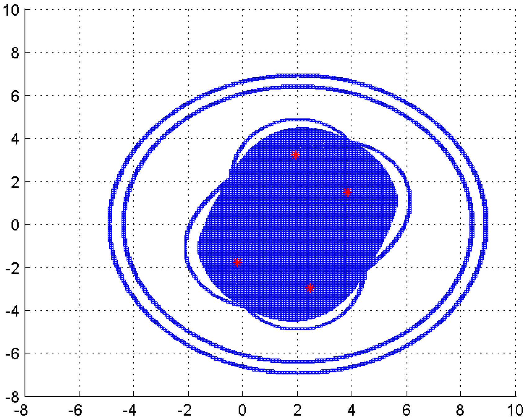
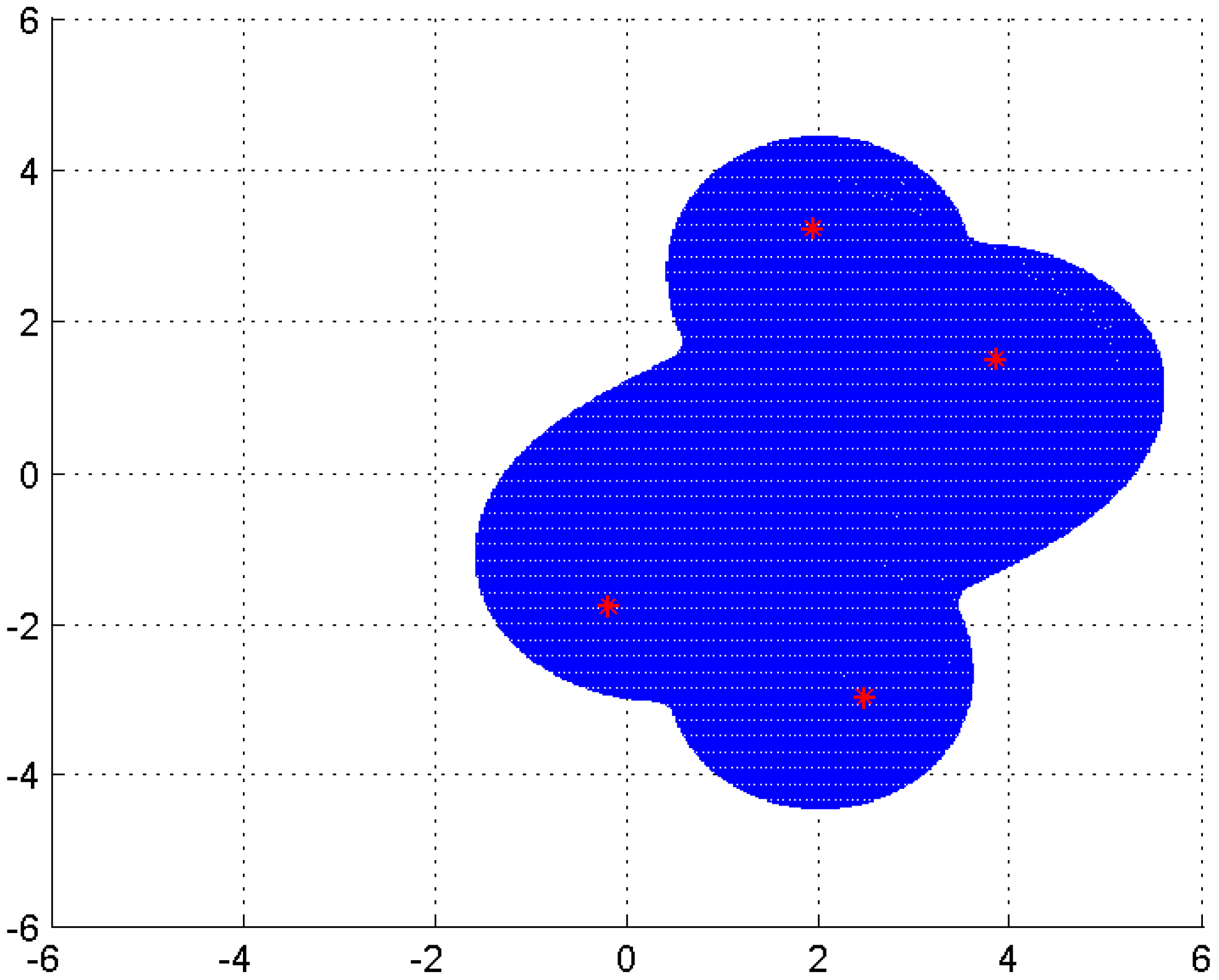
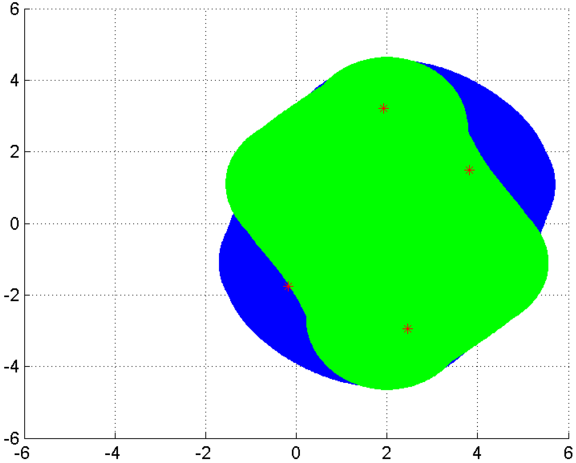
Example 1.

Consider the matrix A (the matrix $A_4$ in [9]),

$$A=\left[\begin{array}{cccc}2& i& -3& -i\\ 0& 2& 1& -5i\\ 4& 1& 2& 2\\ i& -1& 1& 2\end{array}\right].$$

the sets $\Gamma \left(A\right)$, $\mathcal{K}\left(A\right)$, $\Omega \left(A\right)$, and $\overline{\Omega }\left(A\right)$ are shown in Figure 1, where $\Gamma \left(A\right)$ is represented by the outside boundary, $\mathcal{K}\left(A\right)$ by the middle, $\Omega \left(A\right)$ by the inner, and $\overline{\Omega }\left(A\right)$ is filled. The exact eigenvalues are plotted with asterisks. It is easy to see that

$$\overline{\Omega }\left(A\right)\subset \Omega \left(A\right)\subset \mathcal{K}\left(A\right)\subset \Gamma \left(A\right).$$

This example shows that the the new eigenvalue inclusion set in Theorem 4 is tighter than the Geršgorin set $\Gamma \left(A\right)$, the Brauer set $\mathcal{K}\left(A\right)$ and the set $\Omega \left(A\right)$ obtained in [9].

Remark 1.

From Theorems 3 and 5, we have that

$$\overline{\Omega }\left(A\right)\subseteq \Omega \left(A\right),\overline{\Omega }\left(A^T\right)\subseteq \Omega \left(A^T\right),\left(\overline{\Omega }\left(A\right)\bigcap \overline{\Omega }\left(A^T\right)\right)\subseteq \left(\Omega \left(A\right)\bigcap \Omega \left(A^T\right)\right)$$

and

$${\Omega }^2\left(A\right)\subseteq {\Omega }^1\left(A\right)\subseteq (\Omega \left(A\right)\bigcap \Omega \left(A^T\right)).$$

Note here that ${\Omega }^1\left(A\right)={\Omega }^1\left(A^T\right)$ and ${\Omega }^2\left(A\right)={\Omega }^2\left(A^T\right)$. However, the sets ${\Omega }^2\left(A\right)$ and $\overline{\Omega }\left(A\right)\bigcap \overline{\Omega }\left(A^T\right)$ (also ${\Omega }^1\left(A\right)$ and $\overline{\Omega }\left(A\right)\bigcap \overline{\Omega }\left(A^T\right)$) cannot be compared with each other. In fact, we also consider the matrix A in Example 1, and draw ${\Omega }^2\left(A\right)$, and $\overline{\Omega }\left(A\right)\bigcap \overline{\Omega }\left(A^T\right)$ in Figure 2 and Figure 3. It is not difficult to see that

$${\Omega }^2\left(A\right)\subseteq /\overline{\Omega }\left(A\right)\bigcap \overline{\Omega }\left(A^T\right)$$

and

$$\overline{\Omega }\left(A\right)\bigcap \overline{\Omega }\left(A^T\right)\subseteq /{\Omega }^2\left(A\right).$$

3. Eigenvalue Inclusion Set for Toeplitz Matrices

Toeplitz matrices, a subclass of matrices with a c.m.d., arise in many fields of application [12,13,14,15,16,17,18], such as probability and statistics, signal processing, differential and integral equations, Markov chains, Padé approximation, etc. For example, consider an assigned Lebesgue integrable function f defined on the fundamental interval $I=[-\pi ,\pi )$ and periodically extended to the whole real axis, and the Fourier coefficients $a_k$ of f that is

$$a_k=\frac{1}{2\pi }{\int }_{-\pi }^{\pi }f\left(x\right)e^{-\mathbf{i}kx}dx,({\mathbf{i}}^2=-1)$$

where k is an integer number. From the coefficients $a_k$ one can build the infinite dimensional Toeplitz matrix $Tn\left(f\right)$ with entries ${\left(Tn\left(f\right)\right)}_{st}=a_{s-t},s,t=1,2\dots ,n$ [12,13,16].

Toeplitz matrices are constant along all their NW-SE diagonals [7,9], i.e., a Toeplitz matrix $T\in {\mathbb{C}}^{n\times n}$ has the following form:

$$T=\left[\begin{array}{ccccc}{t}_0& t_1& t_2& \cdots & t_{n-1}\\ t_{-1}& t_0& t_1& \cdots & t_{n-2}\\ ⋮& \ddots & \ddots & \ddots & ⋮\\ t_{2-n}& \cdots & t_{-1}& t_0& t_1\\ t_{1-n}& \cdots & t_{-2}& t_{-1}& t_0\end{array}\right].$$

Indeed, if f is a real valued function, we have $a_k={\overline{a}}_{-k}$ and, consequently, $T_n\left(f\right)$ is Hermitian; moreover, if $f\left(x\right)=f(-x)$, then the coefficients $a_k$ are real and $T_n\left(f\right)$ is symmetric. The following result can be found in [12,19] and in a multilevel setting in [16,17].

Theorem 6

([17,19]).Let ${\lambda }_j^{\left(n\right)}$ be the eigenvalues of $T_n\left(f\right)$ sorted in nondecreasing order, and $m_f=$ ess inf $f$, $M_f=$ ess sup $f$.

a. 

If $m_f<M_f$, then ${\lambda }_j^{\left(n\right)}\in (m_f,M_f)$ for every j and n; if $m_f=M_f$, then f is constant and trivially $T_n\left(f\right)=m_f{I}_n$ with $I_n$ identity of size n;

b. 

The following asymptotic relationships hold: ${\displaystyle \underset{n\to \infty }{lim}{\lambda }_1^{\left(n\right)}=m_f}$, ${\displaystyle \underset{n\to \infty }{lim}{\lambda }_n^{\left(n\right)}=M_f}$.

Furthermore, there exist further results establishing precisely how fast the convergence holds [13,17]. Since in applications (differential and fractional operators/equations, shift-invariant integral operators/equations, signal and image processing etc.) often the underlying Toeplitz matrices have large size n, then the results in [12,13,16,17] are difficult to beat and improved. When f is complex-values the theory is more complicated and in that case the convex hull of the essential range of f plays a role (see [13,18]). Obviously, a Toeplitz matrix is persymmetric. Here, we call A persymmetric if A is symmetric with respect to the main anti-diagonal [9]. Furthermore, the square of a Toeplitz matrix T is not necessary Toeplitz, but it is persymmetric.

In [9], Melman applied the eigenvalue inclusion Theorem (Theorem 1) of matrices with a c.m.d. to Toeplitz matrices, and obtained the following simpler form of the eigenvalue inclusion set.

Theorem 7 

([9] Theorem 3.1).Let $T=\left[t_{ij}\right]\in {\mathbb{C}}^{n\times n}$ be a Toeplitz matrix and $t_{ii}=\overline{t},n\ge 2$. Then,

$$\sigma \left(T\right)\subseteq \Omega \left(T\right)=\bigcup _{i=1}^{\lceil \frac{n}{2}\rceil }{\Omega }_i\left(T\right),$$

where

$${\Omega }_i\left(T\right)=\{z\in \mathbb{C}:|z-\overline{t}-\sqrt{{\left(T_0^2\right)}_{ii}}\left|\right|z-\overline{t}+\sqrt{{\left(T_0^2\right)}_{jj}}|\le v_i\left(T_0^2\right)\},$$

$$T_0=T-\overline{t}I,v_i\left(T_0^2\right)=max\{r_i\left(T_0^2\right),r_{n-i+1}\left(T_0^2\right)\},$$

and

$$\lceil \frac{n}{2}\rceil =\left\{\begin{array}{cc}\frac{n}{2},& ifniseven,\\ \frac{n+1}{2},& ifnisodd.\end{array}\right.$$

Furthermore, $\Omega \left(T\right)\subseteq \mathcal{K}\left(T\right)\subseteq \Gamma \left(T\right)$.

Next, by applying Theorem 4 to Toeplitz matrices, we obtain a new eigenvalue inclusion set.

Theorem 8.

Let $T=\left[t_{ij}\right]\in {\mathbb{C}}^{n\times n}$ be a Toeplitz matrix with $t_{11}=\overline{t}$ and $n\ge 2$. Then,

$$\sigma \left(T\right)\subseteq \overline{\Omega }\left(T\right)=\left(\bigcup _{i,j\in \lceil \frac{n}{2}\rceil ,i\ne j}{\overline{\Omega }}_{ij}^1\left(T\right)\right)\bigcup \left(\bigcup _{i\in \lceil \frac{n}{2}\rceil }{\overline{\Omega }}_i\left(T\right)\right),$$

where

$$\begin{array}{cc}\hfill {\overline{\Omega }}_{ij}^1\left(T\right)=\{z\in \mathbb{C}:& |z-t_0-\sqrt{{\left(T_0^2\right)}_{ii}}\left|\right|z-t_0+\sqrt{{\left(T_0^2\right)}_{ii}}|\\ & |z-t_0-\sqrt{{\left(T_0^2\right)}_{jj}}\left|\right|z-t_0+\sqrt{{\left(T_0^2\right)}_{jj}}|\le V_i\left(T_0^2\right)V_j\left(T_0^2\right)\},\end{array}$$

$${\overline{\Omega }}_i\left(T\right)=\{z\in \mathbb{C}:{\left(|z-t_0-\sqrt{{\left(T_0^2\right)}_{ii}}\left|\right|z-t_0+\sqrt{{\left(T_0^2\right)}_{ii}}|\right)}^2\le r_i\left(T_0^2\right)r_{n-i+1}\left(T_0^2\right)\},$$

$$V_i\left(T_0^2\right)=max\{r_i\left(T_0^2\right),r_{n-i+1}\left(T_0^2\right)\},and{T}_0=T-t_{0}I.$$

Proof. 

Since T is Toeplitz and $T_0=T-\overline{t}I$, we have that $T_0$ is also Toeplitz and $T_0^2$ is persymmetric. Therefore, the main diagonal of $T_0^2$ has at most $\lceil \frac{n}{2}\rceil$ distinct values, and ${\left(T_0^2\right)}_{ii}={\left(T_0^2\right)}_{n-i+1,n-i+1}$ for $i=1,2,\dots ,\lceil \frac{n}{2}\rceil$. Hence, by Theorem 4 and Equation (6), for any $\lambda \in \sigma \left(T\right),$ $\lambda \in \overline{\Omega }\left(T\right)=\bigcup _{i,j\in N,i\ne j}{\overline{\Omega }}_{ij}\left(T\right)$. For the case $i,j\in \{1,2,\dots ,\lceil \frac{n}{2}\rceil \},j\ne i$, we have

$$|{(\lambda -\overline{t})}^2-{\left(T_0^2\right)}_{ii}\left|\right|{(\lambda -\overline{t})}^2-{\left(T_0^2\right)}_{jj}|\le r_i\left(T_0^2\right)r_j\left(T_0^2\right).$$

(10)

For the case $i\in \{1,2,\dots ,\lceil \frac{n}{2}\rceil \}$, $j\in N\setminus \{1,2,\dots ,\lceil \frac{n}{2}\rceil \}$, $j\ne n-i+1$, we have

$$|{(\lambda -\overline{t})}^2-{\left(T_0^2\right)}_{ii}\left|\right|{(\lambda -\overline{t})}^2-{\left(T_0^2\right)}_{n-j+1,n-j+1}|\le r_i\left(T_0^2\right)r_{n-j+1}\left(T_0^2\right).$$

Note that ${\left(T_0^2\right)}_{jj}={\left(T_0^2\right)}_{n-j+1,n-j+1}$, then

$$|{(\lambda -\overline{t})}^2-{\left(T_0^2\right)}_{ii}\left|\right|{(\lambda -\overline{t})}^2-{\left(T_0^2\right)}_{jj}|\le r_i\left(T_0^2\right)r_{n-j+1}\left(T_0^2\right).$$

(11)

From Inequalities (10) and (11), we can get that

$$|{(\lambda -\overline{t})}^2-{\left(T_0^2\right)}_{ii}\left|\right|{(\lambda -\overline{t})}^2-{\left(T_0^2\right)}_{jj}|\le r_i\left(T_0^2\right)V_j\left(T_0^2\right),$$

(12)

where $V_j\left(T_0^2\right)=max\{r_j\left(T_0^2\right),r_{n-j+1}\left(T_0^2\right)\}.$ Similarly, we obtain

$$|{(\lambda -\overline{t})}^2-{\left(T_0^2\right)}_{n-i+1,n-i+1}\left|\right|{(\lambda -\overline{t})}^2-{\left(T_0^2\right)}_{jj}|\le r_{n-i+1,n-i+1}\left(T_0^2\right)V_j\left(T_0^2\right).$$

(13)

From ${\left(T_0^2\right)}_{ii}={\left(T_0^2\right)}_{n-i+1,n-i+1}$, Inequalities (12) and (13), we could easily get, for any $i,j\in \{1,2,\dots ,\lceil \frac{n}{2}\rceil \}$ and $j\ne i$,

$$|{(\lambda -\overline{t})}^2-{\left(T_0^2\right)}_{ii}\left|\right|{(\lambda -\overline{t})}^2-{\left(T_0^2\right)}_{jj}|\le V_i\left(T_0^2\right)V_j\left(T_0^2\right).$$

(14)

Furthermore, for any $i\in \{1,2,\dots ,\lceil \frac{n}{2}\rceil \},j=n-i+1,$

$$|{(\lambda -\overline{t})}^2-{\left(T_0^2\right)}_{ii}\left|\right|{(\lambda -\overline{t})}^2-{\left(T_0^2\right)}_{n-i+1,n-i+1}|\le r_i\left(T_0^2\right)r_{n-i+1}\left(T_0^2\right)$$

which is equivalent to

$$|{(\lambda -\overline{t})}^2-{\left(T_0^2\right)}_{ii}\left|\right|{(\lambda -\overline{t})}^2-{\left(T_0^2\right)}_{i,i}|\le r_i\left(T_0^2\right)r_{n-i+1}\left(T_0^2\right),$$

that is,

$${\left(|z-t_0-\sqrt{{\left(T_0^2\right)}_{ii}}\left|\right|z-t_0+\sqrt{{\left(T_0^2\right)}_{ii}}|\right)}^2\le r_i\left(T_0^2\right)r_{n-i+1}\left(T_0^2\right).$$

(15)

The conclusion follows from Inequalities (14) and (15).  ☐

From Theorems 5, 7 and 8, we can obtain easily the comparison results as follows.

Theorem 9.

Let $T=\left[t_{ij}\right]\in {\mathbb{C}}^{n\times n}$ be a Toeplitz matrix with $t_{11}=\overline{t}$ and $n\ge 2$. Then,

$$\overline{\Omega }\left(T\right)\subseteq \Omega \left(T\right)\subseteq \mathcal{K}\left(T\right)\subseteq \Gamma \left(T\right).$$

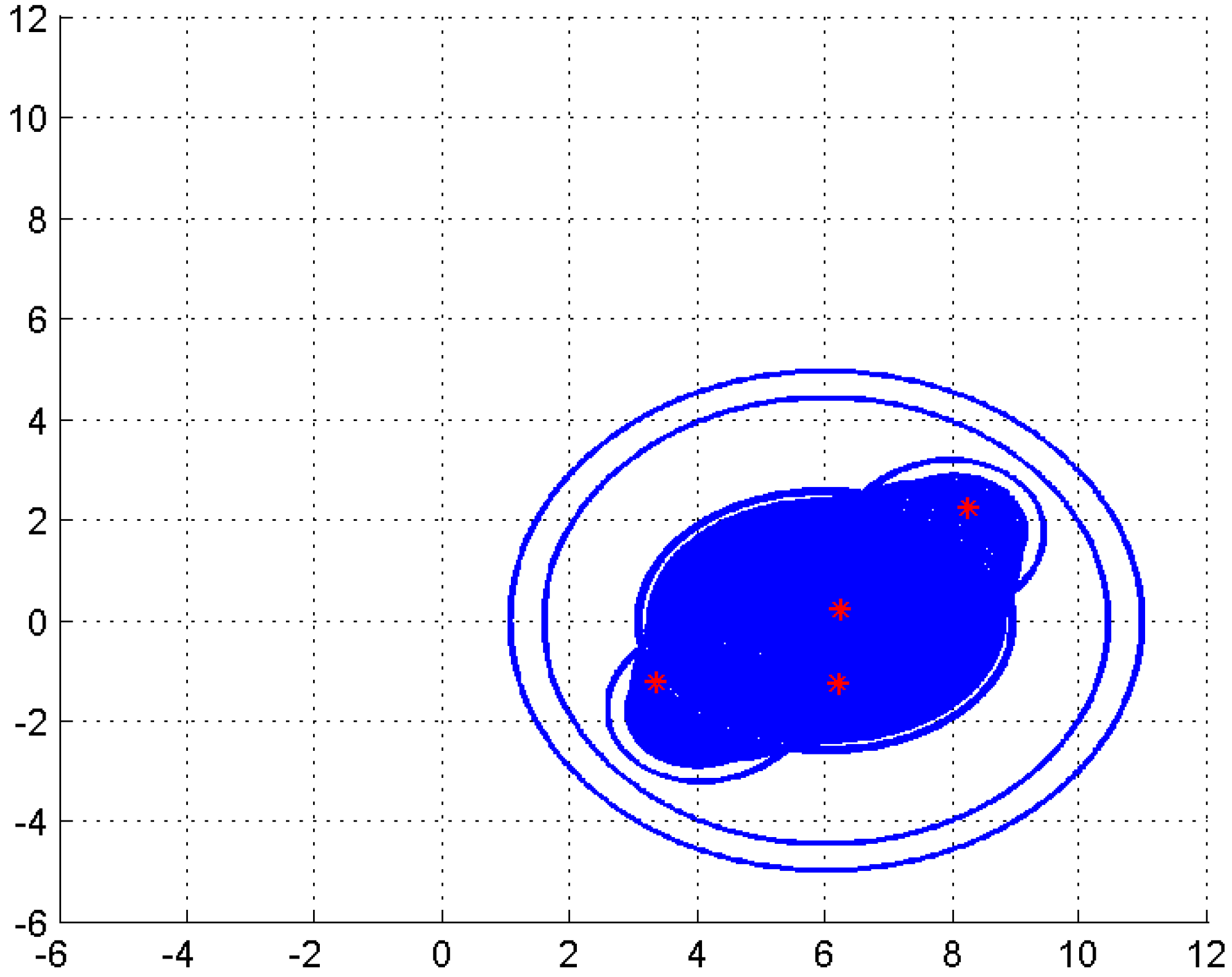
Example 2.

Consider the Toeplitz matrix Q in [9]:

$$Q=\left[\begin{array}{cccc}6& 1& -1& -2i\\ 0& 6& 1& -1\\ -1& 0& 6& 1\\ 4& -1& 0& 6\end{array}\right].$$

In Figure 4, the sets $\Gamma \left(Q\right)$, $\mathcal{K}\left(Q\right)$, $\Omega \left(Q\right)$, and $\overline{\Omega }\left(Q\right)$ are shown, where $\Gamma \left(Q\right)$ is represented by the outside boundary, $\mathcal{K}\left(Q\right)$ by the middle, $\Omega \left(Q\right)$ by the inner, and $\overline{\Omega }\left(Q\right)$ is filled. The exact eigenvalues are plotted with asterisks. As we can see,

$$\overline{\Omega }\left(Q\right)\subset \Omega \left(Q\right)\subset \mathcal{K}\left(Q\right)\subset \Gamma \left(Q\right).$$

This example shows that the new eigenvalue inclusion set in Theorem 8 is tighter than the set obtained in [9], the Geršgorin set and the Brauer set for a Toeplitz matrix.

4. Conclusions

In this paper, we obtain a new eigenvalue inclusion set for matrices with a c.m.d. We then apply this result to Toeplitz matrices, and get a set including all eigenvalues of Toeplitz matrices. Although they needs more computations to obtain the new eigenvalue sets than those in [9], the new sets capture all eigenvalues more precisely than those in [9].

References

- Brauer, A. Limits for the characteristic roots of a matrix II. Duke Math. J. 1947, 14, 21–26. [Google Scholar] [CrossRef]
- Cvetković, L. H-matrix theory vs. eigenvalue localization. Numer. Algorithms 2006, 42, 229–245. [Google Scholar] [CrossRef]
- Cvetković, L.; Kostić, V.; Bru, R.; Pedroche, F. A simple generalization of Geršgorin’s theorem. Adv. Comput. Math. 2011, 35, 271–280. [Google Scholar] [CrossRef]
- Cvetković, L.; Kostić, V.; Varga, R.S. A new Geršgorin-type eigenvalue inclusion set. Electron. Trans. Numer. Anal. 2004, 18, 73–80. [Google Scholar]
- Geršgorin, S. U¨ber die Abgrenzung der Eigenwerte einer Matrix. Izv. Akad. Nauk SSSR Ser. Mat. 1931, 1, 749–754. [Google Scholar]
- Li, C.Q.; Li, Y.T. Generalizations of Brauer’s eigenvalue localization theorem. Electron. J. Linear Algebra 2011, 22, 1168–1178. [Google Scholar] [CrossRef]
- Li, C.Q.; Li, Y.T. New regions including eigenvalues of Toeplitz matrices. Linear Multilinear Algebra 2014, 62, 229–241. [Google Scholar] [CrossRef]
- Melman, A. Modified Gershgorin Disks for Companion Matrices. Siam Rev. 2012, 54, 355–373. [Google Scholar] [Green Version]
- Melman, A. Ovals of Cassini for Toeplitz matrices. Linear Multilinear Algebra 2012, 60, 189–199. [Google Scholar] [CrossRef]
- Sang, C.L.; Zhao, J.X. Eventually DSDD Matrices and Eigenvalue Localization. Symmetry 2018, 10, 448. [Google Scholar] [CrossRef]
- Varga, R.S. Geršgorin and His Circles; Springer: Berlin, Germany, 2004. [Google Scholar]
- Di Benedetto, F.; Fiorentino, G.; Serra, S. CG preconditioning for Toeplitz matrices. Comput. Math. Appl. 1993, 25, 35–45. [Google Scholar] [CrossRef]
- B¨ttcher, A.; Grudsky, S. On the condition numbers of large semi-definite Toeplitz matrices. Linear Algebra Appl. 1998, 279, 285–301. [Google Scholar] [CrossRef]
- Bunch, J.R. Stability of methods for solving Toeplitz systems of equations. SIAM J. Sci. Stat. Comput. 1985, 6, 349–364. [Google Scholar] [CrossRef]
- Pourahmadi, M. Remarks on extreme eigenvalues of Toeplitz matrices. Int. J. Math. Math. Sci. 1988, 11, 23–26. [Google Scholar] [CrossRef] [Green Version]
- Serra, S. Preconditioning strategies for asymptotically ill-conditioned block Toeplitz systems. BIT 1994, 34, 579–594. [Google Scholar] [CrossRef]
- Serra, S. On the Extreme Eigenvalues of Hermitian (Block) Toeplitz Matrices. Linear Algebra Appl. 1998, 270, 109–129. [Google Scholar] [CrossRef]
- Capizzano, S.S.; Tilli, P. Extreme singular values and eigenvalues of non-Hermitian block Toeplitz matrices. J. Comput. Appl. Math. 1999, 108, 113–130. [Google Scholar] [CrossRef]
- Grenander, U.; Szego¨, G. Toeplitz Forms and Their Applications, 2nd ed.; Chelsea: New York, NY, USA, 1984. [Google Scholar]
Figure 1.
.
Figure 2.
Figure 3.
Figure 4.
© 2018 by the authors. Licensee MDPI, Basel, Switzerland. This article is an open access article distributed under the terms and conditions of the Creative Commons Attribution (CC BY) license (http://creativecommons.org/licenses/by/4.0/).
Share and Cite
MDPI and ACS Style
Zhang, W.; Li, C. An Eigenvalue Inclusion Set for Matrices with a Constant Main Diagonal Entry. Symmetry 2018, 10, 745. https://0-doi-org.brum.beds.ac.uk/10.3390/sym10120745
AMA Style
Zhang W, Li C. An Eigenvalue Inclusion Set for Matrices with a Constant Main Diagonal Entry. Symmetry. 2018; 10(12):745. https://0-doi-org.brum.beds.ac.uk/10.3390/sym10120745
Chicago/Turabian StyleZhang, Weiqian, and Chaoqian Li. 2018. "An Eigenvalue Inclusion Set for Matrices with a Constant Main Diagonal Entry" Symmetry 10, no. 12: 745. https://0-doi-org.brum.beds.ac.uk/10.3390/sym10120745
Note that from the first issue of 2016, this journal uses article numbers instead of page numbers. See further details here.