PV Forecasting Using Support Vector Machine Learning in a Big Data Analytics Context


1
Oracle Romania, Floreasca Park 43 Soseaua Pipera, Bucharest 014254, Romania
2
Department of Economic Informatics and Cybernetics, The Bucharest University of Economic Studies, Romana Square 6, Bucharest 010374, Romania
*
Author to whom correspondence should be addressed.
Symmetry 2018, 10(12), 748; https://0-doi-org.brum.beds.ac.uk/10.3390/sym10120748
Submission received: 12 November 2018
/
Revised: 8 December 2018
/
Accepted: 11 December 2018
/
Published: 13 December 2018
Abstract
:Renewable energy systems (RES) are reliable by nature; the sun and wind are theoretically endless resources. From the beginnings of the power systems, the concern was to know “how much” energy will be generated. Initially, there were voltmeters and power meters; nowadays, there are much more advanced solar controllers, with small displays and built-in modules that handle big data. Usually, large photovoltaic (PV)-battery systems have sophisticated energy management strategies in order to operate unattended. By adding the information collected by sensors managed with powerful technologies such as big data and analytics, the system is able to efficiently react to environmental factors and respond to consumers’ requirements in real time. According to the weather parameters, the output of PV could be symmetric, supplying an asymmetric electricity demand. Thus, a smart adaptive switching module that includes a forecasting component is proposed to improve the symmetry between the PV output and daily load curve. A scaling approach for smaller off-grid systems that provides an accurate forecast of the PV output based on data collected from sensors is developed. The proposed methodology is based on sensor implementation in RES operation and big data technologies are considered for data processing and analytics. In this respect, we analyze data captured from loggers and forecast the PV output with Support Vector Machine (SVM) and linear regression, finding that Root Mean Square Error (RMSE) for prediction is considerably improved when using more parameters in the machine learning process.
1. Introduction
Due to the constantly increasing need for energy in the last decade and climate change issues, RES are vital. However, any electric power generation system needs to balance the generating and the loading components in order to be reliable and to operate safely at quality standards in terms of voltage, frequency and stability regulation [1]. This is also available for smaller scale systems such as prosumers, communities, aggregators or micro-grids that deal with local generation and consumption. Unfortunately, both the generating and loading components have fluctuations. RES, in comparison with other energy resources, do not fail unexpectedly, but they are characterized by uncertainty and variability. To compensate for these issues, other power system reserves are involved to generate additional power or reduce power when needed.
When monitoring RES, the main target is to identify whether the system is running in optimum conditions [2] or not. For monitoring, we need to measure some parameters and determine the RES yield. One of the common approaches for generating the forecast is to collect historical data, define the prediction problem, develop a forecasting model, validate and apply it and give meaning to the results. Collecting data from sensors is very time-consuming, but it is also one of the most significant processes [3], as it tremendously influences the forecast accuracy. Another approach is to measure some typical parameters that are used in generating graphs; these are subsequently compared over a period of time or with a reference in order to determine whether RES are running properly [2] or if deviations can be identified. Some of the main activities in this process are the measuring and storing of parameters that in some scenarios can generate a huge volume of data.
A monitoring system consists of a data acquisition component based on sensors and an analytical component that processes a specific set of parameters by recording, storing, mining and performing statistical and big data analytical activities.
In [4], it is mentioned that the collected data can be used for the determining of the grid stability. By analogy, this data also provides information about the off-grid or hybrid RES stability and about the power quality (the level of power disturbances and harmonics, which should be as small as possible). On the same level, one of the most important tasks of the monitoring activity is to determine, in advance, a possible grid failure or RES failure (outages of the system due to component failures), and then to notify the operator and provide the opportunity to replace the necessary power using alternative sources.
Forecasting RES generation is essential since an accurate forecast ensures better grid integration as fluctuations can be overcome and thus not represent a barrier anymore. Wind and solar power producers can gain additional benefits from the forecast, considering that maintenance can be scheduled for when the wind speed and solar irradiance are low or the electricity price on the market is suitable.
The producers of renewable energy have an increasing interest in forecasting the loading process. Analytics and big data can help with processing large amounts of historical data, thus increasing the wind, solar and loading forecast accuracy. Also, based on data mining, it is possible to perform customer profiling, which is helpful for the loading prediction and for the functionality optimization of critical parts of the system like inverters or storage battery bank. Using historical consumption data and social and economic indicators, it is possible to accurately forecast the load for long periods [5].
Lately, it has become widely accepted that climate change has visible effects that are quantified as increased funding allocated to renewable items [6]. Renewable energy technologies have a broad range of variability that raises challenges in terms of the electricity grid. They exist for both off-grid and on-grid systems.
In some bibliographic sources, small RES are known as micro-grids [7] that combine energy capabilities, storage, advanced technologies that use sensors and actuators, IT&C, big data, complex analytics, etc.
The purpose of our paper is to underline the implication of sensors and loggers in collecting and manipulating data for RES, in the context of promoting the usage of big data and analytics. We structured the paper in seven sections. In the current section, a short introduction related to RES, especially PV, is provided. The second section gives an overview of related works regarding RES, data extracted from sensors and PV forecast. The methodology is presented in Section 3, which focuses on sensor data and analytics in the context of the PV forecasting with the support vector machine (SVM). A brief estimation of the quantity of data generated by loggers in some practical RES cases is also provided. Section 4 consists of a sample usage of a data logger that provides six examples of PV forecasting using SVM. In the discussion section, some opinions, deduced from previous sections and from simulations or comparisons with other sources, are given. Then, we emphasized the challenges related to data integration from sensors, loggers, big data and analytics. The conclusions are synthesized in the last section.
2. Literature Review
In [8], the authors present an example of optimization for an irrigation system that uses photovoltaic systems. It is optimized based on a fuzzy method that uses analytics and big data. Considering the very promising results, the solution could be extended to a larger scale.
The forecasted PV power [9] is mainly based on data available from PV and weather conditions using a learning machine (such as the Support Vector Regression). When there are many distribution companies, it is recommended to perform forecasting at the region level, thus considerably improving the estimation accuracy.
In [10], the authors describe how power output is optimized for a smart house with PV panels. The energy flow is managed based on the PV power forecasts, which use data from weather simulations, weather observations, component characteristics (modules, inverters). Also, it uses PV data obtained from monitoring. In this research, the electricity cost over a period of three days is minimized; the main focus is on the battery storage charge process and the hot water storage (another form of energy storage).
In [11], the energy management is described via a dynamic perspective using the loading process and the data forecasting. It is worth mentioning that the following models have been used: regression, linear and nonlinear time series, and state-space. It must also be underlined that the data collected from the sensors should be of good quality and reliable, as they are a significant factor for the optimization of the photovoltaic and wind energy systems.
The smart grid has become more and more common as a paradigm [12]. If the system is hybrid or on-grid, then renewable energy forecasting is often required, which means that the importance of sensors and loggers will increase in the near future. Short- and long-term PV forecasting is approached in many sources, such as [13,14,15]. In [12], the authors present a solar forecast survey. The study shows that there are many initiatives in this field, and that for many companies (around 50%), the cost of forecasting is still high.
The importance of monitoring wind turbines and the diversity of sensors that exist for the wind turbines are described in [16]. The existence of many sensors is mentioned and they can be categorized as follows: sensors that monitor the turbine output power, the temperature in the gearbox (oil temperature), the wind speed sensor, the nacelle temperature, the wind generator temperature, the acoustic sensors for determining the frequency of various vibrations (tower, blades). The data from these sensors are transmitted to a central node, named the control unit, where, based on data processing, the status of each turbine is monitored.
In the case of modern wind turbines with higher capacity, due to the high volume of blades, if imbalances in blade load exist, they can generate premature turbine frazzle. To overcome this, a load root sensor on each blade is used [17]. This sensor provides information to a system that will reduce the unbalanced turbine blade loads using pitch actuators.
An interesting discussion about sensors in RES is given in [18], where a particularity of the use of autonomous sensors for the wind system is described. An important aspect seems to be the wind system stretching autonomous function.
In [19], different methods for the photovoltaic array optimization are presented, such as: the good load matching method, the battery storage method, the solar concentration and the sun-tracking method. Of these methods, the last one is easiest to implement and is based on sun sensors. The sun sensors provide information about the relative position of the sun. This is primary information for the tracking system, which usually assures more energy for harvesting, with about 30% more than a system that has no tracking mechanism.
Recently, due to global warming, two new challenges have arisen: renewable energy resources management and environmental protection [20]. The estimation of the electrical power needed for an entity represents the load forecasting [21]. Small and medium companies generate sustainable energy for their own consumption or market transactions. There are cases when we have a mixture: the energy produced is primarily used for own consumption and the excess goes to the grid. The Load Forecasting from the Grid perspective (LFG) is discussed in [5,21,22,23]. The Load Forecasting for Own consumption or mixture (LFO) could have been similarly approached but, in our opinion, has many particularities that are referred to in the next paragraph. First of all, LFO is little discussed in the literature. LFO is necessary for fulfilling a balance between supply and demand (or, more particularly, between generation and consumption). However, if LFG is mainly necessary for balance, LFO is not always as critical, even if there is no balance. Most companies are connected to the public grid and can consume energy from it. However, LFO can be tremendously significant in the case of RES optimization.
LFG depends on many macroeconomic features (GDP, the industrial production, the number of households, population, etc.) [21]. By comparison, LFO depends less on these features, because LFO is referring to a smaller entity. Even in this case, the load forecasting is a complex task because it generally depends on several factors, such as: time (hour or even minute from day), week, month, season; weather conditions (temperature, wind, cloud cover, visibility, humidity, pressure, ceiling, etc.); social and political events, activities, work schedule, social media, income, energy price, etc.; assumptions about business development, and number of employees.
Even if LFO is implemented at a smaller scale, using big data is challenging for collecting and discovering relevant information for the load forecasting, due to the many dependent factors.
Based on the forecast time horizon, there are three types of load forecasting [21]: short-term—up to 24 h, medium-term—days or weeks, and long-term—months or years. For the short-term load forecasting [24], the artificial neural network (ANN) is recommended for both LFG and LFO. Based on [21,24], other recommended approaches are: regression, the fuzzy method, and the Box–Jenkins method.
In [24], there is mention of a very concise short-term forecasting purpose for the operational task that is a valid case for both LFG and LFO. Other forecasting methods [15] for the solar energy estimation of short time horizon are the time series with ANN nonlinear autoregressive (NAR) or the exogenous inputs nonlinear autoregressive (NARX).
RES can benefit from huge amounts of data [8] that come from smart meters, sensor networks, credit histories, customer payment information, logs from applications, machine logs, web servers’ logs, and satellite imagery. Also, other sources like social media, public web, media, archives, data sources and documents can be investigated. These data may play an important role when used as big data, which, through advanced analytics, can harness the energy market potential and provide possible clues about areas where energy access should be expanded or areas where the energy demand will substantially increase. For sustainable energy [8], there has been created a database [25] that has free data in order to support analyses in this field.
Both in the case of load forecasting and generation forecasting, data mining plays an important role because large amounts of data are available for making predictions. The main factors that recommend big data in the load forecasting [26] are the already available time series regarding data from different businesses and parameters generated by RES. The existence of time series generated in the last 15 years adds value to data mining and big data analytics. In the context of big data, the selection process can be a little more challenging due to the huge number of variables [26]. However, this cannot be too problematic since specific big data technologies, such as MapReduce, have been deployed in data analysis.
Usually, the data collected from sensors are in the form of a continuous flow or stream, sometimes of different formats, sizes and variability. For this reason, most analytical activities are done in real time or continuously [11] and only the results of real-time analytics or a part of sensor data are stored in relational or NoSQL databases. These particularities of data extracted from the sensors are leading to using big data and afferent technologies like artificial intelligence, machine learning, distributed computing, data analytics and data warehousing.
In the past, in order to work with a high volume of datasets, the solution was to scale up the hardware. Once big data technologies evolved, especially parallel processing and distributed architecture, the machine learning algorithms were transformed or adapted in order to benefit from new features [27]. They allow the use of specially designated scale-out storage space to apply machine learning algorithms to huge data volumes.
When the utility companies begin to use smart grid platforms, the collected datasets are not used to their full value [28] for various reasons such as: inappropriate infrastructure (hardware, network, applications, and storage space), inappropriate data science employee skills, etc. This problem usually appears because the utility companies are not initially aware of the full complexity of big data, thus losing the opportunity to control the forecast, the loading process, the prices and the monitoring objectives. With regard to the RES that work offline or in hybrid mode, the same issue can appear when all the existing information is not used. In the case of these energy producers, there can be smaller datasets and the big data processing resources are limited.
The data collected in the case of RES can be standard or continuous. Some data come in the form of continuous streams from sensors; other types of data can be standard, which means they are not changing rapidly in time. Therefore, the analytical software requires the capacity to analyze both data that change fast, by using an interactive approach, and data that are static, by using batch processing.
In [29], the forecast in the context of microgrids is mentioned. We consider that they also have a decentralized management (the decision is not too tightly bound to the grid). In this case, the forecast is highly dependent on the local approach, meaning that it needs to be based on the weather forecast and on the measurements and records of the monitoring RES system.
The PV energy forecast depends on the weather parameters and the PV panel characteristics [12]. Therefore, the PV energy forecasting methods are a mix, considering both the weather parameters and the PV panel characteristics. The sky imagery and the satellite imaginary methods, based on cloud images, are often used when images are available. The sky imagery can better predict for short time periods (30 min), while the satellite imaging prediction can be suitable for the upcoming hours (5–6 h) [12]. To increase the accuracy of the PV energy forecasting [12], it is recommended to combine the forecast models.
In smart grids, the data analytics is usually oriented to grid operations [28], meaning they are used for understanding customers’ behavior, the predictive load and the forecasted energy. For the off-grid and hybrid renewable energy systems, the analytics should be similar. The offline and hybrid RES of medium to large sizes that use sensors, analytics and big data processing can be called Smart Off-line Renewable Energy Systems (SORES) and Smart Hybrid Renewable Energy Systems (SHRES), respectively. SORES and SHRES are similar to the micro-grids that (partially) operate without public grid connection. Usually, grid connecting is desired, but for some reasons this may not be possible for isolated sites or as a result of the local legislation. Connecting to the grid implies some additional administrative tasks performed in the grid, which can be simplified by using big data and analytics. Similarly to micro-grids [30], SORES and SHRES [30] represent an easy way to use or integrate renewable energy in local communities by having reduced costs, good reliability and decreased CO2 emissions. These kinds of systems alleviate the grid’s difficult task of delivering energy where technical difficulties exist. When referring to the grid and RES, there are two main directions for generating wind and photovoltaic energy [7]. The first consists of encouraging and deploying large wind and photovoltaic power plants that can be smoothly integrated into the grid. The second direction has an opposite purpose: to have many small wind turbines and photovoltaic panels that require more decentralized action, in accordance with smart grids and smart cities. In order to successfully manage such complex systems, it is very useful to use big data and analytics, in the case of a decentralized approach.
An important aspect regarding big data in the energy field is data integration. Thus, the data collected by sensors, weather data, energy consumption and also GIS (Geographic Information System) data are tightly integrated. Basically, some specific big data analyses are not suitable without data integration—in particular, without GIS data integration [20].
Due to the progress of electronics and the cost-accessible sensors, the monitoring process goes a step further. In general, monitoring has been done at the inverter or solar controller level because here the data can be easily accessed. The implementation of the sensors for monitoring the photovoltaic panels is proposed in [31,32]. Such monitoring systems are usually modules that communicate wireless and contain a small number of cheaper sensors. A similar approach is suggested in [33] where the temperature is monitored for every panel using wired communication, which allows the monitoring of the generated power individually per PV panel [2]. The solution is accessible because the data transmission is cheaper via wire. Also, there is only one sensor and the data volume is not too large, which reduces the number of tasks at the big data analytical level.
In general, specific forecasting systems perform at their best depending on the forecasted time horizon. The numerical weather prediction models are recommended for short periods such as 1–2 days; the statistical models (ANN in special), eventually combined with image models (sky or satellite), are suitable for even shorter periods, under 6 h [12]. For RES systems, this last category is very useful because we can adjust it based on consumption. Using big data and analytics for the distributed generation is also useful for better integration into the grid of the small wind and the photovoltaic generators.
In [34], the authors propose monitoring the PV module by attaching it to the cover glass of an optical fiber sensor for measuring the temperature. This can be further extended to attaching this type of sensor at the photovoltaic cell level. In this manner, monitoring the PV panel becomes more accurate by having more data for analytics.
3. Methodology
The proposed methodology can be performed following these three steps: collecting and integrating data from sensors and smart meters, processing data with big data technologies, and forecasting PV and other RES outputs by SVM, as shown in Figure 1.
First, the weather data acquisition block is used for obtaining the weather data parameters. They can be achieved from a weather station using sensors or from a software application that uses a weather API. The inverters provide the following input parameters: power, current, voltage, etc. for each inverter or at the array level.
The data logger and/or the solar controller block measure the same parameters: power, current, voltage, etc. using a data logger that records and transmits them. Some solar controllers have the ability to provide the same function as independent data loggers.
The data transmission block assures the communication between the collected parameters and the storage and the processing block. The transmission can be made via wire (Ethernet LAN, WAN) or using wireless transmitting technologies, such as: Wi-Fi, Bluetooth, etc. The storage and the processing block can vary from flat files to databases or even big data.
The PV analytic forecast block consists of several methods for forecasting the produced power (for example, machine learning like multi regression, SVM or artificial intelligence). This can be developed using technologies like R, Python, C, Java, etc.
3.1. Sensor Data
Data from sensors and simulations can be used to estimate the viability of the RES project, monitor system parameters in real time, forecast, maintain, optimize and properly size the system (by generating and storing in order to balance the demand).
One of the challenges related to collecting data from sensors is the huge datasets that usually contains multi-dimensional records. For instance, records collected by a logger from a photovoltaic panel can contain about 28 parameters. To extract knowledge and information from such datasets, it is imperative to find groups of similar data records and analyze them using data clustering [35]. Finding clusters is an important data mining step. Since the dataset is huge, it is recommended to find clusters in a subset of dimensions, usually named subspace.
Also, for off-grid systems, it is necessary to determine the optimum size for the storage capacity that reliably provides energy, which can be predicted with data analytics. Wind and solar power generation can be predicted using data from sensors through data mining techniques.
However, the challenges regarding the sensors [36] are related to cost, technical limitations regarding connectivity, privacy, security, sharing and data analysis.
The sensors can be classified as follows:
- -
- Simple sensors mounted near the renewable energy sources, such as: solar light sensors, temperature, humidity or even video cameras;
- -
- Advanced sensors for on-site monitoring [37], where an embedded device, based on a microcontroller, is added to a photovoltaic panel to measure the voltage and the power. Arduino-related sensors are similarly implemented. In both cases, data can be collected via wireless or LAN technologies and sent to a server.
- -
- High integrated sensors that are recently offered by RES equipment producers (solar and wind) and generate special “loggers.” These devices are connected to solar controllers via the RS485 interface, retrieve on a custom time interval all the voltage and the power parameters and locally store them for a specific time period, three months or one month, depending on the storage capacity. An example of such a logger is EPEVER eLOG01 for EPEVER MPPT solar controllers. Other producers have similar loggers directly integrated in the solar controllers.
- -
- Wireless Sensor Networks (WSN) represent a small module, which contains sensors, microcontrollers and radio transceivers. All principles related to WSN apply to PV, wind turbine or RES [38,39,40,41]. They provide a central data storage, access control, transmission techniques, multichannel and optimal sensor locations, energy efficiency sensors and transmission criteria. In the case of RES, WSN can contain one or more sensors for temperature, solar radiation and wind speed. However, in order to reduce the costs, only the back-panel temperature sensors can be used for PV, and only the wind speed sensor can be used for the wind turbines. Based on these two sensors, the generated power can be predicted. Another particularity of RES is that a relatively high number of WSN modules are necessary (in comparison with the logger modules), especially because it is desirable to monitor every element. Thus, it generates a huge data volume. The data collection, the aggregation and the analysis are highly dependent on technology, with the recommendation being to use big data.
- -
- Monitoring units that contain sensors for PV temperature, ambient temperature, solar radiation and a main unit. These units collect primary data and send them to a web portal from where the data can be processed in a big data environment (for example, the SM2-MU main unit). This situation is mentioned in [42,43]: to analyze large volumes of data, SM2-MU connects to a web portal to send data. The portal can have, in the background, the possibility of analyzing data. By extrapolation, it is possible to write data using a customized code into a repository or even into a big data system, where big data analytical features can be used.
- -
- Standalone sensors such as the PV-100 PV monitoring package, which contains PV temperature, ambient temperature and solar radiation sensors, plus a radiation shield to prevent errors. PV-100 PV is working on an SMA cluster controller. It is a SMA company product mentioned here since it implements a distinct monitoring principle for monitoring the PV system. As described in [44], the SMA cluster controller is a central unit that works with many SMA inverters and sensors, such as the previously mentioned PV-100 PV. SMA cluster records data from inverters and sensors and assures the monitoring and the control of the PV plant. It can interact with a web portal that allows for large-scale integration. The SMA cluster controller consists of an intelligent part of monitoring that collects and transmits data for many applications, providing seamless sensor integration.
The measuring of temperature, humidity, wind, rainfall and other environment parameters can be done on site, using a private or public weather station. This is a more economical approach than having sensors on every panel, but also less accurate. The weather stations can periodically dump data into a .csv file, which facilitates more data processing with big data techniques.
Another approach for determining the environment parameters is to use a weather API in a software application [45] in order to retrieve meteorological data at a specific time frequency. The weather API can retrieve data based on locations. Also, the weather APIs are less accurate than the weather stations, because the software on API retrieves meteorological data from a neighboring public weather station, which usually is at a specific distance from the location where RES is installed. The weather API can give more parameters, which via big data processing can compensate for the accuracy issue. In the future, many applications, services, and infrastructure platforms that aim at energy saving, will be based on weather data, and thus the weather parameters will have a growing significance [20].
The ambient temperature sensor and/or PV panel temperature sensor can play an important role. Thus, the PV panel temperature is proportional not only to the ambient temperature, but also to the solar radiation received by the panel. One report [2] presents the graphical difference between the PV panel temperature and the ambient temperature. Comparing this difference with the reference yield (Yr) at a weekly level, for example, and drawing a regression line could provide significant insights into the monitoring system.
Short examples of the quantity of data generated by sensors are provided in the following paragraphs:
- A logger used with one solar charge controller that records at 15-min frequencies: in one day, it generates 132 records, each with 27 attributes, stored in a .csv file of 20 KB. In one month, it stores 3960 records into a .csv file of 620 KB.
- Loggers used on a PV RES rooftop of 3kW with an array of 10 PV panels, each one of 300 W. If we consider, for example, 10 micro-inverters, each with an MPPT solar controller, and 10 loggers: in one day, they generate 1320 records stored in a .csv file of 200 KB. In one month, it stores 39,600 records into a .csv file of 6200 MB.
- Loggers used on a PV RES rooftop of 12 kW with an array of 40 PV panels, each one of 300 W, 40 micro-inverters/MPPT solar controller and 40 loggers: in one day, they generate 5320 records, stored in a .csv file of 800 KB. In one month, it stores 15,840 records in a .csv file of 24,800 MB.
- Loggers used on a PV RES rooftop of 24 kW with an array of 80 PV panels, each one of 300 W, 80 micro-inverters/MPPT solar controller and 80 loggers: in one day, they generate 10,640 records, stored in a .csv file of 1600 KB. In one month, it stores 31,680 records in a .csv file of 49,600 MB.
- Loggers used on a 100 kW PV system within a RES. Multiplying by 4 the data from the previous sample, in one day, it generates 42,560 records, stored in a .csv file of 6400 KB. In one month, it stores 126,720 records in a .csv file of 198,400 MB.
- Loggers used on 1 MW PV system within RES. Multiplying by 10 the data from the previous sample, in one day, it generates 425,600 records, stored in a .csv file of 64 MB. In one month, it stores 1,267,200 records in a .csv file of 1,980,400 GB.
These data are related to PV parameters only. Similar data volume can appear in the case of the weather variables. Also, considering that the data from the loggers are recorded at 3-min frequencies, the volume of data from the above examples is 5 times larger.
The data collected from the sensors should be almost continually available, more than 99% [2], with the caveat that less than 95% availability denotes a poor monitoring quality. However, this level is required for RES that are connected to a grid (on-grid systems). This implies good transmission from the sensors to the big data system and very good quality sensors, which lead to an increased cost for the monitoring system. For the off-grid RES, using non-industrial loggers or Arduino modules to monitor these systems, the acceptable availability could be lower, which can be compensated for with accurate data from the open-source analytical applications. In our experience, based on the proposed study case, 85% availability could be acceptable, thus the reducing costs can be substituted for by accurate data from the analytical applications.
In monitoring and PV forecasting, one of the major challenges is the uncertainty caused by the specific loss mechanisms. The following prejudices generate uncertainties [2]: horizontal irradiation: 3–5%; direct and diffuse irradiation: 2–3%, difficult to predict since it depends on the photovoltaic panel location; shading: 1–2%, usually due to the distance between the panels and vegetation; inverter behavior: 1–2%—basically, the inverter yield is over 95%; however, it can vary depending on the solar power applied on the input; soiling: 1–3%, depending on the rain frequency; reflection: 0–2%—any surface near the panel can reflect the solar irradiance, sometimes increasing the power generated (it is possible to place reflectors intentionally to increase the power); spectrum: 0–2%, this domain is not yet thoroughly investigated; low-light behavior: 1–2%, the monocrystalline photovoltaic panels behave better on cloudy, low-light days, as stated in the practical measurements; module mismatch: 0–1%—in practical tests it was stated that it can be reduced if we use matching PV panel types on the same solar controller or if we use for every panel its own solar controller; cabling: 0–1%.
Subsequently, we propose a diagram (Figure 2) for SHRES. Apart from a grid connection, the same principle, SASM (Smart Adaptive Switching Module), is applied for SORES.
This diagram is intended to show an integration between data collected by sensors and other sources and the RES monitoring and optimization, in the context of big data. At the same time, it represents an attempt to include adaptive behavior in the system via SASM.
The big data system acquires data from different sources: sensors, WSN, loggers, weather data, load meters, and other web data sources. For RES, the data come continuously from sensors in a stream that is processed; usually, not all the sensor data are stored, but only the specific sensor data based on the processing results. One of the challenges in the case of RES is to operate optimally, integrating available photovoltaic, wind and storage energy. The energy is available at specific moments, during the day (for PV), or when the wind is blowing (for wind turbines). To overcome these RES fluctuations, batteries are used. To optimize the RES operation, we propose an architecture with a Smart Adaptive Switching Module (SASM).
SASM operates in correlation with specific appliances that consume more energy by comparison with other controllable appliances; in this category, we include: the electric boiler, the electric vehicle, the electric heater, air conditioning, the washing machine, etc.
SASM detects the availability of renewable energy and connects appliances automatically or signals that they can be switched on. SASM gets information from the battery voltage sensors, the power intensity sensors of the inverter, the solar irradiance sensors, the wind speed sensors, the temperature sensors, short- and medium-term forecasting data and other relevant information extracted from big data analytics.
One SASM sample scenario could be: if the signal from a battery voltage sensor shows that the battery bank is full or almost full (for a 24 V bank, voltage over 27 V could indicate that it is almost full) and if the signal from the power intensity sensors from the inverter show that more appliances can be connected and if the forecast for the next 30 min based on the wind speed/solar irradiance sensors shows that the RES energy is available, then SASM will automatically connect the electric boiler or the electric vehicle or will signal that it is okay to start the washing machine.
Other similar scenarios can be considered. SASM automation is performed using the Arduino platform. Connecting different appliances when renewable energy is available allows for optimum usage of the system. Another advantage is that it indirectly increases the stored energy. Let us consider that we operate a washing machine for 1 h at noon (the hourly consumption for the washing machine is 1 kWh), when the energy is provided by the PV. It is similar with virtually storing 1 kWh energy, because we do not use the washing machine in the evening. Or, if we heat water when the energy is in excess, it remains in the boiler for later use. For heating water, if we consume 4 kWh, it is as if we store 4 kWh.
This permits us to rationally use the battery bank and even resize it to smaller capacity. So, the battery bank is one of the most expensive parts of the system and the cost decreases. Also, because battery fabrication has a carbon footprint, reducing the number of batteries makes the energy greener.
After describing Figure 2, we can formulate a specific response to questions like: why does the system need to learn or why in this proposed diagram did we use a learning machine like SVM? The answer is that many methods for the prediction of energy generated by a photovoltaic panel already exist. The first methods use calculations, which start from the global irradiance and take into consideration the position of the sun and its trajectory, the solar beam attenuation from sun to earth. These calculations are complex and have many parameters that are difficult to control such as: the influence of the cloud cover, the solar beam attenuation by diverse particles, and the influence of the weather parameters. Considering these issues, this approach assures a prediction with 10–15% accuracy. In fact, it is almost impossible to predict the generated power exactly, due to the mentioned causes. The other important approach when predicting generated power consists in using machine learning. The ability of technologies to learn from previous results and make predictions is a useful approach in the photovoltaic power prediction because it eliminates the complex calculations that were needed in the previously described method. Also, it decreases the dependency on factors that are hard to measure, like the attenuation from the atmosphere. In our opinion, this approach has another big advantage: it is accessible because machine learning algorithms are easy to implement on a PC or server that is always available in a company that has a photovoltaic system. Nowadays, the results of the predictions can be easily used in smart energy management, as presented in Figure 2, using accessible technologies such as Arduino.
Another interesting question is whether the amount of PV power required can be predicted before setting up the photovoltaic system. The answer is yes, but the predicted or the estimated power is roughly the quantity of power generated for a specific period, like a day, a month or a year. There are applications that provide this prediction; however, most of these estimations are to confirm the feasibility of the system in the investing stage and not for real-time operation, which is influenced by other factors such as the cloud covering. In the case of cloud cover, in real-time operation, the generated power will decrease dramatically, so energy-intensive appliances should be disconnected to preserve the storage of the battery bank. Similarly, solar controllers/inverters decouple all appliances when the battery is almost fully discharged, which is not always the best choice. It is preferable not to discharge the batteries down to 30–40% of their capacity (in this case the life of the batteries decreases significantly) but to discharge only to 60%. The data sheet for the battery shows that if a battery is discharged too often, the life of the battery considerably decreases.
3.2. Big Data Processing and Analytics
There are many software applications that can process streaming data, such as: Apache Storm, Apache Flink, Apache Spark, Apache Samza, Streaming Analytics with Oracle GoldenGate, Microsoft StreamInsights, Google Cloud DataFlow, IBM InfoSphere Stream, Amazon AWS Kinesis, etc.
In Figure 3, a big data architecture that implies technologies that provide stream processing is proposed.
The architecture contains four main blocks: Storage&Streams, Applications&Resources management, Processing engines, and Applications&Languages, each of which can be developed using one or many of the mentioned applications. The central point in this architecture consists of processing engines where many well-known applications can be used, such as Flink, Spark, Storm and Tez.
3.2.1. Storage and Streams
Even though this is basically a streaming processing system, it definitely needs a storage block. For storage, a HDFS with a HBase is used. The Apache HBase assures the key base access to data in column-oriented tables. The HBase can also handle huge tables that have millions of columns and rows [47,48]. Therefore, it is recommended for this feature to be used for systems that work with large amounts of data from sensors.
However, such big data streaming architecture does not have as its main scope storing data from sensors, because over time the amount of data from a large number of sensors can be huge. Thus, storing data is an intermediate step in the streaming processing, and the final target can be to store the streaming processing results for a long period of time. Considering this issue, we can state that in these types of applications the storage mainly depends on the available budget. If the budget is small, intermediary storage for a limited time (months to a few years) is preferable, but if the budget is sufficient, in other cases apart from processing, the data can be stored for a longer time.
Using big data, and in particular HBase or other similar storage technology (such as: Oracle NoSQL, MangoDB, Cassandra), instead of a relational database is often chosen due to the storage size that usually increases in time [47]. This is the situation of the current use case.
HDFS is a distributed file system that has many features [49,50]: it can run on simple, low-cost, heterogeneous hardware or commodity hardware, it is fault-tolerant, provides a high read rate, can handle huge data volumes like gigabytes or terabytes, but at the same time can work with many files (which makes it appropriate for using the MapReduce algorithm) and can be used in batch and stream processing. HDFS is suitable for applications that write once and read the related information many times. Also, HDFS allows for processing in the node that contains data, which is more economical in comparison with the reverse paradigm, where the data are processed by a central machine that can generate network bottleneck. Therefore, the below features are useful for PV forecasting with big data:
- -
- the ability to work with stream processing, since the data from sensors is coming continuously;
- -
- ability to work with large volumes of datasets from sensors; based on application logic, a large volume of data can accumulate over time.
- -
- the ability to work with many files or data sources; thus, for the PV, data that come from many sensors or sources can be successfully handled.
For big data storage and processing Hadoop is usually used as a feasible solution [49]. In this architecture, there are specific stages, such as data (from sensors and other sources), data ingestion (Kafka), staging (HDFS, HBase), processing (MapReduce), access and insight.
Apache Kafka [51] gathers data from sensors and other sources to handle this data in a fault-tolerant way in real time and send it to other destinations. The data sources are named producers and the destinations are named consumers in Kafka terminology. In our use case, Kafka producers are sensors and other applications (for example, the application that determines weather parameters based on API). Kafka consumers can be processing engines like Apache Storm, Spark or Flink. To assure fault tolerance, Apache Kafka uses clusters. The data from a source (or from sensors) are known as a topic and labeled based on data sources. Using labels permits consumers to request a specific dataset from the Kafka cluster. For redundancy, a topic is stored in different partitions. Data sequence blocks from a partition are named records. The producer sends data records to one partition using a broker. Then, the broker replicates the data to other partitions.
Data from producers (sensors and /or other sources) can be sent to Apache Kafka using the TCP port that Kafka exposes. This is achieved by a Kafka client that needs to take data and initiate the TCP socket connection. Kafka is written in Java and has a light client library [52], which is why it is easier to write the Kafka client in Java. Other relevant features of Kaka are also extracted from the source [52]: it does not have external dependencies, it is fault-tolerant, and it processes only one record at a time, which makes it suitable for stream processing.
An alternative to Kafka is Apache Flume, which can also be used to transfer data from sensors and applications to Hadoop and HDFS. When comparing Flume with Kafka, these two applications have some features that overlap, but they could be used for different use cases [51]. Kafka is a more general-purpose platform that can be used for many source types, while Flume has been specially designed for large logs and streaming data.
Flume has three components: source, channel and sink. The Flume source consumes data from sources like logs and is the first in a chain. Once a data event is triggered it is passed to the Flume channel. The Flume channel is a transmission component and acts primarily as a buffer between Flume source and Flume sink, storing a specific data quantity as it is configured, prior to sending it to the Flume sink. The Flume sink passes the received data from the flume channel to a repository, usually HDFS.
3.2.2. Applications and Resource Management
In order to process large volumes of data, big data solutions usually use distributed processing; thus, for increasing the capacity, more nodes are added. In modern big data ecosystems, some resources can be shared between multiple applications. A simple example is HDFS, which can be shared between a stream processing application and a batch processing application; in this way, the hardware is efficiently used. For efficient sharing and arbitrating of access to resources, special applications are used. One such application is Mesos, acting as a kernel of the distributed computers [53]. It is a resource manager that assures resource sharing and isolation between tasks that use shared resources, providing scalability and extensibility via a linear or horizontal cluster scale and assuring fault tolerance. Mesos has a master‒slave architecture [54,55]. Mesos components consist of master daemons and slave daemons known as Mesos agents that run on each cluster node (PC), where parallel processing is required. The Mesos master granularly allocates CPU, RAM and other resources to tasks and agents. Actually, Mesos works as an operating system kernel at the distributed processing level on several nodes.
Yarn is a similar resource manager as part of Hadoop [56]; the master side is known as ResourceManager. On every machine a NodeManager exists and is similar to the agent from Mesos. The ResourceManager arbitrates resource usage between applications.
3.2.3. Processing Engines
Apache Storm is a system that provides the possibility to create applications that process large volumes of data in real time [57]. Storm can be used for diverse parallel or distributed tasks like stream processing, continuous computation, distributed remote procedure call, real-time analytics, etc. Storm is fast, horizontally scalable, can add more nodes to a Storm cluster in order to increase the capacity, and is also fault-tolerant. It guarantees that any data chunk will be processed at least once. The applications written for Storm can be in any language.
MapReduce is a framework that processes huge datasets, usually stored in Hadoop, using automatic parallelization [58]. MapReduce has three phases: mapping, shuffle and reduce. In the mapping phase, a map function is invoked that uses a divide and conquer process; thus key-value pairs input data are mapped for parallel computing. In the shuffle phase, merge and sort by keys are implemented on the output date from the mapping phase, and then results are sent to the reduce phase. Hadoop ensures parallel execution and effective implementation of Map and Reduce functions that should be. For a PV forecast that uses large volumes of data from sensors, MapReduce is preferable when sensor data are initially buffered in HDFS. This can be optional, as it looks more promising when using direct streaming of sensor data and storing only the valuable results at the end.
In Figure 3, Apache Spark is mentioned in the processing engines block, but Apache Spark is more than a stream processing engine, it is a complete data analytics system. It is running in memory which is very fast, being composed of four main modules: Spark SQL, Spark Streaming, MLib (machine learning), and GraphX (graph) [59,60]. Spark SQL permits us to run queries from Spark programs using a SQL similar syntax. Spark Streaming can perform streaming analysis of data that come from Kafka or Flume. MLib is a library suite that contains most of the machine learning algorithms. Both Spark SQL and MLib inter-operate with Pyton, R or Java. GraphX is used for displaying the graphical results that can be stored in a database.
Apache Flink is, from the streaming functionality point of view, very similar to Apache Spark. The question that arises is why we should use Flink and not Spark, when Spark has already been deployed in many solutions. The key is that Flink is newer and is a real-time streaming processing application, while Spark is a fast processing engine of mini-batch streams [61].
Apache Flink can be used in real-time stream processing and also in batch processing programs. Flink clusters can be used with resource management applications like Mesos or Yarn. Flink deployment is fault-tolerant and has very good scalability. In this context, solutions that run on thousands of cores and with terabytes of datasets exist. As Flink can do real-time event processing, it is thus suitable for IOT and data sensor streaming applications.
Apache Tez is an engine that can be used in creating applications that improve the MapReduce speed [62], allowing it to handle data volumes in petabytes. Apache Tez is not directly related to streaming; however, as it improves the MapReduce speed, it can be used in related applications, especially in interactive processing applications.
3.2.4. Applications and Languages
In the Applications and Languages block from Figure 3, some sample applications are given, such as Giraph, which is also an Apache application suited for graph processing; Apache Mahout, which is an API library framework for mathematics and statistics, etc. However, the list of applications can be even larger; it is worth mentioning that a custom application specific to our use-case can be written. It can use streaming processing results and can be named custom application for the PV forecast.
3.3. SVM Forecast Model Depiction
The Support Vector Machine (SVM) is a supervised learning method that can be used for classification and prediction (regression). For the current use case SVM is used for regression. In order to describe how it is used in regression, we initially describe the SVM for classification; basically, the SVM regression is derived from the SVM classification.
Objects that need to be classified are represented in a plan; here the input data have two characteristics, but in the real world they can have three or more characteristics that lead to at least three-dimensional space representation, or multidimensional representation. For describing the principle, we use a bi-dimensional case. Intuitive objects can be classified in two classes; the line between them is named a hyper-plan (as in Figure 4).
The hyper-plan line representation is governed by a simple equation like ax + by + c = 0. The target is to optimally determine the coefficients a, b and c so that the hyper-plan delimits the objects as well as possible.
The classification is calculated based on the function sign(ax + by + c) [63]. If sign(ax + by + c) is 1, then the objects are in one class and are on a side of the hyper-plan; if sign(ax + by + c) is −1, then the objects belong to the other class and are on the other side of the hyper-plan.
To determine the coefficients a, b, c and the line of the hyper-plan, first it is necessary to have a training set of correctly classified data. Every point from our classes can be nearer or further away from the hyper-plan; the classification is better if we have as many points as possible further away. This is a confidence result for the classification.
Intuitively, many hyper-plans that separate classes exist; thus we have a band between classes, which is delimited by two margins, as drawn in Figure 4. If new objects are added to the classes, it is possible for the margin between the hyper-plan edges to decrease. However, it is better if the distance around a hyper-plan is wider.
Regarding the confidence for classification, it is estimated by probabilities. Thus, the equation for one point is [63]:
Nonetheless, we have a set of lines and many possible lines or hyper-plans exist, so the equation is:
The target is to find lines that better classify objects, which means the target is to find sets of parameters that maximize the above probability.
Considering that the logarithm function is a strictly increasing function, by applying it to the function that needs to be maximized, we obtain the following equation [63]:
By multiplying the above equation by ‒1, the maximization becomes the minimization objective, giving a “cost” function.
For the bi-dimensional case, for obtaining larger margins around the hyper-plan edges, it is necessary to optimize the following equation [63]:
For the multidimensional case, , the equation is:
where are positive coefficients and is the support vector machine value.
In the linear classification, objects are separated by lines, but the demarcation between classes can also be nonlinear. To overcome this, a kernel function is applied that will transform the nonlinear space in a linear space on which the previous procedure can be applied. There are many representative kernel functions such as polynomial functions, Gaussian radial basis function (RBS), hyperbolic, tangent, etc.
When using the SVM for regression [64], the principle is to reverse the objective, which means that if in the SVM linear and nonlinear classification function the objective is to maximize the distance between the hyperplane edges, in the case of the linear or nonlinear SVM regression, the objective is to minimize the distance between the hyperplane edges. With minimization, the predicted function will try to fit as many objects as possible from the related objects.
For using the SVM regression in the PV power forecast, the input data contain weather parameters—temperature, cloud cover, wind speed, pressure, ceiling, humidity, etc.—while the output data are obviously the power generated by the PV panel or array.
4. Results of the Case Study—A Sample Use of Data Generated by Loggers
Our case study consists of using a data sample generated by loggers in order to predict the PV and the RES output with the SVM regression.
4.1. Case Study RES System Architecture
Starting from the sample SHRES architecture presented in Figure 2, in Figure 5 we show a real implementation of a RES system installed three years ago.
The structure of the RES system consists of:
- -
- Photovoltaic panels:5 × 12 V 100 W monocrystalline panels2 × 12 V 130 W monocrystalline panels3 × 24 V 245 W polycrystalline panels Photowatt PW2450F3 × 24 V 260 W polycrystalline panels KDM Kingdom Solar KD-P260W4 × 24 V 300 W monocrystalline panels Q.ANTUM Q.PEAK-G4.1 300
- -
- Solar controllers:2 × MPPT EPEVER Tracer32101 × MPPT EPEVER Tracer12101 × MPPT included in MUST PV3000 MPK 3 kW (hybrid solar Inverter/Charger)Wind controller: JW-MPPT 600 W Wind Solar Hybrid Charge Controller
- -
- Inverters:Power Jack LFPSW-5000-24-240 (24 V 5000 W off grid inverter)MUST PV3000 MPK 3 kW (24 V 3000 W hybrid solar Inverter/Charger)
- -
- Batteries:8 × Sorgeti Deep Cycle 100 Ah, 12 V
- -
- Loggers:3 × Epever eLOG01
The system contains heterogeneous components: several types of photovoltaic panels, solar controllers and inverters. This is due to the progressive development, with certain upgrades that tried to preserve previous investment. Usually, this is the case for many roof solar systems.
Loggers used are specific for Epever solar controllers, so the system is not entirely monitored (controllers and/or solar panels related to hybrid inverters are not monitored). However, even in this partial monitoring state, the principle for monitoring using loggers proves that the solution is viable, and it permits us to have good feedback regarding the generated power or output and using its optimum mode to prolong the batteries’ life.
Also, the RES system contains different PV types (monocrystalline and polycrystalline, oriented in different directions) that allow us to reduce the variability of the generated power. This capability, together with the monitoring via loggers, assures better system stability.
Depending on the estimated power, it is possible to connect or disconnect some appliances in advance, especially those that draw significant power (such as: boiler, heater, garden pump or pool pump) or schedule the work with tools like drilling machine, electric mower, electric saw, etc. Connecting certain appliances in advance can be completely automated using Arduino, a smart WiFi power socket or other similar smart home relay elements.
Monitoring such systems is challenging because one of the requests was to achieve this at a low cost. Considering a heterogeneous system, the main effort is to monitor the battery bank parameters together with the system output. Since EPEVER controllers have dedicated loggers (eLOG01), for every such controller a logger is used. The cheapest way to obtain weather data is to create a program that uses an Accuweather API. The program is written in Java and uses methods from the HttpURLConnection class to query the Accuweather server via API. The results are converted to .json format, then flattened and written on disk as a .csv file.
Loggers collect data with a specific frequency (for example: 1 min, 5 min, 10 min, etc.) and the weather program queries the Accuweather server with the same frequency. An intuitive question could be: which is the appropriate interval for the system? The answer to this question is simple: since it is an off-grid system and has batteries, which accumulate energy and compensate for the system’s variability, a time interval of a few minutes is acceptable.
The parameters collected by eLOG01 loggers are: Array Current (A), Array Voltage (V), Array Power (W), Load Current (A), Load Voltage (V), Load Power (W), Battery Current (A), Battery Voltage (V), Battery Temperature (C), Battery SOC (%), Battery Max. Voltage (V), Battery Min. Voltage (V), Array Status, Charging Status, Battery Status, Load Status Device Status, Daily Energy Consumed (kWh), Monthly Energy Consumed (kWh), Annual Energy Consumed (kWh), Total Energy Consumed (kWh), Daily Energy Generated (kWh), Monthly Energy Generated (kWh), Annual Energy Generated (kWh), Total Energy Generated (kWh). Of these parameters, only those that give relevant information for monitoring purposes are used, such as Array Power, Array Status, Battery Status, Battery Voltage, etc.
The parameters collected by the Java weather program are numerous. However, relevant parameters for monitoring purposes, especially for estimating the generated power, are weather parameters that refer to instantaneous values, like temperature, wind speed, wind direction, cloud cover, etc.
Weather data, as a .csv file collected for a day, are about 100 kB, while logger data, as a .csv file collected for a day, are about 50 kB. However, over time, the data volume can become significant; it can be more challenging when having a decreased time interval of logger data and increased frequency of collected data, or more loggers.
Another approach for monitoring is using the protocol options. Nowadays, most inverters implement well-known communication standards, such as: Modbus TCP/IP, Modbus, HTTP, SNMP [65]. When using Modbus and Arduino, the data can be read from the solar charge controllers [66,67,68].
Referring to the SHRES architecture, the big data subsystem is highlighted with gray as in Figure 6.
The big data subsystem can be practically implemented as in Figure 7.
Big data acquisition is performed with loggers EPEVER eLOG01, Modbus module and weather API software. For passing the data between acquisition level and Apache Spark streaming engine, Apache Kafka is used. The source of messages, in current loggers, Modbus module, and weather API software are basically Kafka producers. Kafka nodes, the cluster nodes, represent brokers that receive messages from producers and publish to topics. Spark nodes, the consumers, subscribe to Kafka topics and consume information [69].
Producer messages are stored in Kafka, written to disk and replicated between nodes, thus assuring fault tolerance. Kafka storage is scalable, handling 50 TB of persistent data. Kafka messages are decoupled by consumers [65]. Producers can write on persistent storage, while the client has the option of controlling the content until the data that are read from the storage are based on a number or an index.
Apache Spark is mainly used in stream processing. Spark streaming is a consumer for Kafka brokers. Apart from the stream processing, Apache Spark consists of: Spark SQL, Spark Streaming, MLib, machine learning and GraphX. In our examples, we use all these components: MLib permits us to run the SVM for estimating the generated power, Spark SQL permits SQL queries to be included in SASM, and GrapX represents graph processing libraries, displaying computational results in legible format.
Regarding the big data storage, temporary streaming data are stored. The batch processing usually alleviates cases where data from sensors are missing or not processed in time. If an application requires batch processing, this involves storing a batch of streaming records for a short time, then processing them, then storing another batch, then processing it, and so on. The most important stage is the storing stream of the processing results for the analytics that will be used in future estimations. If the batch processing of stream data and temporary stream data storage requires a relatively small space, the stream for processing results requires more space. As for the storage solution, everything can be stored on Hadoop HDFS and/or on a NoSQL database, usually a key-value database, for example Oracle NoSQL, Casandra, MongoDB, etc.
Examples of processing data from sensors are given in Appendix A.
4.2. Predicting PV Output with SVM Regression
In this example, we use data related to array power in watts, collected from a logger that is connected to an MPPT controller. Also, we have other data regarding the weather parameters obtained using a program in Java that uses Accuweather API. All the collected data are in a .csv file after a preliminary check was done for the data collected by loggers and from Accuweather API in order to remove data that are not valid. For example, some records are not proper—columns can have offset, etc.; usually these are rare cases, under 5%. The data are stored in .xlsx files (converted from .csv). For simulation, we use the SVM regression machine learning. The target is to estimate the ArrayPowerW (power generated by photovoltaic panel) based on previous values of the generated power, collected by logger and based on weather data parameters, such as: CloudCover, Wind.Speed, Temperature, Ceiling, WindGust.Speed, Pressure, Visibility.
In order to detail some aspects of the data that have been used in simulation, the ArrayPowerW column has been extracted from the csv file generated by the logger, and the other columns such as CloudCover, Ceiling.Metric.Value, Ceiling.Metric.Unit, etc. have been extracted from the csv file generated by our proposed program that interrogates the AccuWeather API. The main characteristic of the data is that they are easily obtained: either the logger is available on the market at affordable prices for various types of solar controllers, or it can be easily built using Arduino. As for the proposed program created for weather parameters, it can be easily implemented in different programming languages. The dataset is flexible in terms of the number of parameters, so several parameters (currents, voltages, etc.) can be used from the logger. Also, a large number of parameters are available from the AccuWeather API program (usually, the JSON response from AccuWeather API servers contains over 30 weather parameters). Our approach uses a limited number of parameters to describe the main process. Another aspect regarding the parameter set is that it is possible to choose with what frequency the parameters are collected; thus, depending on the storage capacity of the computer system and the processing power, a higher or lower frequency can be chosen. A higher frequency provides better accuracy but involves higher costs, requiring more storage and processing power.
To read data from the file and generate a data frame named df3b: library (“e1071”), library (“xlsx”), library (“dplyr”), setwd (“C:/date”), we use df3b <- read.xlsx (“dateS3b.xlsx”, sheetIndex = 1).
Then, we select columns and create a separate data frame named df3ca. First, we run SVM with one input, CloudCover, and represent the comparative ArrayPowerW obtained from the logger and estimated by the SVM. By building the SVM model, [27,28,29,30,70,71,72,73], we obtain:
model_a <- svm(ArrayPowerW~CloudCover, df3ca)
pred_a <- predict(model_a, df3ca)
plot(df3ca$CloudCover, df3ca$ArrayPowerW)
points(df3ca$CloudCover, pred_a, col = “green”, pch = 4).
Model_a is a data frame obtained by applying the SVM function, while pred_a is a data frame obtained by predicting the power based on the SVM model (Figure 8). The Plot function draws the ArrayPowerW based on the CloudCover from the initial dataset from the logger and represents the power predicted values (in green as in Figure 9).
To evaluate the SVM regression prediction accuracy, we use RMSE (Root Mean Square Error), calculating and printing it based on the following code:
rmseFunc <- function(err)
{
sqrt(mean(err^2))
}
err <- model_a$residuals
RMSEpred_a = rmseFunc(err)
print(RMSEpred_a).
In this case, the RMSE is 10.92187. Figure 9 shows the prediction of power based on the cloud cover; nevertheless, RMSE is 10.92. Considering that the generated power in clear sky conditions is about 130–150 W, the RMSE is relatively high.
We will similarly run SVM to predict the ArrayPowerW based on ceiling and then the ArrayPowerW based on temperature, using the following sequences (as in Table 1).
In Figure 10, we estimate the power using SVM, based on a comparison of the ceiling that shows a tendency of power to increase with the ceiling matching the real dependency. In Figure 11, we also estimate the power based on the temperature, which initially shows a decrease of power with the temperature increase for the interval 0–5 °C, then an increase between 5 and 10 °C (this does not match the real dependency), then again, we have a decrease of dependency. The fact that it does not match the real trend between 5 and 10 °C can be due to error in collecting the temperature values. The error can come from the API querying and from the fact that the weather station is not right near the solar system location. We also estimate the power using SVM, based on visibility (Figure 12) or pressure (Figure 13).
In the next step, we run SVM using all parameters—cloud cover, ceiling, temperature, visibility and pressure—using the following sequence:
df3cf <- data.frame(df3b$ArrayPowerW, df3b$CloudCover, df3b$Ceiling.Metric.Value, df3b$Temperature.Metric.Value, df3b$Visibility.Metric.Value, df3b$Pressure.Metric.Value)
names(df3cf)[1:6] = c(“ArrayPowerW”, “CloudCover”, “Ceiling.Metric.Value”, “Temperature.Metric.Value”, “Visibility.Metric.Value”, “Pressure.Metric.Value”)
model_f <- svm(ArrayPowerW~CloudCover+Ceiling.Metric.Value+Temperature.Metric.Value+Visibility.Metric.Value+Pressure.Metric.Value, df3cf)
pred_f <- predict(model_f, df3cf)
plot(df3cf$CloudCover, df3cf$ArrayPowerW)
points(df3cf$CloudCover, pred_f, col = “red”, pch = 17)
points(df3cf$CloudCover, pred_a, col = “green”, pch = 17).
SVM as a regression method can use several types of curve fitting functions. These are defined in the kernel parameter of the SVM function in R. In our case, the curve fitting is mentioned in the above call, i.e., in:
svm (ArrayPowerW ~ CloudCover + Ceiling.Metric.Value + Temperature.Metric.Value + Visibility.Metric.Value + Pressure.Metric.Value, df3cf).
Here, the curve fitting is the first parameter for the SVM function, namely:
ArrayPowerW~CloudCover + Ceiling.Metric.Value+Temperature.Metric.Value + Visibility.Metric.Value + Pressure.Metric.Value.
In other words, the SVM linear kernel is used inside the SVM, which translates the above expression into:
where a, b, c, d, e are coefficients of the linear svm kernel, which R determines internally.
ArrayPowerW = a * CloudCover + b * Ceiling + c * + Temperature + d * Visibility + e * Pressure,
When we have used five parameters in the SVM learning process, the RMSE has considerably decreased to 6.77, in comparison with the previous case, with one parameter (CloudCover), where it is 10.92. In this situation, the results are shown in Figure 14.
Figure 14, with black circles, represents the real values of power collected by the logger; green triangles represent the values predicted with SVM using one parameter; and red triangles represent the values predicted with SVM using five parameters. We see that the red triangle is always closer to the real value (black circle) than the green triangle. It is obvious that the values estimated by the SVM with five parameters are closer to the real value than those of the SVM with one parameter.
It is important to know that R allows three kernel varieties, polynomial, radial or sigmoid, for the kernel learning method or linear curve fitting. We have used curve fitting, and it can be seen in Figure 14 that the black circles (real values) are very close to the green triangles (predicted values), which shows that the linear curve fitting can be successfully applied.
The degree of curve fitting is determined based on the approximation of the estimated points to the actual values.
This example shows that when using data from a simple logger and from a program that collects data via weather API, acceptable SVM predictions are possible.
It can be noticed in Figure 8 that the array power decreases with the cloud cover level. To compare the results, we run the linear regression model for the array power versus the cloud cover, with the same set of data. Below is the R program listing.
## Read data from xlsx generated file
library(“e1071”)
library(“xlsx”)
library(“dplyr”)
setwd(“C:/date”)
df3b <- read.xlsx(“dateS3b.xlsx”, sheetIndex = 1)
df3ca <- data.frame(df3b$ArrayPowerW, df3b$CloudCover)
names(df3ca)[1:2] = c(“ArrayPowerW”, “CloudCover”)
## SVM
model_a <- svm(ArrayPowerW~CloudCover, df3ca)
pred_a <- predict(model_a, df3ca)
plot(df3ca$CloudCover, df3ca$ArrayPowerW)
points(df3ca$CloudCover, pred_a, col = “green”, pch = 4)
## Linear Regression
model_lr=lm(ArrayPowerW~CloudCover, df3ca)
# display best fit line for regression
abline(model_lr)
## RMSE
rmseFunc <- function(err)
{
sqrt(mean(err^2))
}
# RMSE for linear regression
err_lr <- model_lr$residuals
RMSEpred_lr = rmseFunc(err_lr)
sprintf(“RMSE linear regression: %s”,RMSEpred_lr)
# RMSE for svm
err <- model_a$residuals
RMSEpred_a = rmseFunc(err)
sprintf(“RMSE SVM: %s”,RMSEpred_a)
Therefore, for the same dataset, the RMSE for the linear regression is 14.62, which is greater than the RMSE for the SVM model, which is 10.92. This is the first indication that the SVM fits better than the linear regression.
Thus, the results are shown in Figure 15.
The green points represent the SVM predicted values and the black line represents the linear regression line. By merging the green points, it can be seen that the SVM predicted curve (green) follows the real values more accurately, as in Figure 16.
As a specific example, the blue line was added to show that the distance to the SVM forecasted value is smaller than the distance to the regression-forecasted value.
4.3. Predicting RES Output with SVM Regression
The following three scenarios emphasize the principle of SASM proposed in Figure 2.
Scenario 1—Winter time, sunny day, clear sky, with medium wind speed about 12 m/s, temperature −3 °C.
The big data system receives data from weather data sources, sensors, WSN and loggers. Based on the big data analytics—machine learning and input data—the generated power is estimated at 95% from maximum power (95% Pmax), which is the first input parameter for the SASM module, p1 = 0.95xPmax. From other data sources such as history day type records, etc., it is estimated that it will be a regular electricity demand day.
To characterize the electricity demand referring to other data sources, we use parameter p2, with values between 1 and 100, where 1 is for the ideal light day in terms of electricity demand and 100 for a heavy day. In our scenario, p2 = 50 is the second input parameter for SASM.
As it is a sunny, clear sky day, the solar irradiance sensor will give a maximum signal and this will set the input parameter p3 for SASM to 100 (the p3 parameter has values from 0 to 100, where 0 is for low irradiance and 100 is for a clear sky, sunny day).
The next input parameter for SASM is p4, which depends on the wind speed and is related to the wind turbine feature, i.e., the power‒wind speed diagram. Thus, for a wind speed less than the start-up speed p4 = 0, for wind speed greater than the cutoff speed p4 = 100, and for intermediate values between start-up and cutoff speed p4 has appropriate intermediate values. For the current scenario, with wind speed 12 m/s, p4 = 30.
Another input parameter is related to temperature. If the temperature is low, it requires electricity demand for heating, thus a temperature scale, for −30 °C, p5 = 0, for +20 °C and above, p5 = 100 is considered. For temperature intermediate values, p5 has values between 0 and 100. In our scenario, the temperature is −3 °C so p5 = 40.
The voltage sensor measures the battery bank voltage, thus we know how much energy is stored in the battery. If a 24 V battery bank voltage is 20 V, it is considered empty and the inverter should be stopped; if the battery voltage is 30 V, the battery bank is fully loaded. The parameter p6 is related to the battery voltage value. In our scenario the battery voltage is 28.2 V, so p6 = 14.2.
Parameters p7 and p8 are related to the inverter current intensity corresponding to low-demand appliances like LED bulbs, laptops, etc., which can be around a few amps. In our scenario, inverter1 is with 4 A, inverter2 is with 5 A, so p7 = 4 and p8 = 5.
To summarize, the SASM parameters are:
- p1 = 95 (estimation for generated power);
- p2 = 50 (electricity demand);
- p3 = 100 (sunny day);
- p4 = 30 (wind);
- p5 = 40 (temperature);
- p6 = 14.2 (energy in batteries);
- p7 = 4 (actual consumption, inverter1 is low);
- p8 = 5 (actual consumption, inverter2 is low).
Assuming we have a 1000 Ah battery bank of 12 V, considering the relationship between Watts hours (Wh), Voltage (V) and Amper hours (Ah), the generated power can be estimated as 1000 Ah × 12 V = 12,000 Wh = 12 kWh. This means that the battery bank can generate 12 kW for one hour. Based on the parameters and according to the internal algorithm, SASM will give signals to connect heavy loads (about 4 kW consumers) for 1 h. The calculated time is based on the SASM optimization algorithm, which estimates the RES output. Then, the signal is sent to an Arduino circuit that commands a relay to connect heavy loads. After connecting heavy loads, p7 and p8 will increase to p7 = 42 and p8 = 44.
Unexpected events for scenario 1
Scenario 1—load increase: if the current on inverter1 increases from p7 = 42 to p7 = 50, SASM will decrease the connection time from 1 h to 50 min, so will decrease the time by 15%.
Scenario 1—load decrease: if the current on inverter2 decreases from p8 = 44 to p8 = 39, SASM increases the connecting time from 1 h to 1 h and 10 min, so will increase the time by 15%.
Scenario 1—estimated power decrease: p1 decreases to 88; SASM decreases connecting time from 1 h to 52 min.
Scenario 2—Winter time, partly sunny day, cloud cover 20%, with medium wind speed at about 15 m/s, temperature 2 °C.
In this scenario, SASM input parameters, considering the previous scenario description, are:
- p1 = 82 (estimation output);
- p2 = 50 (medium demand);
- p3 = 80 (sunny day);
- p4 = 34 (wind);
- p5 = 40 (temperature);
- p6 = 28.5 (energy in batteries);
- p7 = 5 (actual consumption, inverter1 is low);
- P8 = 6 (actual consumption, inverter2 is low).
Based on these parameters, SASM will give signals to connect heavy loads for 40 min. Comparing with the previous scenario, we observe that the time is shorter, because the big data estimated power parameter p1 is lower this time, p1 = 82, which can mainly be explained by the cloud cover of 20%.
Scenario 3—Summer time, partly sunny day, cloud cover 30%, no wind, temperature 22 °C.
In this scenario, SASM input parameters are:
- p1 = 70 (estimation for output);
- p2 = 35 (smaller electricity demand comparing to winter scenarios);
- p3 = 65 (partly sunny day);
- p4 = 0 (no wind);
- p5 = 100 (temperature);
- p6 = 27.8 (energy in batteries/batteries are not too loaded);
- p7 = 5(actual consumption, inverter1 is low);
- p8 = 5 (actual consumption, inverter2 is low).
Based on these parameters, SASM will give signals to connect heavy loads (3 kW appliances) for 2.5 h. By comparison with the previous scenario, we observe that the time is longer. The big data estimated power parameter p1 is lower this time; however, the consumption during summer is smaller as there is no heating demand and air conditioners have a smaller power requirement, only 3 kW. All these parameters correlated by SASM will permit 2 h connection time for 3 kW loads.
5. Discussion
Off-grid or hybrid RES are similar to any power system that balances the generation and the load. Regarding the system balancing capacities, there are actually two situations that characterize any system regardless of its size, considering the generation and consumption components. (1) If the generation is higher than the consumption, the extra power has to be exported or stored. (2) If the generation is smaller than the consumption, the load will be curtailed or the energy will be imported from other power systems or provided by other sources (such as reserve capacities or storage systems); otherwise, system parameters such as frequency deviate from its acceptable range.
However, there are two main differences:
- -
- The off-grid system has a limited way to balance generation and consumption in comparison with large power systems, as it has limited reservoirs or reserve power capacities. In general, this is an energy storage that can be of different sources and sizes, from well-known batteries to air reservoir, water reservoir placed at altitude, big capacitors. There are many other types, but as a general feature, the size is smaller and the possibility to extend it is limited by costs.
- -
- In most cases, if the hybrid RES cannot properly balance for a limited period of time, then it can switch to the grid.
Nevertheless, system operation optimization is also necessary for the off-grid renewable systems.
In this context, it is important for the RES to collect and process system parameters such as load, produced energy, produced energy by source type. This should be done at the atomic level. For instance, it could be valuable, not only to have summary data about the energy produced by the PV system, but also to have these data for every panel per day, or per hour, or for every wind or hydro turbine. This can involve some costs in capturing and storing data, but helps with getting a more accurate forecast. For sensors, streaming data are recommended to store analytic processing results and/or part of the data (samples from rare time intervals).
In [74], the use of big data is mentioned in day-ahead energy forecasting. It can be interesting to know the average energy produced for one or many days in advance; there may be specific situations where there is no need for high accuracy and just having a plausible estimation being enough. Let us consider a hybrid photovoltaic system where part of the generated energy is used for charging electric car batteries, or for heating. In such a case, a plausible estimation is useful. Generalizing, we can have specific forecasting energy scenarios depending on the use case.
It is well known that sensors or smart meters generate huge volumes of data that lead to a real challenge in transmitting data from the collection point, PV or wind turbine to the system that can store or process it [12]. For this reason, dimensionality reduction is one of the approaches to bypass it. So, it is better to process the collected data, and/or do dimensionality reduction at an intermediate point, between sensors and the big data system.
A similar approach is suggested in [11], by doing a distributed analysis of data, which saves telecommunication and storage resources and thus reduces costs.
For monitoring RES system status, based on parameters collected by sensors, graphics with linear regression lines can be performed for a specific time interval (usually a week). In [2], such a pair of parameters for graphic representation (performance ratio with module temperature, thermal resistance with wind speed, etc.) is mentioned. Comparing the lines for different time intervals, any deviation from regular form gives clues about the system’s sanity.
The initial parameters are based on measurements made in the laboratory and differ from real photovoltaic panel parameters. In these circumstances, from time to time, it will be valuable during the RES lifetime to perform measurements in real working conditions, recording parameters at different solar irradiance and using the data from other monitoring, estimations and performance verifications.
Nowadays, RES systems have various heterogeneous data sources: from equipment, sensors, loggers [27], etc. If we include in the analysis data that come from social networks and from which we can extract useful information via analytics, then the applications should operate with a multitude of formats. Thus, big data systems must be able to process some parts of the streaming data in real time and other parts in batches that also require using big data.
Big data provide an accessible way to retrieve information from sensors and easily process and analyze data using machine learning and analytics. Depending on the amount of information generated from different sources, the streaming process provides methods for storing only the intermediate data or the final aggregated results of the processed streams. With access to historical data, the big data solution can provide analytics and useful insights for the system operation that can otherwise be almost impossible to obtain. Regarding costs, this should not be an impediment to using big data in the proposed solution, so, depending on the budget, either a big data commercial framework or an open-source framework can be used.
6. Limitations
Considering the sensors’ and loggers’ evolution and penetration, a real problem is that a multitude of PV systems that do not have sensors exist; thus, the monitoring data are missing. The forecasting and the operation optimization necessities will increase the demand for sensors at acceptable prices, with the possibility of working with a vast variety of photovoltaic systems. Once the PV systems have sensors and loggers, the collected data can be further analyzed.
Devising monitoring systems using Arduino looks plausible; however, Arduino involves more workmanship, and such cheap sensors are not so compact. The other advantage of using Arduino is the progress of connectivity between Arduino modules; thus, it is now very easy to use XBee and ZigBee to connect the modules [75]. For these reasons, the solution can come from Arduino, implemented by hardware companies, which assemble Arduino parts in a compact and reliable sensor system.
If the lack of sensors and loggers is a potential limitation, when referring to analytics and big data technologies, it is a real challenge to choose the best tool for a specific task. For example, when referring to machine learning techniques that could be used for predictions, initially some comparison tests with possible solutions should be performed, and then we can choose the one that is most suitable.
The weather parameters involved in the forecast depend on the location where the weather stations are placed, which usually does not coincide with the location of the PV array or the wind power plant or turbine; thus, the parameters are not so accurate. When using the nearest weather stations, a good approach is to interpolate parameters from the stations surrounding the generation location [12].
When having a RES system with many PV panels and/or with many wind turbines, the monitoring system costs can be huge, even if the sensors or the loggers are cheap. In [12], the upscaling principle is mentioned for forecasting energy generated by photovoltaic systems in a widespread area. There, the forecast is done only for a representative subset of PV, and then for the entire area the forecast is adjusted to all the photovoltaic systems. A similar approach can be used in the case of sensors or loggers in a large RES system, choosing a representative number of PV or wind turbines to mount sensors and upscaling the forecast to the entire system. In this way, not only do the monitoring costs decrease, but also, from a big data and analytics point of view, the data quantity decreases and leads to lower costs for the IT system, making it feasible for small and medium companies.
Nevertheless, for locations where the parameters can vary significantly from PV to PV or from wind turbine to wind turbine, like mountainous places or regions with high unevenness, it may be recommended for accuracy to have sensors and loggers for every PV or wind turbine.
Producing energy requires considerable resources; thus, adopting big data is a supplementary challenge. However, the companies that generate energy and distribution and transmission grid operators can share resources [20]. For example, data that are not too sensitive (like weather data) can be shared among companies, leading to decreased costs.
The wireless sensor network offers data for analysis, but this presents some challenges [40], like the module energy consumption that can be improved using power-saving features. A second challenge is wireless inertia, in which the usual wireless transmission can introduce some delay for big data analytics processing and for specific applications; those that address streaming media can especially create some issues. To reduce the delay, buffering or improving applications can bypass the problem.
7. Conclusions
When working with large amounts of data from sensors, it is possible and strongly recommended to use big data analytics [11], such as Hadoop, Hive or Cassandra. Lately, RES monitoring has tended to evolve in the direction of monitoring any element that generates energy (photovoltaic panel, wind turbine). This is possible due to accessible sensors or monitoring modules and to the developments made in transmission technologies like Wi-Fi and ZigBee. These allow us to know the status of each generation unit, to determine a fault in time, to take necessary measures, etc. A real challenge in this context is the increased data volume, which can be solved using big data and analytics technologies. Another difficulty is with observing a large number of details, especially for large RES systems, which require specialized software that show analytical dashboards, with only relevant data or events that deserve attention (such as the PV fault or the significant PV power decrease).
A sample quantity of data generated by sensors confirms that using direct estimation of the data summarized by basic sensors in a RES can generate a huge amount of data, which also confirms the interdependency between the increasing number of sensors and big data.
Examples of analysis of data from loggers show little information that can be discovered from the collected data and used in monitoring, optimizing and predicting RES. A challenging aspect related to the rough collected data from sensors and loggers is to use these data in ANN and machine learning in order to improve the functionality of the system; from an analytical perspective, it has an impact on the system’s quality. In this paper we show that, with SVM, the data collected from a cheap logger and from an API weather can provide good prediction results in the estimation of the photovoltaic panel generated power, which can be further integrated in a wider RES system in order to optimize the generated power and ensure a balance, at the micro-grid level, between generation and load.
The main advantage of using big data for off-grid or hybrid-RES systems that generate a massive volume of data from sensors and other sources such as weather parameters or even social media is efficient processing of these parameters for optimization and system monitoring. Also, big data solutions provide methods for integrating and processing heterogeneous data sources in the SASM module (as shown in Figure 2) that optimize the connection or disconnection of electrical appliances. It also allows a better exploitation of the battery bank by controlling the charging level, increasing its lifecycle, which is one of the most expensive components of off-grid systems.
The use of big data technologies in forecasting off-grid power increases the prediction accuracy due to the ability to rapidly process massive data. Therefore, the parameters of the forecasting methods are extracted from different sources, transformed and efficiently provided to the SVM algorithm as input parameters.
Author Contributions
All authors have equally contributed to this work.
Acknowledgments
This paper presents the scientific results of the project “Intelligent system for trading on wholesale electricity market” (SMARTRADE), co-financed by the European Regional Development Fund (ERDF), through the Competitiveness Operational Programme (COP) 2014–2020, priority axis 1—Research, technological development and innovation (RD&I) to support economic competitiveness and business development, Action 1.1.4—Attracting high-level personnel from abroad in order to enhance the RD capacity, contract ID P_37_418, no. 62/05.09.2016, beneficiary: The Bucharest University of Economic Studies.
Conflicts of Interest
The authors declare no conflict of interest.
Appendix A.
Several examples of sensor usage (logger data) with SVM integrated in big data processing (see the proposed architecture—Figure 2) are presented in the following paragraphs.
Example 1: Comparison of the Power Generated between Days
The data are collected from a logger from the photovoltaic panel. Using R, it is intuitive to compare the power generated at the array level between days in Figure A1.
For comparison, a box plot representation for the array power generation is used. The samples are collected at 10-min intervals between day 1 (8 January 2018) and day 2 (9 January 2018). It is easy to notice that in both cases, some samples of generated power at the array level reached 50–60 W. On day 1, many samples were 15–25 W, while on day 2 many samples were 5–15 W.
Figure A1.
The array power/day comparison.

Example 2: Analyzing the Battery Status in a Photovoltaic System
Figure A2 shows a demo PVARRAY data frame, using a .csv file with data logged from the PV array. This file contains about 3706 records.
Then, using the filter processing in R, we have determined how many statuses of the battery have been under the voltage limit, noticing that there are 13 such statuses in comparison with 3692 normal statuses. The same analysis can be done for bigger files collected from sensors (loggers).
Figure A2.
Voltage battery status.

Example 3: Analyzing the Array Power versus the Battery Status
In Figure A3, we filter in R the data frame, removing the records that have the ArrayCurrentA zero. That means that we remove records where there is no sun or light (night). We observe the variability of the array power. Even if the sun radiation is at its maximum in the middle of the day, and under clear sky conditions it should have an approximate normal distribution, the real power captured by the PV is variable due to a multitude of factors (mainly cloud coverage, but also temperature, humidity, etc.).
Figure A3.
Array power versus battery status.

Marked by the green line, we notice the situations when the battery is under voltage. The under voltage status depends on the sun radiation and can happen on days with high cloud coverage, but it can also happen on a sunny day if the instantaneous power consumption is higher than the instantaneous generated power.
This graph can be performed overa certain period of time and it can give an idea about the photovoltaic system correctness. Thus, if we have small periods with under voltage, or do not have them at all, then the system is running smoothly (ideally, the battery bank should not run at under voltage, so as to prevent premature damage).
Example 4: Interpretation Related to the ArrayCurrentA, the ArrayVoltageV and the ArrayPowerW
Using the summary function, we find maximum values for the ArrayCurrentA and the ArrayVoltageV.
> with (R5, summary (ArrayCurrentA)), we obtain:
Min. 1st Qu. Median Mean 3rd Qu. Max.
0.0 0.0000 0.0800 0.4787 0.4700 4.3800
> with (R5, summary (ArrayVoltageV)), we obtain:
Min. 1st Qu. Median Mean 3rd Qu. Max.
0.01 0.25 27.21 19.84 28.33 43.60
Considering half of the ArrayCurrent (R5$ArrayCurrentA > 2.19), in Figure A4, we show the dependency among the ArrayCurrentA, the ArrayVoltageV and the ArrayPowerW.
Figure A5 and Figure A6 present surfaces in green and red, comparable in size. We notice a big density for the small array current/voltage value that happens at the beginning of the day, at the end of the day, and when there are clouds.
Figure A4.
Relationship between array power, array voltage and array current.

Figure A5.
The array power density dependence versus the array current.

Figure A6.
Array power density dependence versus array voltage.

Example 5: A summary of the Generated Array Power Levels
Figure A7 shows the PV panel-generated power, representing all the records in the data frame, for the power range intervals 0.1–10 W, 10–90 W, 90–120 W and 120–160 W.
The first power range interval, 0.1–10 W, is frequently found due to many cloudy days, when the cloud cover is very high (over 90%). There are also many records with 10–90 W that correspond to cloudy and sunny days. Finally, there are records with high generated power, i.e., 90–120 W or 120–160 W, but they are few. This happens because, in the monitoring by logger interval, there were only a few sunny days.
Figure A7.
Generated array power levels—a summary.

Based on such graphs, we can set the expectation for the generated power. Even if the PV panel has a specific nominal power, as we can see above, the effective generated power has a low value.
References
- Jones, L.E. Renewable Energy Integration: Practical Management of Variability, Uncertainty, and Flexibility in Power Grids; Academic Press: Cambridge, MA, USA, 2014. [Google Scholar]
- Woyte, A.; Richter, M.; Moser, D.; Reich, N.; Green, M.; Mau, S.; Beyer, H.G. Analytical Monitoring of Grid—Connected Photovoltaic Systems. Good Practices for Monitoring and Performance Analysis; Report IEA-PVPS T13-03:2014; IEA International Energy Agency: Brussels, Belgium, 2014. [Google Scholar]
- Erdinc, O. Optimization in Renewable Energy Systems: Recent Perspectives; Butterworth-Heinemann: Oxford, UK, 2017. [Google Scholar]
- Shyam, R.; Bharathi Ganesh, B.G.; Kumar, S.; Poornachandran, P.; Soman, K.P. Apache Spark a Big Data Analytics Platform for Smart Grid. Procedia Technol. 2015, 21, 171–178. [Google Scholar] [CrossRef]
- Ardakani, F.J.; Ardehali, M.M. Long-term electrical energy consumption forecasting for developing and developed economies based on different optimized models and historical data types. Energy 2014, 65, 452–461. [Google Scholar] [CrossRef]
- Energy Sector Management Assistance Program; Energy Analytics for Development. Big Data for Energy Access, Energy Efficiency, and Renewable Energy. ESMAP Knowledge Series 2017, 027. [Google Scholar]
- Spatti, D.H.; Liboni, L.H.B. Emerging Technologies for Renewable Energy Systems. In Smart Cities Technologies; Da Silva, I.N., Flauzino, R.A., Eds.; IntechOpen: Rijeka, Croatia, 2016. [Google Scholar] [Green Version]
- Yahyaoui, I.; Chaabene, M.; Tadeo, F. Energy management for photovoltaic irrigation with a battery bank. Int. J. Energy Optim. Eng. 2015, 4, 18–32. [Google Scholar] [CrossRef]
- Fonseca, J.G.D.; Oozeki, T.; Ohtake, H.; Shimose, K.I.; Takashima, T.; Ogimoto, K. Forecasting regional photovoltaic power generation—A comparison of strategies to obtain one-day-ahead data. Energy Procedia 2014, 57, 1337–1345. [Google Scholar]
- Funabashi, T. Integration of Distributed Energy Resources in Power Systems: Implementation, Operation and Control; Academic Press: Cambridge, MA, USA, 2016. [Google Scholar]
- Diamantoulakis, P.D.; Kapinas, V.M.; Karagiannidis, G.K. Big Data Analytics for Dynamic Energy Management in Smart Grids. Big Data Res. 2015, 2, 94–101. [Google Scholar] [CrossRef] [Green Version]
- Pelland, S.; Remund, J.; Kleissl, J.; Oozeki, T.; De Brabandere, K. Photovoltaic and Solar Forecasting: State of the Art IEA PVPS. 2013, 14, 1–36. [Google Scholar]
- Breeze, P. Solar Power Generation; Elsevier Science: Amsterdam, The Netherlands, 2016. [Google Scholar]
- Heller, P. The Performance of Concentrated Solar Power (CSP) Systems: Analysis, Measurement and Assessment; Woodhead Publishing: Sawston, UK, 2017. [Google Scholar]
- Kleissl, J. Solar Energy Forecasting and Resource Assessment; Academic Press: Cambridge, MA, USA, 2013. [Google Scholar]
- Breeze, P. Wind Power Generation; . Elsevier Science: Amsterdam, The Netherlands, 2016. [Google Scholar]
- Wu, Q.; Sun, Y. Modeling and Modern Control of Wind Power; John Wiley & Sons: Hoboken, NJ, USA, 2018. [Google Scholar]
- Tan, Y.K. Energy Harvesting Autonomous Sensor Systems: Design, Analysis, and Practical Implementation; CRC Press: Boca Raton, FL, USA, 2017. [Google Scholar]
- Salameh, Z. Renewable Energy System Design; Academic Press: Waltham, MA, USA, 2014. [Google Scholar]
- Zhou, K.; Fu, C.; Yang, S. Big data driven smart energy management: From big data to big insights. Renew. Sustain. Energy Rev. 2016, 56, 215–225. [Google Scholar] [CrossRef]
- Panda, S.K.; Jagadev, A.K.; Mohanty, S.N. Forecasting Methods in Electric Power Sector. Int. J. Energy Optim. Eng. 2018, 7, 1–21. [Google Scholar] [CrossRef]
- Boylan, J.E.; Goodwin, P.; Mohammadipour, M.; Syntetos, A.A. Reproducibility in forecasting research. Int. J. Forecast. 2015, 31, 79–90. [Google Scholar] [CrossRef] [Green Version]
- Bunn, D.W. Forecasting loads and prices in competitive power markets. Proc. IEEE 2000, 88, 163–169. [Google Scholar] [CrossRef]
- Catalão, J.P.S. Electric Power Systems: Advanced Forecasting Techniques and Optimal Generation Scheduling; CRC Press: Boca Raton, FL, USA, 2016. [Google Scholar]
- Open Data and Analytics for a Sustainable Energy Future. Available online: https://energydata.info/ (accessed on 11 November 2018).
- Gilliland, M.; Sglavo, U.; Tashman, L. Business Forecasting: Practical Problems and Solutions; John Wiley & Sons: Hoboken, NJ, USA, 2016. [Google Scholar]
- Gollapudi, S. Practical Machine Learning; Packt Publishing Ltd.: Birmingham, UK, 2016. [Google Scholar]
- Daki, H.; el Hannani, A.; Aqqal, A.; Haidine, A.; Dahbi, A. Big Data management in smart grid: Concepts, requirements and implementation. J. Big Data 2017, 4, 13. [Google Scholar] [CrossRef]
- Hatziargyriou, N. Microgrids: Architectures and Control; John Wiley & Sons: Hoboken, NJ, USA, 2014. [Google Scholar]
- Khan, S.S. Modeling and Operating Strategies of Micro-Grids for Renewable Energy Communities. In Renewable and Alternative Energy: Concepts, Methodologies, Tools, and Applications; IGI Global: Hershey, PA, USA, 2017; pp. 735–760. [Google Scholar]
- Prieto, M.J.; Pernía, A.M.; Nuño, F.; Díaz, J.; Villegas, P.J. Development of a wireless sensor network for individual monitoring of panels in a photovoltaic plant. Sensors 2014, 14, 2379–2396. [Google Scholar] [CrossRef] [PubMed]
- Al-dahoud, A. Remote Monitoring System using WSN for Solar Power Panels. In Proceedings of the 2014 First International Conference on Systems Informatics, Modelling and Simulation, Sheffield, UK, 29 April–1 May 2014. [Google Scholar]
- Martínez, M.A.; Andújar, J.M.; Enrique, J.M. Temperature measurement in PV facilities on a per-panel scale. Sensors 2014, 14, 13308–13323. [Google Scholar] [CrossRef]
- Santolin, E.A.; Junior, I.D.; Corte, V.D.; da Silva, J.C.C.; de Oliveira, V. Thermal Monitoring of Photovoltaic module using Optical Fiber Sensors. J. Microw. Optoelectron. Electromagn. Appl. 2016, 15, 333–348. [Google Scholar] [CrossRef] [Green Version]
- Kaur, A.; Datta, A. A novel algorithm for fast and scalable subspace clustering of high-dimensional data. J. Big Data 2015, 2, 17. [Google Scholar] [CrossRef] [Green Version]
- Fawzy, D.; Moussa, S.; Badr, N. The evolution of data mining techniques to big data analytics: An extensive study with application to renewable energy data analytics. Asian J. Appl. Sci. 2016, 4, 1–11. [Google Scholar]
- Papageorgas, P.; Piromalis, D.; Antonakoglou, K.; Vokas, G.; Tseles, D.; Arvanitis, K.G. Smart solar panels: In-situ monitoring of photovoltaic panels based on wired and wireless sensor networks. Energy Procedia 2013, 36, 535–545. [Google Scholar] [CrossRef]
- Güngör, V.Ç.; Hancke, G.P. Industrial Wireless Sensor Networks: Applications, Protocols, and Standards; CRC Press: Boca Raton, FL, USA, 2017. [Google Scholar]
- Khan, S.; Pathan, A.-S.K.; Alrajeh, N.A. Wireless Sensor Networks: Current Status and Future Trends; CRC Press: Boca Raton, FL, USA, 2012. [Google Scholar]
- el Emary, I.M.M.; Ramakrishnan, S. Wireless Sensor Networks; CRC Press: Boca Raton, FL, USA, 2013. [Google Scholar]
- Nikolaidis, I.; Iniewski, K. Building Sensor Networks: From Design to Applications; CRC Press: Boca Raton, FL, USA, 2013. [Google Scholar]
- Solar Monitor User Guide, Basic Features. Available online: http://wiki.solarmonitor.cz/doku.php?id=en:sim:manual:popis:zakladni_vlastnosti (accessed on 11 November 2018).
- Solar Monitor User Guide, Picture of SM2-MU + SM2-BE Connection. Available online: http://wiki.solarmonitor.cz/doku.php?id=en:sim:manual:rozsirujici_moduly:sm2_be:studer (accessed on 11 November 2018).
- SMA Cluster Controller. Available online: https://www.sma.de/en/products/monitoring-control/sma-cluster-controller.html (accessed on 11 November 2018).
- Sugomori, Y.; Kaluza, B.; Soares, F.M.; Souza, A.M.F. Deep Learning: Practical Neural Networks with Java; Packt Publishing Ltd.: Birmingham, UK, 2017. [Google Scholar]
- Rabl, T. Big Data Stream Processing; Presented at the Berlin Big Data Center: Berlin, Germany, 2017. [Google Scholar]
- Lars, G. Hbase: The Definitive Guide, 2e; O’Reilly Media: Sebastopol, CA, USA, 2018. [Google Scholar]
- Apache HBase. Available online: https://hbase.apache.org/ (accessed on 11 November 2018).
- Lars, G. Architecting Modern Data Platforms; O’Reilly Media: Sebastopol, CA, USA, 2018. [Google Scholar]
- HDFS Architecture Guide. Available online: https://hadoop.apache.org/docs/r1.2.1/hdfs_design.html (accessed on 11 November 2018).
- Akhtar, S.M.F. Big Data Architects Handbook: A Guide to Building Proficiency in Tools and Systems Used by Leading Big Data Experts; Packt Publishing Ltd.: Birmingham, UK, 2018. [Google Scholar]
- Apache Kafka Core Concepts. Available online: http://kafka.apache.org/11/documentation/streams/core-concepts (accessed on 11 November 2018).
- Dharmesh, K. Apache Mesos Essentials. Packt, 20 June 2015. [Google Scholar]
- Hindman, B.; Konwinski, A.; Zaharia, M.; Ghodsi, A.; Joseph, A.D.; Katz, R.H.; Shenker, S.; Stoica, I. Mesos: A Platform for Fine-Grained Resource Sharing in the Data Center. NSDI 2011, 11, 22. [Google Scholar]
- Mesos Architecture. Available online: http://mesos.apache.org/documentation/latest/architecture/ (accessed on 11 November 2018).
- Apache Hadoop YARN. Available online: https://hadoop.apache.org/docs/current/hadoop-yarn/hadoop-yarn-site/YARN.html (accessed on 11 November 2018).
- Jain, A. Mastering Apache Storm; Packt Publishing Ltd.: Birmingham, UK, 2017. [Google Scholar]
- Gunarathne, T. Hadoop MapReduce v2 Cookbook; Packt Publishing Ltd.: Birmingham, UK, 2015. [Google Scholar]
- Frampton, M. Mastering Apache Spark; Packt Publishing Ltd.: Birmingham, UK, 2015. [Google Scholar]
- Apache Spark. Available online: https://spark.apache.org/ (accessed on 11 November 2018).
- Deshpande, T. Learning Apache Flink; Packt Publishing Ltd.: Birmingham, UK, 2017. [Google Scholar]
- Apache Tez. Available online: https://hortonworks.com/apache/tez/ (accessed on 11 November 2018).
- Bell, J. Machine Learning: Hands-on for Developers and Technical Professionals; John Wiley & Sons: Hoboken, NJ, USA, 2014. [Google Scholar]
- Géron, A. Hands-on Machine Learning with Scikit-Learn& TensorFlow; O’Reilly Media: Sebastopol, CA, USA, 2017. [Google Scholar]
- Kafka, A Distributed Streaming Platform. Available online: https://kafka.apache.org (accessed on 11 November 2018).
- Pearsall, N. The Performance of Photovoltaic (PV) Systems: Modelling, Measurement and Assessment; Woodhead Publishing: Sawston, UK, 2016. [Google Scholar]
- Moten, L. Solar-Log. Available online: https://github.com/lewismoten/solar-log (accessed on 11 November 2018).
- Modbus Protocol. Available online: https://en.wikipedia.org/wiki/Modbus (accessed on 11 November 2018).
- Thottuvaikkatumana, R. Apache Spark 2 for Beginners; Packt Publishing Ltd.: Birmingham, UK, 2016. [Google Scholar]
- Lesmeister, C. Mastering Machine Learning with R; Packt Publishing Ltd.: Birmingham, UK, 2015. [Google Scholar]
- Lesmeister, C. Mastering Machine Learning with R–Second Edition; Packt Publishing Ltd.: Birmingham, UK, 2017. [Google Scholar]
- Viswanathan, V.; Viswanathan, S.; Gohil, A.; Yu-Wei, C.D.C. R: Recipes for Analysis, Visualization and Machine Learning; Packt Publishing Ltd.: Birmingham, UK, 2016. [Google Scholar]
- Bali, R.; Sarkar, D.; Lantz, B.; Lesmeister, C. R: Unleash Machine Learning Techniques; Packt Publishing Ltd.: Birmingham, UK, 2016. [Google Scholar]
- Jaradat, M.; Jarrah, M.; Bousselham, A.; Jararweh, Y.; Al-Ayyoub, M. The internet of energy: Smart sensor networks and big data management for smart grid. Procedia Comput. Sci. 2015, 56, 592–597. [Google Scholar] [CrossRef]
- Kooijman, M. Building Wireless Sensor Networks Using Arduino; Packt Publishing Ltd.: Birmingham, UK, 2015. [Google Scholar]
Figure 1.
The proposed methodology for the PV forecasting.

Figure 2.
SHRES architecture.

Figure 3.
A sample of big data streaming architecture adapted from [46].
Figure 3.
A sample of big data streaming architecture adapted from [46].

Figure 4.
SVM classification, support vectors and hyper-plan edges.

Figure 5.
Case study RES system architecture.

Figure 6.
Big data subsystem.

Figure 7.
Big data implementation diagram.

Figure 8.
Running SVM.

Figure 9.
SVM output.

Figure 10.
SVM considering ceiling.

Figure 11.
SVM considering temperature.

Figure 12.
SVM considering visibility.

Figure 13.
SVM considering pressure.

Figure 14.
SVM considering one and five parameters.

Figure 15.
Running linear regression and SVM considering cloud cover.

Figure 16.
Linear regression and SVM comparison between lines.


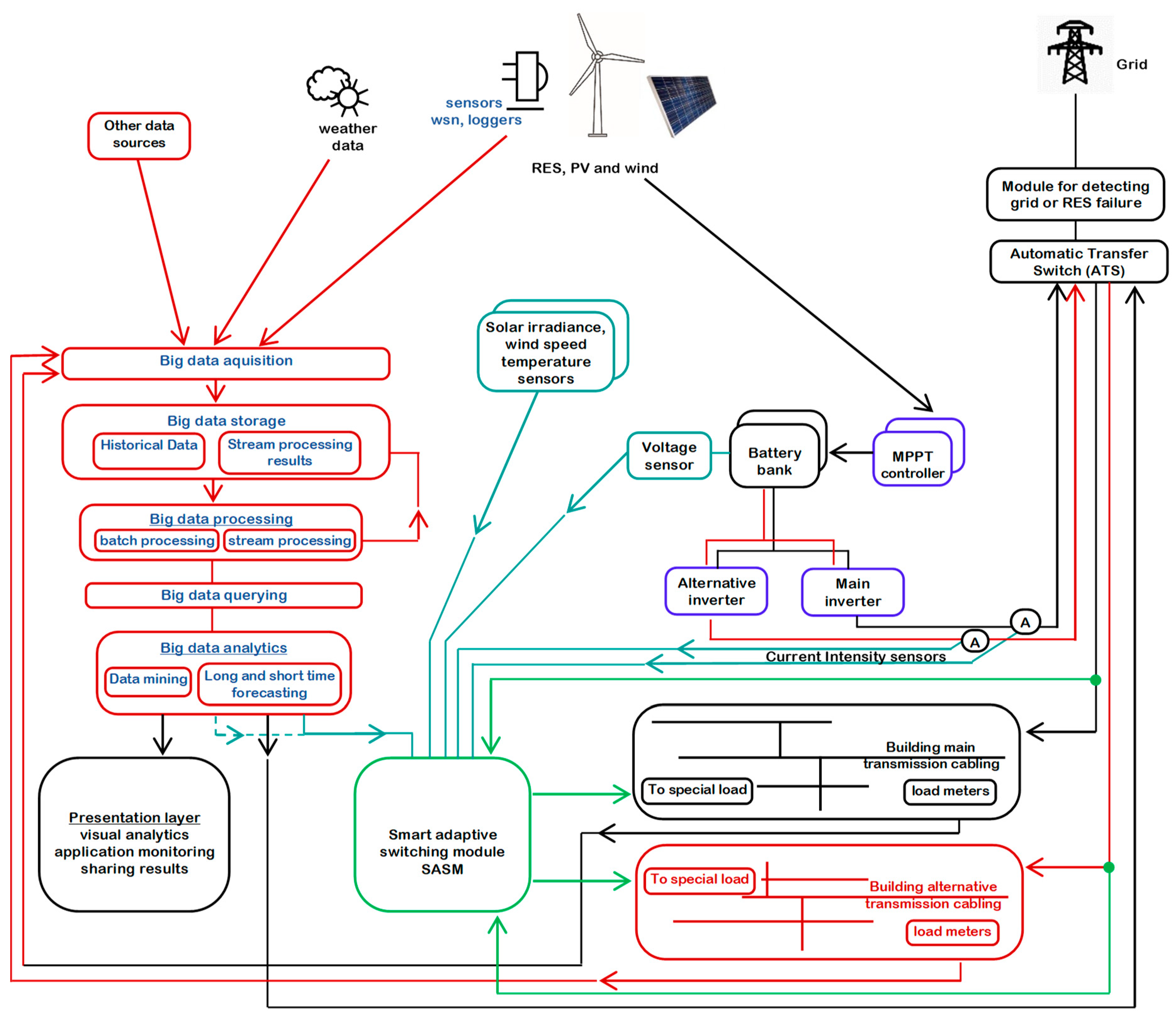
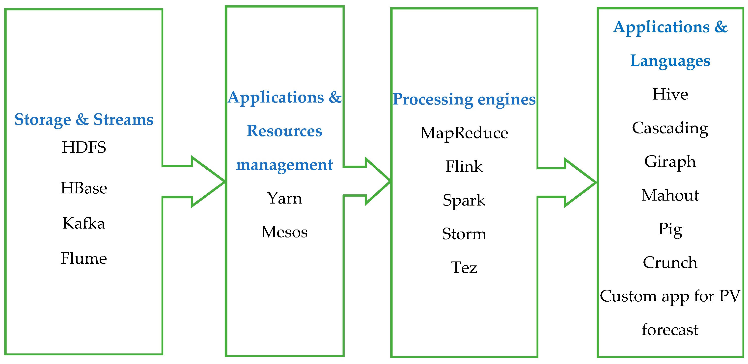
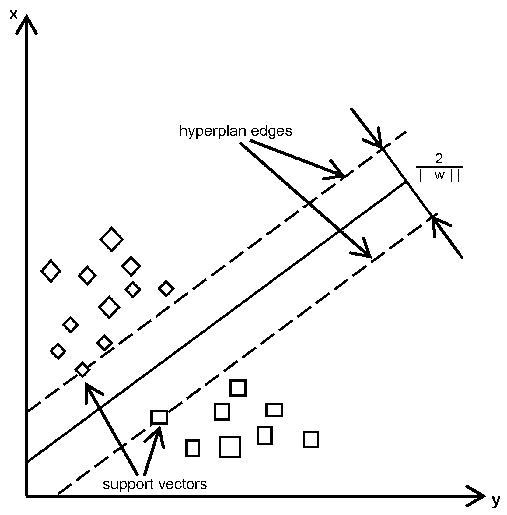
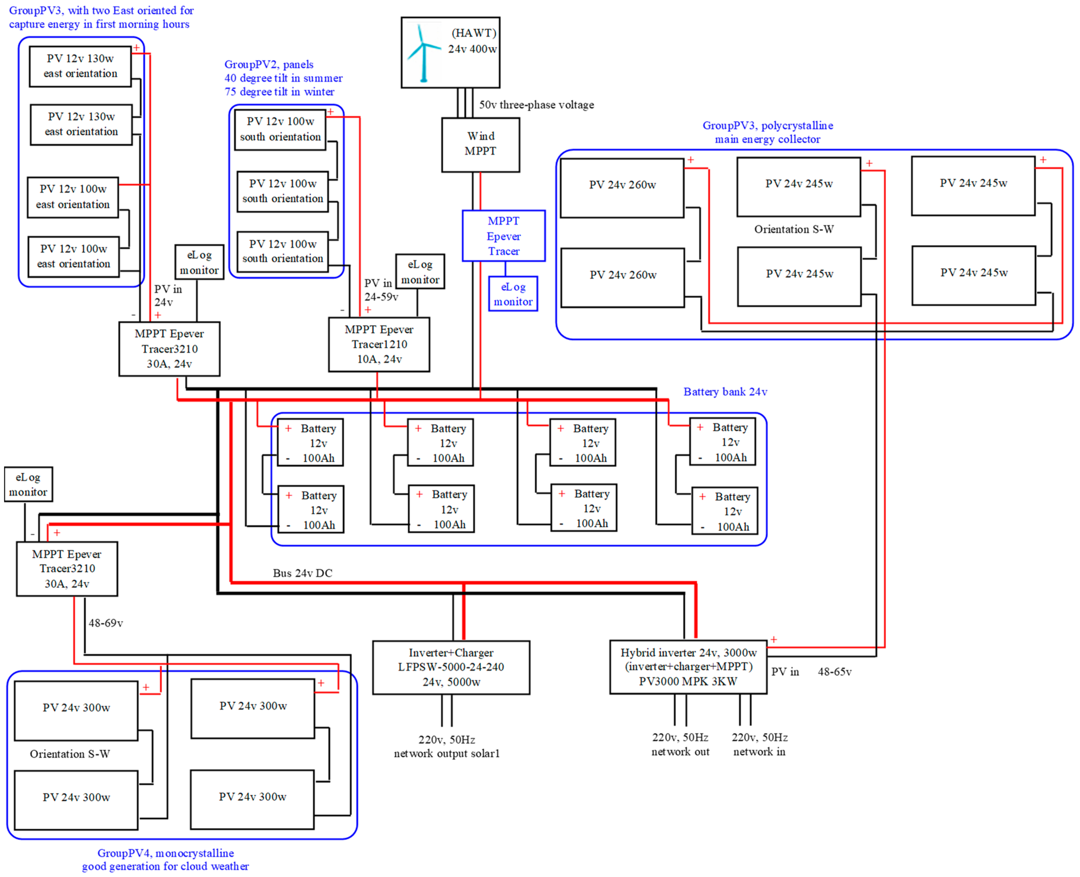
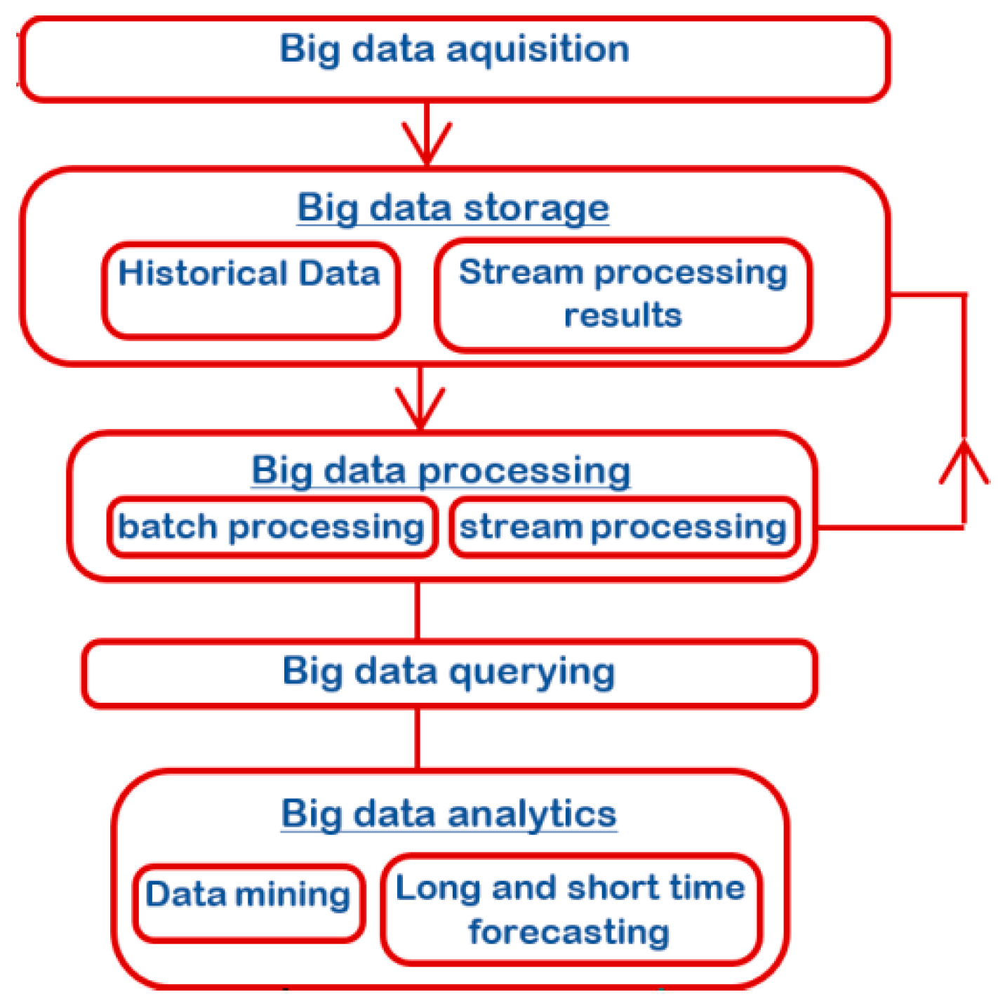
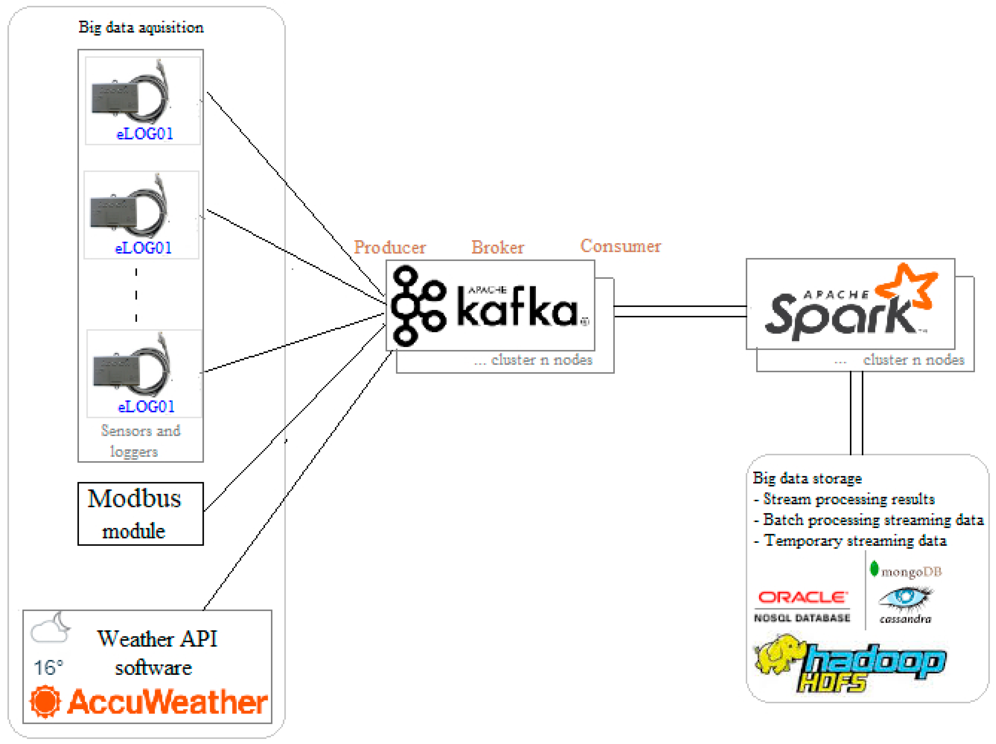
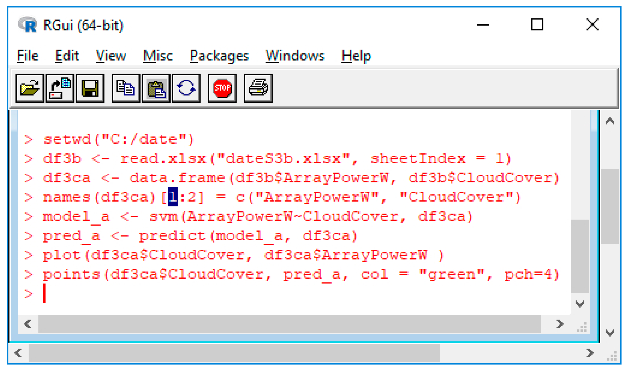
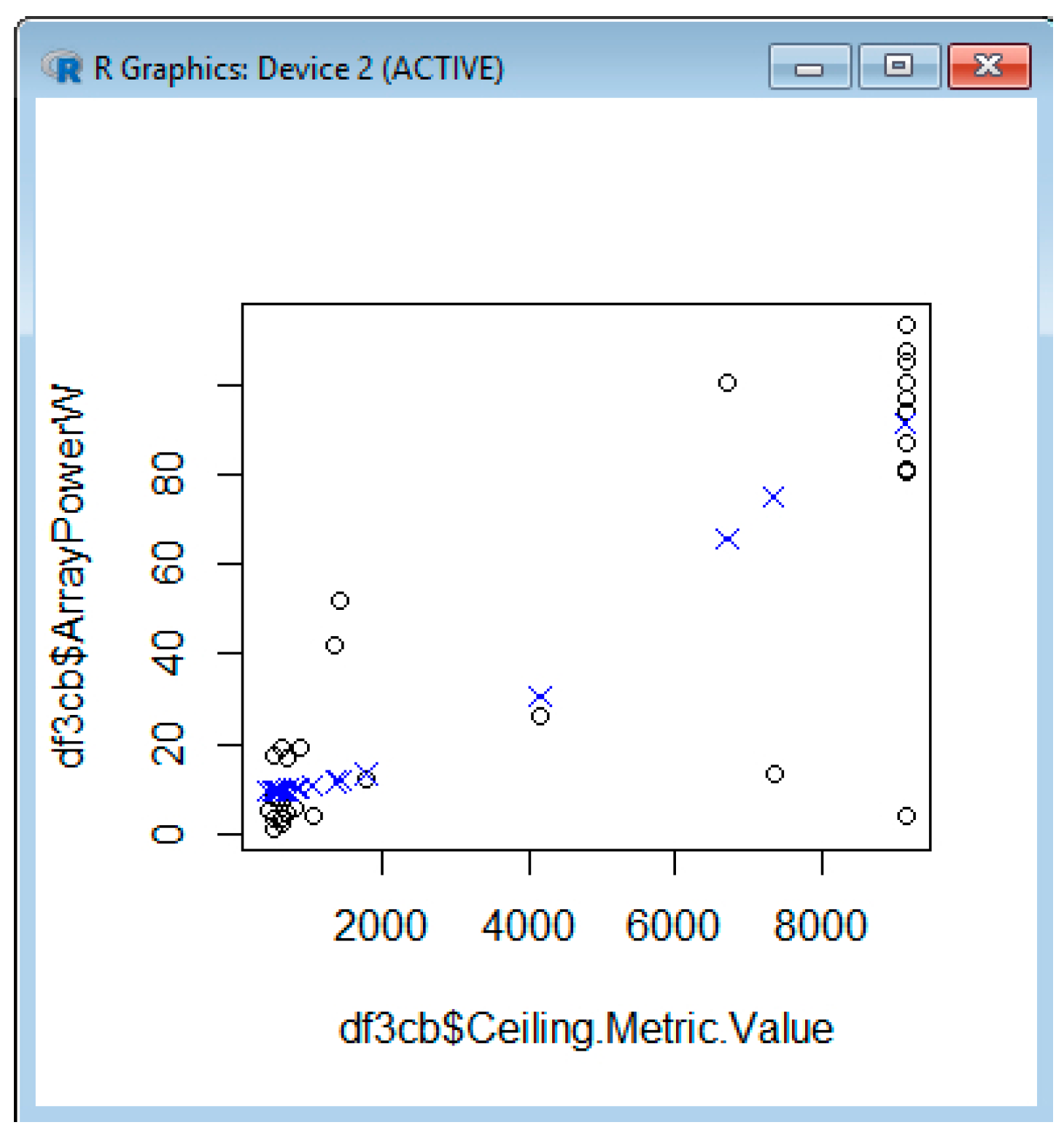
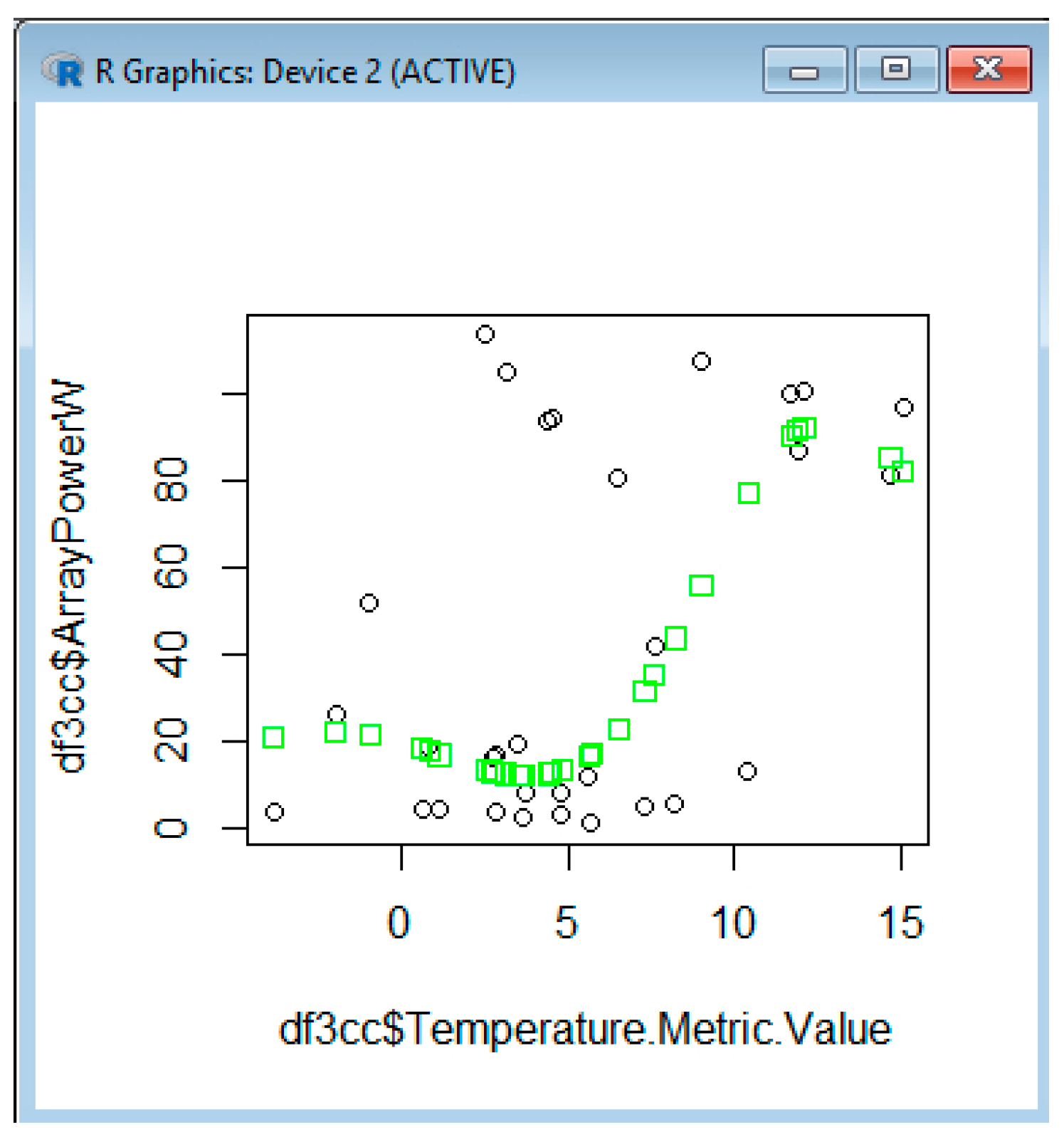
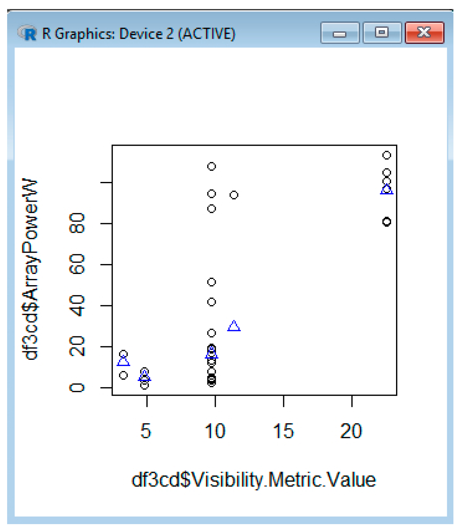
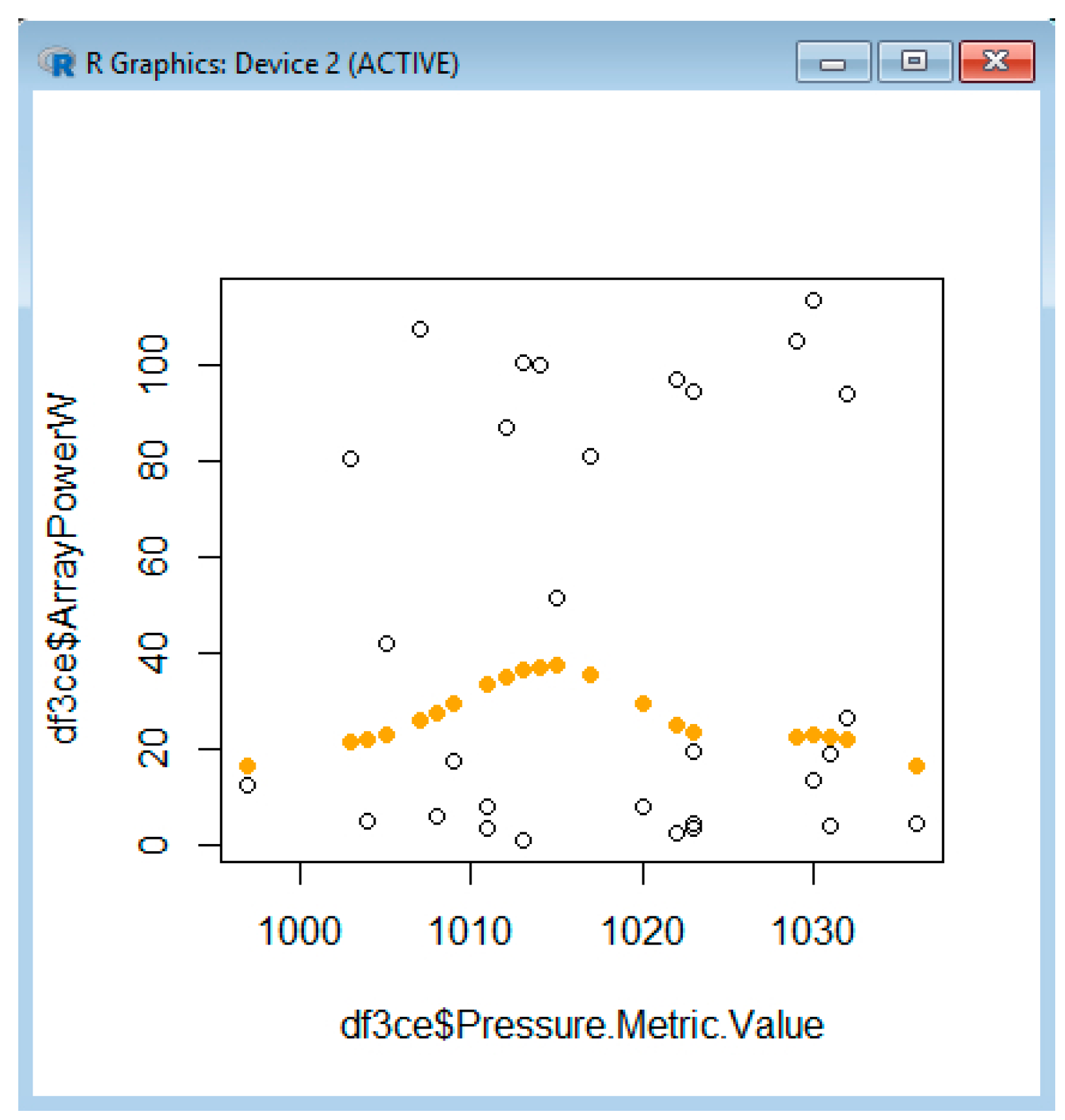
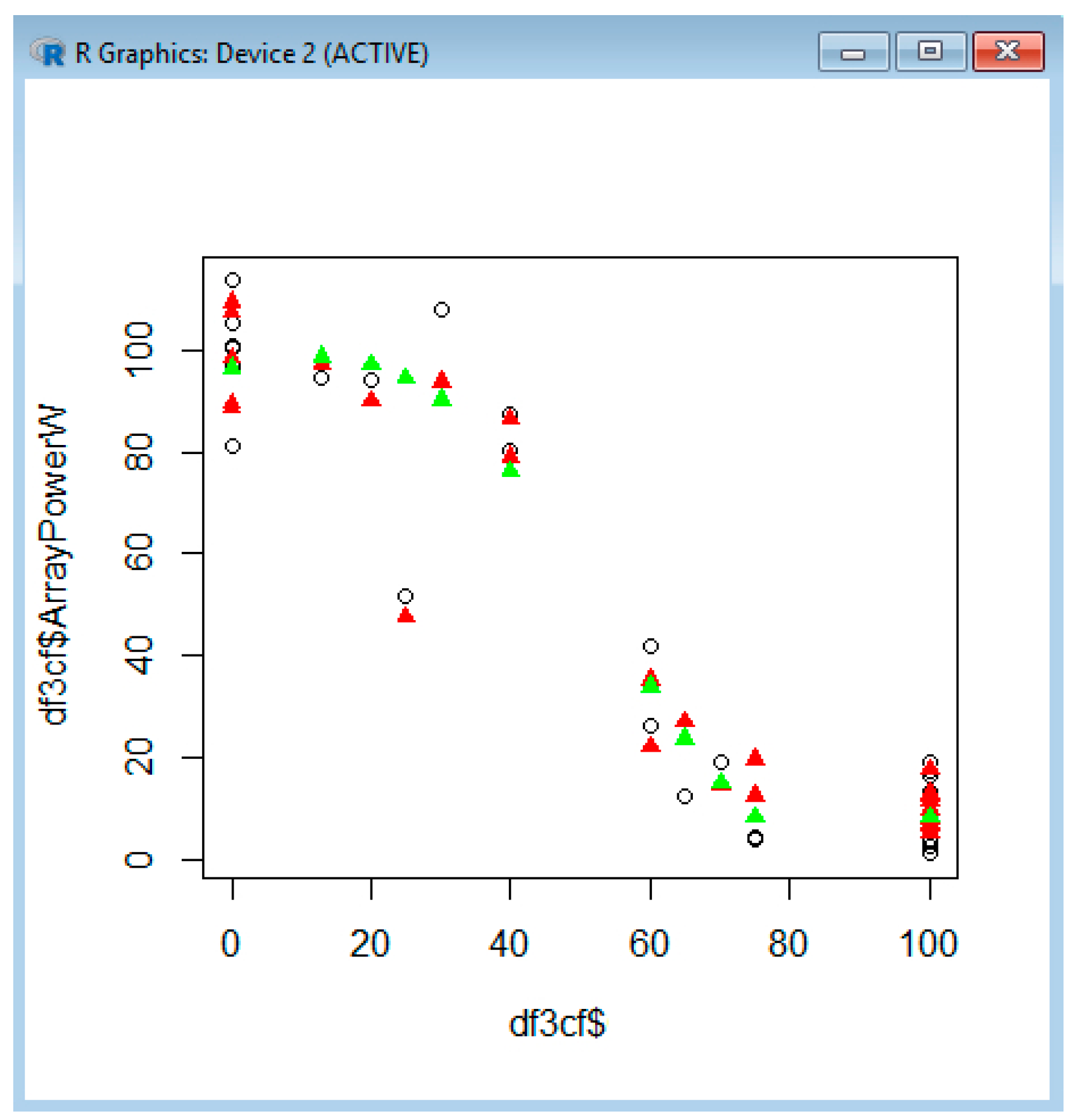
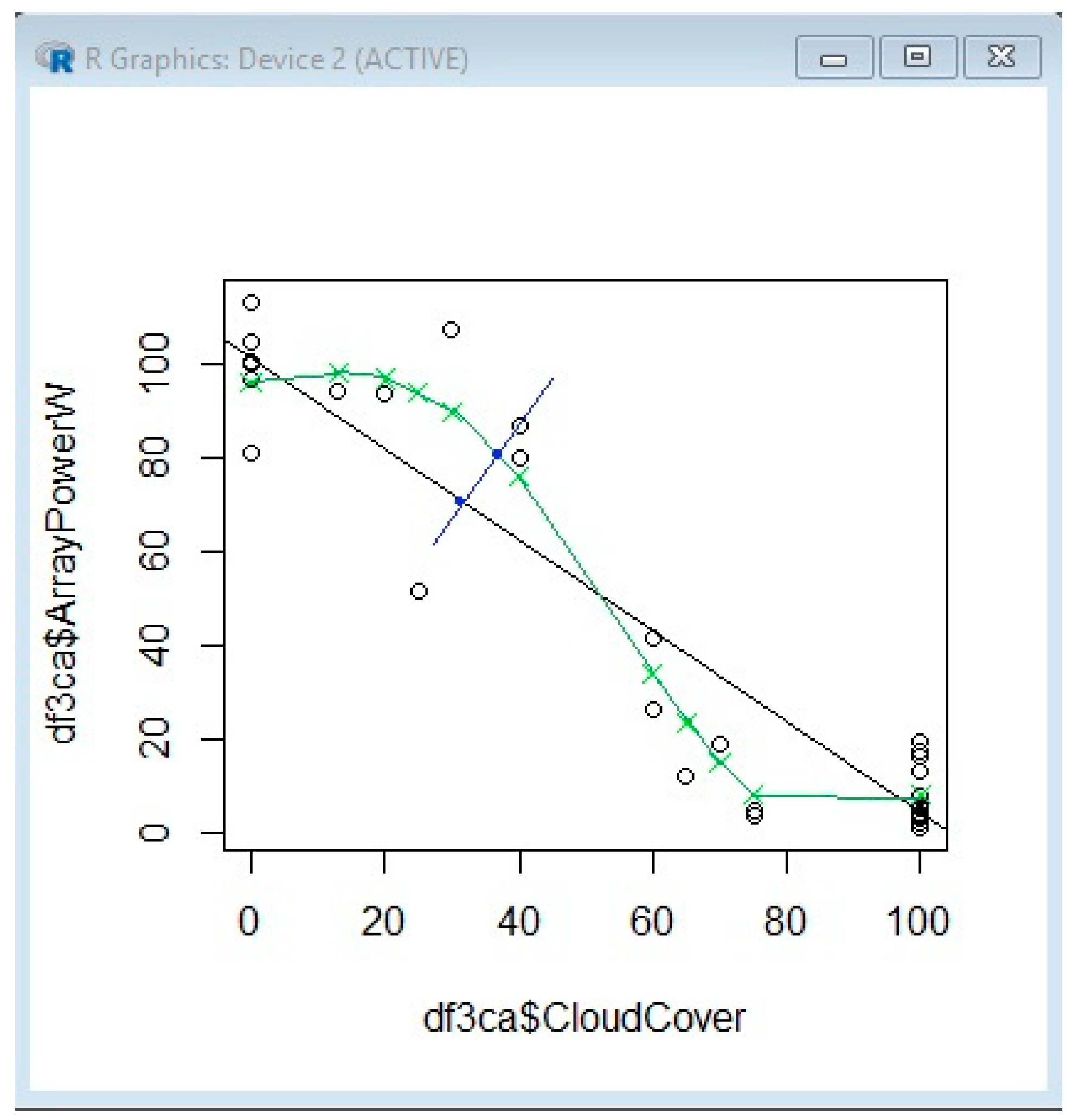
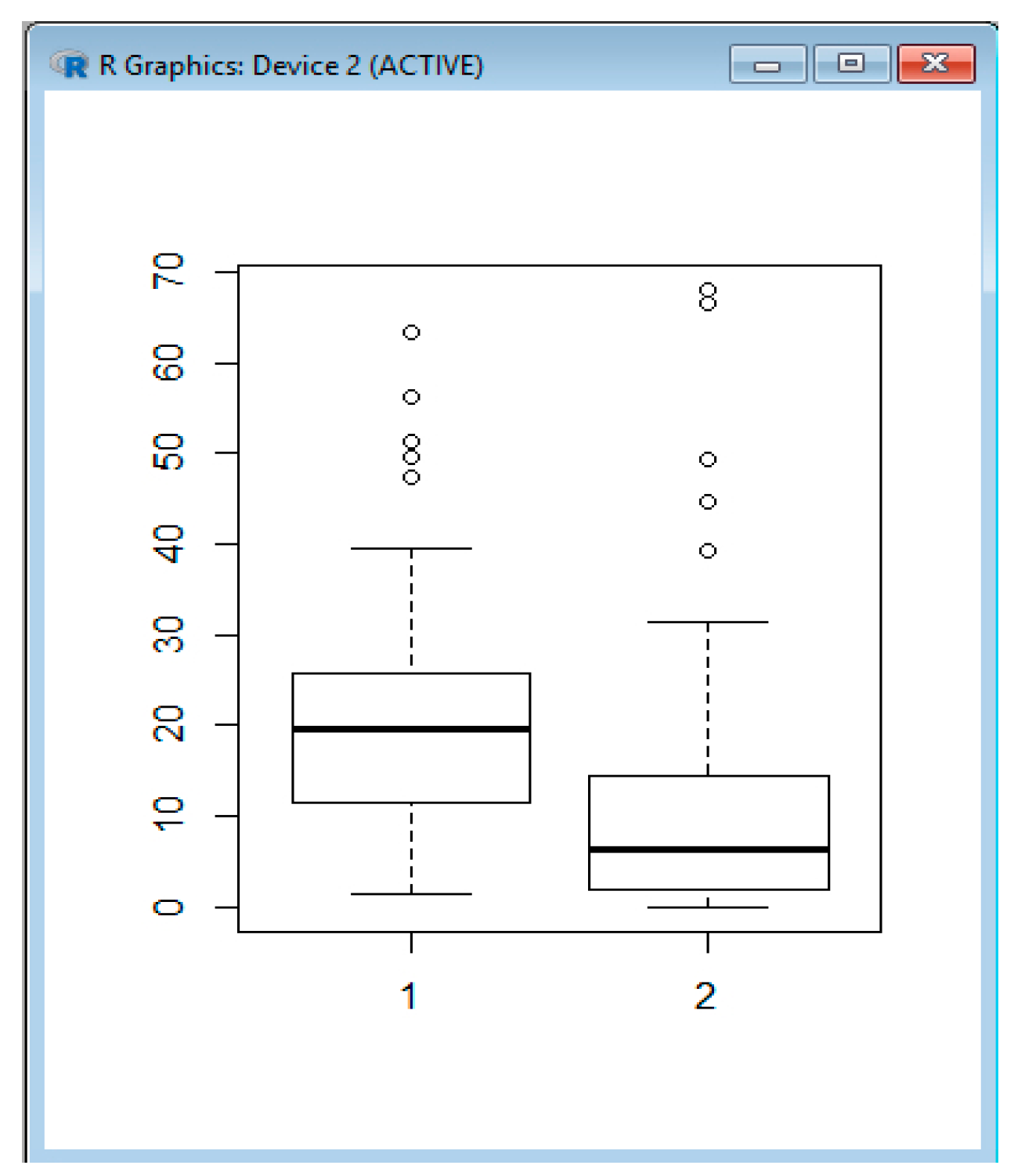
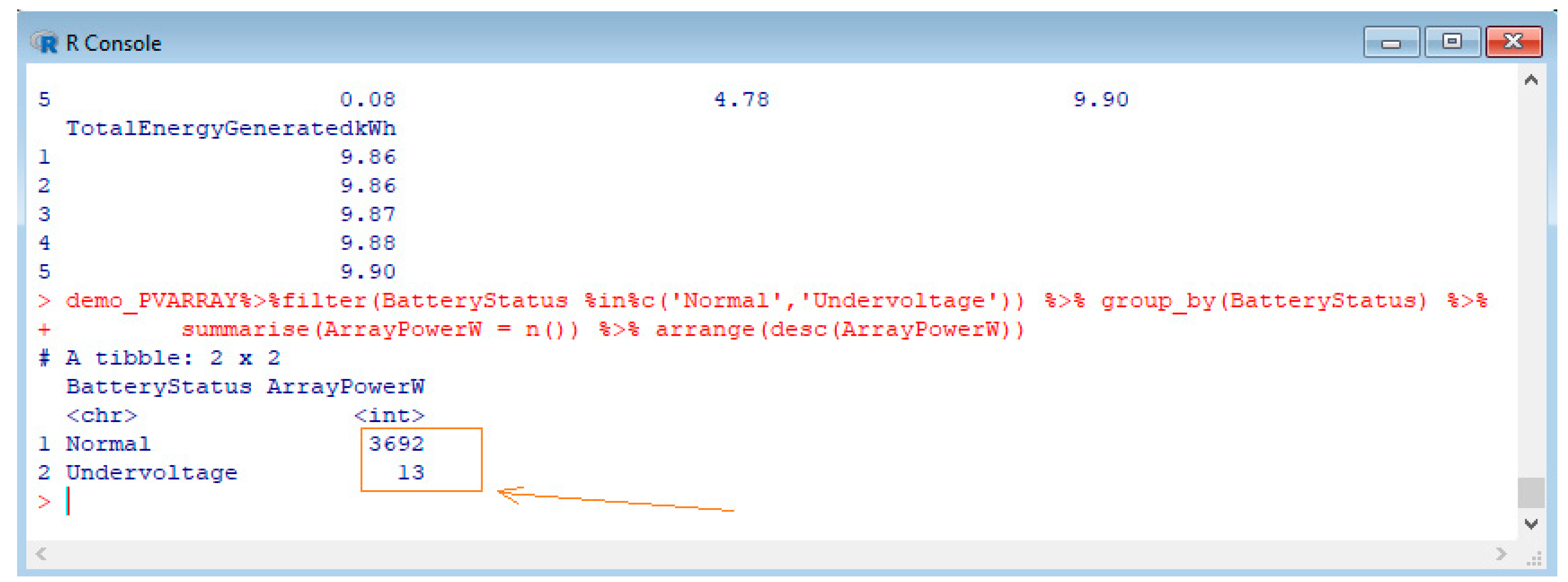
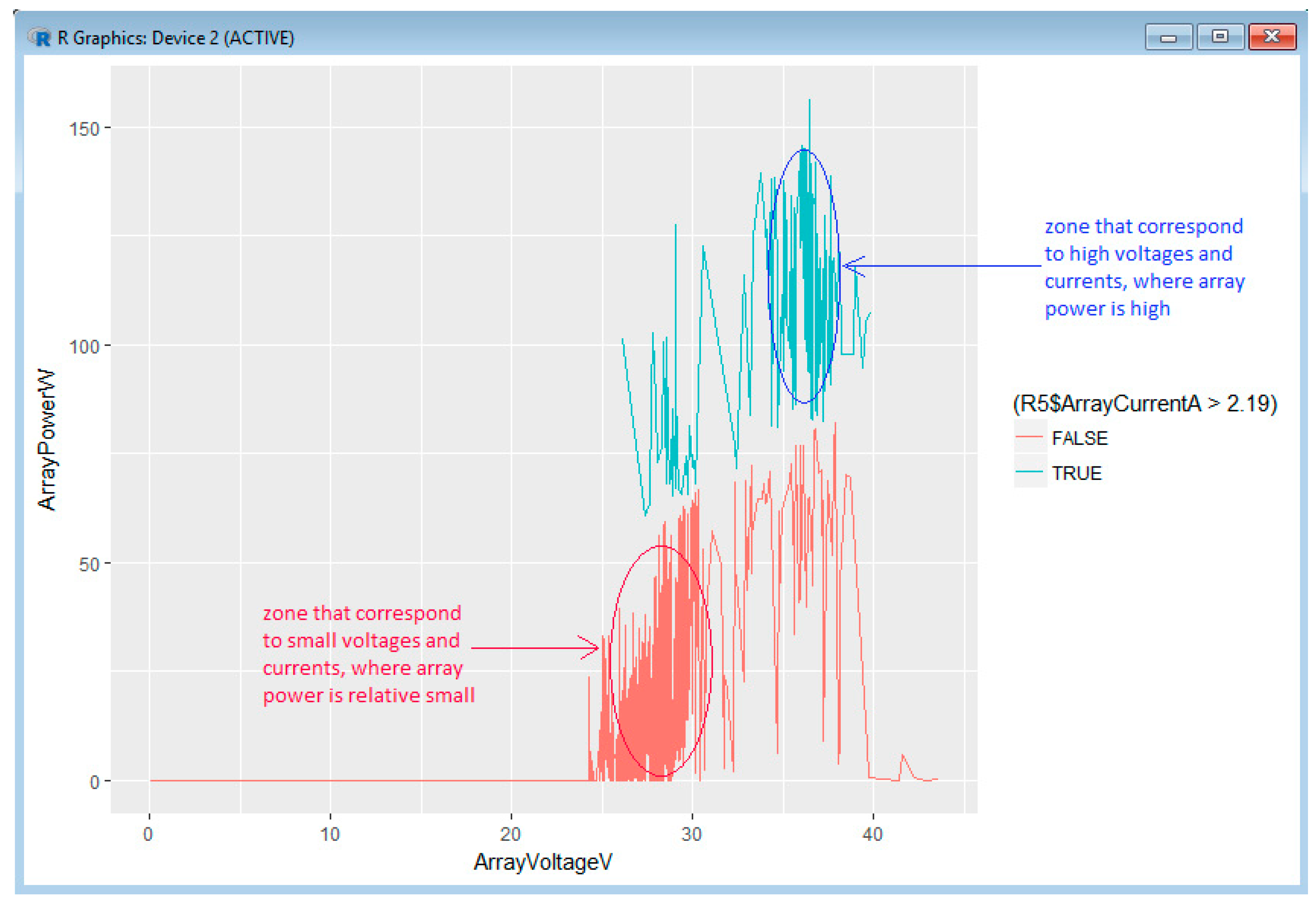
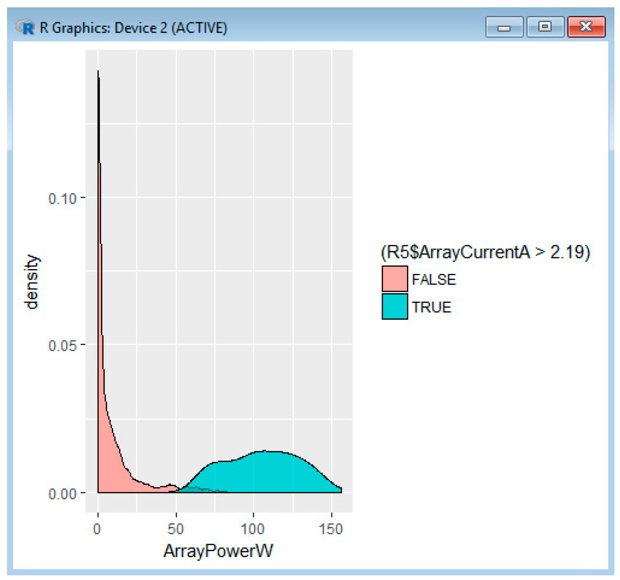
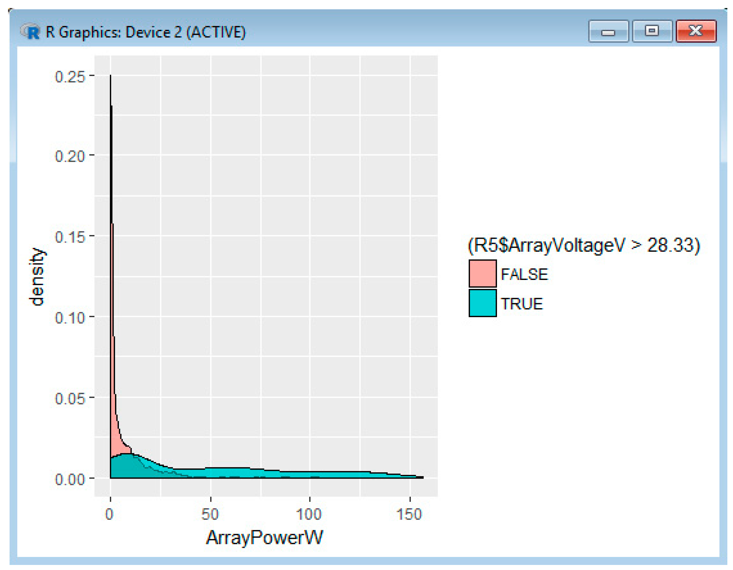
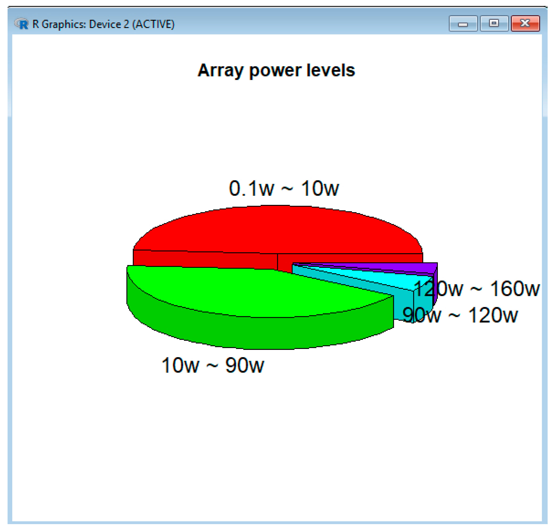
Table 1.
Predicting ArrayPowerW based on ceiling and then ArrayPowerW based on temperature.
| df3cb <- data.frame(df3b$ArrayPowerW, df3b$Ceiling.Metric.Value) | df3cc <- data.frame(df3b$ArrayPowerW, df3b$Temperature.Metric.Value) |
| names(df3cb)[1:2] = c(“ArrayPowerW”, “Ceiling.Metric.Value”) | names(df3cc)[1:2] = c(“ArrayPowerW”, “Temperature.Metric.Value”) |
| model_b <- svm(ArrayPowerW~Ceiling.Metric.Value, df3cb) | model_c <- svm(ArrayPowerW~Temperature.Metric.Value, df3cc) |
| pred_b <- predict(model_b, df3cb) | pred_c <- predict(model_c, df3cc) |
| plot(df3cb$Ceiling.Metric.Value, df3cb$ArrayPowerW) | plot(df3cc$Temperature.Metric.Value, df3cc$ArrayPowerW) |
| points(df3cb$Ceiling.Metric.Value, pred_b, col = “blue”, pch = 4) | points(df3cc$Temperature.Metric.Value, pred_c, col = “green”, pch = 0) |
© 2018 by the authors. Licensee MDPI, Basel, Switzerland. This article is an open access article distributed under the terms and conditions of the Creative Commons Attribution (CC BY) license (http://creativecommons.org/licenses/by/4.0/).
Share and Cite
MDPI and ACS Style
Preda, S.; Oprea, S.-V.; Bâra, A.; Belciu, A. PV Forecasting Using Support Vector Machine Learning in a Big Data Analytics Context. Symmetry 2018, 10, 748. https://0-doi-org.brum.beds.ac.uk/10.3390/sym10120748
AMA Style
Preda S, Oprea S-V, Bâra A, Belciu A. PV Forecasting Using Support Vector Machine Learning in a Big Data Analytics Context. Symmetry. 2018; 10(12):748. https://0-doi-org.brum.beds.ac.uk/10.3390/sym10120748
Chicago/Turabian StylePreda, Stefan, Simona-Vasilica Oprea, Adela Bâra, and Anda Belciu (Velicanu). 2018. "PV Forecasting Using Support Vector Machine Learning in a Big Data Analytics Context" Symmetry 10, no. 12: 748. https://0-doi-org.brum.beds.ac.uk/10.3390/sym10120748
Note that from the first issue of 2016, this journal uses article numbers instead of page numbers. See further details here.