Design of Sampling Plan Using Regression Estimator under Indeterminacy

Abstract

The acceptance sampling plans are one of the most important tools for the inspection of a lot of products. Sometimes, it is difficult to study the variable of interest, and some additional or auxiliary information which is correlated to that variable is available. The existing sampling plans having auxiliary information are applied when the full, precise, determinate and clear data is available for lot sentencing. Neutrosophic statistics, which is the extension of classical statistics, can be applied when information about the quality of interest or auxiliary information is unclear and indeterminate. In this paper, we will introduce a neutrosophic regression estimator. We will design a new sampling plan using the neutrosophic regression estimator. The neutrosophic parameters of the proposed plan will be determined through the neutrosophic optimization solution. The efficiency of the proposed plan is discussed. The results of the proposed plan will be explained using real industrial data. From the comparison, it is concluded that the proposed sampling plan is more effective and adequate for the inspection of a lot than the existing plan, under the conditions of uncertainty.

1. Introduction

In industry, it is necessary to control the presence of defective items in the raw material that may cause rejection of the finished product. For lot sentencing, a random sample is selected from the batch and presence or absence of the defective items is noted on the basis of sample measurements (see [1]). So, the fate of the lot is based on the sample information which, leads to accepting or rejecting the submitted batch of the product. In some industries, such as the cement industry and metal processing, it is hard or costly to measure the quality of interest to make a decision about the batch, so another variable which is correlated with the variable of interest is selected and measured for the lot sentencing (see [2] for example). The study of the variable of interest using the correlated variable improves the precision in the decision (see [3]). Aslam et al. [4] introduced a regression estimator in the area of the sampling plan.

There are two major types of acceptance sampling plan, known as an attribute sampling plan and a variable sampling plan. The attribute sampling plan is easy, cheap and time-saving but consists of less information than the variable sampling plans. Whatever the type of sampling plans, two risks are always linked with acceptance sampling plans. The probability of rejecting a good lot/accepting a bad lot is called the producer’s risk/consumer’s risk, respectively. Several authors worked on the design variable sampling plans for various situations using classical statistics, the reader may refer to [5,6,7].

In practice, when there is uncertainty in percentage of the product which is defective, the traditional sampling plans can be applied for a lot sentencing purpose. In this situation, a sampling plan using fuzzy logic can be applied for the inspection of a lot of product. Several authors contributed in this area to develop fuzzy sampling plans. In single attribute sampling, the plan parameters do not exactly meet the given producer’s risk and consumer’s risk. Kanagawa and Ohta [8] designed a single attribute fuzzy sampling plan and presented a fuzzy mathematical program for this case. Jamkhaneh et al. [9] worked on a fuzzy rectifying single sampling plan and introduced average outgoing quality (AOQ) and average total inspection (ATI) under the fuzzy sets theory. Jamkhaneh et al. [10] discussed the effect of sampling error under a fuzzy environment and showed that sampling with inspection error has lower operating characteristics (OC) curve band than the sampling plan without inspection error. Jamkhaneh et al. [11] proposed the sampling plan when the proportion parameter is fuzzy, and discussed various bands in the OC curve. Tong and Wang [12] presented the plan for the inspection of geospatial data having ambiguous characteristics when fraction non-conforming and sample rate are fuzzy. Turanoğlu [13] proposed a sampling plan for when the parameters in practice are not crisp values and are expressed by linguistic variables. Uma and Ramya [14] discussed the impact of the fuzzy approach on the sampling plan. They presented a detailed review of fuzzy acceptance sampling plans. Kahraman et al. [15] presented multi-objective mathematical models for the single and the double acceptance sampling plans to solve the complex quality issues. Afshari and Sadeghpour Gildeh [16] proposed a fuzzy sampling plan for the in-decision state and compared their plan with the fuzzy single sampling, the fuzzy double sampling plan, and fuzzy sequential sampling plan.

According to reference [17], “observations include human judgments, and evaluations and decisions, a continuous random variable of a production process should include the variability caused by human subjectivity or measurement devices, or environmental conditions. These variability causes create vagueness in the measurement system. In this situation, the data is recorded in range rather than an exact value of variable under study. Therefore, the analysis based on classical statistics does not represent the real system adequately”. Smarandache [18] mentioned that neutrosophic logic is the generalization of fuzzy logic. The sampling plan having auxiliary information cannot be applied for lot sentencing when the sample information is uncertain, incomplete and indeterminate. Sometimes, we are uncertain about the sample size required for the inspection of a lot of the product and related acceptance number. So, we do not express this information in a crisp value using the classical information (see [19]). Neutrosophic statistics, which is the extension of classical statistics, can be applied when information about the quality of interest or auxiliary information is unclear, indeterminate, uncertain and incomplete. Recently, Aslam [20] introduced neutrosophic statistics in the area of statistical quality control. Aslam and Arif [21] designed the sudden death test under neutrosophic statistics. Aslam [22] designed the sampling plan for the exponential distribution using neutrosophic statistics. Aslam and Raza [23] proposed the plan for multiple manufacturing lines using neutrosophic statistics. By following [24], the authors’ contributions towards the sampling plan can be seen in the

Table 1. Contribution towards the sampling plans.

Authors	Year	Contributions
Aslam et al. [4]	2017	Introduced regression estimator in the sampling plan
Smarandache [18]	2010	Introduced neutrosophic logic
Smarandache [25]	2014	Introduced neutrosophic statistics
Aslam [20]	2018	Introduced neutrosophic industrial statistics (NIS)

.

The existing sampling plans using classical statistics are used when all the observations in the sample or the population are determined. In practice, under the uncertainty environment, it may be that some observations in the sample or in the population are uncertain. In the latter case, the sampling plan using the regression estimator under classical statistics cannot be appalled.

We did not find plans using the neutrosophic regression estimator in the literature. We hope that neutrosophic acceptance sampling plans using the neutrosophic regression estimator will be more helpful for industrial engineers for lot sentencing in indeterminate environments. In this paper, we will introduce the neutrosophic regression estimator. We will design a new sampling plan using the neutrosophic regression estimator. The neutrosophic parameters of the proposed plan will be determined through a neutrosophic optimization solution. The results of the proposed plan will be explained by real data from industry.

2. Design of the Proposed Plan

Let $y_{NN}\mathsf{ϵ}\left\{y_L,y_U\right\}$ be a neutrosophic random variable, where $y_L$ and $y_U$ denote the lower observation and upper observation, respectively, and quality of interest $y_{NN}$ follows the neutrosophic normal distribution with neutrosophic mean ${\mu }_{Ny }\mathsf{ϵ}\left\{{\mu }_{Ly},{\mu }_{Uy}\right\}$ and unknown neutrosophic standard deviation ${\sigma }_{Ny }\mathsf{ϵ}\left\{{\sigma }_{Ly},{\sigma }_{Uy}\right\}$. Suppose that $x_{NN}$ be neutrosophic auxiliary variable follows the neutrosophic normal distribution with neutrosophic mean ${\mu }_{Nx}\mathsf{ϵ}\left\{{\mu }_{Lx},{\mu }_{Ux}\right\}$ and unknown neutrosophic standard deviation ${\sigma }_{Nx}\mathsf{ϵ}\left\{{\sigma }_{Lx},{\sigma }_{Ux}\right\}$. Suppose that $\left(y_{N1},x_{N1}\right),\left(y_{N2},x_{N2}\right),\dots , \left(y_{Nn},x_{Nn}\right)$ be a bivariate neutrosophic random variable. From [25], we defined neutrosophic correlation $r_N$ as follows

$$r_N=\frac{n_N\sum xy-\sum x\sum y}{\sqrt{\{n_N\sum x^2-{\left(\sum x\right)}^2\}\{n_N\sum y^2-{\left(\sum y\right)}^2\}}};n_N\mathsf{ϵ}\left\{n_L,n_U\right\}$$

(1)

The neutrosophic regression estimator $M_{Nr}$ is defined as

$$M_{Nr}={\overline{Y}}_N+b_N\left({\mu }_{Nx}-{\overline{X}}_N\right);{\overline{X}}_N\mathsf{ϵ}\left\{{\overline{X}}_L,{\overline{X}}_U\right\}, {\overline{Y}}_N\mathsf{ϵ}\left\{{\overline{Y}}_L,{\overline{Y}}_U\right\}, b_N\mathsf{ϵ}\left\{b_L,b_U\right\}$$

(2)

where ${\overline{Y}}_N$ and ${\overline{X}}_N$ are neutrosophic mean for $y_{NN}$ and $x_{NN}$, respectively. The neutrosophic regression coefficient $b_N$ is defined by

$$b_N=r_{Nxy}\frac{{\mathrm{S}}_{Ny}}{{\mathrm{S}}_{Nx}},{\mathrm{S}}_{Ny}=\left\{s_{Ly},s_{Uy}\right\},r_{Nxy}=\left\{r_{NxyL},r_{NxyU}\right\},{\mathrm{S}}_{Nx}=\left\{s_{Lx},s_{Ux}\right\}$$

(3)

where ${\overline{X}}_L={{\displaystyle \sum }}_{i=1}^n{x}_i^L/n_L,$ ${\overline{X}}_U={{\displaystyle \sum }}_{i=1}^n{x}_i^U/n_U$, $s_{Lx}=\sqrt{{{\displaystyle \sum }}_{i=1}^n{\left(x_i^L-{\overline{X}}_L\right)}^2/n_L}$, $s_{Ux}=\sqrt{{{\displaystyle \sum }}_{i=1}^n{\left(x_i^U-{\overline{X}}_U\right)}^2/n_U}$, ${\overline{Y}}_L={{\displaystyle \sum }}_{i=1}^n{Y}_i^L/n_L,{\overline{Y}}_U={{\displaystyle \sum }}_{i=1}^n{Y}_i^U/n_U$, $s_{Ly}=\sqrt{{{\displaystyle \sum }}_{i=1}^n{\left(Y_i^L-{\overline{Y}}_L\right)}^2/n_L}$ and $s_{Uy}=\sqrt{{{\displaystyle \sum }}_{i=1}^n{\left(Y_i^U-{\overline{Y}}_U\right)}^2/n_U}$.

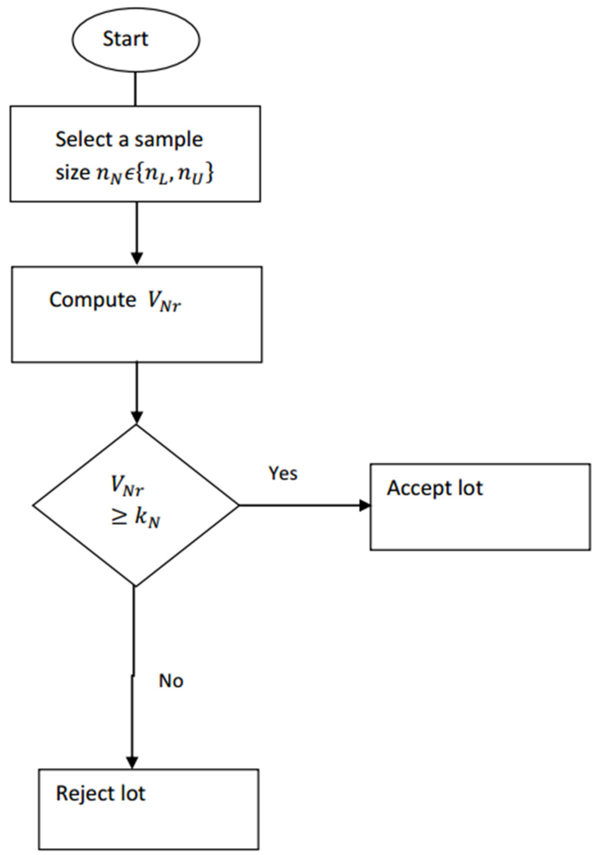
We proposed the following plan based on the neutrosophic regression estimator as

Step #1. Measure the bivariate quality characteristics $\left(y_{N1},x_{N1}\right),\left(y_{N2},x_{N2}\right),\dots , \left(y_{Nn},x_{Nn}\right)$ based on the sample size $n_N.$ Compute following the neutrosophic statistic $M_{Nr}$.

Step #2. Calculate $V_{Nr}=\frac{USL -M_{Nr}}{{\widehat{\sigma }}_{M_{Nr}}}$; ${\widehat{\sigma }}_{M_{Nr}}\mathsf{ϵ}\left\{{\widehat{\sigma }}_{M_y},{\widehat{\sigma }}_{M_x}\right\}$

where

$${\widehat{\sigma }}_{M_{Nr}}=\sqrt{S_{Ny}^2\left(1-r_{Nxy}^2\right)\left(1+1/\left(n_N-3\right)\right)/n_N}$$

Step #3. Accept the lot if $V_{Nr}\ge k_N$, where $k_{N }\mathsf{ϵ}\left\{k_{aL},k_{aU}\right\}$ is the neutrosophic acceptance number.

The proposed neutrosophic auxiliary variable plan is based on two neutrosophic parameters, namely $n_N$ = $\left\{n_L,n_U\right\}$ and $k_{N }\mathsf{ϵ}\left\{k_{aL},k_{aU}\right\}$. The operational process of the proposed sampling plan can be seen in the Figure 1. The proposed sampling plan reduces to Aslam et al. [4] when there are no uncertain observations in the data. Here we define the null hypothesis that the product is good vs. the alternative hypothesis that the product is not good. These hypotheses are tested using the sample information. We accept the null hypothesis if $V_{Nr}\ge k_N$, otherwise, we accept the alternative hypothesis and declare that the product is bad. According to the plan, a lot will be accepted if $V_{Nr}\ge k_N$. Therefore, the neutrosophic operating characteristic function (NOCF) of the proposed plan is derived as follows

$$L\left(p\right)=P\left(V_{Nr}\ge k_N\right)=P\left\{M_{Nr}+k_N{\widehat{\sigma }}_{M_{Nr}}\right\},k_N\mathsf{ϵ}\left\{k_{aL},k_{aU}\right\}, {\widehat{\sigma }}_{M_{Nr}}\mathsf{ϵ}\left\{{\widehat{\sigma }}_{M_y},{\widehat{\sigma }}_{M_x}\right\}$$

(4)

Following [3], $M_{Nr}$ follows the approximate neutrosophic normal distribution, that is, $M_{Nr}~N_N\left({\mu }_{Ny}, {\sigma }_{Ny}^2\left(1-r_{Nxy}\right)\left(1+1/\left(n_N-3\right)\right)/n_N\right)$; $r_{Nxy}=\left\{r_{NxyL},r_{NxyU}\right\}$. According to [26] $M_{Nr}\pm k_N{\widehat{\sigma }}_{M_{Nr}}$ has following a neutrosophic normal distribution $M_{Nr}\pm k_N{\widehat{\sigma }}_{M_{Nr}}~N_N\left(E\left[M_{Nr}\right]\pm k_{N}E\left[{\widehat{\sigma }}_{M_{Nr}}\right],V\left[M_{Nr}\right]\pm k_N^{2}V\left[{\widehat{\sigma }}_{M_{Nr}}\right]\right)$, $k_N\mathsf{ϵ}\left\{k_{aL},k_{aU}\right\}$, ${\widehat{\sigma }}_{M_{Nr}}\mathsf{ϵ}\left\{{\widehat{\sigma }}_{M_y},{\widehat{\sigma }}_{M_x}\right\}$.

Following [4], the neutrosophic mean and variance of ${\widehat{\sigma }}_{M_{Nr}}$ are given by

$$E\left({\widehat{\sigma }}_{M_{Nr}}\right)=k_2{c}_4{\sigma }_{\mathrm{Ny}}/\sqrt{n_N}\mathrm{and}V\left({\widehat{\sigma }}_{M_{Nr}}\right)=\frac{k_2^2}{n}{\sigma }_{Ny}^2\left(1-c_4^2\right)$$

(5)

where $c_{4N}={\left[2/\left(n_N-1\right)\right]}^{1/2}\mathsf{\Gamma }\left(n_N/2\right)/\mathsf{\Gamma }\left[n_N-1/2\right]$; $n_N=\{n_L,n_U\}$ and $k_2=\sqrt{(1-{\rho }_{Nxy}^2)\left(1+1/\left(n_N-3\right)\right)}$ is a constant.

So, the neutrosophic normal distribution for $M_{Nr}\pm k_N{\widehat{\sigma }}_{M_{Nr}}$; ${\widehat{\sigma }}_{M_{Nr}}\mathsf{ϵ}\left\{{\widehat{\sigma }}_{M_y},{\widehat{\sigma }}_{M_x}\right\}$, $k_N\mathsf{ϵ}\left\{k_{aL},k_{aU}\right\}$ is given by

$$M_{Nr}+k_N{\widehat{\sigma }}_{M_{Nr}}~N\left({\mu }_{Ny}+q_N{\sigma }_{Ny},{\sigma }_{Ny}^2{U}_N\right)$$

where $U_N=\left[Q_N\left(1-{\rho }_{Nxy}^2\right)+k_N^2\frac{k_2^2}{n_N}\left(1-c_4^2\right)\right]$, $Q_N=\left(1+1/\left(n_N-3\right)\right)/n_N$ and $q_N=k_N{k}_2{c}_{4N}/\sqrt{n_N}$.

The NOCF, say $L\left(p\right)$ using the neutrosophic statistics is given by

$$L\left(p\right)=\mathsf{\Phi }\left\{\frac{USL-{\mu }_{Ny}-q_N{\sigma }_{Ny}}{{\sigma }_{Ny}\sqrt{U_N}}\right\}=\mathsf{\Phi }\left\{\left(\frac{USL-{\mu }_{Ny}}{{\sigma }_{Ny}}-q_N\right)/\sqrt{U_N}\right\}$$

(6)

Suppose $Z_{N_{pU}}=\frac{USL-{\mu }_{Ny}}{{\sigma }_{Ny}}$ is the neutrosophic standard normal variable, so, the final NOCF is given by

$$L\left(p\right)=\mathsf{\Phi }\left\{\left(Z_{N_{pU}}-q_N\right)/\sqrt{U_N}\right\}$$

(7)

To meet the customer and producer satisfaction, the plan parameters of the proposed plan must satisfy the producer’s risk, say $\alpha$ at acceptable quality level (AQL) at $p_1$ and customer’s risk, say $\beta$ ay limiting quality level (LQL) at $p_2$. So, the plan parameters $k_{N }\mathsf{ϵ}\left\{k_{aL},k_{aU}\right\}$ and $n_N\mathsf{ϵ}\left\{n_L,n_U\right\}$ of the proposed plan will be determined using the following neutrosophic optimization solution given in Equations (8)–(10).

$$\mathrm{minimize}{n}_N\mathsf{ϵ}\left\{n_L,n_U\right\}$$

(8)

subject to

$$L_N\left(p_1\right)=\mathsf{\Phi }\left\{\left(Z_{N_{pU1}}-q_N\right)/\sqrt{U_N}\right\}\ge 1-\alpha ;k_{N }\mathsf{ϵ}\left\{k_{aL},k_{aU}\right\};n_N\mathsf{ϵ}\left\{n_L,n_U\right\}$$

(9)

and

$$L_N\left(p_2\right)=\mathsf{\Phi }\left\{\left(Z_{N_{pU2}}-q_N\right)/\sqrt{U_N}\right\}\le \beta ;k_N\mathsf{ϵ}\left\{k_{aL},k_{aU}\right\};n_N\mathsf{ϵ}\left\{n_L,n_U\right\}$$

(10)

Table 2. The plan parameters of the plan when $\alpha =0.05$, $\beta$ = 0.10 and $r_{Nxy}=\left\{0.7817,0.8319\right\}$.

${\mathit{p}}_1$	${\mathit{p}}_2$	${\mathit{n}}_{\mathit{N}}$	${\mathit{k}}_{\mathit{N}}$	${\mathit{L}}_{\mathit{N}}\left({\mathit{p}}_1\right)$	${\mathit{L}}_{\mathit{N}}\left({\mathit{p}}_2\right)$
0.001	0.004	[321,323]	[93.9,105.2]	[0.9505,0.9512]	[0.0991,0.0999]
	0.006	[184,186]	[69.7,77.9]	[0.9533,0.9539]	[0.0967,0.0968]
	0.008	[128,130]	[59.9,64.5]	[0.9503,0.9515]	[0.0929,0.0983]
	0.010	[102,106]	50.1,57.5]	[0.9524,0.9544]	[0.0878,0.0973]
	0.015	[71,73]	[40.6,46.2]	[0.9596,0.9645]	[0.0968,0.0990]
	0.020	[55,77]	[35.1,40.1]	[0.9576,0.9633]	[0.0919,0.0954]
0.0025	0.030	[62,65]	[34.9,40.0]	[0.9561,0.9655]	[0.0959,0.0966]
	0.050	[38,40]	[26.2,30.3]	[0.9553,0.9587]	[0.0846,0.0955]
0.005	0.050	[55,59]	[30.6,35.8]	[0.9515,0.9539]	[0.0788,0.0955]
	0.100	[30,33]	[21.0,24.3]	[0.9639,0.9819]	[0.0900,0.0963]
	0.140	[23,25]	[17.4,20.1]	[0.9752,0.9865]	[0.0983, 0.0994]
0.01	0.030	[233,235]	[63.5,71.7]	[0.9501,0.9518]	[0.0931,0.0978]
0.03	0.090	[134,136]	[40.6,45.9]	[0.9516,0.9576]	[0.0974,0.0986]
0.05	0.100	[285,290]	[56.3,63.9]	[0.9538,0.9552]	[0.0902,0.0998]
	0.150	[115,118]	[33.7,38.3]	[0.9739,0.9788]	[0.0959,0.0989]

shows the plan parameters $n_N\mathsf{ϵ}\left\{n_L,n_U\right\}$, $k_N\mathsf{ϵ}\left\{k_{aL},k_{aU}\right\}$ of the proposed plan at different levels of AQL and LQL. The plan parameters presented in Table 2 are obtained through the above stated neutrosophic optimization solution by using a search grid method. The probabilities of acceptance at producer’s risk and consumer’s risk are also shown in Table 2 and

Table 3. The plan parameters of the plan when $\alpha =0.05$, $\beta$ = 0.10 and $r_{Nxy}=\left\{0.88,0.90\right\}$.

${\mathit{p}}_1$	${\mathit{p}}_2$	${\mathit{n}}_{\mathit{N}}$	${\mathit{k}}_{\mathit{N}}$	${\mathit{L}}_{\mathit{N}}\left({\mathit{p}}_1\right)$	${\mathit{L}}_{\mathit{N}}\left({\mathit{p}}_2\right)$
0.001	0.004	[264,299]	[104.6,121.0]	[0.9532,0.9682]	[0.0903,0.0846]
	0.006	[161,172]	[79.3,89.6]	[0.9672,0.9690]	[0.0904,0.0769]
	0.008	[115,129]	[66.3,76.3]	[0.9568,0.9707]	[0.0705,0.0655]
	0.01	[99,103]	[60.2,66.3]	[0.9725,0.9831]	[0.0728,0.0858]
	0.02	[61,63]	[43.3,48.8]	[0.9947,0.9918]	[0.0977,0.0700]
0.0025	0.03	[53,57]	[38.7,43.8]	[0.9685,0.9738]	[0.0746,0.0663]
	0.05	[39,41]	[30.2,35.6]	[0.9945,0.9801]	[0.0995,0.0438]
0.005	0.05	[47,58]	[33.7,40.9]	[0.9630,0.9766]	[0.0631,0.0425]
	0.1	[24,33]	[21.6,27.3]	[0.9806,0.9955]	[0.0731,0.0514]
0.005	0.14	[23,30]	[18.7,27.5]	[0.9989,0.9747]	[0.0908,0.0073]
0.01	0.03	[175,183]	[65.2,73.1]	[0.9590,0.9549]	[0.0873,0.0697]
0.05	0.1	[201,205]	[53.2,59.0]	[0.9654,0.9551]	[0.0690,0.0498]
	0.15	[65,80]	[28.4,33.6]	[0.9564,0.9871]	[0.0631,0.0689]

. To save space, we presented the plan parameters for $r_{Nxy}=\left\{0.7817,0.8319\right\}$, $\alpha =0.05$, and $\beta$ = 0.10 only. The plan parameters for other values of $r_{Nxy}=\left\{r_{NxyL},r_{NxyU}\right\}$, $r_{Nxy}=\left\{0.88,0.90\right\}$, $\alpha$ and $\beta$ can be obtained similarly as in Table 2 and Table 3.

From Table 2 and Table 3, we note the decreasing trends in $n_N\mathsf{ϵ}\left\{n_L,n_U\right\}$, $k_N\mathsf{ϵ}\left\{k_{aL},k_{aU}\right\}$ as LQL increases. For an example, when AQL = 0.001 and LQL = 0.004, we note $n_N\mathsf{ϵ}\left\{321,323\right\}$, $k_N\mathsf{ϵ}\left\{93.9,105.2\right\}$ and when AQL = 0.001 and LQL = 0.0.02, we note $n_N\mathsf{ϵ}\left\{55,77\right\}$, $k_{N }\mathsf{ϵ}\left\{35.1,40.1\right\}$.

3. Comparative Study

We now discuss the efficiency of the proposed sampling plan under the neutrosophic interval method with the plan proposed by Aslam et al. [4] under classical statistics in terms of sample size. According to [19], a method that provides the parameters in the interval rather than the determined value under uncertainty is considered to be efficient. We placed the values of $n_N$ of the proposed plan under the neutrosophic interval method and $n$ under the classical statistics in

Table 4. Comparison of Proposed Plan with Aslam et al. [4] plan when $\alpha =0.05$, $\beta$ = 0.10 and $r_{Nxy}=\left\{0.7817,0.8319\right\}$.

${\mathit{p}}_1$	${\mathit{p}}_2$	${\mathit{n}}_{\mathit{N}}$	$\mathit{n}$
0.001	0.004	[321,323]	321
	0.006	[184,186]	184
	0.008	[128,130]	128
	0.010	[102,106]	102
	0.015	[71,73]	71
	0.020	[55,77]	55
0.0025	0.030	[62,65]	62
	0.050	[38,40]	38
0.005	0.050	[55,59]	55
	0.100	[30,33]	30
	0.140	[23,25]	23
0.01	0.030	[233,235]	233
0.03	0.090	[134,136]	134
0.05	0.100	[285,290]	285
	0.150	[115,118]	115

. We selected the same values of specified parameters. From Table 3, it can be noted that when AQL = 0.001 and LQL = 0.004, the proposed plan has a sample size in indeterminate interval $n_N\mathsf{ϵ}\left\{321,323\right\}$ while the classical statistics has a determinate value of 321.

From the comparison, we note that under the uncertainty environment, the random sample for the lot sentencing should be between 321 and 323 when AQL = 0.001 and LQL = 0.004. By comparing the proposed plan with the plan under classical statistics, we conclude that proposed sampling plan under the neutrosophic statistics is quite reasonable and effective for the lot sentencing under an indeterminate environment (see [19]).

4. Application of the Proposed Plan

We now give the application of the proposed sampling plan in a famous steel industry operation located in Jeddah, Saudi Arabia. The data is related to two variables, which are Brinell hardness (X_N) and the tensile strength (Y_N). In the industry, the measurement of Brinell hardness is difficult and costly. The tensile strength is easy to measure and correlated with Brinell hardness. The observations of both variables will be obtained from the measurement process. According to [17] “observations include human judgments, and evaluations and decisions, a continuous random variable of a production process should include the variability caused by human subjectivity or measurement devices, or environmental conditions. These variability causes create vagueness in the measurement system”. Therefore, we expect that some observations of two variables are uncertain. Therefore, the existing sampling plan under the classical statistics cannot apply for the product inspection. As the tensile strength (Y_N) is correlated with the main variable of study X_N, therefore, the proposed neutrosophic regression model can be used for the inspection of the product. Similar data has been used by [27,28] using classical statistics. The data of the two variables with some uncertain observations are reported in the

Table 5. The real data.

Observations	${\mathit{X}}_{\mathit{N}}$	${\mathit{Y}}_{\mathit{N}}$	Observations	${\mathit{X}}_{\mathit{N}}$	${\mathit{Y}}_{\mathit{N}}$
1	[143,143]	[34.2,34.2]	13	[187,191]	[58.2,64]
2	[200,200]	[57,57]	14	[186,186]	[57,57]
3	[168,175]	[47.5,50]	15	[172,172]	[49.4,49.4]
4	[181,181]	[53.4,53.4]	16	[182,182]	[57.2,57.2]
5	[148,148]	[47.8,47.8]	17	[177,180]	[50.6,45]
6	[178,178]	[51.5,51.5]	18	[204,204]	[55.1,55.1]
7	[162,168]	[45.9,50]	19	[178,178]	[50.9,50.9]
8	[215,215]	[59.1,59.1]	20	[198,200]	[57.9,60.9]
9	[161,161]	[48.4,48.4]	21	[160,160]	[45.5,45.5]
10	[141,141]	[47.3,47.3]	22	[183,187]	[53.9,55.8]
11	[175,177]	[57.3,59.6]	23	[179,179]	[51.2,51.2]
12	[187,187]	[58.5,58.5]	24	[194,198]	[57.5,58.9]

.

Suppose for the inspection of the producer, we set AQL = 0.05, LQL = 0.14, upper specification limit (USL) = 100, $\alpha =0.05$ and $\beta$ = 0.10. The neutrosophic correlation for this data is $r_{Nxy}=\left\{0.7817,0.8319\right\}$. The necessary computations for the data are given as

$${\mathrm{S}}_{Nx}\mathsf{ϵ}\left\{5.88,18.60\right\},{\mathrm{S}}_{Ny}\mathsf{ϵ}\left\{6.54,18.73\right\},{\overline{X}}_N\mathsf{ϵ}\left\{52.17,177.45\right\}\mathrm{and}{\overline{Y}}_N\mathsf{ϵ}\left\{52.82,178.79\right\}.$$

$$b_N=r_{Nxy}\frac{{\mathrm{S}}_{Ny}}{{\mathrm{S}}_{Nx}}=\left\{\left(0.7817\times \frac{6.54}{5.88}\right),\left(0.8319\times \frac{18.73}{18.60}\right)\right\}=\left\{0.8377,0.8694\right\}$$

$$M_{Nr}=\left\{\left(52.82+0.8377\left(177-52.17\right)\right),\left(178.79+0.8694\left(179-177.45\right)\right)\right\}=\left\{157.39,180.13\right\}.$$

$${\widehat{\sigma }}_{M_{Nr}}=\left\{\left(\sqrt{{6.54}^2\left(1-{0.7817}^2\right)\left(1+1/23\right)/24}\right),\left(\sqrt{{18.73}^2\left(1-{0.8319}^2\right)\left(1+1/23\right)/24}\right)\right\}=\left\{0.8504,2.71\right\}$$

and

$$V_{Nr}=\left\{\left(\frac{200-157.39}{0.8504}\right),\left(\frac{200-180.13}{2.71}\right)\right\}=\left\{7.33,49.50\right\}$$

The proposed plan will be implemented as follows

Step 1. Take a bivariate random sample of size 24 from the submitted lot and measure the quality characteristics {[143,143], [34.2,34.2]}, … {[194,198], [57.5,58.9]}

$$\mathrm{Compute}{M}_{Nr}=\left\{157.39,180.13\right\}$$

Step 2. Calculate $V_{Nr}\in \left\{7.33,49.50\right\}$

Step 3. Reject the lot $V_{Nr}\in \left\{7.33,49.50\right\}\le k_N\in \left\{17.4,20.1\right\}$. It is important to note that if the experimenter selects a sample of size 25, then a lot of the product will be accepted as $49.50>20.1$.

5. Concluding Remarks

A new variable sampling plan using the neutrosophic regression estimator is designed. The proposed plan can be used in industry when the study of quality characteristics is costly or difficult and auxiliary information which is correlated with the variable of interest is available. The new sampling plan is an extension of the plan using classical statistics. The proposed sampling plan can be applied in industry when there is uncertainty about the selection of parameters. Some results are explained with the help of an industrial example, where some observations are indeterminate. The proposed sampling plan can be applied in industries where the data collection process is complex. The proposed sampling plan can only be applied when the quality of interest follows the normal distribution and some correlated supplementary information is available for this variable. The proposed sampling plan using the cost model can be studied in future research. The proposed sampling plan for the inspection of marine big data can be considered in future research.

References

- Figueiredo, F.; Figueiredo, A.; Gomes, M.I. Acceptance sampling plans for inflated Pareto processes. In Proceedings of the 4th international symposium on statistical process monitoring, ISSPM, Padua, Italy, 7–9 July 2015. [Google Scholar]
- Seal, K.C. A single sampling plan for correlated variables with a single-sided specification limit. J. Am. Stat. Assoc. 1959, 54, 248–259. [Google Scholar] [CrossRef]
- Riaz, M. Monitoring process mean level using auxiliary information. Stat. Neerl. 2008, 62, 458–481. [Google Scholar] [CrossRef] [Green Version]
- Aslam, M.; Satti, S.L.; Moemen, M.A.-E.; Jun, C.-H. Design of sampling plan using auxiliary information. Commun. Stat.-Theory Methods 2017, 46, 3772–3781. [Google Scholar] [CrossRef]
- Aslam, M.; Yen, C.-H.; Chang, C.-H.; Jun, C.-H. Multiple dependent state variable sampling plans with process loss consideration. Int. J. Adv. Manuf. Technol. 2014, 71, 1337–1343. [Google Scholar] [CrossRef]
- Lee, H.; Aslam, M.; Shakeel, Q.-U.-A.; Lee, W.; Jun, C.-H. A control chart using an auxiliary variable and repetitive sampling for monitoring process mean. J. Stat. Comput. Simul. 2015, 85, 3289–3296. [Google Scholar] [CrossRef]
- Yen, C.-H.; Chang, C.-H.; Aslam, M. Repetitive variable acceptance sampling plan for one-sided specification. J. Stat. Comput. Simul. 2015, 85, 1102–1116. [Google Scholar] [CrossRef]
- Kanagawa, A.; Ohta, H. A design for single sampling attribute plan based on fuzzy sets theory. Fuzzy Sets Syst. 1990, 37, 173–181. [Google Scholar] [CrossRef]
- Jamkhaneh, E.B.; Sadeghpour-Gildeh, B.; Yari, G. Important criteria of rectifying inspection for single sampling plan with fuzzy parameter. Int. J. Contemp. Math. Sci. 2009, 4, 1791–1801. [Google Scholar]
- Jamkhaneh, E.B.; Sadeghpour-Gildeh, B.; Yari, G. Inspection error and its effects on single sampling plans with fuzzy parameters. Struct. Multidiscip. Optim. 2011, 43, 555–560. [Google Scholar] [CrossRef]
- Sadeghpour Gildeh, B.; Baloui Jamkhaneh, E.; Yari, G. Acceptance single sampling plan with fuzzy parameter. Iran. J. Fuzzy Syst. 2011, 8, 47–55. [Google Scholar]
- Tong, X.; Wang, Z. Fuzzy acceptance sampling plans for inspection of geospatial data with ambiguity in quality characteristics. Comput. Geosci. 2012, 48, 256–266. [Google Scholar] [CrossRef]
- Turanoğlu, E.; Kaya, I.; Kahraman, C. Fuzzy acceptance sampling and characteristic curves. Int. J. Comput. Intell. Syst. 2012, 5, 13–29. [Google Scholar] [CrossRef]
- Uma, G.; Ramya, K. Impact of Fuzzy Logic on Acceptance Sampling Plans–A Review. Autom. Auton. Syst. 2015, 7, 181–185. [Google Scholar]
- Kahraman, C.; Bekar, E.T.; Senvar, O. A Fuzzy Design of Single and Double Acceptance Sampling Plans. In Intelligent Decision Making in Quality Management; Springer: Berlin/Heidelberg, Germany, 2016; pp. 179–211. [Google Scholar]
- Afshari, R.; Sadeghpour Gildeh, B. Designing a multiple deferred state attribute sampling plan in a fuzzy environment. Am. J. Math. Manag. Sci. 2017, 36, 328–345. [Google Scholar] [CrossRef]
- Senturk, S.; Erginel, N. Development of fuzzy X¯∼-R∼ and X¯∼-S∼ control charts using α-cuts. Inf. Sci. 2009, 179, 1542–1551. [Google Scholar] [CrossRef]
- Smarandache, F. Neutrosophic logic-generalization of the intuitionistic fuzzy logic. arXiv, 2003; arXiv:math/0303009. [Google Scholar] [CrossRef]
- Chen, J.; Ye, J.; Du, S.; Yong, R. Expressions of rock joint roughness coefficient using neutrosophic interval statistical numbers. Symmetry 2017, 9, 123. [Google Scholar] [CrossRef]
- Aslam, M. A New Sampling Plan Using Neutrosophic Process Loss Consideration. Symmetry 2018, 10, 132. [Google Scholar] [CrossRef]
- Aslam, M.; Arif, O. Testing of Grouped Product for the Weibull Distribution Using Neutrosophic Statistics. Symmetry 2018, 10, 403. [Google Scholar] [CrossRef]
- Aslam, M. Design of Sampling Plan for Exponential Distribution under Neutrosophic Statistical Interval Method. IEEE Access 2018, 6, 64153–64158. [Google Scholar] [CrossRef]
- Aslam, M.; Raza, M.A. Design of new sampling plans for multiple manufacturing lines under uncertainty. Int. J. Fuzzy Syst. 2018, 1–15. [Google Scholar] [CrossRef]
- Sarkar, B.; Samanta, S. Generalized fuzzy trees. J. Comput. Intell. Syst. 2017, 10, 711–720. [Google Scholar] [CrossRef]
- Smarandache, F. Introduction to Neutrosophic Statistics; Infinite Study: Hollywood, FL, USA, 2014. [Google Scholar]
- Duncan, A.J. Quality Control and Industrial Statistics; R. D. Irwin: Homewood, FL, USA, 1974. [Google Scholar]
- Sultan, T. An acceptance chart for raw materials of two correlated properties. Qual. Assur. 1986, 12, 70–72. [Google Scholar]
- Chen, H. A multivariate process capability index over a rectangular solid tolerance zone. Stat. Sin. 1994, 4, 749–758. [Google Scholar]
Figure 1.
Operational Procedure of the Proposed Plan.