An Improved A* Algorithm Based on Hesitant Fuzzy Set Theory for Multi-Criteria Arctic Route Planning

1
College of Meteorology and Oceanography, National University of Defense Technology, Nanjing 211101, China
2
Institute of Navigation, Jiangsu Maritime Institute, Nanjing 211170, China
*
Author to whom correspondence should be addressed.
Symmetry 2018, 10(12), 765; https://0-doi-org.brum.beds.ac.uk/10.3390/sym10120765
Submission received: 17 October 2018
/
Revised: 12 December 2018
/
Accepted: 13 December 2018
/
Published: 17 December 2018
(This article belongs to the Special Issue Fuzzy Techniques for Decision Making 2018)
Abstract
:This paper presents a new route planning system for the purpose of evaluating the strategic prospects for future Arctic routes. The route planning problem can be regarded as a multi criteria decision making problem with large uncertainties originating from multi-climate models and experts’ knowledge and can be solved by a modified A* algorithm where the hesitant fuzzy set theory is incorporated. Compared to the traditional A* algorithm, the navigability of the Arctic route is firstly analyzed as a measure to determine the obstacle nodes and three key factors to the vessel navigation including sailing time, economic cost and risk are overall considered in the HFS-A* algorithm. A numerical experiment is presented to test the performance of the proposed algorithm.
1. Introduction
The dramatic variation of sea ice in the Arctic region, due to global warming, has attracted many researchers in science and engineering, where shipping in the Arctic water is one of the hottest issues. Compared to the traditional shipping routes, the Arctic routes have shorter distances linking Asia and North America, as well as linking Asia and Europe, and are a more open navigation environment, more access to the abundant oil and gas resources and lower piracy risk [1]. Therefore, navigation through Arctic routes is considered to be a money-making opportunity for shipping and oil gas companies.
Compared to the traditional ship path planning problem [2,3,4,5,6], sea ice condition becomes a key factor to the route planning in the Arctic region due to its impact on travel time and fuel consumption, as well as the risk of being stuck in the ice [7].
Reference [7] introduced a system for route optimization in ice-covered water, which consisted of an ice model, a ship transit model, and an end-user system. The system was operated on commercial vessels in the Baltic Sea, and its performance was tested. Reference [8] developed an ice navigation system combined with a sea ice model, transit model and a model for route planning which simulated the whole Arctic area. The system employed a modified transit model devised by [9], which integrated various parameters such as ice-breaking fee, port charge, capital cost, etc. Reference [10] developed another ice navigation system where the uncertainty of sea ice prediction and the extremely severe conditions were taken into consideration. The route optimization problem in ice-covered water was regarded as a dynamic stochastic path planning problem, and a heuristic route optimization model was proposed to solve it. Reference [11] devised an automatic ice navigation support system to find the safest- and- shortest routes in the Arctic area for different types of vessels with a geographic information system.
However, unlike the real-time path planning system, the model in this paper is mainly devised to evaluate the strategic prospects for future Arctic routes. Therefore, most data are incorporated for future prediction, where large uncertainties arise from the bias of current multi-climate models and the inconsistency of experts’ cognition. Additionally, for commercial navigating in the Arctic routes, sailing safety, as well as economic benefits, should be guaranteed according to the harsh weather conditions in the Arctic area. Therefore, sailing time, economic cost, and navigation safety are all key factors to influence the route planning, which makes the problem a multi-criteria decision making (MCDM) problem.
Owing to the MCDM problem with large uncertainties in the route optimization model, information on each grid has variation so that a new path planning method is required for the model to handle this uncertain decision problem. Many studies have examined that the hesitant fuzzy sets theory is a powerful tool to solve the mentioned kind of problem [12,13,14,15,16,17]. Therefore, this paper develops a new ice navigation system with a modified A* path planning algorithm called HFS-A* algorithm, where the hesitant fuzzy set theory is incorporated to improve the traditional A* algorithm. Three key factors, including sailing time, economic benefits, and navigation safety, are considered to the final decision-making in this system where multi-models of sea ice prediction and multiple experts’ knowledge are used as input. More details related to hesitant fuzzy set theory and A* algorithm can be seen in Section 2. Section 3 introduces the establishment of the HFS-A* algorithm. A numerical experiment has been used to examine the proposed model in Section 4, and the conclusion can be seen in Section 5.
2. Preliminaries
2.1. Traditional A* Algorithm
2.1.1. Basic Concepts
A* algorithm is a heuristic algorithm widely used for finding an optimal path in static road network presented by [18], which is derived from the Dijkstra algorithm [19] and the Greedy algorithm [20]. The Dijkstra algorithm can find the shortest path, but has to traverse the entire network with low efficiency, and the Greedy algorithm has fast search speed but cannot guarantee to find the best path. The A* algorithm can balance both search speed and global optimality by using the specific utility function , which consists of a kind of cost function and a kind of cost function :
where represents the actual cost from initial node to the current node, and is the estimated cost from the current node to the end node. When , only works, then the A* algorithm degenerates to the Dijkstra algorithm, which can only guarantee finding the optimal route. When , then the A* algorithm can maintain the search speed and the global optimality, and the search speed will be slower when the value of becomes smaller. When , then the A* algorithm degenerates to the Greedy algorithm, which can run faster but may fall into local optimum.
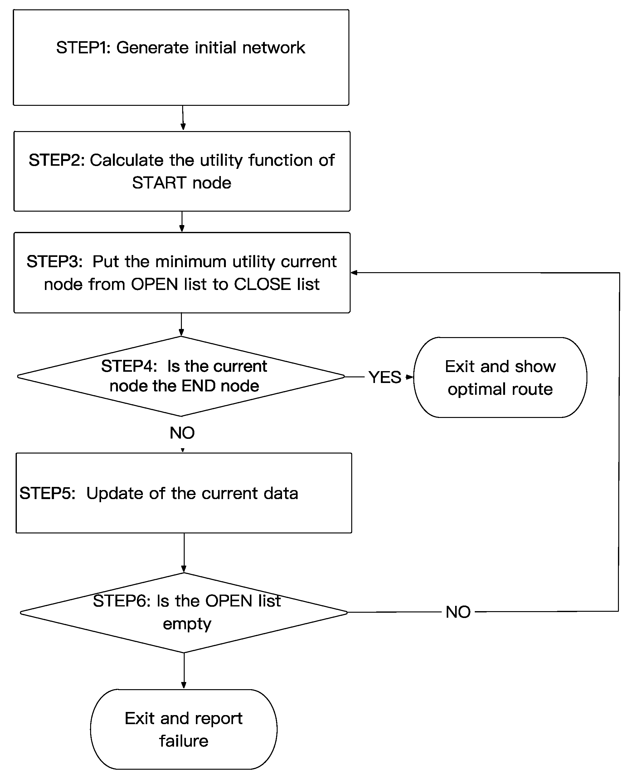
2.1.2. Work Flow
The flow of the algorithm can be seen in Figure 1.
- Step 1
- Initiate two ordered lists called “OPEN” list and “CLOSE” list and generate two nodes called “START” node and “END” node.
- Step 2
- The utility function is calculated by Equation (1) at “START” node and put the “START” node into “OPEN” list.Where, is the estimated value from the “START” node to the “END” node through the current node ; is the actual value from the “START” node to the current node ; is the estimated value from the current node to the “END” node.
- Step 3
- Take out the node of minimum utility from “OPEN” list and mark it as the current node . This node will be saved in “CLOSE” list.
- Step 4
- If and only if the node is not the “END” node, continue the algorithm.
- Step 5
- Evaluate each adjacent node of node and skip the one which has already existed in “CLOSE” list. Then, compute the utility of this node if it is not in “OPEN” list and save it in “OPEN” list. If the node has already existed in “OPEN” list, recalculate the utility of this node and choose the smaller value by comparing the utility with the previous one. Finally, node is assigned as the parent node of the node.
- Step 6
- If “OPEN” list is not empty, back to Step 3. Otherwise, exit and report the failure of route search.
2.2. Basic Concepts of Hesitant Fuzzy Set
2.2.1. Hesitant Fuzzy Set
Hesitant fuzzy set, proposed by [21], is a more general fuzzy set. An HFS is defined in terms of a function that returns a set of membership values for each element in the domain [21].
Definition 1
([21]). A hesitant fuzzy set on is a function that when applied to returns a finite subset of [0,1], which can be represented as the following mathematical symbol:
where is a set of some values in [0,1], denoting the possible membership degrees of the element to the set . For convenience, is named a hesitant fuzzy element (HFE) [22].
Definition 2
([21]). For a hesitant fuzzy set represented by its membership function , we define its complement as follows:
Definition 3
([22]). For an HFE , , is called the score function of , where is the number of elements in and . For two HFEs and , if , then , if , .
2.2.2. The Aggregation Operators for Hesitant Fuzzy Information
Reference [23] proposed an aggregation principle for HFEs:
Definition 4
Based on Definition 4, some new aggregation operators for HFEs were given by [22]:
Definition 5
([22]). Let () be a collection of HFEs, be the weight vector of them, such that and . A generalized hesitant fuzzy weighted averaging (GHFWA) operator is a mapping , and
Definition 6
([22]). Let () be a collection of HFEs, be the weight vector of them, such that and . A generalized hesitant fuzzy weighted geometric (GHFWG) operator is a mapping , such that
2.2.3. Decision Making Based on Hesitant Fuzzy Information
The decision method based on the above definitions can be derived as follows:
- Step 1
- The possible alternative of the attribute provided by decision makers or other sources are denoted by the hesitant fuzzy elements .
- Step 2
- The aggregation operators mentioned above are utilized to obtain the hesitant fuzzy elements ) for the possible alternative ).
- Step 3
- The score values of ) are calculated by Definition 3.
- Step 4
- Choose the optimal alternative by the comparison of .
Example 1.
The vessel, which includes four directions) to navigate, is planed to determine the optimal Arctic route for the following year. Suppose there are three factorsthat affect the decision making—: navigation time;: economic cost;: navigation risk. It should be noted that all of them are of the minimization type. The weight vector of the attributes is.
Then, the optimal route can be determined by using the mentioned method.
- Step 1
- The decision matrix is presented in Table 1, where are in the form of HFEs.
- Step 2
- Two operators, GHFWA and GHFWG, are used to obtain the HFE for the directions ). Take direction as an example and let ; we have
- Step 3
- The score values are calculated by Definition 3, which can be seen in Table 2.
- Step 4
- From Table 2, will be chosen as the optimal direction based on both the GHFWA operator and GHFWG operator where is set as 2.
3. An Improved A* Algorithm (HFS-A*)
In light of the harsh weather conditions in the Arctic region, the primary task for route planning is to identify the obstacles (e.g., sea ice). The Coupled Model Intercomparison Project, phase 5 (CMIP5) provided 39 Global Climate Models (GCMs) to predict sea ice data, from history to 21st century, under different representative concentration pathways (RCPs) [23,24]. Unlike the route planning in other regions, for the current sea ice forecasts in the Arctic region, there exists large uncertainty among these GCMs [25,26], which leads to the uncertainty of the length of the navigation season and the economic risk of exploiting the Arctic routes [27]. Therefore, only treating the shortest distance as the optimal route in the Arctic region is not reasonable; more factors, including the navigation risk, the navigation time, and the economic cost during navigation should be considered. Compared to the traditional A* algorithm, the HFS-A* algorithm is used to tackle the multi-criteria decision-making (MCDM) problem with large uncertainty derived from multi-model outputs and expert knowledge. The improved parts mainly focus on t, the identification of obstacles, and the construction of utility function.
3.1. Navigability of the Arctic Routes
With the impact of global warming, the extent of Arctic sea ice continues to decline [27]. Human’s enthusiasm to explore and develop the Arctic routes are aroused by shorter sailing distance, longer navigation season and increased access to natural resources. There are three criteria related to sea ice conditions for evaluating the navigability in the Arctic area.
Criterion 1 (navigation uncertainty).
Criterion 2 (navigation time).
Criterion 3 (navigation economic cost).
Both sea ice concentration and thickness are considered by computing the Ice Numeral (IN) index from the Arctic Ice Regime Shipping System (AIRSS) provided by the Canada Transport [34,35,36,37]. The Ice Numeral is given by
where is the concentration in tenths of ice type , and is the Ice Multiplier for ice type . Ice type describes the specific stage of development of ice, which is closely related to the ice age. Ice Multipliers, determined by ship class and ice type, are a series of integers, which are used to reflect the impact of sea ice type to the specific vessel. A negative represents the obstacle effect of vessel sailing. Ice types are determined by [34,38], which are presented in Appendix A. For no ice-breaking or ice-strengthening ships, it is navigable when the IN index is larger than zero. Details about vessel type and IM can also be seen in Appendix A.
Additionally, geographical environment, including water depth and channel width, is also a key factor for ships to navigate, which is related to the vessel type and dimension.
Overall, various evaluation criteria will add to the uncertainty of the sea ice navigability projection. In this paper, we take all three criteria into consideration with geographical restriction to make sure the navigability of the Arctic region, in another words, for one region, can be defined as navigable if and only if the criteria mentioned above are all reached.
3.2. Route Planning Criterion 1: Uncertainty of Sea Ice Condition
In this paper, a series of GCMs have been chosen based on their reasonable projections for future sea ice conditions evaluated by literature studies [39,40,41,42] (see Appendix B). In order to obtain the uncertainty of each model, these model outputs were compared with the Pan-Arctic Ice Ocean Modeling and Assimilation System (PIOMAS) estimate data set, which is a reanalysis with good spatial and temporal consistency constrained by the quality of the assimilated observations [43,44,45,46].
Suppose we have GCMs, let each model data-set be , the PIOMAS data set be , then the uncertainty of each model can be obtained as follows:
where, is called cosine similarity, which is a measure of similarity between two non-zero vectors introduced by [47]. represents the bias from the model to the “real state”, which can also be regarded as model uncertainty. When is equal to zero, it represents that the model data sets can well reflect the “real state”, while when is equal to one, the model uncertainty reaches its maximum.
3.3. Route Planning Criterion 2: Time for Navigation on the Arctic Routes
The navigation time for each grid can be depicted as follows:
where, is the distance of each grid, and is the velocity of the vessel on each grid. is the normalization of .
On the Northern Sea Route (NSR), the vessel speed is mainly impacted by sea ice conditions. A h-v curve presented by [48] can reflect, well, the relationship between sea ice thickness and vessel speed. In this h-v curve, the ice resistance and the net thrust of the engine to overcome the ice resistance should both be considered.
- Step 1
- The ice resistance can be presented as follows:where represents the ice porosity factor, is the density difference between ice and water. In this model, these two factors are considered to be constant for simple situations, e.g., when the temperature changes. Variables include the waterline area of the foreship , the Froude number , the length , the parallel midbody length at waterline , the width B, the friction coefficient and the vessel draft . and are mechanical factors of ice found by [49]. The thickness of the brash ice can be determined as follows:Both γ and δ represent the slope angles of the brash ice.The formula can be simplified by an approximation when and [39]:The flare angle ψ mentioned above can be obtained with the bow angles ϕ and α:
- Step 2
- The net thrust can be calculated by the following formula:where is the total thrust, represents the thrust deduction factor, and and are the resistance in ice and in open water respectively.
The effect of vessel speed is approximated by a quadratic factor called bollard pull [50], with the maximum open water speed , and the net thrust can be rewritten as
where v is the vessel speed in the ice, Ke is the bollard pull quality factor, is the propeller diameter and is the actual power delivered.
3.4. Route Planning Criterion 3: Economic Cost for Navigation on the Arctic Routes
The economic cost of navigation on the Arctic routes are consist of four parts, which are capital cost, fuel cost, operation cost, and transit cost:
3.4.1. Model for Capital Cost
Capital cost is related to the price of new ship building or the cost of a ship with loans and depreciations [51]. Generally, the annual capital cost can be computed as follows [52]:
where is a new ship price, eq is the equity, r is the interest rate, and y is the term of loan. The former item is called annual interests, while the latter item is called cash price.
3.4.2. Model for Fuel Cost
Fuel cost is often depicted as the major cost on the marine transportation, which is the largest single cost factor to most related simulations, ranging from 36.7% to 61% [53].
Fuel cost is impacted by the rate of fuel consumption and the price of fuel, which can be descripted as follows:
The fuel consumption of a vessel can be influenced by ship dimensions (e.g., the ship size, hull design, engine profile, speed) and external factors (e.g., sea ice, wind, wave, current, foggy) [51]. The fuel consumption for a specific type of vessel is basically computed by multiplying SFOC (specific fuel oil consumption) (g/kWh), engine power (kw) and sailing hours (h) [54].
Most authors consider speed as the key factor impacting the fuel consumption when the type of a vessel is determined and a simple exponential law based on empirical data are derived: the fuel consumption per unit distance is proportional to the square of the speed [55,56,57], which can be presented as
where and are the fuel consumption rate under the velocity and , respectively. Fuel price is affected by the fluctuation of the global economic market. Low fuel price indicates the depression of global economy, while high fuel price reflects the booming global market.
3.4.3. Model for Operation Cost
Operation cost mainly includes crew cost, insurance cost and maintenance fee which is presented as follows:
1. Crew cost
Crew cost is determined by the vessel type, automation level and numerous other factors [51]. Compared to the open water, the crews in the Arctic region require additional ice navigation experience and the ability to cope with hash weather conditions, which may increase the crew cost [53]. The increased crew cost may come from the higher wage [58] for each member or the larger size of members [59].
2. Maintenance cost
For the purpose of preventing the occurrence of breakdowns and following the scheduled maintenance program, the cost of regular maintenance is needed for vessels.
3. Insurance cost
In face of the risk of Arctic navigation (e.g., collision, engine damage, propeller damage, local hull damage, grounding, etc.) analyzed IN some studies [60,61], maritime insurance is a good tool to mitigate the associated risks, which can be approximately separated into three major components: protection and indemnity (P&I), hull and machinery (H&M), and cargo insurance. The third-party liabilities encountered during the commercial operation of a ship are charged by P&I. H&M covers the cost of damage done to the ship or its equipment. Cargo insurance provides the payment for the damage to the cargo itself [62].
3.4.4. Model for Transit Cost
On the NSR, the transit fee based on vessel type and ice conditions mainly includes ice pilot fee and ice breaking fee and can be given as
These services are mainly provided by the Russian icebreaking service provider, Atomflot, and are compulsively charged subject to the law of the Russian Federation, which is dependent on the vessel type (e.g., the size and the ice-class of a vessel), and the navigation length and pilotage distance [62]. In general, higher ice-classed vessels are charged with lower icebreaking fees.
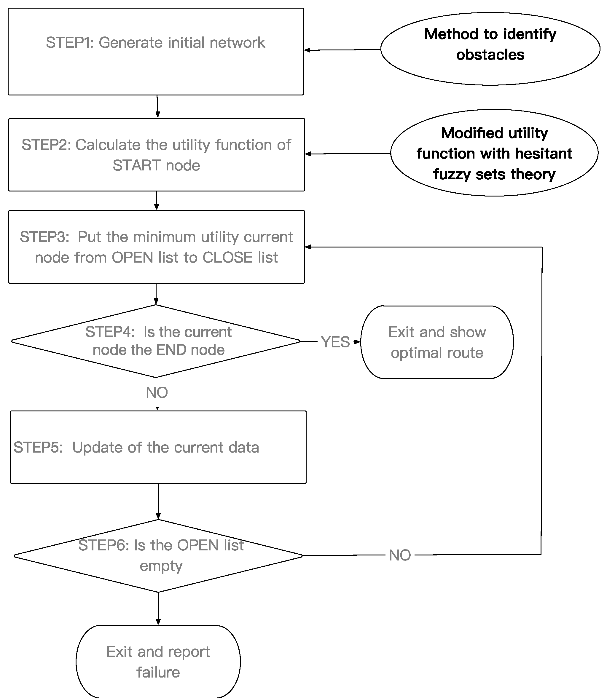
3.5. Work Flow of HFS-A* Algorithm
In this HFS-A* algorithm, the work flow can be seen in Figure 2. The method of obstacle identification has been discussed in Section 3.1 while the modified utility function can be described as follows:
When the current node is determined, the actual cost is equal to the score value , which can be computed by Definition 3.
More specifically, we assume each selected node has three criteria that affect the decision making—: uncertainty of sea ice condition; : navigation time; : navigation economic cost. It should be noted that all of them are of the minimization type. The weight vector of the attributes is .
The heuristic estimated cost function can be approximately evaluated:
where, is the heuristic distance (Manhattan, Euclidean or Chebyshev) from the evaluated node to the END node [63].
Step 1 Map initialization
- Initialize map grid and interpolate the mentioned data into grid.
- Set the “START” node, “END” node, “OPEN” list and “CLOSE” list.
- Find the obstacle nodes in terms of the constrain conditions mentioned in Section 3.1.
Step 2 The construction of utility function
- Each time, compare all the adjacent nodes of the current node bywhere, or , is the HFEs of navigation uncertainty (see Section 3.2), is the HFEs of navigation time (see Section 3.3), and is the HFEs of navigation economic cost (see Appendix D.2).
Step –6 The same as the traditional A* algorithm.
4. Case Study and Conclusion
4.1. Study Area and Data Description
This experiment is to find the optimal route on the Northern Sea Route (NSR) based on the proposed method from Shanghai to Bergen port for an IB-classed 3800TEU container vessel.
Data related to water depth is derived from a product called ETOPO1 provided by the National Geophysical Data Center (NGDC), with a resolution of 1 arc-minute [64]. Data related to AIRSS system can be seen in Appendix A. Data related to sea ice conditions (both sea ice thickness and sea ice concentration) can be seen in Appendix B. Data related to vessel information can be seen in Appendix C. Data related to economic cost can be seen in Appendix D. All the climate model outputs and data related to water depth are interpolated to the grid size of 360 × 120 for the comparison with PIOMAS estimate data set, which the spatial coverage is 45° N to 90N and the temporal resolution is monthly.
4.2. Route Planning by HFS-A* Algorithm
4.2.1. Navigability of the NSR
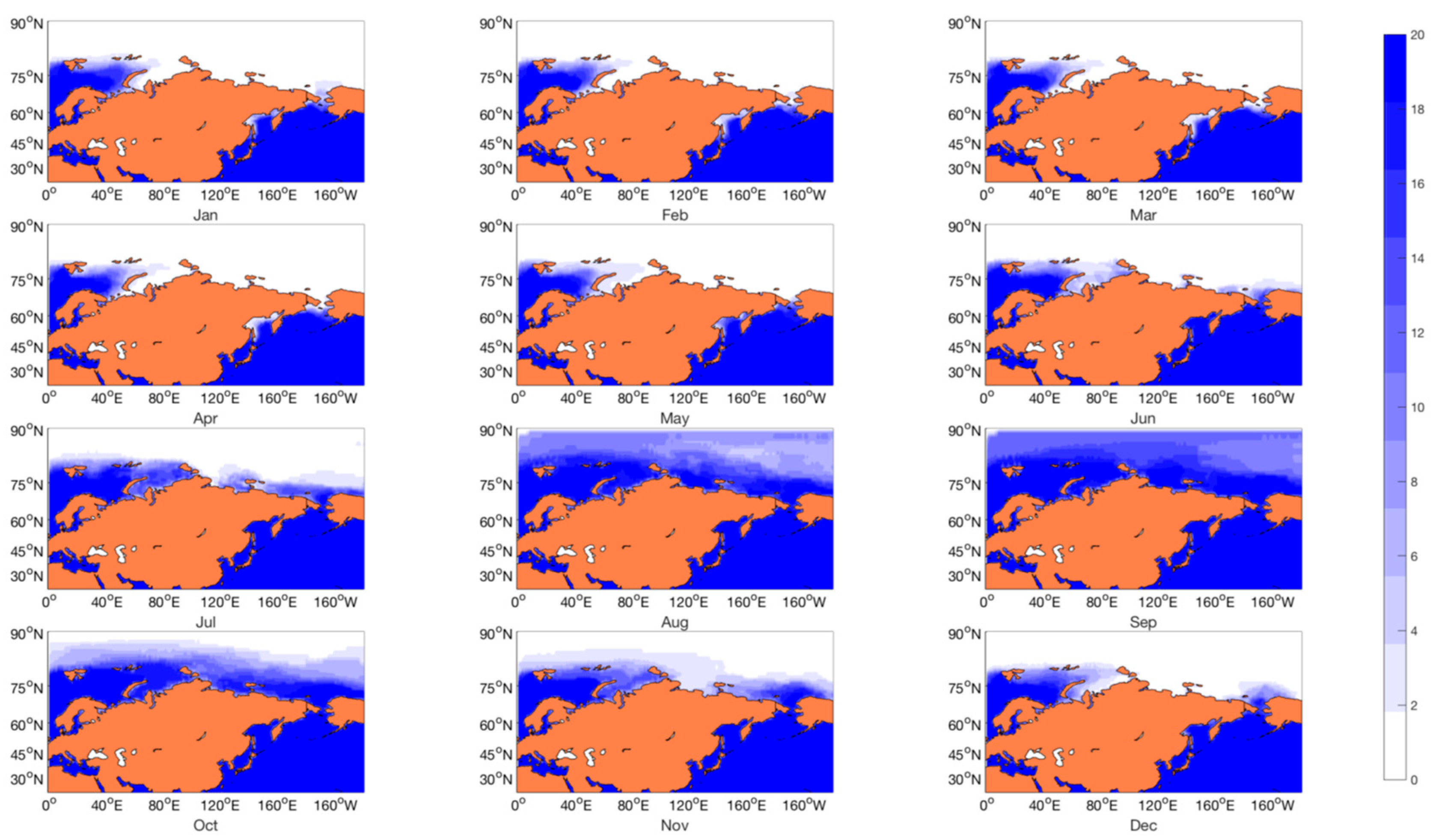
The numerical simulation firstly examines the navigability of the IB-classed 3800 TEU container vessels on the NSR for each month in the year of 2050 (see Figure 3). According to the ensemble model predictions, the open time of the NSR for that vessel to access may last for 3 to 5 months in the year of 2050. Most model outputs show the navigable time starts from August to the October, while merely 2 to 4 models extend the navigable time (from July to November).
4.2.2. Selection of the Aggregation Operators and Route Optimization
Secondly, route planning criteria (uncertainty, time and economic cost) have been calculated based on the models mentioned in Section 3.2, Section 3.3 and Section 3.4, and the results can be seen in Appendix D. These factors can be normalized respectively between 0 and 1, which can be described as:
Thirdly, the optimal routes for IB-classed 3800 TEU container vessels from Shanghai to Bergen port on the NSR in September of 2050 can be found by two kinds of the aggregation operators ( and ), which are used to aggregate the normalized results mentioned above. The detailed results can be seen in Table 3. Compared these two kinds of aggregation operators, the performance of the operators in the route optimization is better than the operators from the view of total sailing distance, sailing time, economic cost and average uncertainty. In the light of the comparison of different for each operator, the performance of the becomes better with the increase, while the performance of the becomes better when decreases. Therefore, the operator has been examined as the best aggregation operator in this numerical study (The weights vectors for this experiment are assigned as 0.4, 0.3, and 0.3 for three criteria).
Finally, the optimal route determined by HFS-A* algorithm with the operator can be seen in Figure 4. Three other routes according to simple single criterion (uncertainty, time, or economic cost) are also drawn in Figure 4. The detailed results can be seen in Table 4, where it can be found that path planning based on a single factor shows a slight advantage in its related aspect, but shows significant disadvantage in any other aspect compared with the optimal route. In other words, the optimal route can better balance these three key factors and show more realistic performance of the proposed route planning algorithm than the other three single factor route planning.
5. Conclusions
The opening of Arctic routes will be no longer a dream in the coming future with climate change; route planning is necessary for vessels to navigation on the Arctic region from different points of view (safe, economic cost, time etc.). This paper presents a modified A* algorithm where the hesitant fuzzy set theory is incorporated for the purpose of solving the MCDM problem in Arctic route planning with large uncertainties originating from multi-climate models and experts’ knowledge. Compared to the traditional A* algorithm, the navigability of the Arctic route is firstly analyzed as a measure to determine the obstacle nodes, and three key factors to vessel navigation, including sailing time, economic cost and risk are overall considered in the HFS-A* algorithm.
A numerical experiment, which is to find the optimal route between Bergen port and Shanghai port on the NSR, is presented to test the performance of the proposed algorithm. Multi-model ensemble forecast displays that the IB-class 3800 TEU container vessels can navigate on the NSR lasting for 3 to 5 months in the year of 2050. Most model outputs show the navigable time starts from August to October, while merely 2 to 4 models extend the navigable time (from July to November). The sensitivity analysis for the aggregation operators examines that the operator has an advantage over other aggregation operators in route optimization, and its performance of integrating the three key factors in route planning is better than the performance of any other single factor.
In this paper, the improvement effects for this new approach have been evaluated theoretically and practically. Theoretically speaking, the simple A* algorithm cannot handle the Arctic path planning problem which has multi-criteria attribution with large uncertainties. Even if we can synthesize the time, economic and uncertainty factors by addition and multiplication, the uncertainties existing in climate model prediction and expert knowledge cannot be portrayed by a simple A* algorithm. Practically speaking, we compared the route planning result of HFS-A* algorithm and single factor route planning result (see Figure 4). It can be found that there is a more realistic performance of the HFS-A* route planning algorithm than compared with the simple A* route planning algorithm. Overall, this new HFS-A* algorithm can be well-applied to the Arctic region and to evaluate the strategic prospects for future Arctic routes.
Author Contributions
Conceptualization, Y.W..; methodology, Y.W.; software, Y.W.; validation, Y.W.; formal analysis, Y.W.; investigation, Y.W.; resources, L.Q.; data curation, L.Q.; writing—original draft preparation, Y.W.; writing—review and editing, R.Z.; supervision, R.Z.; funding acquisition, R.Z., L.Q.
Funding
This work has received funding from the National Natural Science Foundation of China under grant agreement number 51609254 and number 41375002.
Conflicts of Interest
The authors declare no conflicts of interest.
Appendix A

| Ice Type | Characteristic |
|---|---|
| New (Open Water) | Newly formed ice, include ice crystal, grease like ice, crushed ice clusters, etc. These types of ice are just loosely frozen together, can only been seen in the process of floating. The ice thickness is less than 10 cm. |
| Grey | Young ice, has a thickness of 10–15 cm which is lower than that of nilas and is easy to expand and break |
| Grey-white | Young ice has a thickness of 15–30 cm |
| Thin first year 1st stage | One year ice, which the formation time does not exceed one winter, has a thickness of 30–50 cm. |
| Thin first year 2 nd stage | One year ice, which the formation time does not exceed one winter, has a thickness of 50–70 cm. |
| Medium first year | One year ice has a thickness of 70–120 cm |
| Thick first year | One year ice has a thickness of 120–220 cm |
| Second year | Adult ice, which has gone through at least one summer’s melting, has a thickness of 220–250 cm |
| Multiyear | Multiyear ice, which has gone through at least two summers’ melting, has a thickness beyond 250 cm |
Table A2.
Ice Multiplier for ice type [28].
Table A2.
Ice Multiplier for ice type [28].
| Open Water | Grey Ice | Grey White Ice | Thin First Year 1st Stage | Thin FIRST Year 2nd Stage | Medium First Year | Thick First Year | Second Year | Multi Year | |
|---|---|---|---|---|---|---|---|---|---|
| CAC 3 | 2 | 2 | 2 | 2 | 2 | 2 | 2 | 1 | −1 |
| CAC 4 | 2 | 2 | 2 | 2 | 2 | 2 | 1 | −2 | −3 |
| Type A | 2 | 2 | 2 | 2 | 2 | 1 | −1 | −3 | −4 |
| Type B | 2 | 2 | 1 | 1 | 1 | −1 | −2 | −4 | −4 |
| Type C | 2 | 2 | 1 | 1 | −1 | −2 | −3 | −4 | −4 |
| Type D | 2 | 2 | 1 | −1 | −1 | −2 | −3 | −4 | −4 |
| Type E | 2 | 1 | −1 | −1 | −1 | −2 | −3 | −4 | −4 |
Table A3.
Vessel type [28].
Table A3.
Vessel type [28].
| Vessel Type | Description |
|---|---|
| CAC3 | Commercial cargo ship, which can navigate in the area on all kinds of ice types but will escape the area of multiyear ice |
| CAC4 | Commercial cargo ship, which is able to navigate on the area of arbitrary one-year-old ice, while the speed on the area of multiyear ice will be extremely reduced. |
| Type A (IAS, PC6) | Vessel, which can navigate on the area of thick first year ice. |
| Type B (IA, PC7) | Vessel, which can navigate on the area of medium first year ice. |
| Type C (IB) | Vessel, which can navigate on the area of thin first year ice |
| Type D (IC) | Vessel, which can navigate on the area of grey-white ice. |
| Type E (ID) | Vessel, which can navigate on the area of grey-ice. |
Appendix B
Table A4.
Key sources of Global Cliamte Models (GCMs) used in this paper.
| Model | Country | Oceanic Resolution |
|---|---|---|
| ACCESS1.0 | Australia | 1° × 1° L50 |
| ACCESS1.3 | Australia | 1° × 1° L50 |
| BNU-ESM | China | L50 |
| CCSM4 | United States | Nominal 1° (1.125° in longitude, 0.27–0.64° in latitude) L50 |
| CESM1-BGC | United States | Nominal 1° (1.125° in longitude, 0.27–0.64° in latitude) L60 |
| CESM1-CAM5 | United States | Nominal 1° (1.125° in longitude, 0.27–0.64° in latitude) L60 |
| CNRM-CM5 | France | Average 0.7° L42 |
| HADGEM2-CC | United Kingdom | 1.875° × 1.25° |
| MIROC5 | Japan | 0.5–1.4° × 1.4° L50 |
| MPI-ESM-MR | Japan | Approx. 1° × 1° L40 |
Appendix C
Table A5.
Ship dimensions [57].
Table A5.
Ship dimensions [57].
| Vessel Type | IB | ||
|---|---|---|---|
| Deadweight | 50,000 | SFOC | 145.8 |
| Payload | 3800 | engine power | 35,000 |
| Load Factor | 0.65 | Engine load | 0.8 |
| 250 | 24 | ||
| 130 | |||
| 32.2 | |||
| 12 | 0.02 | ||
| 19,600 | 806.5 | ||
| 0.78 | 7.5 | ||
| 6.5 | |||
Appendix D
Appendix D.1. Data Related to Economic Cost
An ordinary 3800 TEU container ship, which usually navigates on the open water, should cost 60 million, the equity is 30%, and the interest rate is 3% with a 20-year loan [65]. Therefore, we can obtain the ordinary capital cost by Equation (23): 10,200 USD/day.
On the NSR, an IB-classed 3800 TEU container ship may have extra building cost due to the principal structure and strength, propulsion system, hull form, etc. [59]. Literature related to extra building cost can be seen in Table A6. From Table A6, the range of the extra building cost for IB-classed vessel is from 5% to 35%.
Suppose is a new ship price, eq is the equity, r is the interest rate and i is the term of loan.
Table A6.
Extra building cost for a commercial ice-classed vessel.
| Ice Class Category Considered | Extra Building Cost | Resource |
|---|---|---|
| CAC3 | +30% | [58] |
| IAS | +20% | [53] |
| IB | +7.5% | [66] |
| PC7 to PC4 1 | +20% | [56] |
| Ice class | +30% | Expert suggestions |
| IA-IAS | +5%–7% | [67] |
| IB | +20%–30% | [59] |
| Ice class | +10%–35% | [68] |
1 According to approximate equivalence of ice class classification systems made by [44], PC6 is equal to 1AS and PC7 is equal to 1A.
The fuel consumption of an ordinary 3800 TEU vessel under the designed speed can be derived based on Table A5: 97.98 ton/day. The current fuel price can be obtained by Bunker Index (www.bunkerindex.com): 450 USD/ton.
It is relatively well-documented in the literature that the fuel consumption of an ice-classed vessel will be more than an ordinary vessel with the same size due to extra weight, bow shape, hull appendages, which increases the frictional resistance [66]. Data related to extra fuel consumption can be seen in Table A7.
Table A7.
Extra fuel consumption rate for a commercial ice-class ship.
| Extra Fuel Consumption Rate | Resource | |
|---|---|---|
| IB | +67% | [59] |
| IAS | +20% | [53] |
| Ice class | +30% | [52] |
| Ice class | +10% | [54] |
| IB | +3% | [65] |
The crew cost for a 3800 TEU ordinary vessel is 2740 USD/day [57]. Data related to extra crew cost can be found in Table A8.
Table A8.
Extra crew cost for a 3800 TEU IB-classed vessel.
| Extra Crew Cost | Resource |
|---|---|
| +0% | Japan Ship owners Association (JSA), 2012 |
| +0% | [65] |
| +10% | [59] |
| +10% | [53] |
| +11%–14% | [58] |
The Maintenance cost of a 3800 TEU ordinary vessel is 1644 USD/day [57]. On the NSR, the IB-classed vessel needs to undergo more challenging operation conditions, which will put extra cost on vessel and equipment (see Table A9).
Table A9.
Extra maintenance cost for a 3800 TEU IB-classed vessel.
| Extra Maintenance Cost | Resource |
|---|---|
| +20% | [53] |
| +20% | [56] |
| +23% | [68] |
| +100% | [59] |
| +100% | [69] |
| +150% | [58] |
The maintenance cost of a 3800 TEU ordinary vessel is 1644 USD/day [57]. Data related to the extra insurance fee of the IB-classed vessel can be seen in Table A10.
Appendix D.2. The Calculation of Economic Cost Based on HFS
The economic cost of an IB-classed 3800 TEU vessel can be derived as follows:
where, the value of each kind of extra cost on the NSR can be determined by 1000 times random sampling from the information mentioned above by Monte Carlo methods using the software of Matlab (Table A11).
Table A11.
Parameters related to the economic cost of an IB-classed 3800 TEU vessel.
| Parameters | Value |
|---|---|
| 0.196 | |
| 0.260 | |
| 0.065 | |
| 0.688 | |
| 0.299 |
From Equations (22)–(27), the economic cost of an IB-classed 3800 TEU vessel for each grid can be obtained as follows:
Specially, the icebreaking fee for each route on the NSR is the same (356,250 USD), so it can be omitted when used as a criterion of route optimization. is the normalization of .
References
- Arctic Council. Arctic Council Arctic Marine Shipping Assessment 2009 Report; Arctic Council: Tromsø, Norway, 2009. [Google Scholar]
- Benjamin, M.R.; Curcio, J.A.; Leonard, J.J.; Newman, P.M. Navigation of Unmanned Marine Vehicles in Accordance with the Rules of the Road. In Proceedings of the 2006 IEEE International Conference on Robotics and Automation, Orlando, FL, USA, 15–19 May 2006. [Google Scholar]
- Szlapczynski, R. A New Method of Ship Routing on Raster Grids, with Turn Penalties and Collision Avoidance. J. Navig. 2006, 59, 27–42. [Google Scholar] [CrossRef]
- Walther, L.; Rizvanolli, A.; Wendebourg, M.; Jahn, C. Modeling and Optimization Algorithms in Ship Weather Routing. Int. J. E-Navig. Marit. Econ. 2016, 4, 31–45. [Google Scholar] [CrossRef]
- Wang, S.; Meng, Q.; Liu, Z. Bunker Consumption Optimization Methods in Shipping: A Critical Review and Extensions. Transp. Res. Part E 2013, 53, 49–62. [Google Scholar] [CrossRef]
- Witt, J.; Dunbabin, M. Go with the Flow: Optimal Path Planning in Coastal Environments. In Proceedings of the Australasian Conference on Robotics & Automation (ACRA), Canberra, Australia, 3–5 December 2008. [Google Scholar]
- Kotovirta, V.; Jalonen, R.; Axell, L.; Riska, K.; Berglund, R. A System for Route Optimization in Ice-Covered Waters. Cold Reg. Sci. Technol. 2009, 55, 52–62. [Google Scholar] [CrossRef]
- Nam, J.H.; Park, I.; Lee, H.J.; Kwon, M.O.; Choi, K.; Seo, Y.K. Simulation of Optimal Arctic Routes Using a Numerical Sea Ice Model Based on an Ice-Coupled Ocean Circulation Method. Int. J. Nav. Archit. Ocean Eng. 2013, 5, 210–226. [Google Scholar] [CrossRef]
- Mulherin, N.D.; Eppler, D.T.; Proshutinsky, T.O.; Farmer, L.D.; Smith, O.P. Development and Results of a Northern Sea Route Transit Model; Cold Regions Research and Engineering Lab: Hanover, NH, USA, 1996. [Google Scholar]
- Choi, Mi.; Chung, H.; Yamaguchi, H.; Nagakawa, K. Arctic Sea Route Path Planning Based on an Uncertain Ice Prediction Model. Cold Reg. Sci. Technol. 2015, 109, 61–69. [Google Scholar] [CrossRef]
- Liu, X.; Sattar, S.; Li, S. Towards an Automatic Ice Navigation Support System in the Arctic Sea. ISPRS Int. J. Geo-Inf. 2016, 5, 36. [Google Scholar] [CrossRef]
- Xia, M.; Xu, Z. Hesitant Fuzzy Information Aggregation in Decision Making. Int. J. Approx. Reason. 2011, 52, 395–407. [Google Scholar] [CrossRef]
- Faizi, S.; Rashid, T.; Sałabun, W.; Zafar, S.; Wątróbski, J. Decision Making with Uncertainty Using Hesitant Fuzzy Sets. Int. J. Fuzzy Syst. 2017, 20, 93–103. [Google Scholar] [CrossRef] [Green Version]
- Zhang, X.; Xu, Z. Novel Distance and Similarity Measures on Hesitant Fuzzy Sets with Applications to Clustering Analysis. J. Intell. Fuzzy Syst. 2015, 28, 2279–2296. [Google Scholar]
- Zhang, Z. Hesitant Fuzzy Power Aggregation Operators and Their Application to Multiple Attribute Group Decision Making. Inf. Sci. 2013, 234, 150–181. [Google Scholar] [CrossRef]
- Rodriguez, R.M.; Martinez, L.; Herrera, F. Hesitant Fuzzy Linguistic Term Sets for Decision Making. IEEE Trans. Fuzzy Syst. 2012, 20, 109–119. [Google Scholar] [CrossRef] [Green Version]
- Song, C.; Xu, Z.; Zhao, H. A Novel Comparison of Probabilistic Hesitant Fuzzy Elements in Multi-Criteria Decision Making. Symmetry 2018, 10, 177. [Google Scholar] [CrossRef]
- Hart, P.E.; Nilsson, N.J.; Raphael, B. A Formal Basis for the Heurist Dennination of Minimum Cost Paths. IEE Trans. Syst. Sci. Cyberetics 1968, 4, 61. [Google Scholar]
- Dijkstra, E.W. A Note on Two Problems in Connexion with Graphs. Numer. Math. 1959, 1, 269–271. [Google Scholar] [CrossRef]
- Zhang, Z.; Schwartz, S.; Wagner, L.; Miller, W. A Greedy Algorithm for Aligning DNA Sequences. J. Comput. Biol. 2000, 7, 203–214. [Google Scholar] [CrossRef] [PubMed]
- Torra, V. Hesitant Fuzzy Sets. Int. J. Intell. Syst. 2010, 25, 529–539. [Google Scholar] [CrossRef]
- Torra, V.; Narukawa, Y. On Hesitant Fuzzy Sets and Decision. In Proceedings of the IEEE International Conference on Fuzzy Systems, Jeju Island, Korea, 20–24 August 2009. [Google Scholar]
- Taylor, K.E.; Stouffer, R.J.; Meehl, G.A. An overview of cmip5 and the experiment design. Bull. Amer. Meteor. Soc. 2012, 93, 485–498. [Google Scholar] [CrossRef]
- Vuuren, D.P.V.; Edmonds, J.A.; Kainuma, M.; Riahi, K.; Weyant, J. A special issue on the rcps. Clim. Chang. 2011, 109. [Google Scholar] [CrossRef]
- Blanchardwrigglesworth, E.; Bitz, C.M. Characteristics of arctic sea-ice thickness variability in gcms. J. Clim. 2014, 27, 8244–8258. [Google Scholar] [CrossRef]
- Melia, N.; Haines, K.; Hawkins, E. Improved arctic sea ice thickness projections using bias-corrected cmip5 simulations. The Cryosphere 2015, 9, 3821–3857. [Google Scholar] [CrossRef]
- Aksenov, Y.; Popova, E.E.; Yool, A.; Nurser, A.G.; Williams, T.D.; Bertino, L.; Bergh, J. On the Future of Arctic Sea Routes: High-Resolution Projections of the Arctic Ocean and Sea Ice. Mar. Policy 2017, 75, 300–317. [Google Scholar] [CrossRef]
- Khon, V.; Mokhov, I. Arctic Climate Changes and Possible Conditions of Arctic Navigation in the 21st Century. Izvestiya Atmos. Ocean. Phys. 2010, 46, 14–20. [Google Scholar] [CrossRef]
- Khon, V.C.; Mokhov, I.I.; Latif, M.; Semenov, V.A.; Park, W. Perspectives of Northern Sea Route and Northwest Passage in the Twenty-First Century. Climat. Chang. 2010, 100, 757–768. [Google Scholar] [CrossRef]
- Khon, V.C.; Mokhov, I.I.; Semenov, V.A. Transit Navigation through Northern Sea Route from Satellite Data and CMIP5 Simulations. Environ. Res. Lett. 2017, 12, 024010. [Google Scholar] [CrossRef]
- Mokhov, I.I.; Khon, V.C.; Prokof’eva, M.A. New Model Estimates of Changes in the Duration of the Navigation Period for the Northern Sea Route in the 21st Century. Dokl. Earth Sci. 2016, 468, 641–645. [Google Scholar] [CrossRef]
- Melia, N.; Haines, K.; Hawkins, E. Sea Ice Decline and 21st Century Trans-Arctic Shipping Routes. Geophys. Res. Lett. 2016, 43, 9720–9728. [Google Scholar] [CrossRef]
- Stephenson, S.R.; Smith, L.C. Influence of Climate Model Variability on Projected Arctic Shipping Futures. Earth’s Future 2015, 3, 331–343. [Google Scholar] [CrossRef]
- CanadaTransport. Arctic Ice Regime Shipping System (AIRSS) Standards; CanadaTransport: Ottawa, ON, Canada, 1998. [Google Scholar]
- Howell, S.E.L.; Yackel, J.J. A Vessel Transit Assessment of Sea Ice Variability in the Western Arctic, 1969–2002: Implications for Ship Navigation. Can. J. Remote Sens. 2004, 30, 205–215. [Google Scholar] [CrossRef]
- Smith, L.C.; Stephenson, S.R. New Trans-Arctic Shipping Routes Navigable by Midcentury. Proc. Natl. Acad. Sci. USA 2013, 110, E1191–E1195. [Google Scholar] [CrossRef]
- Stephenson, S.R.; Smith, L.C.; Brigham, L.W.; Agnew, J.A. Projected 21st-Century Changes to Arctic Marine Access. Clim. Chang. 2013, 118, 885–899. [Google Scholar] [CrossRef]
- Johnston, M.E. Cold Reg. Sci. Technol. Seasonal Changes in the Properties of Fi Rst-Year, Second-Year and Multi-Year Ice. Cold Reg. Sci. Technol. 2017, 141, 36–53. [Google Scholar] [CrossRef]
- Jahn, A.; Sterling, K.; Holland, M.M.; Kay, J.E.; Maslanik, J.A.; Bitz, C.M.; Bailey, D.A.; Stroeve, J.; Hunke, E.C.; Lipscomb, W.H. Late-Twentieth-Century Simulation of Arctic Sea Ice and Ocean Properties in the CCSM4. J. Clim. 2012, 25, 1431–1452. [Google Scholar] [CrossRef]
- Liu, J.; Song, M.; Horton, R.M.; Hu, Y. Reducing Spread in Climate Model Projections of a September Ice-Free Arctic. Proc. Natl. Acad. Sci. USA 2013, 110, 12571–12576. [Google Scholar] [CrossRef]
- Massonnet, F.; Fichefet, T.; Goosse, H.; Vancoppenolle, M.; Mathiot, P.; König Beatty, C. On the Influence of Model Physics on Simulations of Arctic and Antarctic Sea Ice. Cryosphere 2011, 5, 687–699. [Google Scholar] [CrossRef]
- Vavrus, S.J.; Holland, M.M.; Jahn, A.; Bailey, D.A.; Blazey, B.A. Twenty-First-Century Arctic Climate Change in CCSM4. J. Clim. 2012, 25, 2696–2710. [Google Scholar] [CrossRef]
- Laxon, S.W.; Giles, K.A.; Ridout, A.L.; Wingham, D.J.; Willatt, R.; Cullen, R.; Kwok, R.; Schweiger, A.; Zhang, J.; Haas, C.; et al. CryoSat-2 Estimates of Arctic Sea Ice Thickness and Volume. Geophys. Res. Lett. 2013, 40, 732–737. [Google Scholar] [CrossRef]
- Lindsay, R. New Unified Sea Ice Thickness Climate Data Record. Eos 2010, 91, 405–406. [Google Scholar] [CrossRef]
- Schweiger, A.; Lindsay, R.; Zhang, J.; Steele, M.; Stern, H.; Kwok, R. Uncertainty in Modeled Arctic Sea Ice Volume. J. Geophys. Res. Oceans 2011. [Google Scholar] [CrossRef]
- Stroeve, J.; Barrett, A.; Serreze, M.; Schweiger, A. Using Records from Submarine, Aircraft and Satellites to Evaluate Climate Model Simulations of Arctic Sea Ice Thickness. Cryosphere 2014, 8, 1839–1854. [Google Scholar] [CrossRef]
- Salton, G.; McGill, M.J. Introduction to Modern Information Retrieval; McGraw-Hill: New York, NY, USA.
- Juva, M.; Riska, K. On the Power Requirement in the Finnish-Swedish Ice Class Rules; Research Report No.47; Helsinki University of Technology, Ship Laboratory: Espoo, Finland, 2002. [Google Scholar]
- Kujala, P.; Sundell, T. Performance of Ice-Strengthened Ships in the Northern Baltic Sea in Winter 1991; Helsinki University of Technology, Laboratory of Naval Architecture and Marine Engineering: Espoo, Finland, 1992. [Google Scholar]
- Riska, K.; Wilhelmson, M.; Englund, K.; Leiviskä, T. Performance of Merchant Vessels in the Baltic; Research report No. 52; Helsinki University of Technology, Ship Laboratory, Winter Navigation Research Board: Espoo, Finland, 1997. [Google Scholar]
- Wijnolst, N.; Wergeland, T. Shipping Innovation; IOS Press: Amsterdam, The Netheriands, 2009. [Google Scholar]
- Zhang, Y.; Meng, Q.; Ng, S.H. Shipping Efficiency Comparison between Northern Sea Route and the Conventional Asia-Europe Shipping Route via Suez Canal. J. Transp. Geogr. 2016, 57, 241–249. [Google Scholar] [CrossRef]
- Lasserre, F. Case Studies of Shipping along Arctic Routes. Analysis and Profitability Perspectives for the Container Sector. Transp. Res. Part A Policy Pract. 2014, 66, 144–161. [Google Scholar] [CrossRef]
- Furuichi, M. Economic Feasibility of Finished Vehicle and Container Transport by NSR/SCR-Combined Shipping between East Asia and Northwest Europe. In Proceedings of the IAME 2014 Conference, Norfolk, VA, USA, 15–18 July 2014. [Google Scholar]
- Furuichi, M. Cost Analysis of the Northern Sea Route (NSR) and the Conventional Route Shipping. In Proceedings of the IAME 2013 Conference 2013, Marseille, France, 3–5 July 2013; Volume 13. [Google Scholar]
- Schøyen, H.; Bråthen, S. The Northern Sea Route versus the Suez Canal: Cases from Bulk Shipping. J. Transp. Geogr. 2011, 19, 977–983. [Google Scholar] [CrossRef]
- Xu, H.; Yin, Z.; Jia, D.; Jin, F.; Ouyang, H. The Potential Seasonal Alternative of Asia-Europe Container Service via Northern Sea Route under the Arctic Sea Ice Retreat. Marit. Policy Manag. 2011, 38, 541–560. [Google Scholar] [CrossRef]
- Somanathan, S.; Flynn, P.; Szymanski, J. The Northwest Passage: A Simulation. Transp. Res. Part A Policy Pract. 2009, 43, 127–135. [Google Scholar] [CrossRef]
- Liu, M.; Kronbak, J. The Potential Economic Viability of Using the Northern Sea Route (NSR) as an Alternative Route between Asia and Europe. J. Transp. Geogr. 2010, 18, 434–444. [Google Scholar] [CrossRef]
- Goerlandt, F.; Montewka, J. A Framework for Risk Analysis of Maritime Transportation Systems: A Case Study for Oil Spill from Tankers in a Ship–Ship Collision. Saf. Sci. 2015, 76, 42–66. [Google Scholar] [CrossRef]
- Valdez Banda, O.A.; Goerlandt, F.; Montewka, J.; Kujala, P. A Risk Analysis of Winter Navigation in Finnish Sea Areas. Accid. Anal. Prev. 2015, 79, 100–116. [Google Scholar] [CrossRef]
- Kiiski, T. Feasibility of Commercial Cargo Shipping Along the Northern Sea Route; University of Turku: Turku, Finland, 2017. [Google Scholar]
- Duchoň, F.; Babinec, A.; Kajan, M.; Beňo, P.; Florek, M.; Fico, T.; Jurišica, L. Path Planning with Modified A Star Algorithm for a Mobile Robot. Procedia Eng. 2014, 96, 59–69. [Google Scholar] [CrossRef]
- Amante, C.; Eakins, B.W. ETOPO1 1 Arc-Minute Global Relief Model: Procedures, Data Sources and Analysis; NOAA Technical Memorandum NESDIS NGDC-24; National Oceanic and Atmospheric Administration: Boulder, CO, USA, 2009.
- Omre, A. An Economic Transport System of the next Generation Integrating the Northern and Southern Passages. Master’s Thesis, Institutt for marin teknikk, Trondheim, Norway, 2012. [Google Scholar]
- Erikstad, S.O.; Ehlers, S. Decision Support Framework for Exploiting Northern Sea Route Transport Opportunities. Ship Technol. Res. 2012, 59, 34–42. [Google Scholar] [CrossRef]
- Pruyn, J.F.J. Will the Northern Sea Route Ever Be a Viable Alternative? Marit. Policy Manag. 2016, 43, 661–675. [Google Scholar] [CrossRef]
- Ostreng, W.; Eger, K.M.; Fløistad, B.; Jørgensen-Dahl, A.; Lothe, L.; Mejlænder-Larsen, M.; Wergeland, T. Shipping in Arctic Waters: A Comparison of the Northeast, Northwest and Trans Polar Passages; Springer: Chichester, UK, 2013. [Google Scholar]
- Verny, J.; Grigentin, C. Container Shipping on the Northern Sea Route. Int. J. Prod. Econ. 2009, 122, 107–117. [Google Scholar] [CrossRef]
- Srinath, B.N. Arctic Shipping—Commercial Viability of the Arctic Sea Routes. Master’s Thesis, Delft University of Technology, Delft, The Netherlands, 2010. [Google Scholar]
- Gritsenko, D.; Kiiski, T. A Review of Russian Ice-Breaking Tariff Policy on the Northern Sea Route 1991–2014. Polar Rec. 2016, 52, 144–158. [Google Scholar] [CrossRef]
Figure 1.
Work flow of the traditional A* algorithm.

Figure 2.
Work flow of the HFS-A* algorithm.

Figure 3.
The navigability of IB-classed 3800 TEU container vessels on the NSR for each month in the year of 2050 based on multi-models. (The color of orange in the map reflects the geographic information, the white color represents the area that cannot access during that month, different blue colors reflect different amount of the models that give the navigable prediction for each grid during that month.).

Figure 4.
Route optimization for IB-classed 3800 TEU container vessels on the NSR from Shanghai to Bergen port in September of 2050 by HFS-A* algorithm. (The red line represents the route planning based on navigation uncertainty, the blue line based on the navigation time, the yellow line based on navigation economic cost, the dark line represents the optimal route integrated of these three criteria by the operator.)

Table 1.
Hesitant fuzzy decision matrix.
| (0.1, 0.3, 0.5) | (0.2, 0.6, 0.8) | (0.3, 0.4, 0.5) | |
| (0.2, 0.4, 0.7) | (0.1, 0.2, 0.4) | (0.3, 0.4, 0.6) | |
| (0.3, 0.5, 0.6) | (0.2, 0.4, 0.5) | (0.3, 0.5, 0.7) | |
| (0.3, 0.5, 0.6) | (0.4, 0.5, 0.6) | (0.2, 0.5, 0.6) |
Table 2.
Score values obtained by the GHFWA operator and GHFWG operator and the rankings of alternatives ().
Table 2.
Score values obtained by the GHFWA operator and GHFWG operator and the rankings of alternatives ().
| Ranking | |||||
|---|---|---|---|---|---|
| GHFWA2 | 0.4777 | 0.3993 | 0.4644 | 0.4887 | |
| GHFWG2 | 0.3649 | 0.3052 | 0.3052 | 0.3052 |
Table 3.
Results of route optimization for IB-classed 3800 TEU container vessels on the NSR from Shanghai to Bergen port in September of 2050 with different aggregation operators based on HFS-A* algorithm.
Table 3.
Results of route optimization for IB-classed 3800 TEU container vessels on the NSR from Shanghai to Bergen port in September of 2050 with different aggregation operators based on HFS-A* algorithm.
| Distance (Nautical Miles) | Sailing Time (day) | Economic Cost (Million USD) | Uncertainty (Mean) | |
|---|---|---|---|---|
| GHFHA1 | 9900 | 25.99 | 1.20 | 0.5105 |
| GHFHA2 | 10,110 | 26.53 | 1.21 | 0.5104 |
| GHFHA6 | 10,142 | 26.98 | 1.23 | 0.5102 |
| GHFHG1 | 8451 | 22.61 | 1.08 | 0.4700 |
| GHFHG2 | 8513 | 22.78 | 1.09 | 0.4704 |
| GHFHG6 | 8341 | 22.33 | 1.07 | 0.4901 |
Table 4.
Results of route optimization for IB-classed 3800 TEU container vessels on the NSR from Shanghai to Bergen port in September of 2050 based on HFS-A* algorithm and simple A* algorithm (The percentages in brackets are compared with the values in GHFHG1).
Table 4.
Results of route optimization for IB-classed 3800 TEU container vessels on the NSR from Shanghai to Bergen port in September of 2050 based on HFS-A* algorithm and simple A* algorithm (The percentages in brackets are compared with the values in GHFHG1).
| Distance (Nautical Miles) | Sailing Time (Day) | Economic Cost (Million USD) | Uncertainty (Mean) | |
|---|---|---|---|---|
| GHFHG1 | 8451 | 22.61 | 1.08 | 0.4700 |
| Uncertainty | 10,674 (+26.0) | 27.87 (+23.3%) | 1.26 (+16.7%) | 0.4404 (-6.3%) |
| Time | 8603 (+1.7%) | 21.97 (−2.8%) | 1.07 (-0.9%) | 0.5148 (+9.5%) |
| Economic cost | 8167 (−3.4%) | 21.07 (−6.8%) | 1.04 (-3.7%) | 0.5516 (+17.4%) |
© 2018 by the authors. Licensee MDPI, Basel, Switzerland. This article is an open access article distributed under the terms and conditions of the Creative Commons Attribution (CC BY) license (http://creativecommons.org/licenses/by/4.0/).
Share and Cite
MDPI and ACS Style
Wang, Y.; Zhang, R.; Qian, L. An Improved A* Algorithm Based on Hesitant Fuzzy Set Theory for Multi-Criteria Arctic Route Planning. Symmetry 2018, 10, 765. https://0-doi-org.brum.beds.ac.uk/10.3390/sym10120765
AMA Style
Wang Y, Zhang R, Qian L. An Improved A* Algorithm Based on Hesitant Fuzzy Set Theory for Multi-Criteria Arctic Route Planning. Symmetry. 2018; 10(12):765. https://0-doi-org.brum.beds.ac.uk/10.3390/sym10120765
Chicago/Turabian StyleWang, Yangjun, Ren Zhang, and Longxia Qian. 2018. "An Improved A* Algorithm Based on Hesitant Fuzzy Set Theory for Multi-Criteria Arctic Route Planning" Symmetry 10, no. 12: 765. https://0-doi-org.brum.beds.ac.uk/10.3390/sym10120765
Note that from the first issue of 2016, this journal uses article numbers instead of page numbers. See further details here.