SDAE-BP Based Octane Number Soft Sensor Using Near-infrared Spectroscopy in Gasoline Blending Process


1
School of Optical-Electrical and Computer Engineering, University of Shanghai for Science and Technology, Shanghai 200093, China
2
School of Mechanical Engineering, University of Shanghai for Science and Technology, Shanghai 200093, China
3
School of Energy and Power Engineering, University of Shanghai for Science and Technology, Shanghai 200093, China
*
Author to whom correspondence should be addressed.
Symmetry 2018, 10(12), 770; https://0-doi-org.brum.beds.ac.uk/10.3390/sym10120770
Submission received: 20 November 2018
/
Accepted: 17 December 2018
/
Published: 18 December 2018
Abstract
:As the most important properties in the gasoline blending process, octane number is difficult to be measured in real time. To address this problem, a novel deep learning based soft sensor strategy, by using the near-infrared (NIR) spectroscopy obtained in the gasoline blending process, is proposed. First, as a network structure with hidden layer as symmetry axis, input layer and output layer as symmetric, the denosing auto-encoder (DAE) realizes the advanced expression of input. Additionally, the stacked DAE (SDAE) is trained based on unlabeled NIR and the weights in each DAE is recorded. Then, the recorded weights are used as the initial parameters of back propagation (BP) with the reason that the SDAE trained initial weights can avoid local minimums and realizes accelerate convergence, and the soft sensor model is achieved with labeled NIR data. Finally, the achieved soft sensor model is used to estimate the real time octane number. The performance of the method is demonstrated through the NIR dataset of gasoline, which was collected from a real gasoline blending process. Compared with PCA-BP (the dimension of datasets of BP reduced by principal component analysis) soft sensor model, the prediction accuracy was improved from 86.4% of PCA-BP to 94.8%, and the training time decreased from 20.1 s to 16.9 s. Therefore, SDAE-BP is proposed as a novel method for rapid and efficient determination of octane number in the gasoline blending process.
1. Introduction
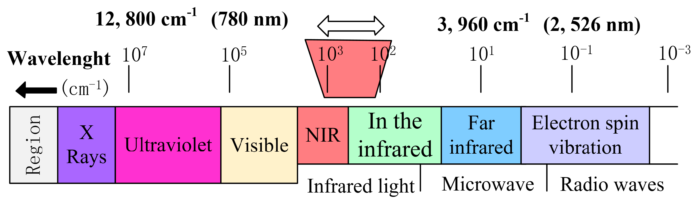
Since the gasoline engine became vehicle power in the 19th century, the importance of gasoline has been increasing. In industry, gasoline is produced by fractionation and heavy-distillation of crude oil. Fractionated gasoline usually has a low octane number. In order to obtain better performance of gasoline, high-octane components are usually added to gasoline for blending. The most important indicator of gasoline during blending is the octane number, which reflects the performance of the gasoline. The higher the octane number is, the better antiknock performance it possesses. In the process of online gasoline blending, NIR spectrometers are often used to quickly detect the octane number through the appropriate soft sensor model [1] since it captures a wealth of information [2]. Near-infrared light refers to electromagnetic waves with wavelengths between the visible and mid-infrared ranges of 780 nm to 2526 nm, as shown in Figure 1.
Soft sensor technology has gradually developed in these days [3]. It can be divided into two categories: The first principles method, which is practical under the laws of variable physics and explicit interpretation, is difficult to build accurate mathematical models for complex industrial processes [4]. Therefore, another modeling method: A data-driven modeling method came into being. This model has always been regarded as a black box model. There is no need to study the internal laws, but the most sufficient sample data matters [5]. Research on data-driven soft sensing of octane has been carried out for decades and many excellent methods have been proposed. For instance, Andrade JM et al. [6] put partial least-squares (PLS) in the modeling of soft sensor for octane. Creton B et al. [7] proposed a quantitative structure property relationship (QSPR) method to predict the octane. Yao X et al. [8] used the least square support vector machine (LSSVM) for octane soft sensor. Wang T et al. [9] put forward a octane soft sensing method of backward interval partial least squares (BiPLS). They all used the date-driven methods to predict the octane, but these methods are slightly inferior in accuracy and timeliness.
Meanwhile, researches showed that the neural network soft-sensing model is considerably splendid in addressing the nonlinear relationship between the input and output variables [10,11]. Gao J et al. [12] used the neural network to predict the octane number and good prediction results have been achieved. This indicates that neural networks have potential for further research in predicting regression. The disadvantage is that the neural network is easy to overfit, and the generalization ability is not quite excellent. Some studies [13,14,15,16] presented the improvement method, for example, the adaptive method, fuzzy neural network, and so on. Moreover, considering that deep learning is superior to other nonlinear methods, it has become a research hotspot to use deep learning to compensate for the shortcomings of ordinary neural networks soft sensor.
As an unsupervised feature learning neural network, deep learning can get a very complex nonlinear relationship between the input and output through a series of transformations without prior knowledge. The advantage of deep learning lies in the adjustment of its structure, optimization of weights, and strong fitting ability and quick response. The existing methods for deep learning include convolutional neural networks (CNN), recurrent neural networks (RNN), deep belief networks (DBN), generative adversarial networks (GAN), and stacked auto-encoding networks (SAE). For instance, to extract deeper features, Lee et al. [17] introduced sparsity into auto-encoding networks based on the nature of the human visual cortex v2, which proved that the sparse performance enables auto-encoding networks to learn deeper features. To extract higher level abstract features, Vincent et al. [18] proposed a denoising auto-encoder (DAE), which also indicated that DAE should be able to efficiently reconstruct the original data from missing or noise-containing input data. Rifai et al. [19] further improved the robustness of feature extraction via proposed a contractive auto-encoder (CAE) that can generate local spatial contraction. CAE uses the Frobenius norm of the Jacobian matrix in the loss function of the auto-encoding network as a penalty. To solve the phenomenon of over-fitting caused by the synergetic action between neurons in the network, Hinton et al. [20] proposed the dropout technique to make a certain proportion of hidden layer nodes temporarily fail in the process of neural network training, aiming at the deep network training of small sample data sets, and the phenomenon of over-fitting is reduced significantly.
Based on deep learning technology, this study establishes a soft-sensing model of octane number by using NIR data. In the proposed method, the stacked denosing auto-encoder (SDAE) is trained based on unlabeled NIR and the weights in each DAE is recorded with the high level feature extraction and reduction of input data. Then, the recorded weights are used as the initial parameters of back propagation (BP) with the reason that the SDAE trained initial weights can avoid local minimums and realize accelerate convergence, and the soft sensor model is achieved with labeled NIR data. In the training process, the gradient descent strategy is applied to update parameter and L2 regularization tragic, which can avoid overfitting, and is used to optimize the loss function. Finally, the achieved soft sensor model is used to estimate the real time octane number.
The structure of this paper is as follows: Section 1 summarizes the development of soft-sensing and deep learning; Section 2 introduces SDAE deep neural network; Section 3 proposes SDAE-BP model and summarizes gradient descent methods; Section 4 shows the research results of octane number soft sensing; and finally, conclusions are drawn in Section 5.
2. SDAE Neural Network
2.1. Auto-Encoder
As an unsupervised learning method, auto-encoding (AE) is a three-layer neural network model that includes a data input layer, a hidden layer, and an output target reconstruction layer. As a network structure with then hidden layer as symmetry axis, the input layer and output layer are symmetric, the AE realizes the advanced expression of input. The structure is shown in Figure 2.
As shown in Figure 2, the input of AE is , the hidden layer in the middle is , and the network output is . The special nature of the auto-encoding network is that the number of input neurons and the number of output neurons are equal. Therefore, is considered as a reconstruction representation of . From the input layer to the hidden layer is called the encoding process, so that the hidden layer gets a more advanced input feature expression, and the encoding function is ; the hidden layer to the output layer is called the decoding process, and the decoding function is .
From the i-th layer mapping to the (i + 1)-th layer, the neural network needs the activation function to provide the learning ability for the nonlinear mapping. The sigmoid function is generally used as the activation function.
Moreover, in the AE network, the number of neurons in the hidden layer is less than the input layer, so the encoding process is to compress the data and the hidden layer has a higher level of expression, which is equivalent to the dimension reduction of the PCA. The encoding function from to is:
in the formula:
—Bias term. The default value is 1;
—Activation function (sigmoid);
—n × m weight matrix of input to hidden layer;
—Parameters of the scalar, .
From the hidden layer y to the reconstructed output layer , this mapping process is called decoding and the decoding function is :
in the formula:
—Bias terms;
—m × n weight matrix from the hidden layer to the output layer.
The output of AE is a reconstruction expression of input, and the error is used to describe the reconstruction result. The relationship between the output and the input is shown as follows:
2.2. Denosing Auto-Encoder
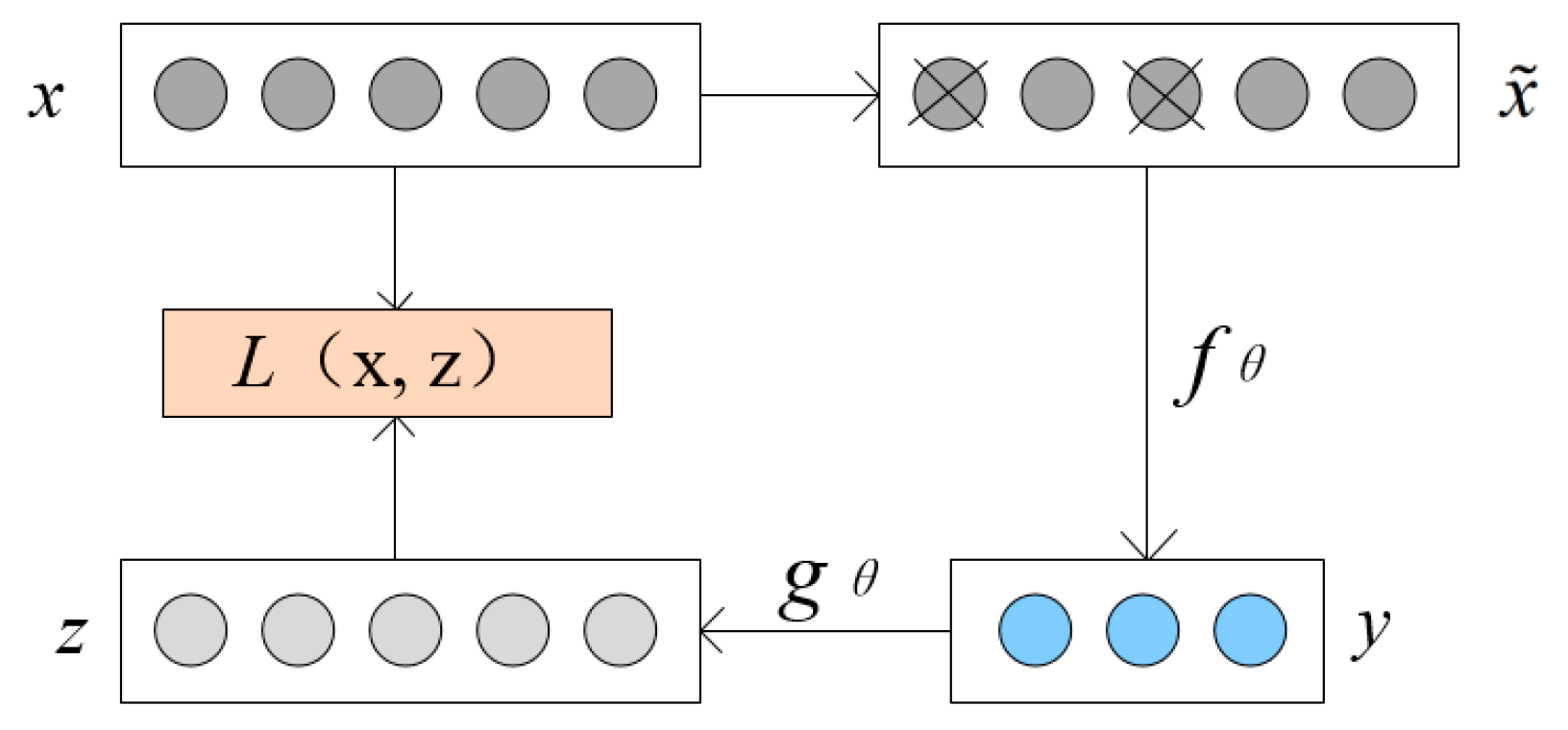
In the encoding process of AE, in order to simulate the effect of the transformation, the nonlinear W needs to set at a very small value; at the same time, for the decoding process, a very large is needed to effectively reconfigure the original input , these settings have increased the convergence rate empirically. However, it is difficult to produce particularly large weights with the general optimization algorithm. As the research progresses, scientists have found that randomly changing the values of some dimensions of the input data to 0 can enhance the generalization and refactoring capabilities of the mode and restore a more expressive [21]. In special cases, even up to half of the dimensions of are set to 0. This practice is called adding noise and this is the prototype of the denosing auto-encoder (DAE). The structure of DAE is shown in Figure 3. The method for adding noise is to add a certain proportion of Gaussian noise ( satisfied ) to the input data , and control the proportion of added noise by setting different values. The noises are input into the auto-encoder, and the error between the output date and the original input were calculated. The stochastic gradient descent algorithm [22] is used to adjust the weight to minimize the error and to optimize the parameter .
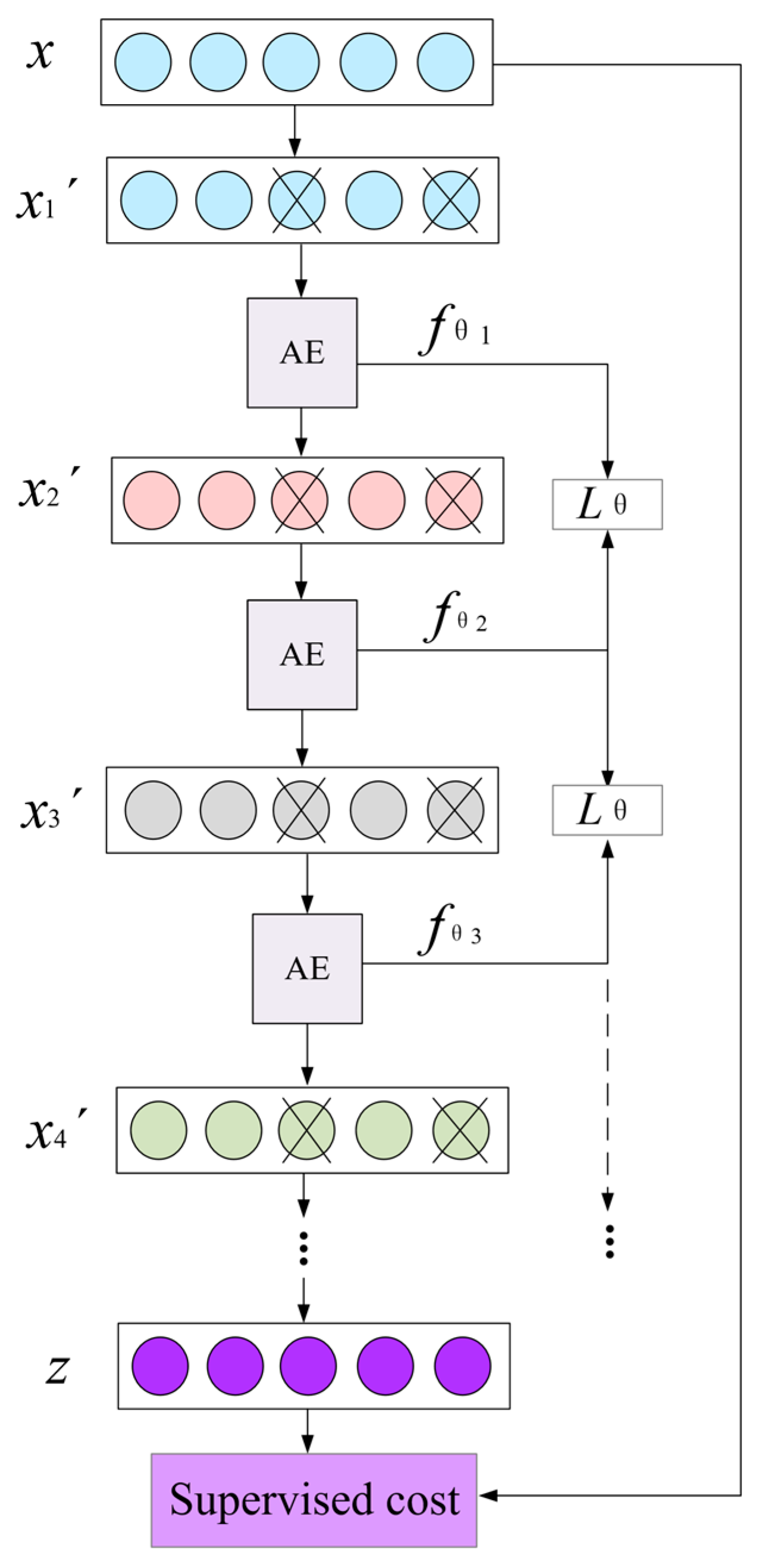
When learning big data, the coding capacity of three-layer neural network of DAE is limited, and the training effect can not meet the demand. In order to learn a more effective feature representation, multiple DAEs are stacked together to form a new deep learning framework: Stack denoising auto-encoder (SDAE), which was proposed by Hitton in 2006 [23]. SDAE has good performance in data reduction, classification, and clustering, and it uses layer-by-layer unsupervised greedy training. The SDAE structure is shown in Figure 4.
The figure reflected that SDAE is formed by superimposing multiple DAEs. In the training process, the input is after adding noise to the input data , and the function of the first AE that mapping to the hidden layer is expressed as . The reconstructed output of the first AE plus noise is , which is the input data of the second AE. The function of the hidden layer of the second AE is expressed as . The , which represents the loss function between two DAEs, is calculated by the function expression of two AEs hidden layers in order to correct the weights of the hidden layer of the previous AE. Then, continue the above process until all AE have completed training. Then, the SDAE network is regarded as a whole, and the error is calculated by using the original input and the reconstruction of the final output. By constraining the reconstruction error, the weight value can satisfy the mapping relation between the input and the output.
3. SDAE-BP Soft Sensor Model
In this study, to realize the soft sensor of octane number based on NIR in gasoline blending process, a novel SDAE based soft sensor strategy is proposed, in which weights trained by SDAE will be assigned to BP as its initial parameters with the reason that the SDAE trained initial weights can avoid local minimums and realize accelerate convergence, then a soft sensor model will be established. The details are as follows:
3.1. BP Neural Network
BP is a kind of neural network with positive inflow of data and back propagation of errors to each layer of the network to adjust the weights and other parameters. Just like AE, the BP network structure also has three layers: Input layer with neurons, hidden layer with m neurons, and output layer with k neurons.
The input of the weighted hidden layer is:
in the formula:
—Weight;
—Bias;
—Number of neurons in the input layer;
—Number of neurons in the hidden layer.
The output of the hidden layer is mapped by the activation function:
The output of output layer is:
in the formula:
—Number of neurons in the output layer.
Calculate the error between output and expected output :
The weight initialization of the BP neural network is usually implemented by Nguyen-Widrow [24] algorithm, and it obeys the Gaussian distribution. The initial weights and bias randomly appear in [0, 1] or [−1, 1], the experiments showed that the BP soft sensor model is easy to get into the local minimums and the speed of convergence is slow. Based on the shortage of BP, this study proposed the SDAE network to initialize the parameters of BP to achieve stable training performance.
3.2. Gradient Descent
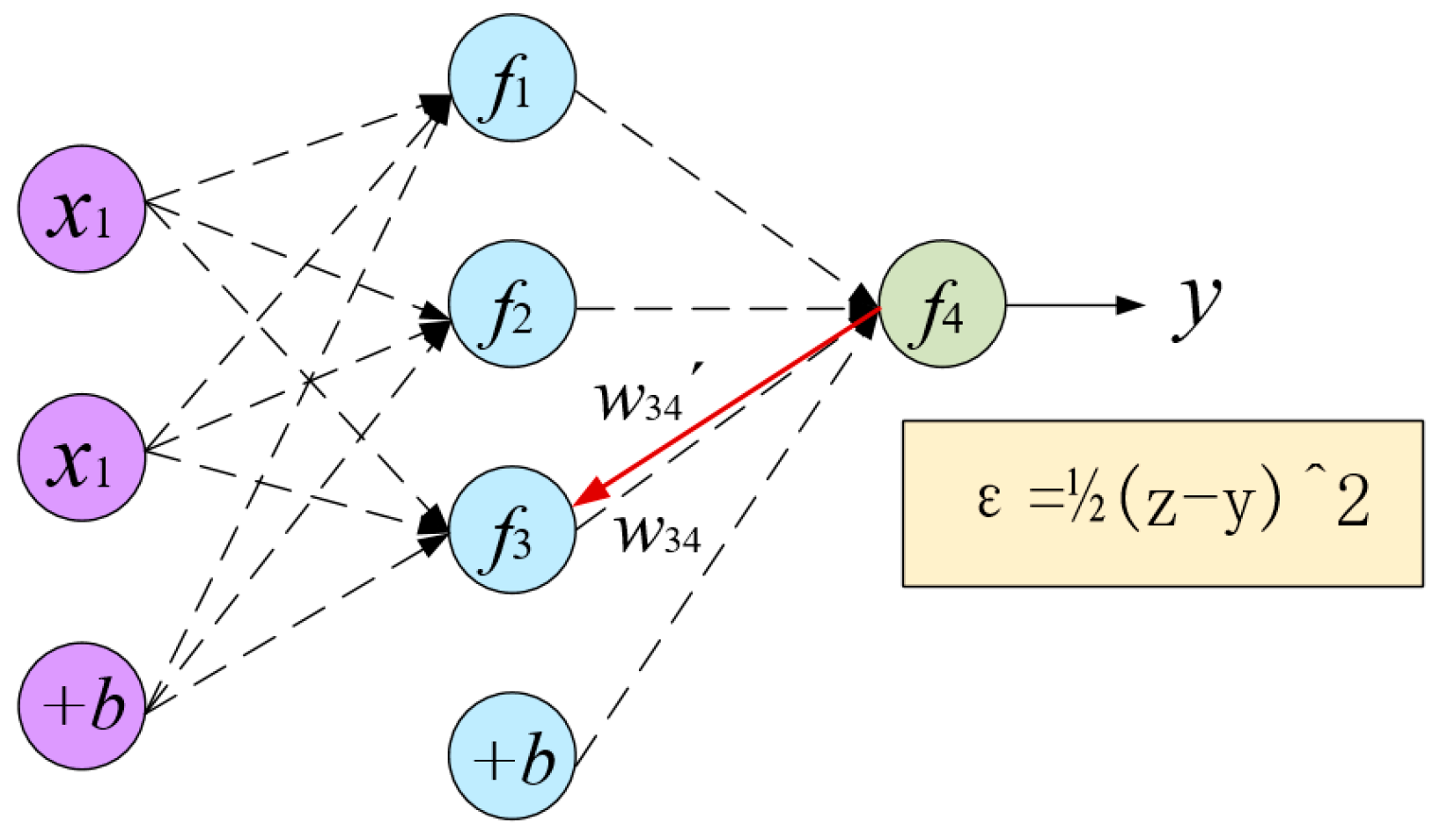
Gradient descent is in fact a partial derivative of the loss function to update the parameters of the model, as shown in Figure 5.
Figure 5 revealed that the data is mapped from the input layer to the output layer, the actual output of the network is , and the expected output is . In order to optimize the error of neural network output and expected output, each layer parameter should be adjusted by gradient descent. Take node in the figure as an example, the original weight is mapped from hidden layer to output layer. The new weight is the result of the original weight minus the partial derivative of the output layer to the weight. The weight update formula is:
in the formula:
—Learning rate, constraints to control fitting ability;
—Mean square error.
There are two main methods for gradient descent: stochastic gradient descent and batch gradient descent [25].
3.3. Optimization Term
3.3.1. Optimization of Loss Function
According to the principle of statistics, we assume that the error (in Equations (3) and (7)) is based on Gaussian distribution: , so the error likelihood function is , and its expansions are: .
In the error logarithmic likelihood formula, we can get the objective function. The construction of the loss function is to make the error logarithmic likelihood result as large as possible, so the loss function will be:
where, the is actually the least square method, During the training process, the loss function should be continuously minimized to update the parameters of the model.
To avoid the problem of decreasing the learning rate of the objective function, we use cross-entropy [26] to optimize the objective function. At this time, the loss function is settled:
To further optimize the loss function between the input and reconstructed output of SDAE, a more refined model should consider overfitting problems by minimizing the variance and deviation of training error and generalization error. We applied the L2 regularization tragic and the optimized loss function at this time is expressed as:
in the formula:
—Regularization parameters. The latter part of the formula is a regularization weight attenuation term to prevent over-fitting;
—Number of layers;
—Number of neural nodes in the l-th layer without bias terms;
—Input of SDAE;
—Reconstructive output of SDAE.
3.3.2. Determination of Gradient Descent Method
There are generally two methods for gradient descent: Stochastic gradient descent and batch gradient descent.
The first step of the stochastic gradient descent method is that only one randomized training sample is selected to calculate the gradient of the loss function at each iteration, and then the parameters are updated. Therefore, the training speed is fast, but the disadvantage is that the accuracy will be reduced and the result is not a global optimum, but is near the global optimal solution. Stochastic gradient descent is a supervised gradient descent method. The formula is as follows:
in the formula:
—The gradient of the error function L of the output data and the tag data respect to w;
—The gradient of the error function L of the output data y and the tag data z respect to b.
The batch gradient descent method is an optimization of stochastic gradient descent. Using the entire training data sample to calculate the gradient of the loss function to update the parameters, although it takes a long time to converge, a more accurate loss function optimal value can be obtained.
In the SDAE training process of layer-by-layer, the parameters are updated using the batch gradient descent. When fine-tuning SDAE, the entire SDAE uses stochastic gradient descent, and it has also been used in the regression process of BP.
At this point, the weights of SDAE are updated to satisfied the minimum training error. Additionally, the updated weights of the first SDAE will be assigned to BP as its initial weights to avoid overfitting and speed up convergence.
3.4. SDAE-BP Soft Sensor Model
To improve the accuracy and robustness, SDAE-BP soft sensor model is proposed to estimate the octane number. A schematic diagram of the model is shown in Figure 6.
The sample data is divided into a training dataset and testing dataset. The whole process consists of two parts: The first part is the pre-training of the train_x (training sets) by SDAE, through which the weight is obtained and will be assigned as the initial weight value of BP; the second part is the soft sensor training between the data Train_x, and the target Train_y in a supervised BP learning, whose initial parameter is given by the first part.
Moreover, since the input and output of each neuron can only be in [0, 1], which can prevent the absolute value of the input data from being too large to saturate the output of the neural network, therefore, before training, the input data must be normalized:
After satisfying the constraints of Equations (4) and (9) in the pre-training stage and soft sensor training stage, SDAE-BP soft sensor model is trained, the input test data sets will be tested, and R2 regression coefficient [27] and mean square error (MSE) are used as the prediction performance of the model.
The formula for R2 is:
in the formula:
n— Number of test samples;
yi— Model predicted octane number;
Yi— Expected octane number output.
And the MSE is:
—Predicted output of SDAE-BP;
—Expected output of SDAE-BP.
4. Experiment Results Analysis
4.1. Experiment Description
The soft sensor model of octane in this study is established based on the real gasoline NIR spectrum data, whose dimension is 201. Additionally, for the training dataset and test dataset, the corresponding octane number of NIR sample is obtained through laboratory testing.
In the course of SDAE-BP training, 400 sets of samples are selected as the training samples (train_x and train_y). The SDAE is used firstly for pre-training with train_x to obtain parameters with good fitting performance. Then, assign the trained weights to BP neural network as initial parameter for the regression relationship learning between train_x and train_y. During training, verification sets are also generated in training samples. After training, the model will be tested with 66 test sample sets, and the performance of the soft measurement model was measured by MSE and R2.
4.2. Model Selection
In the simulation experiment, the hyperparameter [28] selects the following requirements: Active function, optimized epoch numbers, optimized batch size, learning rate, scaling learning rate(for each epoch), momentum, zero masked fraction, and sparsity target are {‘sigmoid’, 1, 10, 0.01, 1, 0.5, 0.5, and 0.05}.
The trained SDAEs with different hidden layers were, respectively, constructed with BP neural networks, and SDAE-BP soft sensor models with different hidden layers were established. After training the model, testing will be executed to estimate the model with the test sets, and the R2 as well as MSE will be used to measure the prediction accuracy. In order to verify the superiority of the proposed method, we chose the existing method for comparison. Therefore, the PCA-BP soft sensing (dimension reduced by PCA) is compared with SDAE-BP. The model performance of different layers of SDAE-BP is shown in Table 1.
In the experiment, the hidden layer neurons of BP are all set at 9, the validation sets of PCA-BP and SDAE-BP are both set at six, and the hidden layer nodes of SDAE with different layers are shown in the table (i.e., three layers, respectively, represent the number of neurons in the hidden layer: 9-9-9). From the table, the best structure of SDAE-BP is 9-9-9-9 with the highest regression coefficient R2 at 0.94752 and the lowest MSE at 0.02334 in experiments.
4.3. Results and Discussion
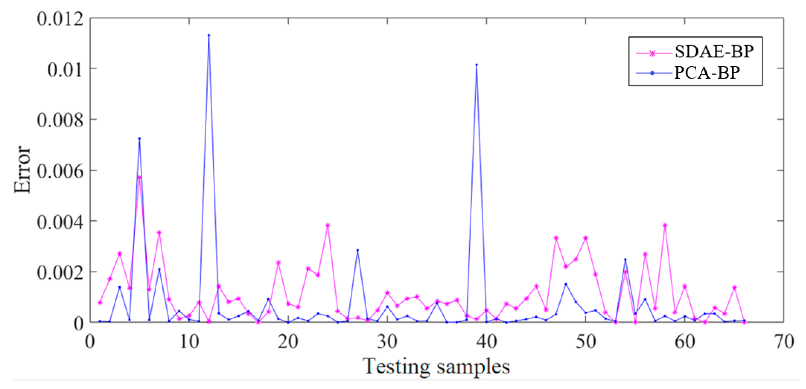
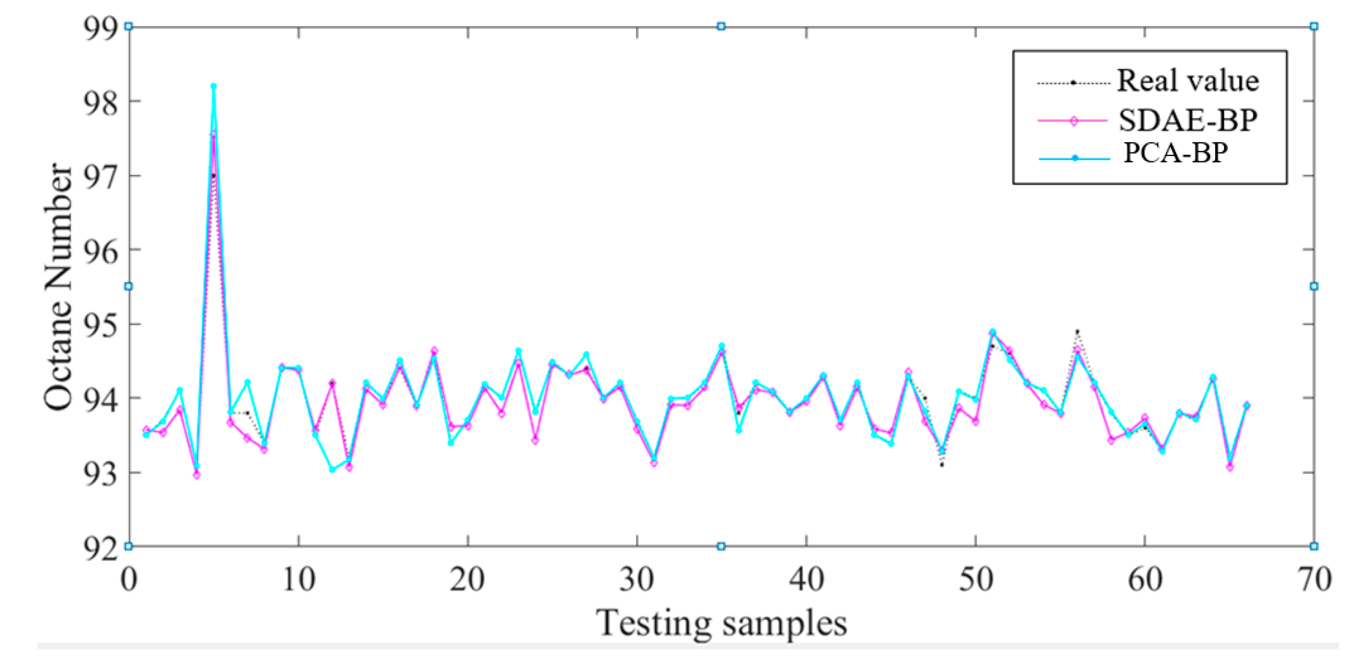
As shown in Figure 7, in the process of training, the training error of SDAE-BP is obviously lower than the PCA-BP. The Figure 8 reveals that the test error of SDAE-BP is also lower than PCA-BP. Additionally, Figure 9 shows the line charts of the predicted value of the predicted value and the real octane number of the two methods and the real octane number, the SDAE-BP is closer to the real one. Table 2 compares SDAE-BP and PCA-BP in several details, and shows that SDAE-BP is superior both in speed and accuracy. The results also mean that applying the model to octane online prediction is more effective.
The four groups of regression curves with different predictions are shown in Figure 10, in the training and validation process, the regression performance is significant (R at 0.99168 in training and R at 0.96943 in validation), which may cause overfitting. However, the test result dispels our doubt, the model generalization ability is very strong (the R is as high as 0.9734). The lines of fit are almost consistent with the target lines of fit, and the average R value is as high as 0.98556, which means that the prediction results are accurate and robust.
To sum up, from the perspective of training error, test error, R2, and other details, the robustness and performance of octane number soft sensor is greatly improved by using the SDAE-BP method.
5. Conclusions
To realize the prediction of octane number in the gasoline blending process, considering the efficiency of deep learning for parameter expression, a novel deep learning based soft sensor strategy by using the NIR spectroscopy obtained in the gasoline blending process is proposed. In this method, the stacked denosing auto-encoder (SDAE) is trained based on unlabeled NIR. In the training process, the gradient descent strategy is applied to update parameter and L2 regularization tragic, which can avoid overfitting, is used to optimize the loss function. Then, BP is initialized by trained SDAE, which can avoid to local minimums and accelerate convergence. For online dynamic data, SDAE-BP achieves fast and accurate prediction. In the future, SDAE may realize dimension reduction in the complex industry process to accurately predict results.
Author Contributions
Y.T., X.Y. and X.H. conceived, designed and performed the experiments and wrote the paper.
Funding
This research was funded by the Shanghai Sailing Program, grant number: 17YF1428300, and the Shanghai University Youth Teacher Training Program, grant number: ZZslg16009.
Acknowledgments
The authors would like to thank the anonymous reviewers for their valuable suggestions and comments.
Conflicts of Interest
The authors declare no conflict of interest. The founding sponsors had no role in the design of the study; in the collection, analyses, or interpretation of data; in the writing of the manuscript, and in the decision to publish the results.
References
- Balabin, R.M.; Safieva, R.Z.; Lomakina, E.I. Near-infrared (NIR) spectroscopy for motor oil classification: From discriminant analysis to support vector machines. Microchem. J. 2011, 98, 121–128. [Google Scholar] [CrossRef]
- He, K.; Cheng, H.; Du, W.; Qian, F. Online updating of NIR model and its industrial application via adaptive wavelength selection and local regression strategy. Chemom. Intell. Lab. Syst. 2014, 134, 79–88. [Google Scholar] [CrossRef]
- Cao, P.F.; Luo, X.L. Modeling of soft sensor for chemical process. CIESC J. 2013, 64, 788–800. [Google Scholar]
- Wang, X.; Liu, H. Soft sensor based on stacked auto-encoder deep neural network for air preheater rotor deformation prediction. Adv. Eng. Inform. 2018, 36, 112–119. [Google Scholar] [CrossRef]
- Li, C.; Ding, Z.; Qian, D.; Lv, Y. Data-driven design of the extended fuzzy neural network having linguistic outputs. J. Intell. Fuzzy Syst. 2018, 34, 349–360. [Google Scholar] [CrossRef]
- Andrade, J.M.; Prada, D.; Muniategui, S.; Lopez, P. Prediction of FCC gasoline octane numbers using FT-MIR and PLS. Anal. Bioanal. Chem. 1996, 355, 723. [Google Scholar] [CrossRef] [PubMed]
- Creton, B.; Dartiguelongue, C.; Bruin, T.D.; Toulhoat, H. Prediction of the Cetane Number of Diesel Compounds Using the Quantitative Structure Property Relationship. Energy Fuels 2010, 24, 5396–5403. [Google Scholar] [CrossRef]
- Yao, X.; Dai, L. A least squares SVM algorithm for NIR gasoline octane number prediction. In Proceedings of the WCICA 2004 Fifth World Congress on Intelligent Control and Automation, Hangzhou, China, 15–19 June 2004; Volume 4, pp. 3779–3782. [Google Scholar]
- Wang, T.; Dai, L.K.; Wan-Wu, M.A. Quantitative Analysis of Blended Gasoline Octane Number Using Raman Spectroscopy with Backward Interval Partial Least Squares Method. Chin. J. Anal. Chem. 2018, 46, 623–629. [Google Scholar]
- Gonzaga, J.C.; Meleiro, L.A.; Kiang, C.; Filho, R.M. ANN-based soft-sensor for real-time process monitoring and control of an industrial polymerization proces. Comput. Chem. Eng. 2009, 33, 43–49. [Google Scholar] [CrossRef]
- Rani, A.; Singh, V.; Gupta, J.R. Development of soft sensor for neural network based control of distillation column. ISA Trans. 2013, 52, 438–449. [Google Scholar] [CrossRef]
- Gao, J.; Yao, C.; Zhang, J. Application of Artificial Neural Network for the Prediction of Gasoline Octane Number by Near-infrared Spectroscopy. J. Anal. Sci. 2006, 22, 71–73. [Google Scholar] [CrossRef]
- Angelov, P.; Buswell, R. Identification of evolving fuzzy rule-based models. IEEE Trans. Fuzzy Syst. 2002, 10, 667–677. [Google Scholar] [CrossRef] [Green Version]
- Arazo, M.J.; Cano, J.M.; Gmez, S.E.; López, M.J.N.; Dimitriadis, Y.A.; López, J.Z. Automatization of a penicillin production process with soft sensors and an adaptive controller based on neuro fuzzy systems. Control Eng. Pract. 2004, 12, 1073–1090. [Google Scholar] [CrossRef]
- Wang, Y.H.; Huang, D.X.; Gao, D.J.; Jin, Y.H. Wavelet networks based soft sensor and predictive control in fermentation process. Comput. Aided Chem. Eng. 2003, 15, 1222–1227. [Google Scholar] [CrossRef]
- Jimenz, A.; Beltran, G.; Aguilera, M.P.; Uceda, M. A sensor-software based on artficial neural network for the optimization of olive oil elaboration process. Sens. Actuators B. Chem. 2008, 129, 985–990. [Google Scholar] [CrossRef]
- Lee, H.; Ekanadham, C.; Ng, A.Y. Sparse deep belief net model for visual areaV2. In Advances in Neural Information Processing Systems; The MIT Press: Cambridge, MA, USA, 2008; pp. 873–880. [Google Scholar]
- Vincent, P.; Larochelle, H.; Bengio, Y.; Manzagol, P.A. Extracting and composing robust features with denoising autoencoders. In Proceedings of the 25th International Conference on Machine Learning, Helsinki, Finland, 5–9 July 2008; pp. 1096–1103. [Google Scholar]
- Rifai, S.; Vincent, P.; Muller, X.; Glorot, X.; Bengio, Y. Contractive auto-encoders: Explicit invariance during feature extraction. In Proceedings of the 28th International Conference on Machine Learning (ICML-11), Bellevue, WA, USA, 28 June–2 July 2011; pp. 833–840. [Google Scholar]
- Hinton, G.E.; Srivastava, N.; Krizhevsky, A.; Sutskever, I.; Salakhutdinov, R.R. Improving neural networks by preventing co-adaptation of feature detectors. Comput. Sci. 2012, 3, 212–223. [Google Scholar]
- Qi, Y.; Shen, C.; Wang, D.; Shi, J.; Jiang, X.; Zhu, Z. Stacked Sparse Autoencoder-Based Deep Network for Fault Diagnosis of Rotating Machinery. IEEE Access 2017, 5, 15066–15079. [Google Scholar] [CrossRef]
- Menafoglio, A.; Grasso, M.; Secchi, P.; Colosimo, B.M. Profile Monitoring of Probability Density Functions via Simplicial Functional PCA with application to Image Data. Technometrics 2018, 19. [Google Scholar] [CrossRef]
- Guan, N.; Tao, D.; Luo, Z.; Yuan, B. Manifold Regularized Discriminative Nonnegative Matrix Factorization with Fast Gradient Descent. IEEE Trans. Image Process. 2011, 20, 2030–2048. [Google Scholar] [CrossRef]
- An, S.Y.; Kang, J.G.; Choi, W.S.; Oh, S.Y. A neural network based retrainable framework for robust object recognition with application to mobile robotics. Appl. Intell. 2011, 35, 190–210. [Google Scholar] [CrossRef]
- Amihud, Y.; Goyenko, R. Mutual Fund’s R2 as Predictor of Performance. Rev. Financ. Stud. 2013, 26, 667–694. [Google Scholar] [CrossRef]
- Rubinstein, R.Y.; Kroese, D.P. The Cross-Entropy Method. Technometrics 2008, 50, 92. [Google Scholar] [CrossRef]
- Bengio, Y. Practical Recommendations for Gradient-Based Training of Deep Architectures. In Neural Networks: Tricks of the Trade; Springer: Berlin/Heidelberg, Germany, 2012; pp. 437–478. [Google Scholar]
- Nebauer, C. Evaluation of convolutional neural networks for visual recognition. IEEE Trans. Neural Netw. 1998, 9, 685–696. [Google Scholar] [CrossRef] [PubMed]
Figure 1.
Spectral wavelength diagram.

Figure 2.
The neural network structure of the auto- encoder (AE).

Figure 3.
Schematic diagram of denosing auto-encoder (DAE).

Figure 4.
Schematic diagram of stacked denosing auto-encoder (SDAE).

Figure 5.
Schematic diagram of gradient descend.

Figure 6.
Schematic diagram of SDAE-BP Model.

Figure 7.
Schematic diagram of SDAE-BP Model.

Figure 8.
The testing error curves of SDAE-BP and PCA-BP.

Figure 9.
The prediction curves of SDAE-BP and PCA-BP.

Figure 10.
Schematic diagram of SDAE-BP Model.


Table 1.
The comparison diagram of soft sensor models.
| Model Type | Time (s) | R2 | MSE |
|---|---|---|---|
| PCA-BP | 20.1 | 0.86358 | 0.04271 |
| SDAE-BP(1 layers) 9 | 17.9 | 0.92576 | 0.02335 |
| SDAE-BP(2 layers) 9-9 | 21.5 | 0.92941 | 0.02284 |
| SDAE-BP(3 layers) 9-9-9 | 19.8 | 0.89140 | 0.035684 |
| SDAE-BP(4 layers) 9-9-9-9 | 16.9 | 0.94752 | 0.02334 |
| SDAE-BP(5 layers) 9-9-9-9-9 | 24.2 | 0.72975 | 0.08730 |
Table 2.
The comparison diagram of soft sensor models.
| Details | PCA-BP | SDAE-BP |
|---|---|---|
| Training error | 0.02189 | 0.00892 |
| Testing error | 0.00823 | 0.00391 |
| Training time (s) | 20.1 | 16.9 |
| R2 of prediction | 0.86358 | 0.94752 |
| MSE of prediction | 0.04271 | 0.02334 |
© 2018 by the authors. Licensee MDPI, Basel, Switzerland. This article is an open access article distributed under the terms and conditions of the Creative Commons Attribution (CC BY) license (http://creativecommons.org/licenses/by/4.0/).
Share and Cite
MDPI and ACS Style
Tian, Y.; You, X.; Huang, X. SDAE-BP Based Octane Number Soft Sensor Using Near-infrared Spectroscopy in Gasoline Blending Process. Symmetry 2018, 10, 770. https://0-doi-org.brum.beds.ac.uk/10.3390/sym10120770
AMA Style
Tian Y, You X, Huang X. SDAE-BP Based Octane Number Soft Sensor Using Near-infrared Spectroscopy in Gasoline Blending Process. Symmetry. 2018; 10(12):770. https://0-doi-org.brum.beds.ac.uk/10.3390/sym10120770
Chicago/Turabian StyleTian, Ying, Xinyu You, and Xiuhui Huang. 2018. "SDAE-BP Based Octane Number Soft Sensor Using Near-infrared Spectroscopy in Gasoline Blending Process" Symmetry 10, no. 12: 770. https://0-doi-org.brum.beds.ac.uk/10.3390/sym10120770
Note that from the first issue of 2016, this journal uses article numbers instead of page numbers. See further details here.