Connecting Electroweak Symmetry Breaking and Flavor: A Light Dilaton D and a Sequential Heavy Quark Doublet Q

Abstract

The 125 GeV boson is quite consistent with the Higgs boson of the Standard Model (SM), but there is a challenge from Anderson as to whether this particle is in the Lagrangian. As Large Hadron Collider (LHC) Run 2 enters its final year of running, we ought to reflect and make sure we have gotten everything right. The ATLAS and CMS combined Run 1 analysis claimed a measurement of 5.4$\sigma$ vector boson fusion (VBF) production which is consistent with SM, which seemingly refutes Anderson. However, to verify the source of electroweak symmetry breaking (EWSB), we caution that VBF measurement is too important for us to be imprudent in any way, and gluon–gluon fusion (ggF) with similar tag jets must be simultaneous measured, which should be achievable in LHC Run 2. The point is to truly test the dilaton possibility—the pseudo-Goldstone boson of scale invariance violation. We illustrate EWSB by dynamical mass generation of a sequential quark doublet (Q) via its ultrastrong Yukawa coupling and argue how this might be consistent with a 125 GeV dilaton, $\mathcal{D}$. The ultraheavy $2m_Q\gtrsim 4$–5 TeV scale explains the absence of New Physics so far, while the mass generation mechanism shields us from the UV theory for the strong Yukawa coupling. Collider and flavor physics implications are briefly touched upon. Current Run 2 analyses show correlations between the ggF and VBF measurements, but the newly observed $t\overline{t}H$ production at LHC poses a challenge.

1. Higgs, Anderson, and All That

Spontaneous symmetry breaking (SSB) was introduced into particle physics by Nambu as cross-fertilization from superconductivity (SC). In an explicit model with Jona-Lasinio (NJL), Nambu illustrated [1] how the nucleon mass $m_N$ could arise from dynamical chiral symmetry breaking (D$\chi$SB), with the pion emerging as a pseudo-Nambu–Goldstone (NG) boson. Subsequent work lead to the Brout-Englert-Higgs (BEH) mechanism [2,3] of electroweak symmetry breaking (EWSB), which became [4,5] part of the Standard Model (SM). The recently discovered 125 GeV boson [6,7] seems consistent with the Higgs boson of SM on every count. This has, in turn, stimulated condensed matter physicists to pursue their own “Higgs” mode.

A “Higgs” mode was recently observed [8] in disordered SC films near the SC-insulator quantum critical point, far below the $2\Delta$ double-gap threshold. Here, $\Delta$ is the “energy gap” of the SC phase which is maintained throughout the experiment. This “light Higgs” mode contrasts with “amplitude modes” around $2\Delta$ that were claimed long ago [9]. Anderson, who originated the nonrelativistic version of the BEH mechanism, praised [10] Nambu for elucidating [1] the dynamical generation of $m_N$, a “mass gap”, by drawing analogy with SC: a scalar boson in NJL-type of models with mass $\sim 2$$m_N$ is an “amplitude mode”. Anderson then turned to challenge particle physics [10]: “If superconductivity does not require an explicit Higgs in the Hamiltonian to observe a Higgs mode, might the same be true for the 126 GeV mode?", hence jesting “Maybe the Higgs boson is fictitious!" He then stressed the importance of Ref. [8], as “it bears on the nature of the Lagrangian of the Standard Model”.

As Anderson coined the word “emergent” [11] for phenomena that are not inherent in the Lagrangian, he challenges the elementary nature of 125 GeV boson.

What do we really know about 125 GeV boson? If it is not the Higgs boson (H) of SM, then what else could it be? In this paper, we revamp the idea that the observed boson could still be a dilaton ($\mathcal{D}$) from spontaneous scale invariance violation. We argue that this can be truly excluded only by data-based simultaneous measurement of both the vector boson fusion (VBF) process and gluon–gluon fusion (ggF) plus similar tag jets. This will hopefully be achievable with Run 2 data at the Large Hadron Collider (LHC), despite the existing claim [12] with Run 1 data. We then elucidate how EWSB might arise from dynamical mass generation of a sequential quark doublet (Q) through its ultrastrong Yukawa coupling, resulting in $2m_Q$ that is far above 125 GeV, which echoes the result of Ref. [8]. One should, of course, avoid directly matching a dilaton with the “Higgs” mode of Ref. [8].

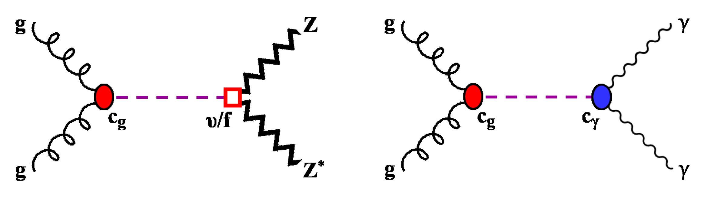
The discovery of 125 GeV boson is perceived as being due to ggF production and driven by $Z{Z}^{\ast }$ (two lepton pairs) and $\gamma \gamma$ channels, as illustrated in Figure 1. It is usual to measure the relative strength with respect to (w.r.t.) SM, ${\mu \equiv (\sigma ·\mathcal{B})/(\sigma ·\mathcal{B})|}_{\mathrm{SM}}$ (i.e., 1 for H of SM). In terms of the coefficients $c_g$, $\widehat{v}\equiv v/f\equiv 1/\widehat{f}$ (meaning of f defined later) and $c_{\gamma }$, as illustrated in Figure 1, of the $gg$, $ZZ$ and $\gamma \gamma$ couplings of the 125 GeV boson w.r.t. SM, what ATLAS + CMS observe [12] is

$${\mu }_{Z{Z}^{\ast }}\cong \frac{c_g^2{\widehat{v}}^2}{0.910{\widehat{v}}^2+0.0868c_g^2}\simeq 1,$$

(1)

$${\mu }_{\gamma \gamma }\cong \frac{c_g^2{c}_{\gamma }^2}{0.910{\widehat{v}}^2+0.0868c_g^2}\gtrsim 1,$$

(2)

where we assume $v/f$ applies also to fermions, that the tiny $\gamma \gamma$ and $Z\gamma$ decays in the denominator are ignored, and that the the invisible width ${\mathsf{\Gamma }}_{\mathrm{inv}}$ is absent. We took nominal values of SM decay rates for the final states of $V{V}^{\ast }$ and $f\overline{f}$, and used ${\mathsf{\Gamma }}_{\mathrm{SM}}\simeq 4$ MeV. Thus, the denominator in above equations is nothing but $\mathsf{\Gamma }/{\mathsf{\Gamma }}_{\mathrm{SM}}$.

Equation (1) is, of course, satisfied by the SM case of $c_g$, $\widehat{v}\simeq 1$. However, if one allows $c_g>1$, then the allowed value for $1/\widehat{v}$ increases, which onsets quickly (hence, the width of $\mathsf{\Gamma }$ drops first as $c_g$ increases from 1, before picking up for large $c_g$), but saturates to $f/v\simeq 1/\sqrt{0.0868}\simeq 3.394$ as $c_g\to \infty$, which can be seen easily from Equation (1). For example, $f/v\simeq 2$, 3, 3.22, 3.33, respectively, for $c_g\simeq 1.18$, 2.04, 3.0, 4.93. The mild inequality of Equation (2) is easier to satisfy. Besides $c_g,\widehat{v}\simeq 1$, for the aforementioned values of $(c_g,\widehat{f})\simeq (1.18,2)$, (2.04, 3), (3.0, 3.22), (4.93, 3.33), one has $|c_{\gamma }|\gtrsim 0.50$, 0.333, 0.311, 0.30, respectively, reaching the asymptotic $\sqrt{0.0868}\simeq 0.295$ for very large $c_g$. These examples for $c_g$, $v/f$ and $|c_{\gamma }|$ came as a result of Higgs width and branching ratio considerations.

For large $c_g$ and with $V{V}^{\ast }$ and $f\overline{f}$ rates suppressed by $v/f$, the predominant decay will be the $gg$ mode, just as in production. New Physics could affect the allowed $c_g$, $v/f$ and $c_{\gamma }$ values, but just the presence of ${\mathsf{\Gamma }}_{\mathrm{inv}}$ would only make matters worse, as it would disallow a compensating effect of smaller $\widehat{v}$.

Measurements are remarkably consistent with SM, but one should probe individual coefficients directly. If the 125 GeV boson is a dilaton ($\mathcal{D}$), the (pseudo-)NG boson from SSB of scale invariance, then $c_g$ and $c_{\gamma }$ are determined by the trace anomaly of the energy momentum tensor, which would depend on the beta functions of QCD and QED, respectively, while $v/f$ is a common factor that was mentioned by Altarelli [13] as late as 2013: “The Higgs couplings are proportional to masses: a striking signature ...”, but “also true for a dilaton, up to a common factor”. Thus, f is the dilaton decay constant.

That a dilaton could be confused for a light SM Higgs boson was stressed by Ref. [14] in 2008, before the advent of LHC. However, the example given was to have QCD and QED “embedded in the conformal sector at high scale”; hence, $c_{\gamma }=-17/9$, and $c_g=11-2N_{\mathrm{light}}/3=23/3$, a case (and similar large values) that is definitely ruled out [15], causing many to write-off the dilaton. In fact, early papers [16,17,18] on dilaton interpretation of the new 125 GeV boson noted that data preferred “Higgs-like” dilaton of $f\simeq v$, which is not what we advocate. For example, starting from the $c_g$, $c_{\gamma }$ and $v/f$ parametrization, Ref. [18] showed that $v/f\sim 1/3$ was already ruled out by early Run 1 data. On closer inspection, however, the authors of Ref. [18] themselves scaled $c_g$, $c_{\gamma }$ by $v/f$, which is opposite to the trend of large values from Ref. [14], and we are not certain of the full generality of these results. In view of the Anderson challenge, dilaton should be kept in mind and tested without prejudice with the purist criteria of Elander and Piai [19] of keeping $c_g$, $v/f$ and $c_{\gamma }$ as parameters.

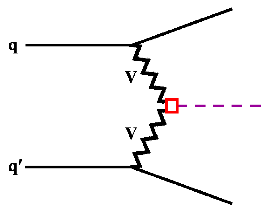
One might say that the $VV$ coupling has already been measured with Run 1 data—the combined analyses of the ATLAS and CMS experiments together claimed a $5.4\sigma$ measurement of VBF production [12], finding consistency with SM; hence, $v/f\sim 1$, which would run against the possibility of dilaton. It is certainly true, and very important, that the $VV$ coupling of the 125 GeV boson can be probed directly by the VBF process, as illustrated in Figure 2. In the following section, we begin with a critique of this 5.4$\sigma$ measurement, cautioning that it may still be premature. We update with Run 2 results that have become available, but defer it to Section 5.

In this paper, we take the experimentally observed 125 GeV boson as the dilaton ($\mathcal{D}$), without accounting for its true origins. We revamp the case for dynamical EWSB by ultrastrong Yukawa coupling of a sequential quark doublet (Q), and elucidate why it might be consistent with the emergence of a dilaton. The approach shields one from the high energy completion behind this strong Yukawa coupling, including the origin of scale invariance breaking, hence the emergence of the dilaton itself.

2. On Observing VBF

We first note that the Run 1 VBF measurements by ATLAS and CMS are not individually significant yet, as the cross section of the leading ggF process in SM is ∼1/12. Combining datasets when analyses are still limited by statistics is suitably common. However, the combined analysis of LHC Run 1 data by ATLAS and CMS which claimed the 5.4$\sigma$ measurement of the VBF process has some weaknesses. We offer here some simple critique, with discussion of Run 2’s situation deferred to Section 5.

First, we present an issue of semantics. Recall the usage of Higgs-like for 125 GeV boson up to early 2013. By the same token, in Run 1, one is really probing VBF-like production, rather than genuine VBF. This is because it is based on a multivariate analysis of categorized data [12]. As the radiation of vector boson (V) is rather analogous to synchrotron radiation, it is effective only when each “spent” quark retains most of the initial parton momentum. But since $m_V$ is sizable, genuine VBF requires two ultra-energetic tag jets that are necessarily back-to-back [20] with large $m_{j_1{j}_2}$ and large rapidity separation, and little color radiation in the rapidity gap. The categorized analysis is a compromise due to limited statistics. If statistics were sufficient, one should always cross-check with a high purity VBF selection (cut-based analysis) that beats the ggF background down to a true minimum.

Second, with ggF production being the leading process, one needs to explore analysis methods to simultaneously measure both VBF and ggF production with similar tag jets, methods that require statistical power to achieve the separation. The current VBF measurement relies on predicting the jet-tagged ggF yield in the two-jet (VBF-like) category, ggF+jj, and subtracting it from the measured yield [21]. Although this extrapolation relies on Monte Carlo, experimentally, the MC predictions for the 0-, 1- and 2-jet categories are checked with data, and the systematic uncertainty of extrapolation, though not small, is under control. As integrated luminosity accumulates, the separation power between VBF and ggF+jj will improve and eventually lead to a systematic error on VBF that is lower than the one provided by the current subtraction method. In this case, biases coming from the ggF side are removed, and systematics are due to the level of control of ggF and VBF kinematic distributions.

Third, the prominence of the “Higgs boson” discovery means that bias necessarily seeps into the analyses, especially after the 2013 Nobel prize. However, there is no good way to combine potential biases [22]. Finally, the $5\sigma$ claim has the connotation that observation has been achieved. However, identifying the true source of EWSB is too important an issue to not keep the highest standards.

We advocate that one should await the verdict on VBF from the much larger dataset of LHC Run 2 which is already two-thirds its way through. Note that, despite some hints of $t\overline{t}H$ production in both Run 1 [12] and early 13 TeV data [23], they are less significant. We turn to a brief survey of currently available Run 2 results in Section 5.

In view of Anderson’s challenge, we take 125 GeV boson as an emergent dilaton, and turn to recount how a new sequential quark doublet (Q) could self-generate $m_Q$ through its ultrastrong Yukawa coupling. This dynamical EWSB mechanism may allow a dilaton to emerge, but does not quite explain it.

The fourth generation (4G) model was supposedly “killed by the Higgs discovery” [24], because adding $t^{\prime }$, $b^{\prime }$ to t in the triangle loop for $ggH$ coupling would enhance the amplitude by ∼3; hence, the cross section would be enhanced by 9, which is not observed [6,7]. However, there is nothing really wrong with 4G quarks, except this “Higgs” cross section which could be due to a dilaton, as we have just stressed. As already commented, $c_g\gtrsim 3$, compensated by $v/f\sim$ 1/3 with appropriate $c_{\gamma }$ also gives ${\mu }_{Z{Z}^{\ast }}\sim 1$ and ${\mu }_{\gamma \gamma }\gtrsim 1$.

3. The Yukawa Coupling Enigma

Yukawa couplings of fermions are an enigma, but an elementary Higgs field is not needed to define them. There is a dynamical difference between the electroweak (EW) theory and QED and QCD, where decoupling [25] is the rule. Nondecoupling of heavy quarks in EW processes, such as EW penguin effects in $b\to s{\ell }^{+}{\ell }^{-}$ [26], is rooted in the Yukawa coupling, which grows with mass.

As this author was learning particle physics, SM began to enter textbooks, so the Lagrangian was taken for granted. The SM Lagrangian has a built-in complex scalar doublet, and it was Weinberg who introduced [4] the Yukawa coupling for fermion mass generation.

By time of LHC turn-on, however, the weak vertex

$$\frac{1}{\sqrt{2}}g{V}_{ij}{\overline{u}}_i{\gamma }_{\mu }L{d}_j{W}^{\mu },$$

(3)

had become firmly established with LEP and B factory data. Since all particles in Equation (3) are massive, and since the longitudinal $W_L$ propagates with the $\frac{k_{\mu }{k}_{\nu }}{M_W^2}$ factor, replacing $W^{\mu }$ by $\frac{k_{\mu }}{M_W}$ in Equation (3) and using the Dirac equation, one gets [27]

$$\frac{1}{\sqrt{2}}{V}_{ij}{\overline{u}}_i\left({\lambda }_{i}L-{\lambda }_{j}R\right)d_{j}G.$$

(4)

The weak coupling g cancels against $M_W=\frac{1}{2}gv$, and

$$\frac{{\lambda }_Q}{\sqrt{2}}\equiv \frac{m_Q}{v},$$

(5)

is exactly the Yukawa coupling of the NG boson (G), with both left- and right- chiral couplings emerging from a purely left-handed vector coupling! The point is that no Lagrangian is used; hence, Yukawa couplings are experimentally established, and the longitudinal $W_L$ is the “eaten” NG boson, without touching upon whether there is an elementary Higgs boson or field.

One may say that the above is nothing but the Goldstone theorem [28,29]. What we have elucidated is that all of our knowledge of Yukawa couplings, including the Cabibbo-Kobayashi-Maskawa (CKM) matrix elements $V_{ij}$ and the unitarity of V, are extracted through their dynamical, nondecoupling effects. They arise from the NG bosons without reference to an elementary Higgs doublet field or its remnant particle.

Anderson’s point, then, is that we need to make sure the 125 GeV boson is, in fact, the remnant of a complex scalar doublet in the SM Lagrangian, as we have discussed in the previous section.

However, Yukawa couplings are truly an enigma—we know not what determines their values that range from ${\lambda }_{u,d}\sim {10}^{-5}$ to ${\lambda }_t\cong 1$, are modulated by $V_{ij}$ and exhibit a hierarchical pattern. They are the sources of all known flavor physics and $CP$ violation (CPV). With quark Yukawa couplings spanning five orders already, we now argue that raising by another order to the “extremum” value of ${\lambda }_Q\gtrsim 4\pi$ could induce dynamical EWSB.

4. Ultrastrong Yukawa-Induced EWSB and the Dilaton

After the restart of LHC by 2010 search limits on $m_{b^{\prime }}$, $m_{t^{\prime }}$ rose quickly beyond the nominal “unitarity bound” [30,31] of ∼550 GeV, but the search continued for unitarity bound violating (UBV) 4G quarks. The heavy mass just implies very strong Yukawa coupling, and the EW precision observables, S and T, demand nearly degenerate [32,33] $t^{\prime }-b^{\prime }$; hence, we denote the doublet as Q. Note that a small $m_{t^{\prime }}-m_{b^{\prime }}$ splitting is needed to compensate [32] for S and T as $m_Q$ and the Higgs mass both become very heavy.

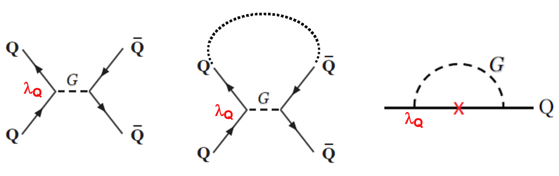
UBV implies bad high energy (H.E.) behavior for $Q\overline{Q}\to Q\overline{Q}$ scattering, which is dominated by G (i.e., $V_L$) exchange, as shown in Figure 3 (left). The range of interaction, $1/M_W$, becomes large compared with $1/m_Q$ for heavier Q values. This runs against intuition for short distance or UV remedy of the bad H.E. behavior, whether based on UBV or NJL folklore. By linking [27] a Q to a $\overline{Q}$ across the exchanged G, as shown in Figure 3 (center), the $Q\overline{Q}\to Q\overline{Q}$ scattering turns into the self-energy of Q, where the exchange momentum (q) is summed over. This becomes a “gap equation” for the generation of $m_Q$, the “mass gap”, as illustrated in Figure 3 (right), with the cross (×) representing the self-energy function itself. A nontrivial solution would mean mass generation. As the chiral symmetry is the SU(2)${}_{\mathrm{L}}$ gauge symmetry, D$\chi$SB means dynamical EWSB, which the reverse of Weinberg [4].

The self-energy in Figure 3 (right) differs from NJL [1], which uses a dimension-6 four-quark operator that leads to a closed “bubble” with a freely running loop momentum (q) but is independent of external momentum (p), with the cutoff ($\mathsf{\Lambda }$) provided by the operator coefficient. In contrast, the NG boson loop of Figure 3(right) manifests the long-distance nature, while the $QQG$ coupling brings the external momentum (p) into the loop. Thus, the Yukawa-induced gap equation is different from NJL and more intricate. Note that there is no scale parameter: $m_Q^0=0$ at tree level by gauge invariance.

To formulate the gap equation for the mathematical solution, one needs to fix the range of integration for q. With no New Physics found from 1 to several TeV by summer 2011, the self-consistent and simplest ansatz [27] is to integrate $q^2$ up to ${\left(2m_Q\right)}^2$, such that the NG boson G in the loop is justified. By keeping ${\lambda }_Q$, defined in Equation (5) as a parameter, the scale (v) is brought in to make contact with the experiment.

With this ansatz of integration limit being twice the generated mass ($m_Q$), the gap equation was solved numerically [34] in the ladder approximation. Despite the urge to keep $m_Q$ below TeV for the sake of LHC phenomenology, a nontrivial solution demanded

$${\lambda }_Q\gtrsim 4\pi ,(m_Q\gtrsim 2\mathrm{TeV}!),$$

(6)

i.e., at “Naive Dimensional Analysis” (NDA) strong coupling [35] of $4\pi$ or higher [36], D$\chi$SB, and hence, dynamical EWSB, can occur at “extremum” coupling strength! Shortly after submission, however, 125 GeV boson was announced [6,7], so it took one and half years to get the work published [34], which was largely ignored.

The challenge from Anderson [10], however, throws a different light. In the Yukawa-dynamical EWSB, the self-energy sums over $Q\overline{Q}\to Q\overline{Q}$ scattering; hence, it is a pairing mechanism, much like the Cooper pairs of the Bardeen-Cooper-Schriefer (BCS) theory of superconductivity which NJL tried to emulate [1]. We have already expounded the difference with NJL, and the numerical solution suggested that EWSB occurs at an NDA-strong strength of $4\pi$; hence, perturbation has broken down absolutely [35]. For ${\lambda }_Q$, consistent with Equation (6), $m_Q$ is generated, which means a $Q\overline{Q}$ condensate has formed; hence, the exactly massless NG boson G is, in fact, a $Q\overline{Q}$ boundstate. All these can be viewed from the perspective of $Q\overline{Q}$ scattering in the massive world [37]. This dynamical mechanism can induce EWSB without ever having an “explicit” Higgs in the Lagrangian. Additionally, much like the NJL model, there should be “amplitude” modes, such as scalar bosons, around $2m_Q\sim 4$–5 TeV.

We did not [34], however, anticipate a light boson far below $2m_Q$, but a light 125 GeV boson emerged. In face of the challenge by Anderson, we take this to be a dilaton [38]. However, how does this make sense in context?

Recall that our gap equation based on Yukawa coupling (${\lambda }_Q$) has no scale, and contact with v was introduced self-consistently by ansatz of integration up to $2m_Q=\sqrt{2}{\lambda }_{Q}v$. There was a nontrivial numerical solution to our no-scale formulation; hence, $m_Q$ generation would also seemingly break scale invariance. This may allow a dilaton ($\mathcal{D}$) to emerge [39], but we neither predicted this, nor do we know how $m_{\mathcal{D}}$ is generated. The dilaton should arise from the true origin of scale invariance violation which we conjecture to be the theory of strong Yukawa coupling that explains Equations (5) and (6). As elucidated in Section 3, Yukawa couplings arise empirically from EW physics without the need for a Higgs field to define them. Note that $Q\overline{Q}$ condensation and the integration limit of $2m_Q$ shield us from the actual UV theory, which is likely not far beyond the rather high $2m_Q$ (because of the strong ${\lambda }_Q$). We do not know what this is, except that it is strongly coupled and likely conformal [14,16,17,18].

So, we have New Physics both within and beyond SM. Rather than the Higgs field, the agent of mass, or EWSB, is $Q\overline{Q}$ condensation via its own ultrastrong ${\lambda }_Q$. The 125 GeV boson is a dilaton ($\mathcal{D}$) that descends from some unknown UV sector; unlike the NG boson G, it cannot be a pure $Q\overline{Q}$ boundstate.

5. LHC Run 2 Results

The original version of this essay was prepared around the time of the ATLAS and CMS Run 1 combined analaysis [12]. Since then, some Run 2 results (13 TeV) have become available, and it is necessary to check how our discussion so far survives data scrutiny. We see that our scenario remains potent, and, in fact, ggF vs VBF production measurements do show some “symptoms”. However, the observation by both ATLAS and CMS, of $t\overline{t}H$ production poses a challenge.

Without quoting detailed errors and often dropping insignificant results without comment, let us give a brief survey of what is currently available:

• ${\mathit{ZZ}}^{\ast }$: Both experiments have made the analyses up to 2017 data available at 79.8 fb${}^{-1}$ and 77.4 fb${}^{-1}$, respectively, for ATLAS and CMS.
  For ATLAS [40], while ${\mu }_{\mathrm{ggF}}\simeq 1$ is measured, the ${\mu }_{\mathrm{VBF}}\simeq 2.8$ value is rather large.
  For CMS [41], ${\mu }_{\mathrm{ggF},\mathrm{b}\overline{\mathrm{b}}\mathrm{H}}={1.15}_{-0.16}^{+0.18}$ is measured and ${\mu }_{\mathrm{VBF}}={0.69}_{-0.57}^{+0.75}$ is barely 1$\sigma$, reflecting, in part, the absence of events in the 2016 data (36.9 fb${}^{-1}$).
  Could these “fluctuations” reflect a much larger ggF production rate but with an analysis strategy centered around SM expectation?
• $\mathit{\gamma }\mathit{\gamma }$: The results are for 36.1 fb${}^{-1}$ and 35.9 fb${}^{-1}$, respectively, (i.e., 2016 data) for ATLAS and CMS.
  For ATLAS [42], ${\mu }_{\mathrm{ggF}}={0.81}_{-0.18}^{+0.19}$ is mildly less than 1, but ${\mu }_{\mathrm{VBF}}={2.0}_{-0.5}^{+0.6}$ is, again, rather large.
  For CMS [43], ${\mu }_{\mathrm{ggF}}={1.10}_{-0.18}^{+0.20}$ looks reasonable, but ${\mu }_{\mathrm{VBF}}={0.8}_{-0.5}^{+0.6}$ is not inconsistent with zero.
  The trends for ATLAS and CMS are again opposite. In addition to the possibility that ggF production could be much stronger than assumed, this may reflect differences in analysis choice(s).
• ${\mathit{WW}}^{\ast }$: Both experiments are only for 2016 data.
  For ATLAS [44], the measured ${\sigma ·\mathcal{B}|}_{\mathrm{ggF}}$ at 6.3$\sigma$ is ≃$20\%$ larger than the SM expectation, while ${\sigma ·\mathcal{B}|}_{\mathrm{VBF}}$ is found at 1.9$\sigma$, w.r.t. SM expectation at 2.7$\sigma$.
  For CMS [45], ${\mu }_{\mathrm{ggF}}={1.38}_{-0.24}^{+0.21}$ is 1.6$\sigma$ above SM, while $\mathrm{VBF}={0.29}_{-0.29}^{+0.66}$ is consistent with zero, reflecting, in part, the null result in 2016 data.
• $\mathit{\tau }\mathit{\tau }$: Based on 2016 data, ATLAS has recently joined CMS in claiming observation. Given the large backgrounds for $gg\to H\to {\tau }^{+}{\tau }^{-}$, the observation was made with “jet assistance”.
  For CMS [46], $\mu ={1.09}_{-0.26}^{+0.27}$ is at 4.9$\sigma$ (combining with Run 1 to become 5.9$\sigma$) which combines the 0-jet, Boosted, and VBF measurements. Not surprisingly, 0-jet is barely 1$\sigma$, so the measurement comes from the latter two. However, our question of jet-tagged ggF vs. VBF remains.
  For ATLAS [47], combining Boosted and VBF categories gives 4.4$\sigma$ (4.1$\sigma$), improving to 6.4$\sigma$ (5.4$\sigma$) when combined further with Run 1. The expected SM significance is given in parenthesis.
• $\mathit{b}\overline{\mathit{b}}$: Both ATLAS and CMS find evidence for this. The large $b\overline{b}$ cross section from QCD implies jet-tag-assistance would not work, and measurements are based on $VH$ associated production, where both experiments use $VZ$ production for validation. By combining the 2016 data with Run 1, ATLAS [48] and CMS [49] experiments find evidence at 3.6$\sigma$ (4.0$\sigma$) and 3.8$\sigma$ (3.8$\sigma$), respectively. Both experiments find excess events in $m_{b\overline{b}}$ above the Z pole.
• Combinations: CMS has put out a combination of analyses based on 2016 data, while ATLAS has combination of only $Z{Z}^{\ast }$ and $\gamma \gamma$ modes.
  For CMS [50], ${\mu }_{\mathrm{ggF}}\simeq 1.23$ is about 1$\sigma$ above SM, while ${\mu }_{\mathrm{VBF}}\simeq 0.73$ is about 1$\sigma$ below. $WH$ is found to be large, about twice the SM expectation, while $ZH$ is consistent with SM and 2$\sigma$ away from zero.
  For ATLAS [51], ${\mu }_{\mathrm{ggF}}$ is consistent with 1, but ${\mu }_{\mathrm{VBF}}$ is greater than 2 and is rather large. $VH$ is found to be consistent with zero.
• $\mathit{t}\overline{\mathit{t}}\mathit{H}$: By adding the 2017 data for the $H\to Z{Z}^{\ast }$ and $\gamma \gamma$ modes, ATLAS has recently joined CMS in observation of $t\overline{t}H$ production at the LHC.
  For CMS [52], based on H decay to the five modes of $W{W}^{\ast }$, $Z{Z}^{\ast }$, $\gamma \gamma$, ${\tau }^{+}{\tau }^{-}$ and $b\overline{b}$, and combining 2016 data with Run 1, the measurement of ${\mu }_{t\overline{t}H}={1.26}_{-0.26}^{+0.31}$ makes a 5.2$\sigma$ observation.
  ATLAS [53] was a bit unlucky with a similar data set. Adding data from 2017 to $H\to Z{Z}^{\ast }$ and $\gamma \gamma$ and combining this with 2016 data for the other three modes gives ${\mu }_{t\overline{t}H}={1.32}_{-0.26}^{+0.28}$, achieving an observation of 5.8$\sigma$ (4.9$\sigma$) with 13 TeV data alone. Combined with Run 1, the significance becomes 6.3$\sigma$ (5.1$\sigma$).

So, what to make of the available 13 TeV results? For the two Run 1 drivers, $Z{Z}^{\ast }$ and $\gamma \gamma$, there are some apparent correlations or fluctuations between the ATLAS and CMS results on ggF vs VBF. While CMS shows a mild deficit for VBF, ATLAS shows a rather large excess, so perhaps our criticism given in Section 2 may have some bearing. As already raised above, this could be due to a much larger ggF production rate, compounded by analysis strategies based on a SM mindset (e.g., the underlying ggF, Monte Carlo). Rather than genuine VBF with very energetic forward and backward jets, perhaps what is measured is ggF with VBF-like double tag-jets.

The observation of $H\to {\tau }^{+}{\tau }^{-}$ is of significance for direct evidence of H coupling to fermions. However, given the nature of jet-assistance, our criticism remains that one cannot be sure that it is not actually jet-tag-assisted ggF production that is measured. For $W{W}^{\ast }$, both experiments seem to have observed ggF production, but the indication for VBF is quite weak. Without a mass bump, the analysis is quite different from $Z{Z}^{\ast }$ and $\gamma \gamma$, so our point of simultaneous measurement of ggF with VBF-like jet-tags and genuine VBF remains valid.

What may be a little worrisome is the evidence from both ATLAS and CMS for $b\overline{b}$ in $VH$ production. The production is quite distinct from ggF and should be suppressed if $v/f$ is of the order 1/3 or so, but there is clear excess in $m_{b\overline{b}}$ above $M_Z$ that we cannot explain.

The observation of $t\overline{t}H$ production with mild excess above SM for both ATLAS and CMS could be devastating to our proposed scenario. The process is nothing but H radiating off the QCD production of a $t\overline{t}$ pair; hence, direct measurement of $ttH$ coupling and consistency with SM expectation offers genuine support for the top Yukawa coupling, ${\lambda }_t\cong 1$. The process ought to be suppressed by the universal factor $v^2/f^2$ for the dilaton case. Even if a greatly enhanced $c_g$ leads to 125 GeV boson emission off a gluon line for the QCD production of $t\overline{t}$ pair, that it also mimics $t\overline{t}H$ production strength in SM seems rather contrived.

In lieu of plainly accepting defeat, we do caution that Yukawa couplings are a true enigma, and whether there are 4G quarks or not, the top quark is special. As a reminder, Yukawa couplings are hidden by spontaneous (dynamical) symmetry breaking into the longitudinal component (Goldstone mode) of the vector boson gauge coupling, and do not need a Higgs field for their definition [54]. If a dilaton ($\mathcal{D}$) descends from the dynamical breaking of scale invariance, its coupling to fermions (f) and massive vector bosons (V) should share a common dilution factor, $v/f$. Could nature have further subtleties involving the top quark?

6. Discussion and Conclusions

Before discussing strong Yukawa coupling further, let us comment on flavor. Extending to 4G naturally affects flavor physics, such as $B_q\to {\mu }^{+}{\mu }^{-}$. The combined analysis of CMS and LHCb has established [55] $B_s\to {\mu }^{+}{\mu }^{-}$, albeit at ∼$1\sigma$ below SM expectation. More intriguing is $B_d\to {\mu }^{+}{\mu }^{-}$, which has $3\sigma$ significance [55], but only because the central value is $4\times$ SM! This was our point [56] in refuting the verdict [24] on 4G. Experiments would surely pursue $B_d\to {\mu }^{+}{\mu }^{-}$, and the larger its rate, the earlier the discovery [57]. However, it would need considerably more data than in Run 1.

Another probe is the CPV phase (${\varphi }_s$) in $B_s$-${\overline{B}}_s$ mixing. The measured ${\varphi }_s=-0.030\pm 0.033$ [58] from LHC Run 1, which is dominated by LHCb, is fully consistent with SM, and further progress would take a few years. However, this just means $|V_{t^{\prime }s}^{\ast }{V}_{t^{\prime }b}|$ and $arg\left(V_{t^{\prime }s}^{\ast }{V}_{t^{\prime }b}\right)$ are small. Keeping this constraint, we have shown [59] that an enhanced $B_d\to {\mu }^{+}{\mu }^{-}$ can be accounted for, while $K_L\to {\pi }^0\nu \overline{\nu }$ can be enhanced up to the Grossman–Nir bound of $1.4\times {10}^{-9}$, in correlation with some suppression of $B_s\to {\mu }^{+}{\mu }^{-}$. These flavor and CPV probes will no doubt be pursued with vigor, and could challenge the SM “Higgs” nature of 125 GeV boson. Lastly, one should not forget the baryon asymmetry of the Universe (BAU), where the effective strength of CPV with 4G jumps by ${10}^{15}$ [60] or more over 3G and should suffice for BAU. With such strong Yukawa coupling, one may have to rethink the issue of the order of electroweak phase transition.

We return to discussing strong Yukawa before closing.

Just before Yukawa received the Nobel Prize, Fermi and Yang asked [61] “Are mesons elementary particles?” Defining “elementary” as “structureless”, they suggested the pion is an $N\overline{N}$ boundstate. They could not treat, however, the ultrarelativistic boundstate problem [37], and the $\pi$-N system took the path of QCD: hadrons are stringy $q\overline{q}$ states. However, the well-known Goldberger–Treiman relation, ${\lambda }_{\pi NN}\simeq \sqrt{2}{m}_N/f_{\pi }$, is of same form as Equation (5), while the $g_{\pi NN}$ coupling extracted from $NN$ scattering is of order 14, the same strength as ${\lambda }_{\pi NN}$. It was this NDA-strong coupling that made sense of Equation (6) for the G-Q system. The situation is actually more crisp than the $\pi$-N case: G is an exact NG boson, while Q, being sequential, is pointlike. What would be the origin, or underlying theory, of such strong Yukawa couplings? It must be as spectacular as QCD, but not a sequel (“something new, and geometric” [62]?) and hence, not technicolor. It is probably conformal [14,16,17,18].

Although the G-Q system should not be stringy, the similarity with the $\pi$-N system, in particular, the NDA-strong coupling, suggests a simple analogy [63] that may be of phenomenological relevance—the annihilation of $Q\overline{Q}\to n{V}_L$ into an EW fireball of NG bosons G (or $V_L$). Fermi had already speculated about it, but we learned from antiproton discovery that $p\overline{p}$ annihilates at rest into a fireball of 5 pions on average, emitted from a region of size $1/m_{\pi }$ at temperature $T\simeq 120$ MeV, with Goldstone behavior of soft-pion suppression. For the $Q\overline{Q}\to n{V}_L$ fireball [63], one replaces $\pi \Rightarrow V_L$ with $1/m_{\pi }\Rightarrow 1/M_W$ and a T slightly below the EW phase transition temperature, which together with $2m_Q$ determines the mean multiplicity (n) of $\mathcal{O}\left(10\right)$ or higher. The Gaussian multiplicity distribution has little impact on boson final states.

Equation (6) implies $2m_Q=\sqrt{2}{\lambda }_{Q}v\gtrsim 4$–5 TeV, which seems out of reach at 14 TeV LHC, and observing the fireball may not be easy. However, $Q\overline{Q}$ boundstates could help. If the $V_L$ or NG boson G is a massless $Q\overline{Q}$ boundstate (Fermi–Yang redux!), the leading excitations [64] should be ${\pi }_8$, ${\omega }_1$ and ${\omega }_8$ [65], where G would be ${\pi }_1$ in this notation. Although the hint for a 750 GeV $\gamma \gamma$ bump in 2015 data at 13 TeV has disappeared with more data [23], it motivates one to consider how low in mass these first excitations could be. For example, due to QCD repulsion, rather than attraction for ${\pi }_1/G$, the ${\pi }_8$ color excitation could have a mass below 1 TeV, depending on its physical size. However, it would have to be produced in pairs. Similar arguments can apply for the less tightly bound ${\omega }_1$, as compared with ${\pi }_1$, and its color excitation, ${\omega }_8$, which is of particularly interest as it mixes with the gluon. Unfortunately, their nonperturbative boundstate nature makes the discussion rather speculative, as we have not solved the boundstate problem. We note that the ${\eta }_1$, ${\eta }_8$ (as well as $\rho$ and $\sigma$) states seem, at best, loosely bound [64] at $2m_Q$; hence, it would not have been easy to account for a 750 GeV $\gamma \gamma$ bump anyway. However, if low-lying boundstates exist around TeV, rather than 4–5 TeV, the vector boson multiplicity of the fireball may be reduced, and production may be aided by mixing of ${\omega }_8$ with the gluon.

In conclusion, the LHC Run 2 at 13 TeV will come to a close in 2018, but New Physics is still nowhere in sight. In face of Anderson’s challenge that 125 GeV boson itself may not be in the SM Langrangian, we have emphasized the possibility that it could still be the dilaton arising from a scale invariance violation of some conformal sector at a high scale. The SM “Higgs” nature of 125 GeV boson should, therefore, be scrutinized free from any prejudice, and we must perform data-based, simultaneous measurement of jet-tagged ggF and VBF production with LHC Run 2 data. Heeding the cry, “Maybe the Higgs boson is fictitious!”, could turn out to be a second cross-fertilization from condensed matter physics. If VBF is found suppressed, then the 125 GeV boson could be a dilaton ($\mathcal{D}$) rather than H, with a heavy sequential quark doublet (Q) as source of EWSB. $Q\overline{Q}$ condensation by extremum-strength Yukawa coupling implies $2m_Q\sim$ 4–5 TeV, which could explain the absence of New Physics so far at the LHC, motivating a higher energy collider. However, high multiplicity vector boson production might appear at a lower mass due to low-lying $Q\overline{Q}$ boundstates. Corroborating evidence for a heavy sequential Q could come from enhanced rare decays, such as $B_d\to {\mu }^{+}{\mu }^{-}$ and $K_L\to {\pi }^0\nu \overline{\nu }$. Whether ascertaining VBF production or the pursuit of rare flavor physics, the issue may take some years to pan out, but it could completely change our perceptions of electroweak symmetry breaking. While the above agenda needs to be checked, the recent observation of $t\overline{t}H$ at the expected strength in SM poses a challenge that needs to be resolved.

References

- Nambu, Y.; Jona-Lasinio, G. Dynamical Model of Elementary Particles Based on an Analogy with Superconductivity. 1. Phys. Rev. 1961, 122, 345. [Google Scholar] [CrossRef]
- Englert, F.; Brout, R. Broken Symmetry and the Mass of Gauge Vector Mesons. Phys. Rev. Lett. 1964, 13, 321. [Google Scholar] [CrossRef]
- Higgs, P.W. Broken symmetries, massless particles and gauge fields. Phys. Lett. 1964, 12, 132–133. [Google Scholar] [CrossRef]
- Weinberg, S. A Model of Leptons. Phys. Rev. Lett. 1967, 19, 1264. [Google Scholar] [CrossRef]
- Salam, A. Weak and Electromagnetic Interactions. Conf. Proc. C 1968, C680519, 367–377. [Google Scholar]
- Aad, G.; Abajyan, T.; Abbott, B.; Abdallah, J.; Khalek, S.A.; Abdelalim, A.A.; Abdinov, O.; Aben, R.; Abi, B.; Abolins, M.; et al. Observation of a new particle in the search for the Standard Model Higgs boson with the ATLAS detector at the LHC. Phys. Lett. B 2012, 716, 1–29. [Google Scholar] [CrossRef] [Green Version]
- Chatrchyan, S.; Khachatryan, V.; Sirunyan, A.M.; Tumasyan, A.; Adam, W.; Aguilo, E.; Bergauer, T.; Dragicevic, M.; Erö, J.; Fabjan, C.; et al. Observation of a new boson at a mass of 125 GeV with the CMS experiment at the LHC. Phys. Lett. B 2012, 716, 30–61. [Google Scholar] [CrossRef] [Green Version]
- Sherman, D.; Pracht, U.S.; Gorshunov, B.; Poran, S.; Jesudasan, J.; Chand, M.; Raychaudhuri, P.; Swanson, M.; Trivedi, N.; Auerbach, A.; et al. The Higgs mode in disordered superconductors close to a quantum phase transition. Nat. Phys. 2015, 11, 188–192. [Google Scholar] [CrossRef] [Green Version]
- Littlewood, P.B.; Varma, C.M. Amplitude collective modes in superconductors and their coupling to charge density waves. Phys. Rev. B 1982, 26, 4883. [Google Scholar] [CrossRef]
- Anderson, P.W. Higgs, Anderson and all that. Nat. Phys. 2015, 11, 93. [Google Scholar] [CrossRef]
- Anderson, P.W. More Is Different. Science 1972, 177, 393–396. [Google Scholar] [CrossRef] [PubMed]
- Aad, G.; Abbott, B.; Abdallah, J.; Abdinov, O.; Abeloos, B.; Aben, R.; AbouZeid, O.S.; Abraham, N.L.; Abramowicz, H.; Abreu, H.; et al. Measurements of the Higgs boson production and decay rates and constraints on its couplings from a combined ATLAS and CMS analysis of the LHC pp collision data at = 7 and 8 TeV. J. High Engergy Phys. 2016, 1608, 045. [Google Scholar]
- Altarelli, G. The Higgs: So simple yet so unnatural. In Proceedings of the LHC Nobel Symposium 2013, Krusenberg, Sweden, 3–17 May 2013; Volume 158, p. 014011. [Google Scholar]
- Goldberger, W.D.; Grinstein, B.; Skiba, W. Distinguishing the Higgs boson from the dilaton at the Large Hadron Collider. Phys. Rev. Lett. 2008, 100, 111802. [Google Scholar] [CrossRef] [PubMed]
- For example, see discussions in Giardino, P.P.; Kannike, K.; Masina, I.; Raidal, M.; Strumia, A. The universal Higgs fit. J. High Energy Phys. 2014, 1405, 046. [Google Scholar] [CrossRef] reprinted at earlier versions of arXiv:1303.3570.[Green Version]
- Chacko, Z.; Mishra, R.K. Effective Theory of a Light Dilaton. Phys. Rev. D 2013, 87, 115006. [Google Scholar] [CrossRef]
- Chacko, Z.; Franceschini, R.; Mishra, R.K. Resonance at 125 GeV: Higgs or Dilaton/Radion? J. High Energy Phys. 2013, 1304, 015. [Google Scholar] [CrossRef]
- Bellazzini, B.; Csaki, C.; Hubisz, J.; Serra, J.; Terning, J. A Higgslike Dilaton. Eur. Phys. J. C 2013, 73, 2333. [Google Scholar] [CrossRef]
- Elander, D.; Piai, M. The decay constant of the holographic techni-dilaton and the 125 GeV boson. Nucl. Phys. B 2013, 867, 779–809, Piai, M. Private Communications. [Google Scholar] [CrossRef] [Green Version]
- Lack of resolution, if not detection ability, for very large η makes it difficult for measuring “genuine” VBF.
- This point is mired in the long language of ATLAS and CMS Collaborations, as well as the individual ATLAS and CMS papers, and may not be easy to grasp. In any case, we maintain that one needs data-based simultaneous measurement of both VBF and jet-tagged ggF components.
- Incidentally, the VBF result of ATLAS and CMS Collaborations, shows the least scatter between ATLAS and CMS measurements.
- Camporesi, T.; Charlton, D. Highlights of LHC experiments. In Proceedings of the ICHEP 2016, Chicago, IL, USA, 3–10 August 2016. [Google Scholar]
- Stone, S. New physics from flavou. In Proceedings of the ICHEP 2012, Melbourne, Australia, 4–11 July 2012. [Google Scholar]
- Appelquist, T.; Carazzone, J. Infrared Singularities and Massive Fields. Phys. Rev. D 1975, 11, 2856. [Google Scholar] [CrossRef]
- Hou, W.-S.; Willey, R.S.; Soni, A. Implications of a Heavy Top Quark and a Fourth Generation on the Decays B → K Lepton+ Lepton-, K Neutrino anti-neutrino. Phys. Rev. Lett. 1987, 58, 1608. [Google Scholar] [CrossRef] [PubMed]
- Hou, W.-S. Some Unfinished Thoughts on Strong Yukawa Couplings. Chin. J. Phys. 2012, 50, 375–384. [Google Scholar]
- Goldstone, J. Field Theories with Superconductor Solutions. Nuovo Cim. 1961, 19, 154–164. [Google Scholar] [CrossRef]
- Goldstone, J.; Salam, A.; Weinberg, S. Broken Symmetries. Phys. Rev. 1962, 127, 965. [Google Scholar] [CrossRef]
- Chanowitz, M.S.; Furman, M.A.; Hinchliffe, I. Weak Interactions of Ultraheavy Fermions. Phys. Lett. B 1978, 78, 285–289. [Google Scholar] [CrossRef]
- Chanowitz, M.S.; Furman, M.A.; Hinchliffe, I. Weak Interactions of Ultraheavy Fermions. 2. Nucl. Phys. B 1979, 153, 402–430. [Google Scholar] [CrossRef]
- Kribs, G.D.; Plehn, T.; Spannowsky, M.; Tait, T.M.P. Four generations and Higgs physics. Phys. Rev. D 2007, 76, 075016. [Google Scholar] [CrossRef]
- Holdom, B.; Hou, W.-S.; Hurth, T.; Mangano, M.L.; Sultansoy, S.; Ünel, G. Four Statements about the Fourth Generation. PMC Phys. A 2009, 3, 157. [Google Scholar] [CrossRef]
- Mimura, Y.; Hou, W.-S.; Kohyama, H. Bootstrap dynamical symmetry breaking with strong Yukawa coupling. J. High Energy Phys. 2013, 1311, 048. [Google Scholar] [CrossRef]
- Manohar, A.; Georgi, H. Chiral Quarks and the Nonrelativistic Quark Model. Nucl. Phys. B 1984, 234, 189. [Google Scholar] [CrossRef]
- From the point of view of solution finding, the large λQ is not just strong coupling, but also for a more extended range of integration.
- The massless G as a Yukawa boundstate is astounding, and different from the pion. The γ5 coupling nature requires large “lower components” of the Dirac spinors of Q and , hence ultra-relativistic motion. The total inertial energy, at several 2mQ (hence a rather compact object), would then have to be cancelled to zero by the ultrastrong Yukawa attraction.
- We make no claim for understanding what is the light “Higgs mode” discovered far below the superconductor double-gap 2Δ. It should not be confused with our dilaton suggestion for 125 GeV boson.
- A dilaton with v/f-diluted couplings added to our gap equation would not change our conclusions, but a light SM Higgs boson cannot be consistent.
- ATLAS Collaboration, ATLAS-CONF-2018-018. Available online: https://cds.cern.ch/record/2621479 (accessed on 31 July 2018).
- CMS Collaboration, CMS PAS HIG-18-001. Available online: http://cds.cern.ch/record/2621419?ln=en (accessed on 31 July 2018).
- Aaboud, M.; Aad, G.; Abbott, B.; Abdallah, J.; Abdinov, O.; Abeloos, B.; Aben, R.; AbouZeid, O.; Abraham, N.; Abramowicz, H.; et al. Measurements of Higgs boson properties in the diphoton decay channel with 36 fb−1 of pp collision data at = 13 TeV with the ATLAS detector. arxiv, 2018; arXiv:1802.04146. [Google Scholar]
- Sirunyan, A.M.; Tumasyan, A.; Adam, W.; Ambrogi, F.; Asilar, E.; Bergauer, T.; Brandstetter, J.; Brondolin, E.; Dragicevic, M.; Erö, J.; et al. Measurements of Higgs boson properties in the diphoton decay channel in proton-proton collisions at = 13 TeV. arXiv, 2018; arXiv:1804.02716. [Google Scholar]
- ATLAS Collaboration, ATLAS-CONF-2018-004. Available online: https://cds.cern.ch/record/2308392?ln=en (accessed on 31 July 2018).
- CMS Collaboration, CMS PAS HIG-16-042. Available online: http://cds.cern.ch/record/2308255?ln=en (accessed on 31 July 2018).
- Sirunyan, A.M.; Tumasyan, A.; Adam, W.; Ambrogi, F.; Asilar, E.; Bergauer, T.; Brandstetter, J.; Brondolin, E.; Dragicevic, M.; Erö, J.; et al. Observation of the Higgs boson decay to a pair of τ leptons with the CMS detector. Phys. Lett. B 2018, 779, 283–316. [Google Scholar] [CrossRef]
- ATLAS Collaboration, ATLAS-CONF-2018-21. Available online: https://cds.cern.ch/record/2621794/ (accessed on 31 July 2018).
- Aaboud, M.; Aad, G.; Abbott, B.; Abdinov, O.; Abeloos, B.; Abidi, S.H.; AbouZeid, O.S.; Abraham, N.L.; Abramowicz, H.; Abreu, H.; et al. Evidence for the H → b decay with the ATLAS detector. J. High Energy Phys. 2017, 1712, 024. [Google Scholar] [CrossRef]
- Sirunyan, A.M.; Tumasyan, A.; Adam, W.; Ambrogi, F.; Asilar, E.; Bergauer, T.; Brandstetter, J.; Brondolin, E.; Dragicevic, M.; Erö, J.; et al. Evidence for the Higgs boson decay to a bottom quark–antiquark pair. Phys. Lett. B 2018, 780, 501–532. [Google Scholar] [CrossRef]
- CMS Collaboration, CMS PAS HIG-17-031. Available online: https://cds.cern.ch/record/2308127/ (accessed on 31 July 2018).
- ATLAS Collaboration, ATLAS-CONF-2017-047. Available online: https://cds.cern.ch/record/2273854/ (accessed on 31 July 2018).
- Sirunyan, A.M.; Tumasyan, A.; Adam, W.; Ambrogi, F.; Asilar, E.; Bergauer, T.; Brandstetter, J.; Brondolin, E.; Dragicevic, M.; Erö, J.; et al. Observation of tH production. Phys. Rev. Lett. 2018, 120, 231801. [Google Scholar] [CrossRef] [PubMed]
- Aaboud, M.; Georges, A.; Brad, A.; Ovsat, A.; Baptiste, A.; Kavishka, A.D.; Haider, A.S.; Ossama, A.; Nicola, A.; Halina, A.; et al. Observation of Higgs boson production in association with a top quark pair at the LHC with the ATLAS detector. arxiv, 2018; arXiv:1806.00425. [Google Scholar]
- Hence, e.g., studies of CKM sector remains intact, as the “Higgs boson” usually does not appear in flavor processes, whether they are loop-induced or not.
- Khachatryan, V.; Sirunyan, A.M.; Tumasyan, A.; Adam, W.; Bergauer, T.; Dragicevic, M.; Erö, J.; Friedl, M.; Frühwirth, R.; Ghete, V.M.; et al. Observation of the rare decay from the combined analysis of CMS and LHCb data. Nature 2015, 522, 68–72. [Google Scholar]
- Hou, W.-S.; Kohda, M.; Xu, F. Implication of possible observation of enhanced Bd → μ+μ− decay. Phys. Rev. D 2013, 87, 094005. [Google Scholar] [CrossRef]
- LHCb has subsequently observed, by single experiment, Bs → μ+μ− decay with analogous mild deficit, but with reduced tension in Bd → μ+μ−. Aaij, R.; Adeva, B.; Adinolfi, M.; Ajaltouni, Z.; Akar, S.; Albrecht, J.; Alessio, F.; Alexander, M.; Ali, S.; Alkhazov, G.; et al. Measurement of the branching fraction and effective lifetime and search for B0 → μ+μ− decays. Phys. Rev. Lett. 2017, 118, 191801. [Google Scholar] [CrossRef] [PubMed]
- Vagnoni, V. Results and prospects on bottom physics. In Proceedings of the ICHEP 2016, Chicago, IL, USA, 3–10 August 2016. [Google Scholar]
- Hou, W.-S.; Kohda, M.; Xu, F. Correlating and KL → π0ν Decays with Four Generations. Phys. Lett. B 2015, 751, 458. [Google Scholar] [CrossRef] This paper used PDG2014 value for φs. With ICHEP 2016 value closer to SM expectation, the parameter space for enhancement of and KL → π0ν is even more accommodating.
- Hou, W.-S. Source of CP Violation for the Baryon Asymmetry of the Universe. Chin. J. Phys. 2009, 47, 134. [Google Scholar] [CrossRef]
- Fermi, E.; Yang, C.-N. Are Mesons Elementary Particles? Phys. Rev. 1949, 76, 1739. [Google Scholar] [CrossRef]
- Remark by Yang, C.-N. private communication. An example could be warped extra dimensions, see e.g., Agashe, K.; Perez, G.; Soni, A. Flavor structure of warped extra dimension models. Phys. Rev. D 2005, 71, 016002. [Google Scholar] for a flavor-related discussion.
- Hou, W.-S. Searching for new heavy chiral quark pairs via their annihilation to multiple vector bosons. Phys. Rev. D 2012, 86, 037701. [Google Scholar] [CrossRef] [Green Version]
- Enkhbat, T.; Hou, W.-S.; Yokoya, H. Early LHC Phenomenology of Yukawa-bound Heavy Q Mesons. Phys. Rev. D 2011, 84, 094013. [Google Scholar] [CrossRef]
- We use hadron notation, as Q is a doublet. With EWSB by Q condensation, there are colored partners. Note the absence of ρ-like states, in contrast to technicolor.
Figure 1.
Gluon–gluon fusion production and , decay of 125 GeV boson (dashed line).
Figure 2.
Vector boson fusion production of 125 GeV boson.
Figure 3.
(left) scattering by the exchange of Nambu–Goldstone (NG) boson (G, or longitudinal ); (center) connecting Q to across the exchanged G; (right) self-energy of Q by G loop, with the mass generation illustrated by cross (×).
© 2018 by the author. Licensee MDPI, Basel, Switzerland. This article is an open access article distributed under the terms and conditions of the Creative Commons Attribution (CC BY) license (http://creativecommons.org/licenses/by/4.0/).
Share and Cite
MDPI and ACS Style