Ultrafast Dynamics of High-Harmonic Generation in Terms of Complex Floquet Spectral Analysis


Department of Physical Science, Osaka Prefecture University, Gakuen-cho 1-1, Sakai 599-8531, Japan
*
Author to whom correspondence should be addressed.
†
These authors contributed equally to this work.
Symmetry 2018, 10(8), 313; https://0-doi-org.brum.beds.ac.uk/10.3390/sym10080313
Submission received: 3 July 2018
/
Revised: 28 July 2018
/
Accepted: 30 July 2018
/
Published: 1 August 2018
(This article belongs to the Special Issue New Trends in Quantum Electrodynamics)
Abstract
:We studied the high-harmonic generation (HHG) of a two-level-system (TLS) driven by an intense monochromatic phase-locked laser based on complex spectral analysis with the Floquet method. In contrast with phenomenological approaches, this analysis deals with the whole process as a coherent quantum process based on microscopic dynamics. We have obtained the time-frequency resolved spectrum of spontaneous HHG single-photon emission from an excited TLS driven by a laser field. Characteristic spectral features of the HHG, such as the plateau and cutoff, are reproduced by the present model. Because the emitted high-harmonic photon is represented as a superposition of different frequencies, the Fano profile appears in the long-time spectrum as a result of the quantum interference of the emitted photon. We reveal that the condition of the quantum interference depends on the initial phase of the driving laser field. We have also clarified that the change in spectral features from the short-time regime to the long-time regime is attributed to the interference between the interference from the Floquet resonance states and the dressed radiation field.
1. Introduction
The advent of ultrafast strong light sources has opened up a new era of optical science, called attosecond physics [1,2]. Recent advances in the manipulation techniques of a laser light pulse, such as carrier-envelope-phase (CEP) control, has enabled us to induce coherent electron motion with sub-femtosecond precision. The well-controlled coherent electron motion is a source of the high-harmonic pulse in the XUV region to the X-ray region [3,4,5,6,7,8,9,10]. These attosecond light pulses are now the most powerful tool to explore the real-time dynamics of electronic motions in atoms and molecules on the attosecond time scale [11,12,13,14,15,16].
Recently, HHG has been experimentally observed also from solids, such as in semiconductors [17,18,19,20,21], topological phase materials [22], low-dimensional materials [23], thin films [24], and amorphous solids [25]. Some have used two-color light beams, such as near infrared and far infrared, to clearly distinguish the different electronic excitations, which are sometimes called high-order sideband generation (HSG) [26,27,28,29]. Even though coherent electronic motion in solids is different from that of atoms and molecules, characteristic features of the HHG spectrum, such as the plateau and cutoff, are common to those from atoms and molecules. These experiments indicate that the fundamental mechanism of the HHG photon emission is the same, whether from atoms, molecules, or solids [30]. Therefore, it is essential to clarify the microscopic mechanism that determines how the quantum coherence of an electron induced by the driving field is transferred to a high-harmonic photon through nonlinear interaction between the electron and the driving field. Developing the microscopic theory of HHG, one has to keep in mind that HHG photon emission is a spontaneous photon emission because the radiation field with the high-harmonic frequency is initially in the quantum vacuum [31,32]. For a precise argument, it is necessary to include the entire HHG process as a coherent quantum process, including the free radiation field as an environment.
Most conventional theories, however, have employed phenomenological treatments that may terminate the quantum coherence in the HHG process: for example, the HHG emission spectrum is calculated classically based on Maxwell’s equation [2,6,33,34,35], or the Markov approximation is used in a master equation with a phenomenological parameter [18,27,30,36]. In fact, how to interpret the dissipative spontaneous photon emission within the framework of quantum mechanics has been a debate since the early days of the theory [37,38,39,40], as an irreversible decay process contradicts the time-reversible quantum dynamics. As a solution to the problem, a new formalism, i.e., complex spectral analysis, has been explored over the last two decades, so that the Hamiltonian can take complex eigenvalues by expanding the vector space to the extended Hilbert space [41,42,43,44,45,46,47,48].
In this contribution, we apply complex spectral analysis to study the HHG, using the Floquet method to take into account a non-perturbative interaction between the electron and the driving field. The total system under consideration consists of not only the strongly coupled matter and driving laser field, but also the free radiation field with a continuous spectrum. We solve the complex eigenvalue problem of the Floquet Hamiltonian of the total system in the extended Hilbert space. The time evolution of the quantum state is then described by the eigenstate expansion of the total system, and thereby the quantum coherence is retained. We study the HHG of a two-level system (TLS) driven by an intense monochromatic phase-locked laser and obtain the analytical expression for the time-frequency resolved spectral amplitude for a HHG single-photon observation.
We show that the calculated HHG spectrum exhibits the characteristic features of HHG from solids. We reveal that the quantum interference of the Floquet resonance states causes a Fano-type dip structure in the HHG spectrum. Moreover, we show that quantum interference between the Floquet resonance states and the dressed field states are responsible for the temporal change in the HHG spectrum from the adiabatic regime to the stationary regime. Because the superposition of the photon states with different frequencies depends on the initial phase of the driving laser, we can quantum mechanically control the HHG photon emission by changing the phase of the laser.
2. Model
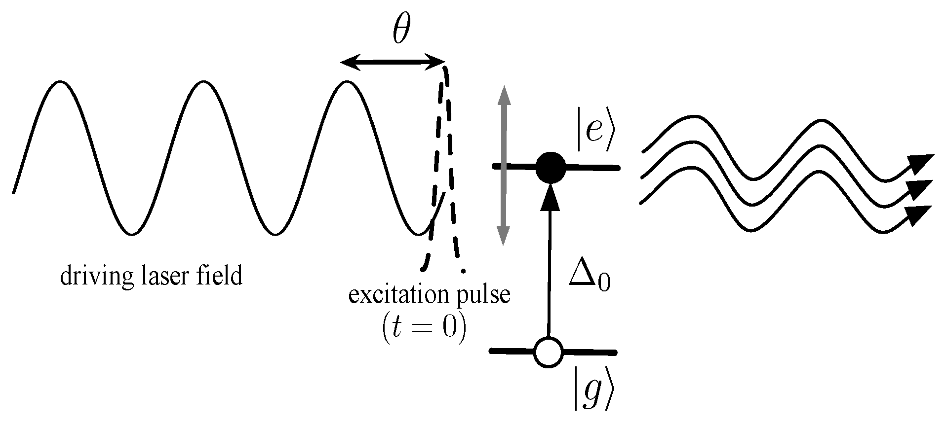
We consider spontaneous emission from a TLS excited by a delta-function pulse. The excited TLS is driven by a monochromatic phase-locked laser field with amplitude and frequency with a phase relative to the excitation delta-pulse as shown in Figure 1. Starting from the minimal coupling Hamiltonian under the dipole approximation, the total Hamiltonian, composed of the electronic system and the radiation field, is represented by [31].
Conversely, the scattered bosonic radiation field is dealt with quantum mechanically: () represents the free radiation field with energy , and is a dimensionless coupling constant, where we consider . The coupling coefficient is given by except for a constant factor [31].
As shown in Appendix A, under the condition of
the Hamiltonian can be written in terms of the adiabatic basis of and given in Equation (A12). Under the rotating wave approximation, the Hamiltonian is given by
where we have defined the renormalized amplitude as
In this paper, we consider a one-dimensional system for simplicity, which does not influence our main results. Hereafter, we simply write as .
Because the number of elementary excitations does not change in , the evolution of the state is closed in a single-excitation subspace of the dressed atom states of and [49]. Then, the Hamiltonian in this subspace is represented by
where the energy difference is defined by , and we take as the origin of energy. In terms of the renormalized amplitude, the intensity of the driving field is given by , so that the maximum intensity is .
Because the Hamiltonian is time-periodic, with , the Floquet theorem may be applied: the wave vector can be written as
with a periodic Floquet eigenfunction with the Floquet quasi-energy [50,51,52]. The composite space is made up of the configuration space and the space of periodic functions in time with period T [50]. The conjugate basis set to the time basis set is constructed as
where [53]. It is well known that the Floquet eigenstate possesses mode-translational symmetry [50]
where denotes the Floquet mode index and classifies a state within a Floquet mode space of .
In terms of the conjugate basis set, the Floquet Hamiltonian is represented by
where denotes the vector in the composite space .
In Equation (10), the first two terms represent the strong coupling between the TLS and the driving field in the Floquet composite basis. We note that the first two terms can be diagonalized in terms of the Wannier-Stark basis [50] given by
where is the n-th order Bessel function of the first kind and . Please note that the Stark state is represented as a coherent sum of the bare discrete states in terms of the Floquet modes. Then, the Floquet Hamiltonian can be rewritten as
where the first and second terms represent the diagonal Floquet energies for the Stark states and the continuous states, respectively. The last term of Equation (12) shows that that the TLS couples with the radiation field with different Floquet modes and the nonlinear interaction depends on the initial phase of the driving field. Please note that this coupling represented by the Bessel function is nonlinear in terms of the driving field amplitude a.
3. Complex Eigenvalue Problem of the Floquet Hamiltonian
The original time-dependent problem now becomes a time-independent eigenvalue problem, where we may employ the established method to solve the complex eigenvalue problem of the Hamiltonian. The difficulty arises, however, when we try to solve the eigenvalue problem by keeping the unstable discrete states in the spectrum in ordinary Hilbert space in the composite space because of the resonance singularity in the interaction between the TLS and the free radiation field [54].
To solve the problem of the resonance singularity, we extend the eigenvector subspace to the extended Hilbert space, where the norm of the eigenvector vanishes [41,42,44,46,47,48,55]. The complex eigenvalue problems of read
where the right-eigenstate and left-eigenstate have the same complex eigenvalue .
The complex eigenbasis of and satisfy the bi-completeness and bi-orthonormal relation [41,46,53]:
where is the Kronecker delta.
The eigenvalue problem of the Floquet Hamiltonian was solved in terms of the Brillouin–Wigner–Feshbach projection method, as shown in Appendix B [46,47,48,53].
In the weak coupling case , the right-resonance eigenstate is given by
where the + sign in the denominator of Equation (16) indicates the analytic continuation of z from the upper half of the complex energy plane [41]. The second term of the curl bracket shows that the resonance states are given by the superposition of the discrete Stark state and the free radiation field belonging to the different Floquet modes with the laser phase-dependent weighted sum of the Bessel function. The left-resonance eigenstates are also obtained by first taking the Hermite conjugate, and then the same analytic continuation with the + index instead of the opposite analytic continuation [41,46,53]. The complex eigenvalue of the resonance state is obtained by solving the nonlinear dispersion equation
where the dynamical self-energy is defined by Equation (A17) and the scalar self-energy function is given by Equation (A18). Of special importance is the fact that the self-energy in the right-hand-side depends on the eigenvalues, which originate in the nonlinearity of the eigenvalue problem of the effective Hamiltonian, as shown in Equation (A19). It should be emphasized that only if we take into account this nonlinearity will the eigenvalues of the non-Hermitian effective Hamiltonian coincide with the Hermitian total Hamiltonian [41]. We have solved this dispersion equation iteratively to obtain the complex eigenvalues of the Floquet Hamiltonian, and we have thereby considered the nonlinearity of the eigenvalue problem of the effective Hamiltonian, as shown in Equation (A14). The resonance state decays exponentially, with the decay rate given by the imaginary part of .
The dressed continuous right-eigenstates are also obtained in Appendix B.2 as
where is the dynamical self-energy, defined by Equation (A17), with the delayed analytic continuation from the upper half plane [41,46]. The continuous left-eigenstate has been similarly obtained without taking the delayed analytic continuation. The dressed continuous right-eigenstate and the left-eigenstate have the same real eigenvalues of that is equivalent to unperturbed energy. The right- and left-eigenstates of the resonance states and the dressed continuous states satisfy the bi-completeness relation in the composite space as
This decomposition of the identity makes it possible to represent any state vector of the total system in terms of the complex spectral expansion.
Using Equation (14), the state vector at time t in the space is given by the Floquet eigenstates as [50]
where we have used the Floquet mode-translational symmetry Equation (9). Using Equation (19), the state vector is given by
It should be noted that the wave function of the emitted single photon is described as the superposition of the single photon states with different frequencies, as shown in the second term of Equation (23).
4. HHG Spectrum
In this work, the HHG spectrum is studied in the case where the TLS is excited from to at by a single-photon pulse. In this case, the spontaneous HHG single-photon emission spectrum, defined as the probability of detecting an emitted photon with frequency during the observation interval t, is obtained by
with [31,56,57]. Substituting the right- and left-eigenstates of in Equation (23), the analytical expression for the spectral amplitude is obtained as
where is the density of states of the free radiation field, and with .
Equation (25) is the principal result of this paper: the contributions of the resonance state and the dressed continuous states are analytically decomposed in the first () and second () terms, respectively. While the first term decays exponentially with time, the second term does not decay over time, giving a stationary HHG spectrum. The third term () represents the branch point effect [41,44], where the contour of the integral denoted by is taken in the different Riemann sheets at the branch point. This term represents the non-Markovian effect, only contributing to the very short time known as Zeno time, or the very long time known as the long-time tale [44]. The contribution of the third term is very small in the present case, with a large amplitude of the driving laser field.
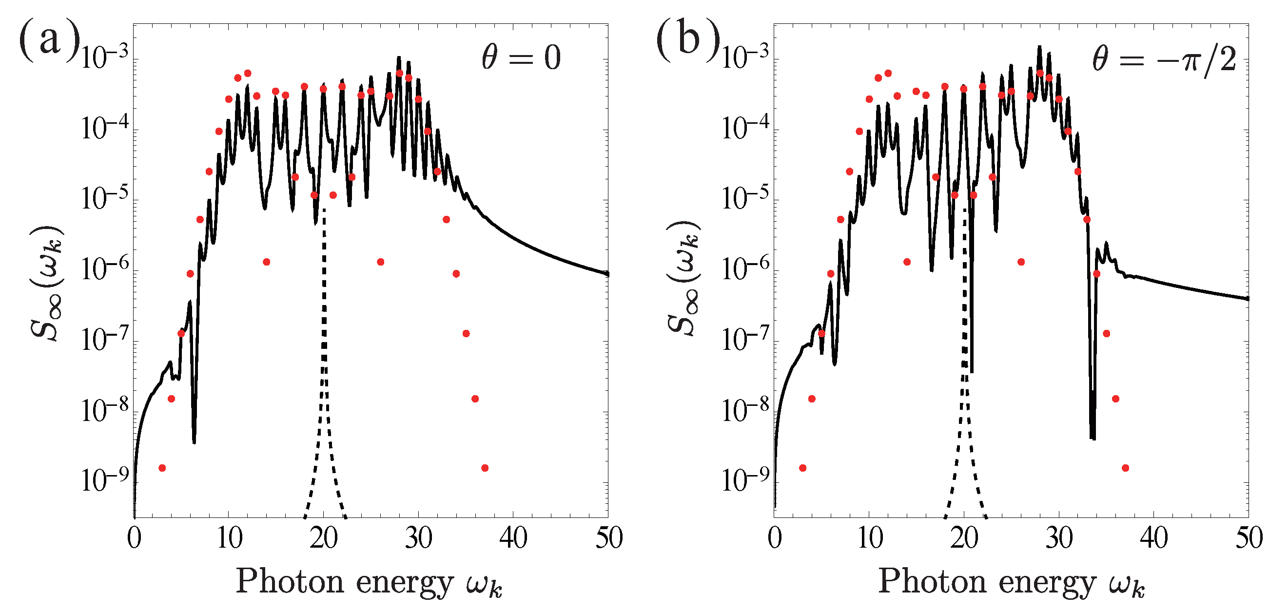
In Figure 2, we show the calculated results of the long-time HHG spectrum for the following parameters: , and in (a) and in (b). We take these parameters to approximately represent the experiments of WSe, such as the driving laser field frequency THz, the band gap between the valence and the conduction bands THz [27]. The driving laser amplitude is determined so as to agree with the cutoff energy of the experiments .
The intensity of the mth-order high-harmonics of the long-time HHG spectrum is mostly determined by the absolute values of the Bessel function , as shown by the red marks in the figures. The characteristic features of the HHG spectrum, such as the plateau and cutoff, are explained by the behavior of the Bessel functions. Because the ratio of the successive order of the Bessel function is evaluated as for , the intensity of the high-harmonics sharply drops at . Consequently, the cutoff energy is determined by the amplitude of the laser field a, and not by the intensity , underlining the typical feature of the HHG spectrum from solids [17,18,19,21].
The cross terms of the different Floquet modes in represent the quantum interferences of the photon emissions from them. Because of this interference effect, Fano-type dip structures appear in the plateau region, as shown in Figure 2. Because the coefficients in the summation in Equation (25) include the initial phase of the laser, the spectral profile of the stationary HHG spectrum is also affected, as shown in Figure 2a,b. Hence, it is possible to quantum mechanically control the HHG photon emission by changing the initial phase of the driving laser field.
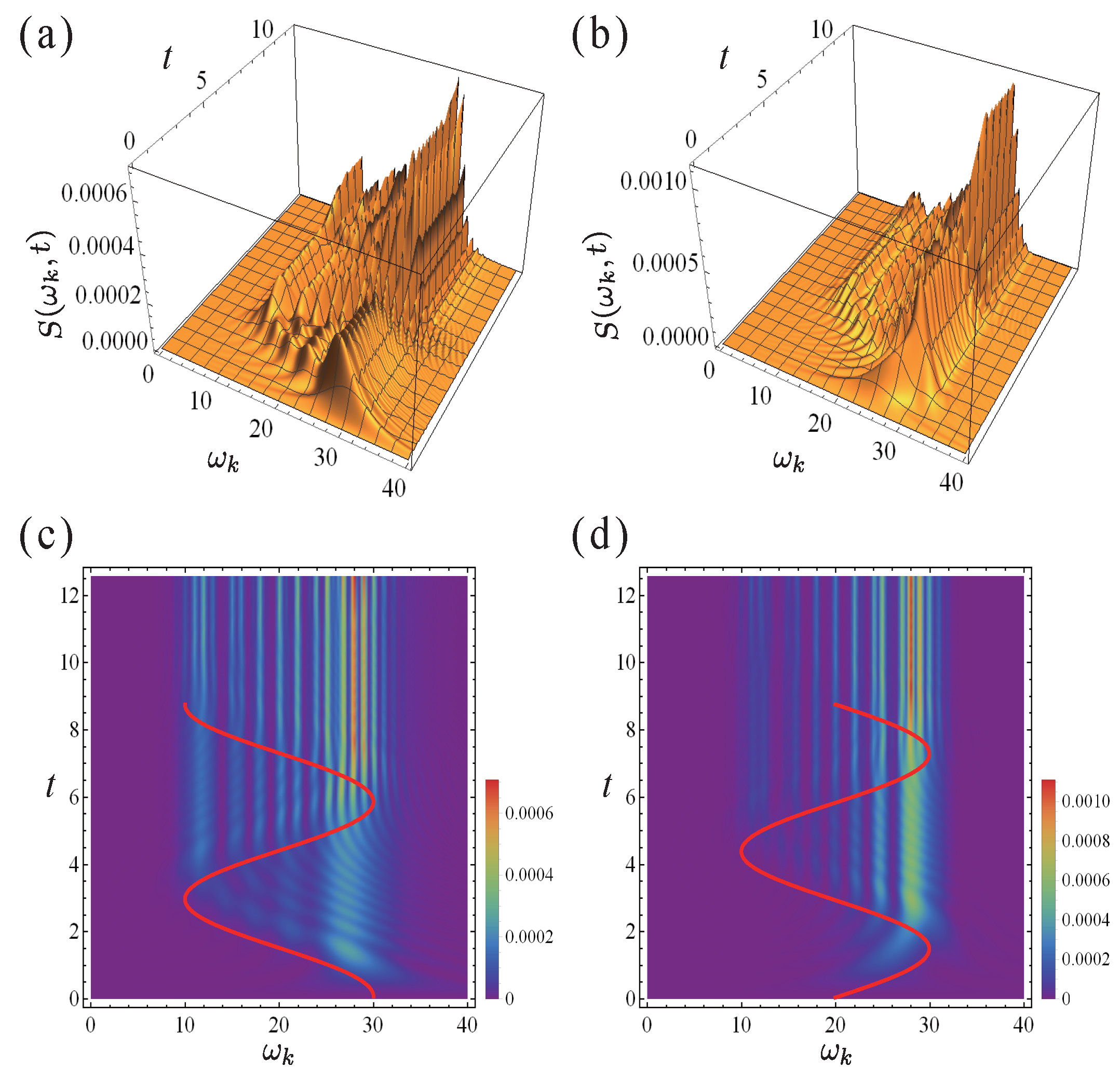
Within the decay time of an excited state, the resonance state components crucially contribute to the temporal profile of the HHG spectrum. As seen from Equation (25) the first and second terms have opposite signs; hence, the spectral amplitude cancels out at , except for the small branch point effect. As the resonance component decays exponentially with time, the spectral cancellation weakens, approaching the stationary HHG spectrum. In Figure 3, the temporal change of the HHG spectrum is shown, where the components of the resonance and dressed-continuous states are separately depicted. Although spectral cancellation of the resonance and dressed field states has been studied in configurational space for a simple spontaneous emission system [44], the present result demonstrates spectral cancellation in the frequency domain under a strong driving field.
The resonance state components of the HHG not only reduce its intensity in time, but also change its spectral shape as a result of the interference of the Floquet resonance modes, as shown by the blue curves in Figure 3, while the dressed-continuous state components retain their spectral shape. Because of the interference of the Floquet resonance states, the peak position of the HHG spectrum adiabatically follows the temporal excited state energy , as shown in Figure 4. In time, the adiabatic behavior of the transient HHG asymptotically approaches the stationary HHG spectrum.
5. Concluding Remarks
We have studied the HHG from a TLS driven by a monochromatic phase-locked laser field in terms of complex spectral analysis for the total system, including the free radiation field, where we have treated the spontaneous HHG photon emission as a coherent quantum process. We have obtained the complex eigenstates of the Floquet Hamiltonian in the extended Hilbert space with the use of the Wannier–Stark basis, going far beyond the ordinary perturbation method. The decomposition of the identity in the extended Hilbert space is represented by the exponentially decaying Floquet resonance states, with complex eigenvalues, and the stable dressed radiation field, with real eigenvalues. These eigenstates are written as a superposition of the different Floquet mode states. The time evolution of the quantum state is then described by the eigenstate expansion of the total system; thereby, the quantum coherence is retained.
We have obtained the analytical expression of the time-frequency resolved spectral amplitude for a HHG single-photon observation. The amplitude is decomposed into the Floquet resonance states and the dressed radiation field, where the former and the latter give the transient and the long-time HHG spectra, respectively. The calculated long-time spectrum shows a typical HHG spectral feature with the plateau and the cutoff, where the spectral cutoff is not proportional to the driving field intensity but the amplitude, as seen in the HHG from solids [17,18,19,20,21]. It is interesting to see that the simple TLS system captures the characteristics of the HHG from solids that possess various electronic excitations. It is likely that the two-level state excitation corresponds to the optically allowed excitation at the point from a valence band to a conduction band [58,59].
Recent experiments have observed multiple plateau structures in the HHG spectrum from solids as a consequence of the quantum interference of the different electronic excitations in solids [18,19]. In this work, we have revealed the other type of quantum interference in the HHG process: the Fano interference between the different Floquet modes, i.e., different high-order harmonics. This quantum interference is caused when a single emitted photon with different frequencies interferes via a common free radiation field, similar to the quantum interference involving different energy states of a single quanta of light [60,61]. This type of interference might be smeared out under a phenomenological assumption.
Within the decay time, the Floquet resonance states contribute to the transient behavior of the HHG spectrum. The transient HHG spectrum changes as if a photon emission occurs from the driven excited state, and the emitted photon energy adiabatically follows the temporal change of the excitation energy. We have shown that this temporal behavior of HHG is understood as a result of the quantum interference between the Floquet resonance states and the dressed field states. Our calculation also shows that the spectrum asymptotically approaches the long-time HHG spectrum, as the resonance state contribution decays exponentially over time.
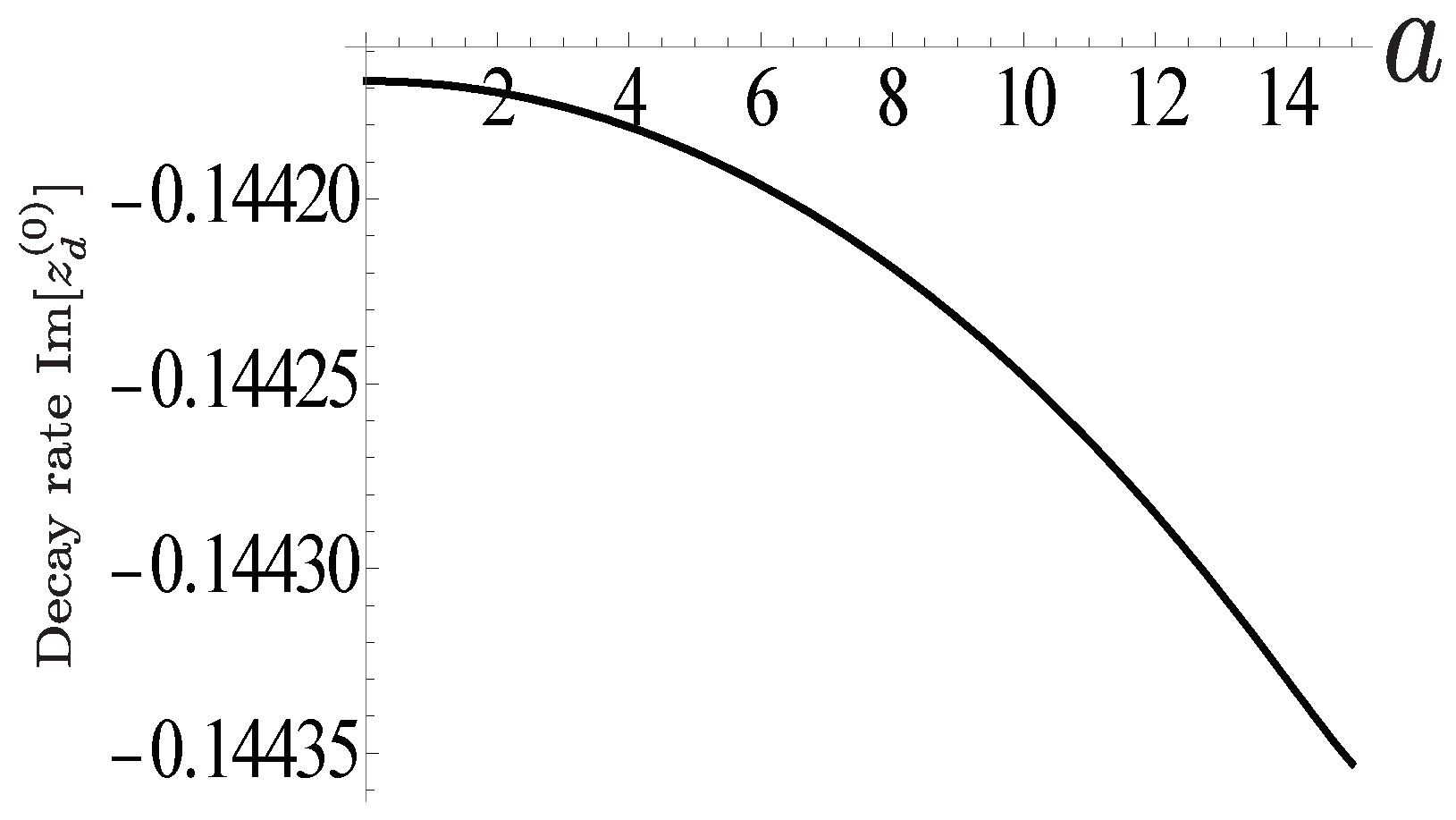
In the present method, the decay process of the excited state is consistently described with the HHG process because the whole process is treated as a coherent quantum process. We find that the decay rate increases with the amplitude of the driving field, as shown in Figure A1. This is because more Floquet resonance is involved in the decaying process as the amplitude of the driving field increases. In our calculation of the HHG spectrum, we have used the decay rate , which corresponds to the lifetime of the excited state of 22 fs. (Please note that the radiative lifetime is considered to be much longer than this value [62]). This is much shorter than the pulse width of the driving laser used in the experiments (≃100 fs) [27]. As long as the pulse width of the driving field is longer than the lifetime of the excited state, the HHG spectrum does not depend on its pulse width.
The conventional theories of the HHG are attempting to solve the time-dependent coupled Schrödinger equation of the electron and the radiation field as an initial value problem [31,37,57]. The problem with these theories is the validity of the Markovian approximation in deriving the kinetic equation of the electron, as its applicability remains uncertain for the far-from-equilibrium situation caused by the driving field [63]. Conversely, the present method attempts to solve the stationary eigenvalue problem in the Floquet space, independent of the initial condition [46,53], where the irreversible time-symmetry breaking is not derived as a result of the Markov approximation for the equation but as a rigorous result of the dynamics caused by the resonance singularity [41,42,44,55]. The present method is an extension of the complex eigenvalue problem of the total Hamiltonian to the Floquet space. Because we have dealt with the HHG photon emission as a coherent quantum process including the radiation field, we may study the time evolution of the quantum coherence of a single photon with different modes , in terms of which we analyze the creation of the quantum coherence through the nonlinear interaction of the electron and the driving field.
In this work, we have assumed the delta-pulse for the excitation pump pulse, which equally excites all the Floquet modes by white excitation. In a real situation, the excitation pulse has a finite pulse width that is as long as 10∼100 fs. It will be interesting to study the effect of a finite pulse width of the excitation, whereby the frequency correlation between the excitation light and the HHG photon can be clarified. Another interesting subject is the competition between the Raman scattering process and the luminescence process in coherent resonant scattering spectroscopy under an intense driving laser field [64,65,66,67]. A study of the effect of the excitation pulse width on the HHG is now underway.
Author Contributions
H.Y. did theoretical analyses and numerical calculations, and wrote the first draft. S.T. supervised this program and finalized the manuscript.
Funding
This research was funded by JSPS KAKENHI grants number JP16H04003, No. JP16K05481, and No. JP17K05585.
Acknowledgments
We are very grateful T. Petrosky, K. Noba, K. Kanki, S. Garmon, Y. Kayanuma, and M. Domina for fruitful discussions.
Conflicts of Interest
The authors declare no conflict of interest. The founding sponsors had no role in the design of the study; in the collection, analyses, or interpretation of data; in the writing of the manuscript, and in the decision to publish the results.
Abbreviations
The following abbreviations are used in this manuscript:
| HHG | High-Harmonic Generation |
| TLS | Two-Level System |
| CEP | Carrier-Envelope-Phase |
Appendix A. Hamiltonian of the Driven TLS
In this section, we shall derive the driven TLS Hamiltonian Equation (4) starting from an off-diagonal coupling of the TLS with the radiation field.
We consider spontaneous photon emission from a driven two-level system (TLS) consisting of the ground state and an excited state with the excitation energy . The TLS is driven energetically by a monochromatic phase-locked laser field, as shown in Figure 1. The TLS is excited from the ground state to the excited state at by a delta-function pulse, followed by spontaneous emission under the energy driving. The Hamiltonian is given by Equation (1):
We solve the adiabatic eigenvalue problem of the driven TLS:
The adiabatic eigenvalues are given by
and the corresponding eigenstates are
where
We consider the situation where the energy gap between the ground state and the excited state is much larger than the amplitude of the driving field:
and the amplitude is much larger than the energy quanta of the driving field,
Under these conditions, we can rewrite in terms of the adiabatic eigenstates as
Shifting the energy origin to , we have
With the use of the rotating wave approximation for the TLS and the free radiation field and defining
we have
With the definition of Equation (A11), the above conditions for Equations (A7) and (A8) reduce to Equation (3).
Appendix B. Complex Eigenvalue Problem of the Floquet Hamiltonian
Appendix B.1. Discrete Floquet Resonance State
To solve the complex eigenvalue problem for the atom in the -space, we use the Feshbach—Brilloiun–Wigner projection method with the projection operators
where is the projection operators on the Stark basis set . Acting these projection operators on Equation (13), we have a closed form of the eigenvalue problem of the effective Hamiltonian in the P-subspace as
where the effective Hamiltonian is given by
The dynamical self-energy is given by
with the self-energy represented as the Cauchy integral,
Because of the resonance singularity in the self-energy, the effective Hamiltonian becomes non-Hermitian with the complex eigenvalues. We would emphasize that the eigenvalue problem is nonlinear because the effective Hamiltonian depends on its own eigenvalue in the eigenvalue problem Equation (A19). When this nonlinearity is taken into account, the eigenvalues of the effective Hamiltonian are the same as those of the total Hamiltonian [41,47].
In our previous work, we have solved the eigenvalue problem of the Floquet Hamiltonian using the continued fraction expansion [46]; here, the strong coupling with the driving field has been fully incorporated in the Stark basis. With the Floquet translational symmetry Equation (9), it is enough to consider the eigenstates for the principal mode . In the week coupling case , we can neglect the off-diagonal component of so that the eigenvalue problem of has been solved as
where the complex eigenvalue of the resonance state is obtained by iteratively solving the nonlinear dispersion equation
The imaginary part of is given by the decay rate of the excited state.
It should be noted that the decay rate is given by the weighted sum of the self-energy with the Bessel function. In Figure A1, we show the calculated results of the decay rate as a function of . It can be shown that if the bandwidth of the free radiation field is on the same order as , such as for a photonic crystal, the decay rate may completely vanish as the coherent destruction tunneling from to [46].
Figure A1.
as a function of the driving field amplitude for , , .
Now that we have solved the eigenvalue problem of in the P-subspace, the eigenstate of the total Hamiltonian with the same eigenvalue is obtained by adding the Q-component.
where we take the analytic continuation toward these complex poles from the upper complex plane in the Cauchy integral [41]. The left resonance state is similarly obtained as
where it should be noted that we need to take the same direction in the analytic continuation of the Cauchy integral as with the right-resonance state to obtain the same complex eigenvalue.
The normalization constants of and are determined so as to satisfy the bi-normalization condition of
With use of Equations (A17), (A21), and (A22), the bi-normalization condition reads
Appendix B.2. Dressed Radiation Field
We take the same procedure for the radiation field of the Floquet Hamiltonian. The projection for the continuum state is taken as
The effective Hamiltonian can be obtained as with the resonant state,
Therefore, we get the eigenvalue problem of the effective Hamiltonian (A27)
We have obtained the expression for the dressed radiation field as
where Green’s function is determined by
In the weak coupling case, we may neglect the off-diagonal terms, approximating
Therefore, we finally obtain
which give Equation (18).
References
- Corkum, P.B.; Krausz, F. Attosecond science. Nat. Phys. 2007, 3, 381–387. [Google Scholar] [CrossRef]
- Krausz, F.; Ivanov, M. Attosecond physics. Rev. Mod. Phys. 2009, 81, 163–234. [Google Scholar] [CrossRef]
- Corkum, P.; Burnett, N.; Brunel, F. Above-threshold ionization in the long-wavelength limit. Phys. Rev. Lett. 1989, 62, 1259–1262. [Google Scholar] [CrossRef] [PubMed]
- Mohideen, U.; Sher, M.; Tom, H.; Aumiller, G.; Wood, O.; Freeman, R.; Boker, J.; Bucksbaum, P. High intensity above-threshold ionization of He. Phys. Rev. Lett. 1993, 71, 509–512. [Google Scholar] [CrossRef] [PubMed]
- Corkum, P.B. Plasma perspective on strong field multiphoton ionization. Phys. Rev. Lett. 1993, 71, 1994–1997. [Google Scholar] [CrossRef] [PubMed] [Green Version]
- Schafer, K.J.; Kulander, K.C. High Harmonic Generation from Ultrafast Pump Lasers. Phys. Rev. Lett. 1997, 78, 638–641. [Google Scholar] [CrossRef] [Green Version]
- Krause, J.; Schafer, K.; Kulander, K. High-order harmonic generation from atoms and ions in the high intensity regime. Phys. Rev. Lett. 1992, 68, 3535–3538. [Google Scholar] [CrossRef] [PubMed]
- Brabec, T.; Krausz, F. Intense few-cycle laser fields: Frontiers of nonlinear optics. Rev. Mod. Phys. 2000, 72, 545–591. [Google Scholar] [CrossRef]
- Popmintchev, T.; Chen, M.C.; Arpin, P.; Murnane, M.M.; Kapteyn, H.C. The attosecond nonlinear optics of bright coherent X-ray generation. Nat. Photonics 2010, 4, 822–832. [Google Scholar] [CrossRef]
- Popmintchev, T.; Chen, M.C.; Popmintchev, D.; Arpin, P.; Brown, S.; Ališauskas, S.; Andriukaitis, G.; Balčiunas, T.; Mücke, O.D.; Pugzlys, A.; et al. Bright Coherent Ultrahigh Harmonics in the keV X-ray Regime from Mid-Infrared Femtosecond Lasers. Science 2012, 336, 1287–1291. [Google Scholar] [CrossRef] [PubMed]
- Kim, K.T.; Zhang, C.; Ruchon, T.; Hergott, J.F.; Auguste, T.; Villeneuve, D.M.; Corkum, P.B.; Quéré, F. Photonic streaking of attosecond pulse trains. Nat. Photonics 2013, 7, 651–656. [Google Scholar] [CrossRef]
- Gruson, V.; Barreau, L.; Jiménez-Galan, Á.; Risoud, F.; Caillat, J.; Maquet, A.; Carré, B.; Lepetit, F.; Hergott, J.F.; Ruchon, T.; et al. Attosecond dynamics through a Fano resonance: Monitoring the birth of a photoelectron. Science 2016, 354, 734–738. [Google Scholar] [CrossRef] [PubMed] [Green Version]
- Kaldun, A.; Blättermann, A.; Stooß, V.; Donsa, S.; Wei, H.; Pazourek, R.; Nagele, S.; Ott, C.; Lin, C.D.; Burgdörfer, J.; et al. Observing the ultrafast buildup of a Fano resonance in the time domain. Science 2016, 354, 738–741. [Google Scholar] [CrossRef] [PubMed]
- Cirelli, C.; Marante, C.; Heuser, S.; Petersson, C.; Galán, Á.; Argenti, L.; Zhong, S.; Busto, D.; Isinger, M.; Nandi, S.; et al. Anisotropic photoemission time delays close to a Fano resonance. Nat. Commun. 2018, 9. [Google Scholar] [CrossRef] [PubMed]
- Nisoli, M.; Decleva, P.; Calegari, F.; Palacios, A.; Martín, F. Attosecond Electron Dynamics in Molecules. Chem. Rev. 2017, 117, 10760–10825. [Google Scholar] [CrossRef] [PubMed]
- Young, L.; Ueda, K.; Gühr, M.; Bucksbaum, P.; Simon, M.; Mukamel, S.; Rohringer, N.; Prince, K.; Masciovecchio, C.; Meyer, M.; et al. Roadmap of ultrafast x-ray atomic and molecular physics. J. Phys. B 2018, 51. [Google Scholar] [CrossRef]
- Ghimire, S.; Dichiara, A.; Sistrunk, E.; Agostini, P.; Dimauro, L.; Reis, D. Observation of high-order harmonic generation in a bulk crystal. Nat. Phys. 2011, 7, 138–141. [Google Scholar] [CrossRef]
- Schubert, O.; Hohenleutner, M.; Langer, F.; Urbanek, B.; Lange, C.; Huttner, U.; Golde, D.; Meier, T.; Kira, M.; Koch, S.W.; et al. Sub-cycle control of terahertz high-harmonic generation by dynamical Bloch oscillations. Nat. Photonics 2014, 8, 119–123. [Google Scholar] [CrossRef] [Green Version]
- Hohenleutner, M.; Langer, F.; Schubert, O.; Knorr, M.; Huttner, U.; Koch, S.; Kira, M.; Huber, R. Real-time observation of interfering crystal electrons in high-harmonic generation. Nature 2015, 523, 572–575. [Google Scholar] [CrossRef] [PubMed] [Green Version]
- Vampa, G.; Hammond, T.; Thiré, N.; Schmidt, B.; Légaré, F.; McDonald, C.; Brabec, T.; Corkum, P. Linking high harmonics from gases and solids. Nature 2015, 522, 462–464. [Google Scholar] [CrossRef] [PubMed]
- Ndabashimiye, G.; Ghimire, S.; Wu, M.; Browne, D.A.; Schafer, K.J.; Gaarde, M.B.; Reis, D.A. Solid-state harmonics beyond the atomic limit. Nature 2016, 534, 520–523. [Google Scholar] [CrossRef] [PubMed]
- Bauer, D.; Hansen, K.K. High-Harmonic Generation in Solids with and without Topological Edge States. Phys. Rev. Lett. 2018, 120, 177401. [Google Scholar] [CrossRef] [PubMed] [Green Version]
- McDonald, C.R.; Amin, K.S.; Aalmalki, S.; Brabec, T. Enhancing High Harmonic Output in Solids through Quantum Confinement. Phys. Rev. Lett. 2017, 119, 183902. [Google Scholar] [CrossRef] [PubMed]
- Luu, T.T.; Garg, M.; Kruchinin, S.Y.; Moulet, A.; Hassan, M.T.; Goulielmakis, E. Extreme ultraviolet high-harmonic spectroscopy of solids. Nature 2015, 521, 498–502. [Google Scholar] [CrossRef] [PubMed]
- You, Y.S.; Yin, Y.; Wu, Y.; Chew, A.; Ren, X.; Zhuang, F.; Gholam-Mirzaei, S.; Chini, M.; Chang, Z.; Ghimire, S. High-harmonic generation in amorphous solids. Nat. Commun. 2017, 8, 724. [Google Scholar] [CrossRef] [PubMed] [Green Version]
- Zaks, B.; Liu, R.B.; Sherwin, M.S. Experimental observation of electron–hole recollisions. Nature 2012, 483, 580–583. [Google Scholar] [CrossRef] [PubMed]
- Langer, F.; Hohenleutner, M.; Schmid, C.P.; Poellmann, C.; Nagler, P.; Korn, T.; Schüller, C.; Sherwin, M.S.; Huttner, U.; Steiner, J.T.; et al. Lightwave-driven quasiparticle collisions on a subcycle timescale. Nature 2016, 533, 225–229. [Google Scholar] [CrossRef] [PubMed] [Green Version]
- Uchida, K.; Otobe, T.; Mochizuki, T.; Kim, C.; Yoshita, M.; Akiyama, H.; Pfeiffer, L.N.; West, K.W.; Tanaka, K.; Hirori, H. Subcycle Optical Response Caused by a Terahertz Dressed State with Phase-Locked Wave Functions. Phys. Rev. Lett. 2016, 117, 277402. [Google Scholar] [CrossRef] [PubMed] [Green Version]
- Uchida, K.; Otobe, T.; Mochizuki, T.; Kim, C.; Yoshita, M.; Tanaka, K.; Akiyama, H.; Pfeiffer, L.N.; West, K.W.; Hirori, H. Coherent detection of THz-induced sideband emission from excitons in the nonperturbative regime. Phys. Rev. B 2018, 97, 165122. [Google Scholar] [CrossRef]
- Luu, T.; Wörner, H. High-order harmonic generation in solids: A unifying approach. Phys. Rev. B 2016, 94. [Google Scholar] [CrossRef] [Green Version]
- Milonni, P.W. The Quantum Vacuum: An Introduction to Quantum Electrodynamics; Academic Press: New York, NY, USA, 1994. [Google Scholar]
- Mukamel, S. Principles of Nonlinear Optical Spectroscopy; Oxford Series in Optical and Imaging Sciences; Oxford University Press: Oxford, UK, 1995. [Google Scholar]
- Kulander, K.C.; Schafer, K.J. Time-dependent calculations of electron and photon emission from an atom in an intense laser field. In Atoms and Molecules in Intense Fields; Springer: Berlin/Heidelberg, Germany, 1997; pp. 149–172. [Google Scholar]
- Tancogne-Dejean, N.; Mücke, O.D.; Kärtner, F.X.; Rubio, A. Impact of the Electronic Band Structure in High-Harmonic Generation Spectra of Solids. Phys. Rev. Lett. 2017, 118, 087403. [Google Scholar] [CrossRef] [PubMed]
- Vampa, G.; McDonald, C.R.; Orlando, G.; Corkum, P.B.; Brabec, T. Semiclassical analysis of high harmonic generation in bulk crystals. Phys. Rev. B 2015, 91, 064302. [Google Scholar] [CrossRef] [Green Version]
- Golde, D.; Meier, T.; Koch, S.W. High harmonics generated in semiconductor nanostructures by the coupled dynamics of optical inter- and intraband excitations. Phys. Rev. B 2008, 77, 075330. [Google Scholar] [CrossRef]
- Weisskopf, V.; Wigner, E. Berechnung der natürlichen Linienbreite auf Grund der Diracschen Lichttheorie. Zeitschrift für Physik 1930, 63, 54–73. [Google Scholar] [CrossRef]
- Heitler, W. The Quantum Theory of Radiation; International Series of Monographs on Physics; Oxford University Press: Oxford, UK, 1947. [Google Scholar]
- Compagno, G.; Passante, R.; Persico, F. Atom-Field Interactions and Dressed Atoms; Cambridge Studies in Modern Optics; Cambridge University Press: Cambridge, UK, 1995. [Google Scholar]
- Cohen-Tannoudji, C.; Dupont-Roc, J.; Grynberg, G. Atom—Photon Interactions: Basic Process and Applications. In Atom—Photon Interactions; Wiley: Weinheim, Germany, 2008. [Google Scholar]
- Petrosky, T.; Prigogine, I.; Tasaki, S. Quantum theory of non-integrable systems. Phys. A Stat. Mech. Appl. 1991, 173, 175–242. [Google Scholar] [CrossRef]
- Petrosky, T.; Prigogine, I. The Liouville space extension of quantum mechanics. Adv. Chem. Phys. 1997, 99, 1–120. [Google Scholar]
- Ordonez, G.; Petrosky, T.; Prigogine, I. Quantum transitions and dressed unstable states. Phys. Rev. A 2001, 63, 052106. [Google Scholar] [CrossRef]
- Petrosky, T.; Ordonez, G.; Prigogine, I. Space-time formulation of quantum transitions. Phys. Rev. A 2001, 64, 062101/1–062101/21. [Google Scholar] [CrossRef]
- Tanaka, S.; Garmon, S.; Petrosky, T. Nonanalytic enhancement of the charge transfer from adatom to one-dimensional semiconductor superlattice and optical absorption spectrum. Phys. Rev. B 2006, 73, 115340. [Google Scholar] [CrossRef]
- Yamada, N.; Noba, K.I.; Tanaka, S.; Petrosky, T. Dynamical suppression and enhancement of instability for an unstable state by a periodic external field. Phys. Rev. B 2012, 86. [Google Scholar] [CrossRef]
- Tanaka, S.; Garmon, S.; Kanki, K.; Petrosky, T. Higher-order time-symmetry-breaking phase transition due to meeting of an exceptional point and a Fano resonance. Phys. Rev. A 2016, 94, 022105. [Google Scholar] [CrossRef]
- Fukuta, T.; Garmon, S.; Kanki, K.; Noba, K.i.; Tanaka, S. Fano absorption spectrum with the complex spectral analysis. Phys. Rev. A 2017, 96, 052511. [Google Scholar] [CrossRef]
- Cohen-Tannoudji, C.; Dupont-Roc, J.; Grynberg, G. Atom-Photon Interactions: Basic Processes and Applications; Wiley: Hoboken, NJ, USA, 1998. [Google Scholar]
- Grifoni, M.; Hänggi, P. Driven quantum tunneling. Phys. Rep. 1998, 304, 229–354. [Google Scholar] [CrossRef] [Green Version]
- Shirley, J. Solution of the schrödinger equation with a hamiltonian periodic in time. Phys. Rev. 1965, 138, B979–B987. [Google Scholar] [CrossRef]
- Sambe, H. Steady states and quasienergies of a quantum-mechanical system in an oscillating field. Phys. Rev. A 1973, 7, 2203–2213. [Google Scholar] [CrossRef]
- Yamane, H.; Tanaka, S.; Domina, M.; Passante, R.; Petrosky, T. Analysis of high-harmonic generation in terms of complex Floquet spectral analysis. In Proceedings of the 2017 Progress in Electromagnetics Research Symposium, Singapore, 19–22 November 2017; pp. 1437–1444. [Google Scholar]
- Friedrichs, K. On the perturbation of continuous spectra. Commun. Pure Appl. Math. 1948, 1, 361–406. [Google Scholar] [CrossRef]
- Petrosky, T.; Ordonez, G.; Prigogine, I. Quantum transitions and nonlocality. Phys. Rev. A 2000, 62, 042106. [Google Scholar] [CrossRef]
- Glauber, R.J. Optical Coherence and Photon Statistics. In Quantum Theory of Optical Coherence; de Witt, C., Blandin, A., Cohen-Tannoudji, C., Eds.; WileyWiley: Hoboken, NJ, USA, 2007; Chapter 2; pp. 23–182. [Google Scholar]
- Carmichael, H. Statistical Methods in Quantum Optics 1: Master Equations and Fokker-Planck Equations; Theoretical and Mathematical Physics; Springer: Berlin/Heidelberg, Germany, 2013. [Google Scholar]
- Korbman, M.; Kruchinin, S.Y.; Yakovlev, V.S. Quantum beats in the polarization response of a dielectric to intense few-cycle laser pulses. New J. Phys. 2013, 15, 013006. [Google Scholar] [CrossRef] [Green Version]
- Wu, M.; Browne, D.A.; Schafer, K.J.; Gaarde, M.B. Multilevel perspective on high-order harmonic generation in solids. Phys. Rev. A 2016, 94, 063403. [Google Scholar] [CrossRef]
- Clemmen, S.; Farsi, A.; Ramelow, S.; Gaeta, A.L. Ramsey Interference with Single Photons. Phys. Rev. Lett. 2016, 117, 223601. [Google Scholar] [CrossRef] [PubMed]
- Whiting, D.J.; Šibalić, N.; Keaveney, J.; Adams, C.S.; Hughes, I.G. Single-Photon Interference due to Motion in an Atomic Collective Excitation. Phys. Rev. Lett. 2017, 118, 253601. [Google Scholar] [CrossRef] [PubMed]
- Tripathi, L.N.; Iff, O.; Betzold, S.; Dusanowski, Ł.; Emmerling, M.; Moon, K.; Lee, Y.J.; Kwon, S.H.; Höfling, S.; Schneider, C. Spontaneous Emission Enhancement in Strain-Induced WSe2 Monolayer-Based Quantum Light Sources on Metallic Surfaces. ACS Photonics 2018, 5, 1919–1926. [Google Scholar] [CrossRef] [Green Version]
- Browne, D.E.; Keitel, C.H. Resonance fluorescence in intense laser fields. J. Mod. Opt. 2000, 47, 1307–1337. [Google Scholar] [CrossRef]
- Hizhyakov, V.; Tehver, I. Theory of Resonant Secondary Radiation due to Impurity Centres in Crystals. Phys. Status Solidi B 1967, 21, 755–768. [Google Scholar] [CrossRef]
- Toyozawa, Y. Resonance and Relaxation in Light Scattering. J. Phys. Soc. Jpn. 1976, 41, 400–411. [Google Scholar] [CrossRef]
- Kotani, A. On the Relationship between Resonant Light Scattering and Luminescence—A Singular Aspect in Localized Electron-Phonon System with Linear Interaction. J. Phys. Soc. Jpn. 1978, 44, 965–972. [Google Scholar] [CrossRef]
- Kayamura, Y. Resonant Secondary Radiation in Strongly Coupled Localized Electron-Phonon System. J. Phys. Soc. Jpn. 1988, 57, 292–301. [Google Scholar] [CrossRef]
Figure 1.
High-harmonic generation of a driven TLS.

Figure 2.
Stationary HHG spectrum for . (a) and (b) . The fundamental spontaneous emission spectrum at is shown by the dashed lines. The red marks indicate the absolute value of the Bessel function .
Figure 2.
Stationary HHG spectrum for . (a) and (b) . The fundamental spontaneous emission spectrum at is shown by the dashed lines. The red marks indicate the absolute value of the Bessel function .

Figure 3.
The temporal spectral profile of HHG (black line) for (a), (b), (c), and (d), where the same parameters of Figure 2a are used. The resonance state and the dressed continuous state components are depicted by blue and red lines, respectively. The excited state energies are indicated by the arrows.
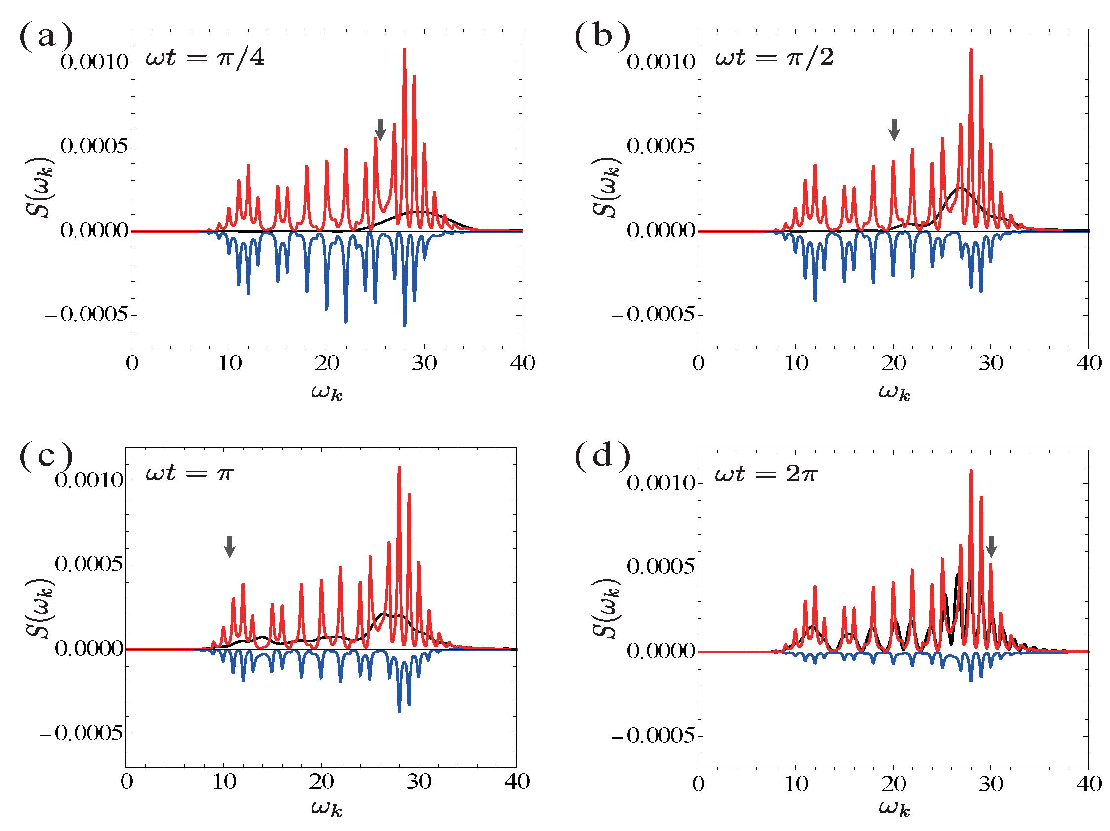
Figure 4.
The transient HHG spectrum for (a,c), and (b,d). The parameters are the same as in Figure 2. The red curves in the contour maps (c,d) indicate .
Figure 4.
The transient HHG spectrum for (a,c), and (b,d). The parameters are the same as in Figure 2. The red curves in the contour maps (c,d) indicate .

© 2018 by the authors. Licensee MDPI, Basel, Switzerland. This article is an open access article distributed under the terms and conditions of the Creative Commons Attribution (CC BY) license (http://creativecommons.org/licenses/by/4.0/).
Share and Cite
MDPI and ACS Style
Yamane, H.; Tanaka, S. Ultrafast Dynamics of High-Harmonic Generation in Terms of Complex Floquet Spectral Analysis. Symmetry 2018, 10, 313. https://0-doi-org.brum.beds.ac.uk/10.3390/sym10080313
AMA Style
Yamane H, Tanaka S. Ultrafast Dynamics of High-Harmonic Generation in Terms of Complex Floquet Spectral Analysis. Symmetry. 2018; 10(8):313. https://0-doi-org.brum.beds.ac.uk/10.3390/sym10080313
Chicago/Turabian StyleYamane, Hidemasa, and Satoshi Tanaka. 2018. "Ultrafast Dynamics of High-Harmonic Generation in Terms of Complex Floquet Spectral Analysis" Symmetry 10, no. 8: 313. https://0-doi-org.brum.beds.ac.uk/10.3390/sym10080313
Note that from the first issue of 2016, this journal uses article numbers instead of page numbers. See further details here.