Equilibrium of Two-Dimensional Cycloidal Pantographic Metamaterials in Three-Dimensional Deformations


International Research Center on Mathematics and Mechanics of Complex Systems—MeMoCS, Università degli studi dell’Aquila, 67100 L’Aquila, Italy
*
Author to whom correspondence should be addressed.
†
These authors contributed equally to this work.
Symmetry 2019, 11(12), 1523; https://0-doi-org.brum.beds.ac.uk/10.3390/sym11121523
Submission received: 17 November 2019
/
Revised: 6 December 2019
/
Accepted: 13 December 2019
/
Published: 16 December 2019
(This article belongs to the Special Issue Recent Advances in the Study of Symmetry and Continuum Mechanics)
Abstract
:A particular pantographic sheet, modeled as a two-dimensional elastic continuum consisting of an orthogonal lattice of continuously distributed fibers with a cycloidal texture, is introduced and investigated. These fibers conceived as embedded beams on the surface are allowed to be deformed in a three-dimensional space and are endowed with resistance to stretching, shearing, bending, and twisting. A finite element analysis directly derived from a variational formulation was performed for some explanatory tests to illustrate the behavior of the newly introduced material. Specifically, we considered tests on: (1) bias extension; (2) compressive; (3) shear; and (4) torsion. The numerical results are discussed to some extent. Finally, attention is drawn to a comparison with other kinds of orthogonal lattices, namely straight, parabolic, and oscillatory, to show the differences in the behavior of the samples due to the diverse arrangements of the fibers.
1. Introduction
In recent decades, metamaterials has attracted the attention of the scientific community considerably. They are artificially constructed materials characterized by an interior architecture that is designed with the aim of producing an optimized combination of responses to specific external excitation. One may conceive many possible metamaterials depending on the particular properties to be obtained. For example, metamaterials may be mechanical, acoustic, electromagnetic, optic, and so on. Typically, metamaterials show qualitative exotic behaviors due to their substructure rather than to the composition of the material of which they are made [1,2,3,4].
In this paper, we investigate a particular type of mechanical metamaterial [5,6,7]: a pantographic sheet [8,9,10,11,12,13,14,15]. This particular material has been introduced as the first synthetic example of material exhibiting a strain–energy function involving second gradient contributions relevant at a macroscopic scale of observation [16,17,18]. This main feature is inherited by the presence of “fibers” that, having a resistance to being bent, require the presence of spatial second-order derivatives of the displacement to properly describe their energy.
It is worth noticing that the pantographic structure may be used as a reinforcement of composite material, e.g., a two-phase continuum with a “pantographic-inspired” architecture, which is a 3D fiber network, surrounded by a matrix, capable of large deformations [19,20,21,22].
From a geometric point of view, a pantographic surface resembles very closely an elastic network structure. Therefore, many of the achievements in modeling these systems can be fruitfully employed also for the pantographic sheets (see, e.g., [23,24,25,26,27,28,29]). According to these results, the pantographic structure is identified with a surface composed of two families of continuously distributed fibers in the framework of continuum theory. Indeed, this kind of perspective is also justified by homogenization procedures applied to the discrete system of fibers [30,31,32,33,34,35,36]. Besides, since the fibers are modeled in accordance with the beam theory, which entails the description of their cross-section rotation, the pantographic sheets may be regarded as micropolar continua. Thus, results from this research topic are available too (see, e.g., [37,38,39]).
For the sake of completeness, we have to mention that pantographic structures, as microstructured materials, may also show impressive dynamical features related to the complexity of the interior architecture [40,41,42,43,44,45]. Besides, in this context of engineered materials, it is also worth mentioning the study of dynamically self-organized “intelligent” materials [46] or functionally graded materials [47].
The paper is organized as follows. Section 2 describes the pantographic system with initially cycloidal fibers. Section 3 is devoted to giving some numerical examples of the behavior of this arrangement of fibers. Finally, Section 4 reports a comparison with other kinds of fiber dispositions and discusses the differences.
2. Pantographic Sheets with Initially Cycloidal Fibers
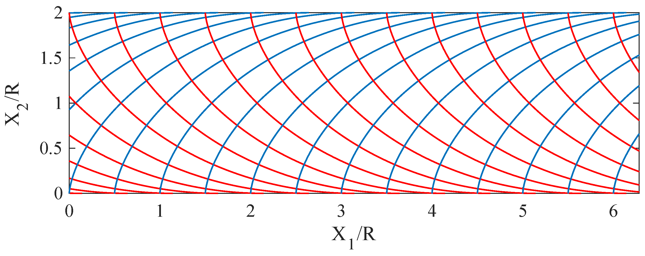
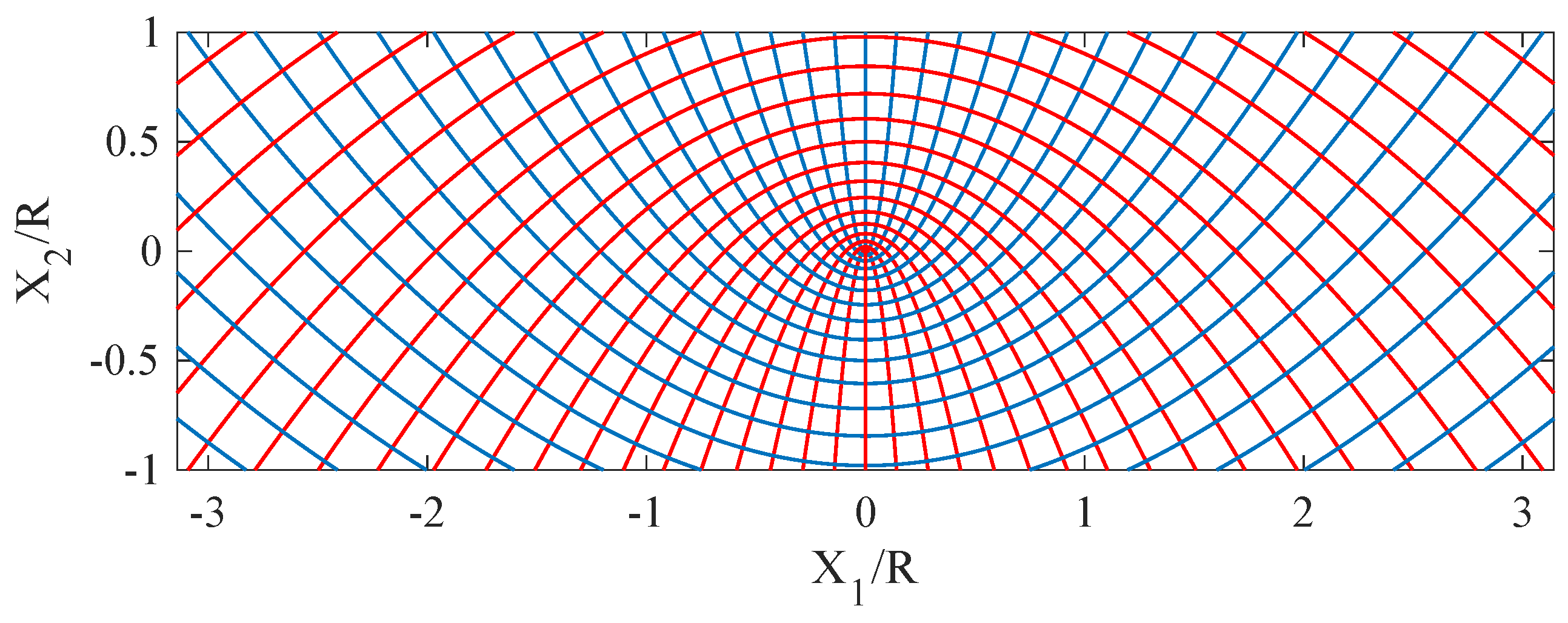
The pantographic sheet investigated is characterized by an orthogonal lattice of fibers initially curved and arranged parallel to two families of cycloids. The sample under study is rectangular and cut suitably in order to have a fiber disposition symmetric with respect to the longitudinal axis of the specimen and with a higher density along the most extended lateral edges. This arrangement of the fibers has been specially conceived with the purpose of employing the superior capability of curved fibers to bear loads (fibers tend to behave like arches) and to have reinforcement in long boundaries (see Figure 1). Therefore, the sample has a notably anisotropic behavior with an extremely soft core (due to the pantographic effect [16,17,48,49,50,51]) and a stiffer part at the borders.
The two families of curves with one parameter, namely and , in an initial rectangular domain of size are represented in Cartesian coordinates, for the first family, as
and, for the second family, as
where and are constants that identify the particular curve belonging to the family.
The deformation of the pantographic surface is defined by the map , which takes the material particle initially placed in and yields the current position of that particle in a three-dimensional Euclidean space.
By assuming a Cartesian coordinate system with and parallel to the edges of the sample, and introducing the components of displacement in that basis, the explicit expression of the placement map becomes
where Greek indexes range from 1 to 2 while Latin ones from 1 to 3. The differentiation with respect to the Cartesian coordinates of is represented by the following notation
Recalling the definition of the deformation gradient , we have
The Cauchy–Green deformation tensor is thus given by
and the strain tensor can be evaluated, by components, as follows
where is the Kronecker delta. The considered problem also needs to explicate the second gradient of the deformation, , namely , because it is able to describe the curvatures and the twist of the fibers [52,53]. Indeed, we recall here that the considered continuous surface can be thought of as an infinite distribution of curved fibers arranged in the domain, as mentioned above (see also [54]), assumed to be material curves with no relative slipping and tied together at their points of intersection.
According to Steigmann and dell’Isola [53], a suitable fiber decomposition is introduced by means of a couple of orthogonal unit vector fields , which determines the fiber directions in the plane of for the reference configuration. Besides, the fibers directions in the current configuration, i.e., after a deformation, are given by the unit vectors as follows
where and are the stretches of fibers. Knowing the current directions of fibers , which define the tangent plane to the deformed pantographic sheet at the material point initially in , it is possible to evaluate the shear distortion angle , i.e., the change of angle passing from to , by
The tangent vector to each curve of the family in Equation (1) is obtained by
Using Equation (1), with simple algebraic calculations, we obtain
and, exploiting the properties of the trigonometric functions,
Choosing a root of Equation (12), the parameter can be expressed in terms of Cartesian coordinates as follows
therefore, the tangent vector to any curve of the family in Equation (1) at the point , in Cartesian coordinates, becomes
and its norm is
Eventually, the unit vectors and are
In Equations (16), we take advantage of the fact that the two families of curves in Equations (1) and (2) are orthogonal in the intersection point. Alternatively, may be evaluated with the same strategy used for applied to the curves in Equation (2).
Using the fiber decomposition previously defined, the gradient of deformation is
thereby the Cauchy–Green deformation tensor takes the expression:
and the second gradient of the deformation becomes [53]
where
and
and being the geodesic curvatures of the deformed fibers, namely the part of the fiber curvatures in the tangent plane of the deformed sheet, and and the so-called Tchebychev curvatures. Besides,
define the orthogonal directions of the fibers embedded on the pantographic sheet in the current configuration, whereas
in which and are the normal curvatures of the deformed fibers, and represents the twist of these fibers. These last three measures of deformations vanish if the deformed equilibrium shape of the sample remains plain. As a result, they are related to the fiber curvatures and the torsion activated by an out-of-plane flexure of the pantographic surface.
To specify the behavior of the considered bi-dimensional continuum, according to the authors of [53,55], we assume a strain–energy density incorporating the curvilinear orthotropic symmetry due to the initial fiber geometry such that
where the first term depends on the variables (see, e.g., [53,55]):
which represent, respectively, the fiber extension along and directions, as well as the area dilation. In particular, the first term of the energy density, , is assumed to be
where , , and are positive material constants. The second gradient energy term, , is postulated as follows
in which , , , , , and are material parameters. In particular, to evaluate the terms of this second part of the energy, we employ the representation [53]:
and the projections on the tangent plane to the deformed surface as well as on the normal direction .
3. Numerical Examples of Equilibrium Shapes
Under the framework of the weak formulation, Finite Element simulations were performed using the model previously described and proposed in [53]. The energy density in Equation (24) was directly used in the software COMSOL Multiphysics because it very quickly allowed the definition of a custom form of strain–energy function. Afterwards, the program evaluated the related weak form of the equilibrium equations together with its finite-element implementation. To deal with the particular problem at hand, which entailed the presence of second derivatives of the unknown kinematical variables sought for, we used Argyris finite elements [63,64], which are -conforming. Indeed, the related shape functions were particular Hermite quintic polynomials defined over a triangular element with 21 degrees of freedom. This element provides continuity for the values of the shape functions as well as for all their first and second partial derivatives at the vertices and for the integrals of the normal derivatives along edges.
The maximum size of mesh elements was set to ≈10 after a convergence study [65], which involved a total of ≈ degrees of freedom for the whole sample because each adopted element has 21 degrees of freedom.
For the sake of simplicity, the equilibrium mechanical problem to be solved was rewritten in a non-dimensional form by normalizing the strain–energy density in Equation (24) with a reference stiffness :
and using a reference radius, R (the one used to define the cycloids), to normalize lengths. Herein, a superimposed tilde denotes non-dimensional quantities. Therefore, the material parameters appearing in Equations (26) and (27) were normalized in the following way:
Specifically, the values of these parameters employed in the numerical analysis presented below were:
The considered examples were selected to illustrate the main behavior of the cycloidal arrangement of the fibers. Explicitly, we considered a bias extension test, a compressive test, a shear test, and a torsion test. All tests were conceived to show the occurrence of large deformations. We emphasize that the deformed equilibrium configurations displayed in all figures of this paper are given at the same scale as the geometry of the pantographic sheet, i.e., there is no magnification of the deformation. Moreover, for the sake of understandability, in all the equilibrium shapes, we also plot with solid black lines the material curves representing the fibers in the current configuration.
The paper aims to provide an initial characterization of the considered pantographic sheet. To fulfill this purpose, the commercial code used is sufficiently adequate. However, we are well-aware that, to have an efficient numerical implementation for complex systems such as those analyzed, ad hoc codes must be implemented optimized for each particular case investigated. As examples of numerical formulations, reference may be made to the works in [66,67,68,69] related to a Hencky discrete approach, that in [70] for Ritz’s method, those in [71,72,73,74,75,76] for shell or plate structures, [77,78,79,80] for rods, and those in [81,82,83,84,85] regarding applications to composites and lattices.
Herein, we considered only the study of static cases, neglecting inertial contributions. However, we plan to systematically investigate bifurcation scenarios and, primarily, the dynamics of deformation. Naturally, this requires time-dependent weak-formulation techniques based on the introduction of kinetic energy which may depend on the particular microstructure of the pantographic sheet.
3.1. Bias Extension Test
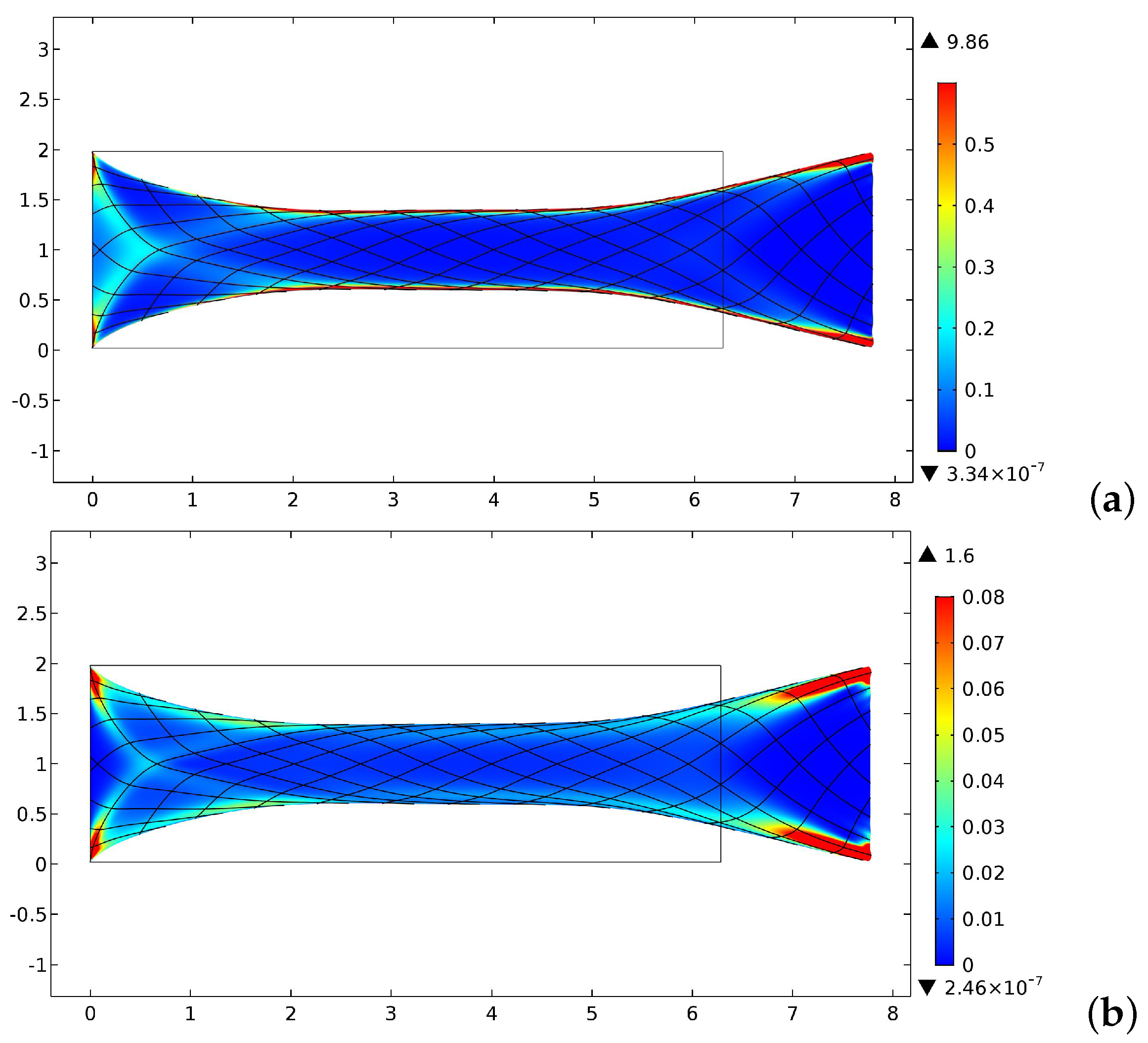
In the bias extension case, the cycloidal pantographic sheet was clamped to the left short end, and a displacement parallel to the longitudinal direction of the sample was prescribed on the opposite edge. In this first case, only Dirichlet conditions on displacement were considered. Therefore, we applied no double forces or couples. Figure 2 reports the equilibrium shape for an imposed displacement of 1.5 and being zero on the same edge. The lack of symmetry of the cycloidal lattice with respect to a vertical central axis reflects in the equilibrium shape, which exhibits the same feature. In addition to the distribution of the energy densities and , the figure shows also some material lines in the current configuration which initially lay along cycloids as in Figure 1.
In Figure 2, it is possible to see that both the energy densities are concentrated in a narrow layer at the long edges, as is expected, given the greater density of the fibers in that region and the more compliant disposition of those in the center.
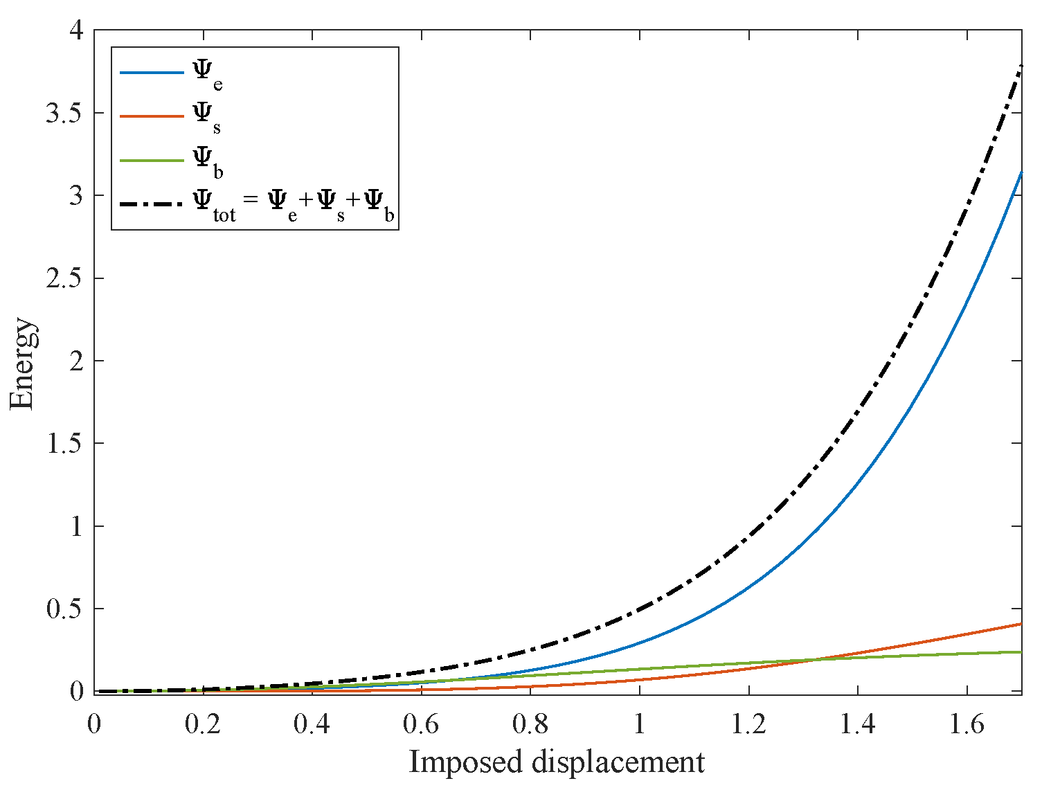
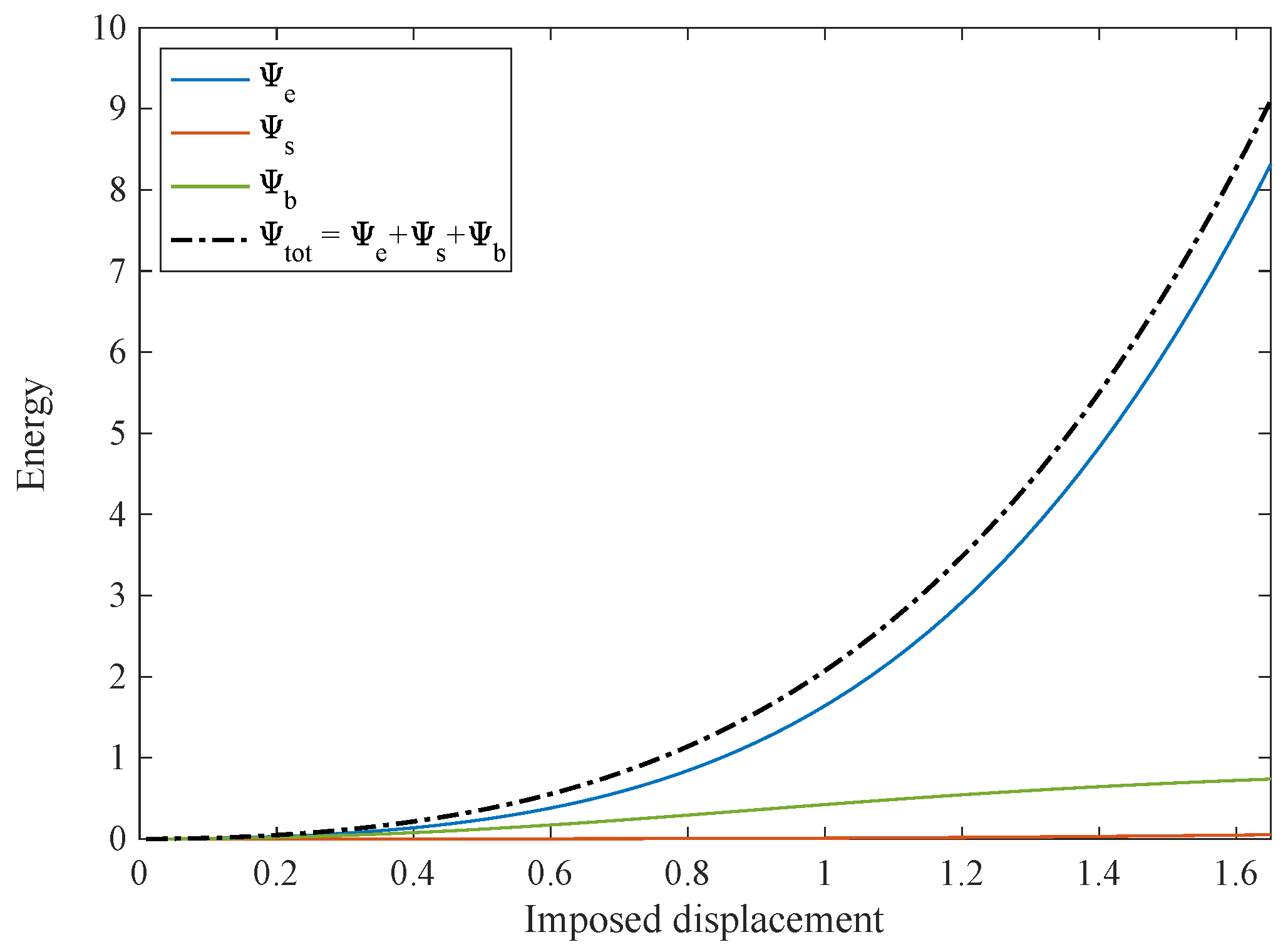
Figure 3 shows the contributions of the elastic energy versus the imposed displacement. We split the energy due to the first gradient in a piece accounting for the elongation of the fibers, namely the integral over the domain of the first two terms of Equation (26), , and in a piece due to the shear deformation, i.e., the integral of the last term of Equation (26), . Moreover, the part related to the second gradient responsible for the geodesic bending in this in-plane motion is also reported, i.e., , as well as the total energy stored in the deformation . The most significant contribution is related to fiber elongation.
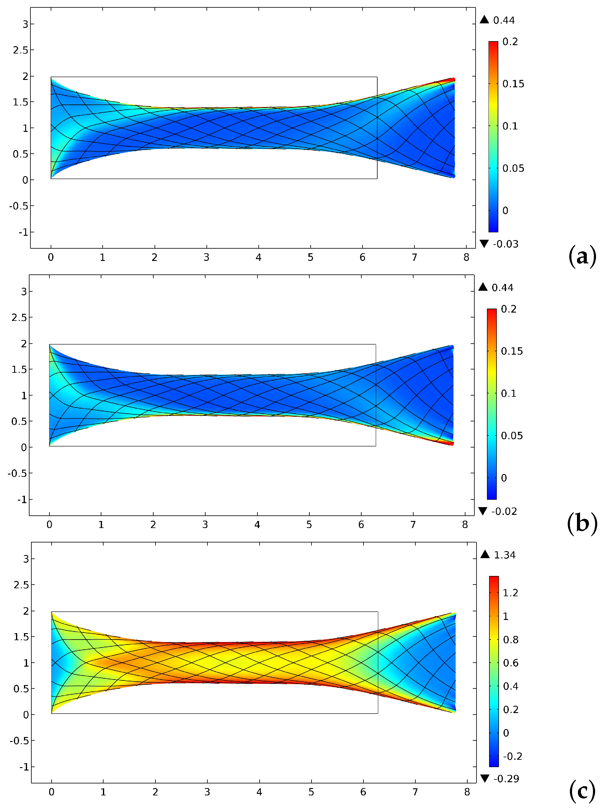
Similarly, the accumulation of the deformation along the most extended edges is visible also in Figure 4 that reports the distribution of the first gradient measures of deformation, namely , , and . The shear distortion is an exception because, for a certain amount, it is also spread in the central region.
3.2. Bias Compression Test
In a compression test, the analyzed surface with embedded fibers shows a buckling behavior. In detail, we considered a zero displacement on the short left side as in the previous case, while the imposed displacement in the opposite edge decreased until reached the value of −2. Besides, here, we also added the boundary conditions related to the normal derivative of the out-of-plane displacement, which was set to be zero on both the short edges, i.e., = 0.
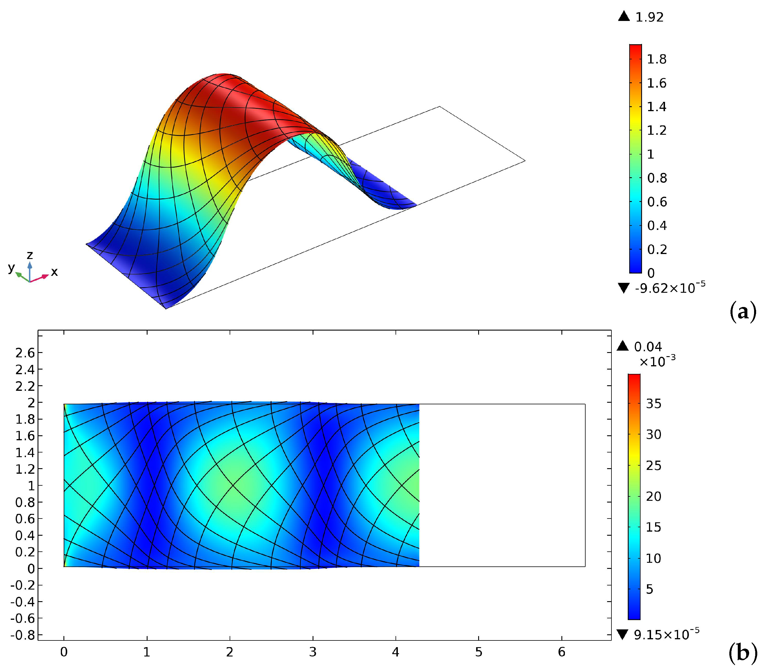
Figure 5 shows the buckled shape (Figure 5a) at the final imposed displacement. Figure 5b exhibits the second gradient contribution of the energy density since it is the most appreciable in such a case. It is also emphasized that here a lack of symmetry is perceivable if we observe the energy distribution and the material lines in the current configuration.
3.3. Shear Test
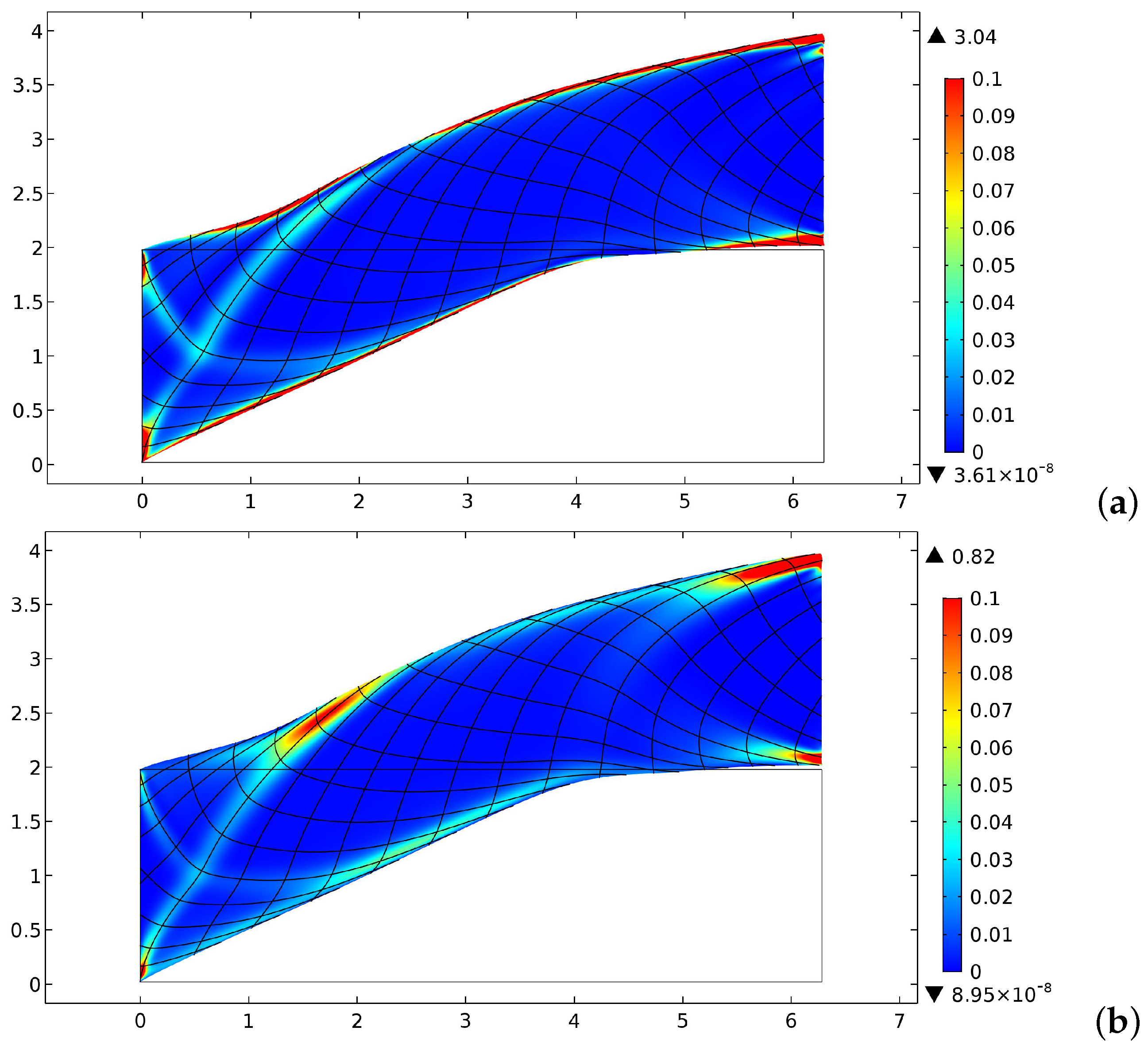
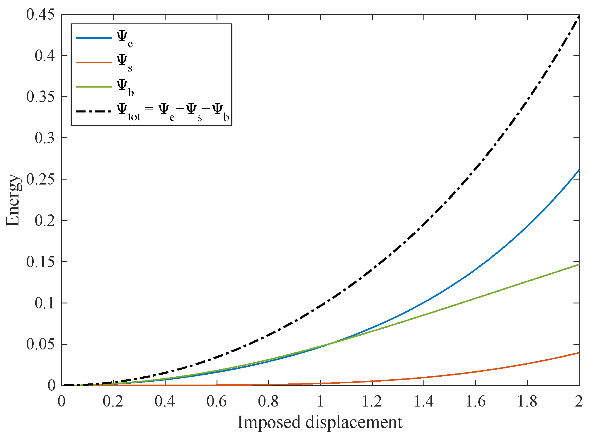
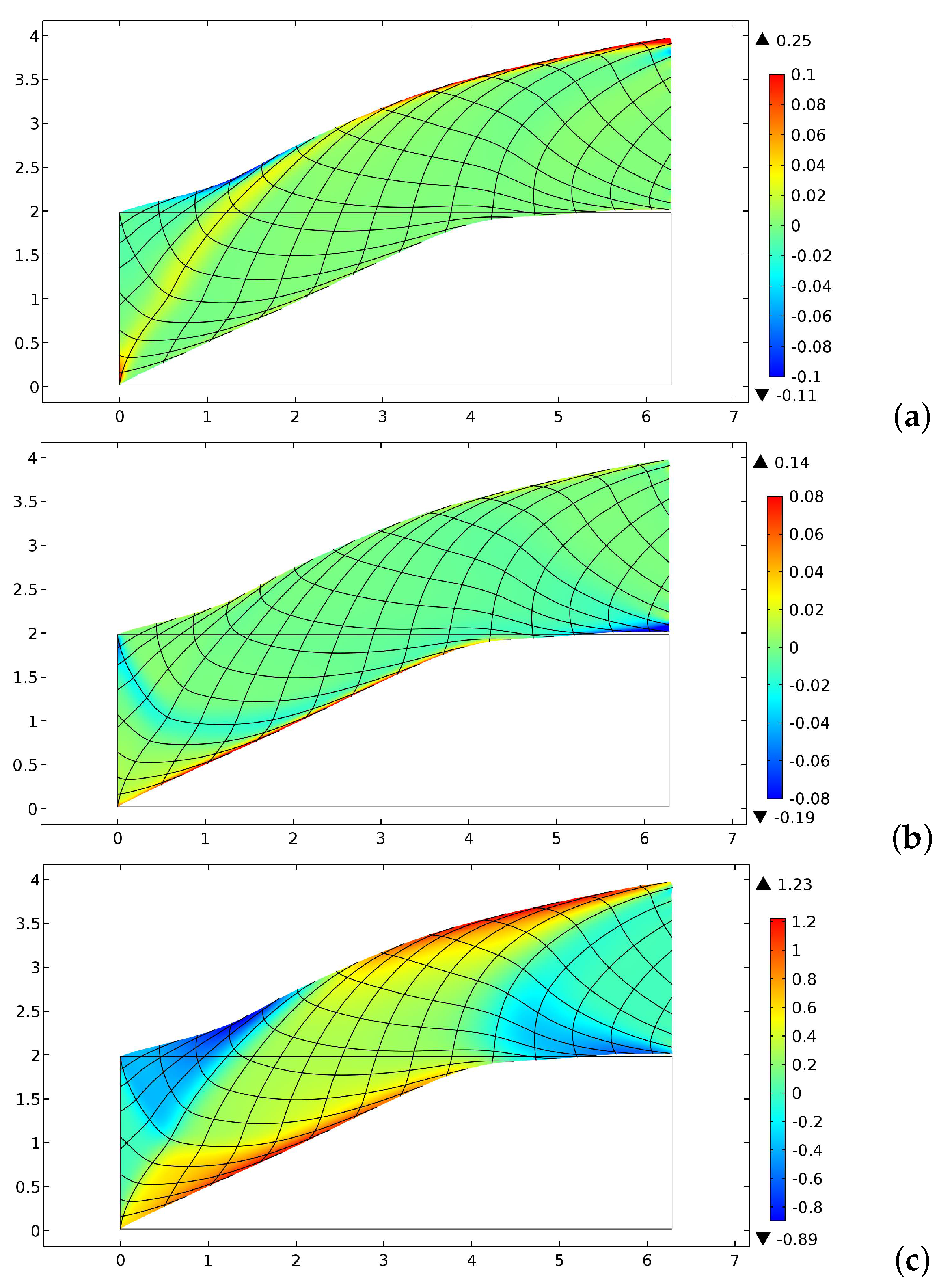
The equilibrium shape obtained in a shear test is presented in Figure 6. In this case, we considered the same boundary conditions of the bias test but the displacement imposed on the right short side was now equal to 2 while was fixed to zero on the same edge. In addition, in this case, both the energy density of the first and second gradient tend to be concentrated close to the long edges. The energy contributions depicted in Figure 7, differently from the bias extension test, show that the stretching and the geodesic bending energies are almost the same until the displacement equals 1.2. Similar considerations can be done in this case as for the bias extension test, for the first gradient measures of deformation, as can be detected by Figure 8.
3.4. Torsion Test
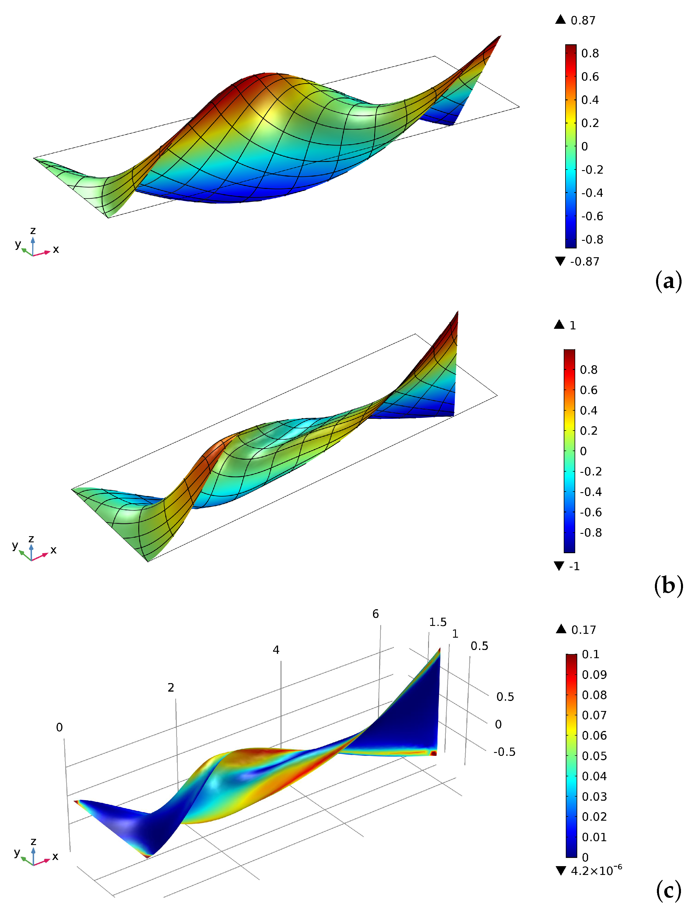
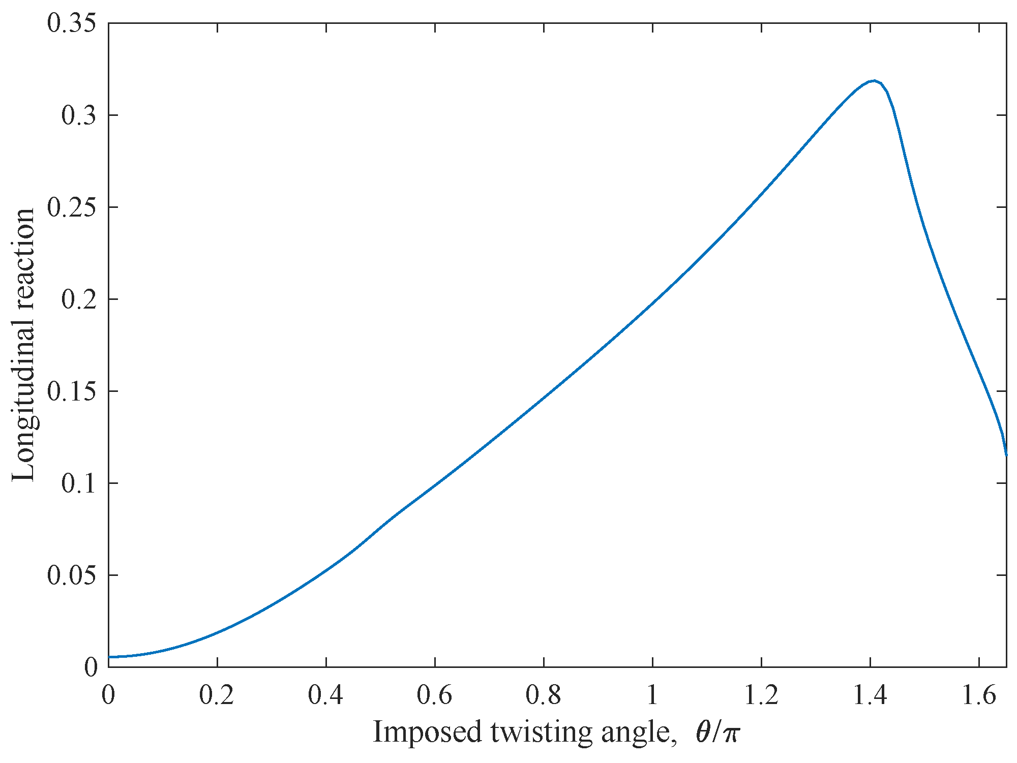
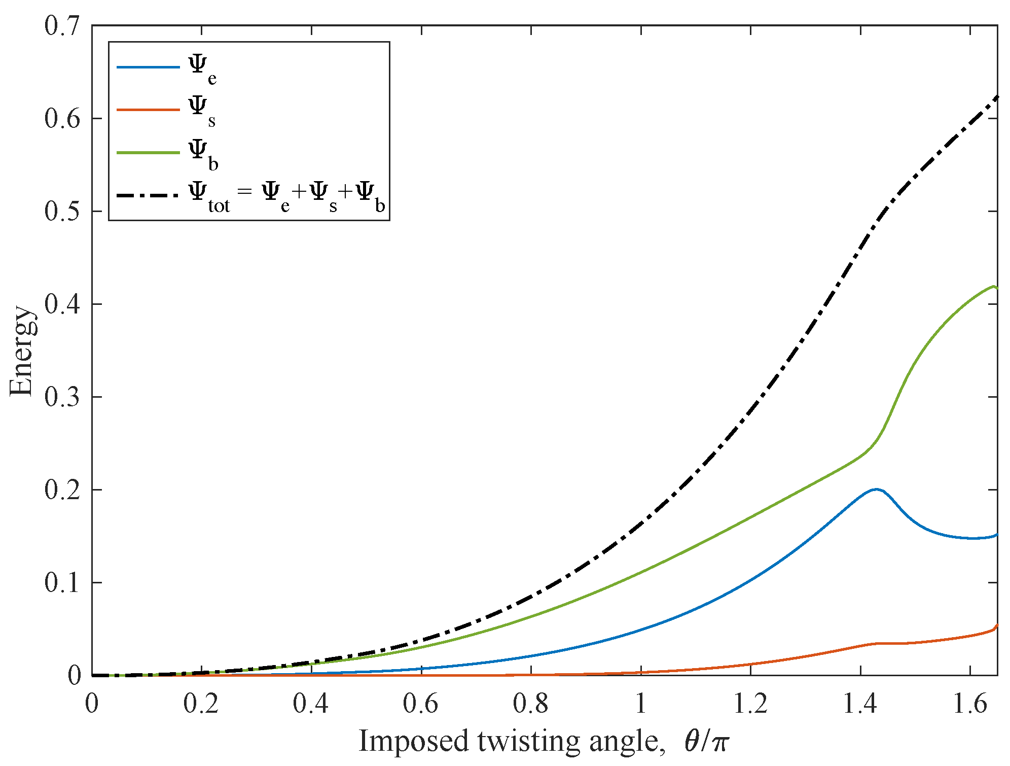
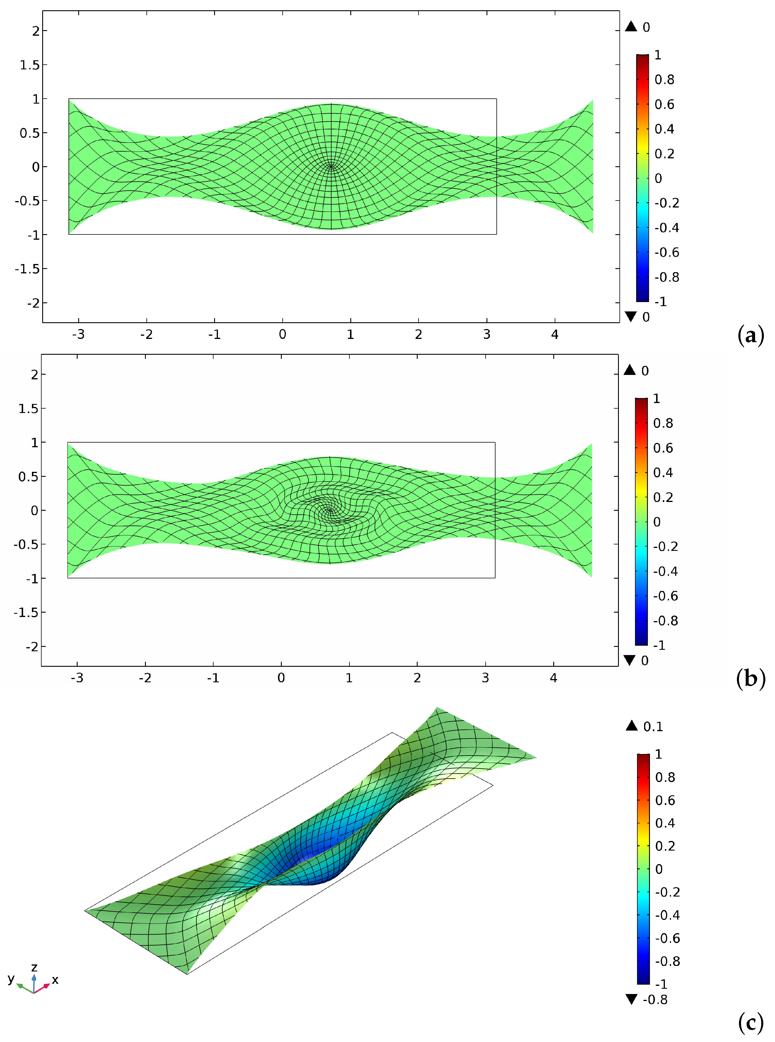
The last example is a torsion test where the displacements on the left short side were fixed, while the displacements of the short right side were evaluated to obtain a rigid rotation of an angle with respect to the central longitudinal axis of the sample. Moreover, the derivative with respect to the coordinate of the out-of-plane displacement was also put to zero on the short sides. In Figure 9 are reported two equilibrium shapes for a torsion angle of about and in Figure 9a,b, respectively. The former shape resembles a helix, while the latter equilibrium configuration is a buckled one. Indeed, in Figure 9b, the deformed surface presents a particular folding near the long borders deviating from the helix-type shape. Figure 9c shows with the colors the distribution of the second gradient energy density for the buckled shape. The presence of the buckling is evident if we see the plot of the longitudinal reaction on the short left side versus the torsion angle in Figure 10. After an angle of , a drop in the reaction due to the buckling behavior is quite evident. The presence of the buckling is also detectable looking at the energy contributions varying the rotation angle , as indicated by the diagrams in Figure 11, in correspondence of the suddenly change of the slope of the energy plots. Moreover, we observe that, after the occurrence of the buckling, the flexural/twisting energy increases notably while the extension energy decreases. This fact is conforming to the above-mentioned folding at the sides.
4. Comparison among the Pantographic Sheets with Orthogonal Lattices
In this section, we compare the results obtained for the cycloidal lattice with those related to linear and curvilinear lattices, especially for parabolic [55] and oscillatory ones [65]. The bias extension test described in Section 3.1 was numerically performed for all the cases in the same conditions adopted for the cycloidal sample, namely the size of the domain, the material parameters, and the boundary conditions.
In Figure 12, we plot the particular arrangement of fibers conceived for the parabolic pantographic sheet in the considered domain. Figure 13 shows the main characteristics of this pattern of fibers resulting from the bias extension test. In detail, due to the straight transversal fibers at the center of the specimen, the sample may experience a buckling in an extension test [86]. In such a test, the central transversal fibers are subjected to a significant compression indeed. Figure 13b,c displays the buckled shapes for different initial imperfection. If the deformation remains in the plane of the sample, we have a geodesic buckling, as reported in Figure 13b; otherwise, the buckled configuration assumes a typical spoon-shaped form (see Figure 13c and [87] for experimental evidence). Figure 13a shows the equilibrium configuration without any buckling.
According to Giorgio et al. [65], the oscillatory network of fibers is described by the two families of curves, as represented below in Cartesian coordinates:
where the amplitude A and the frequency of oscillation determine the behavior of the pantographic surface; in fact, the value of defines the number and the position of the regions in which the fibers tend to be denser, as shown in Figure 14, where a transverse accumulation of the fibers is evident. Of course, and select the specific curve of each family. In this case, the distribution of the fibers therefore entails a sort of transverse stiffeners which can be properly designed by choosing the values of A and . In what follows, we set and ;
Figure 15 shows the different contributions of the elastic energy versus the imposed displacement in the bias extension test. The oscillatory pantographic sheet is stiffer than the cycloidal one: for the same displacement imposed, it stores twice as much deformation energy. Moreover, the shear energy is almost negligible.
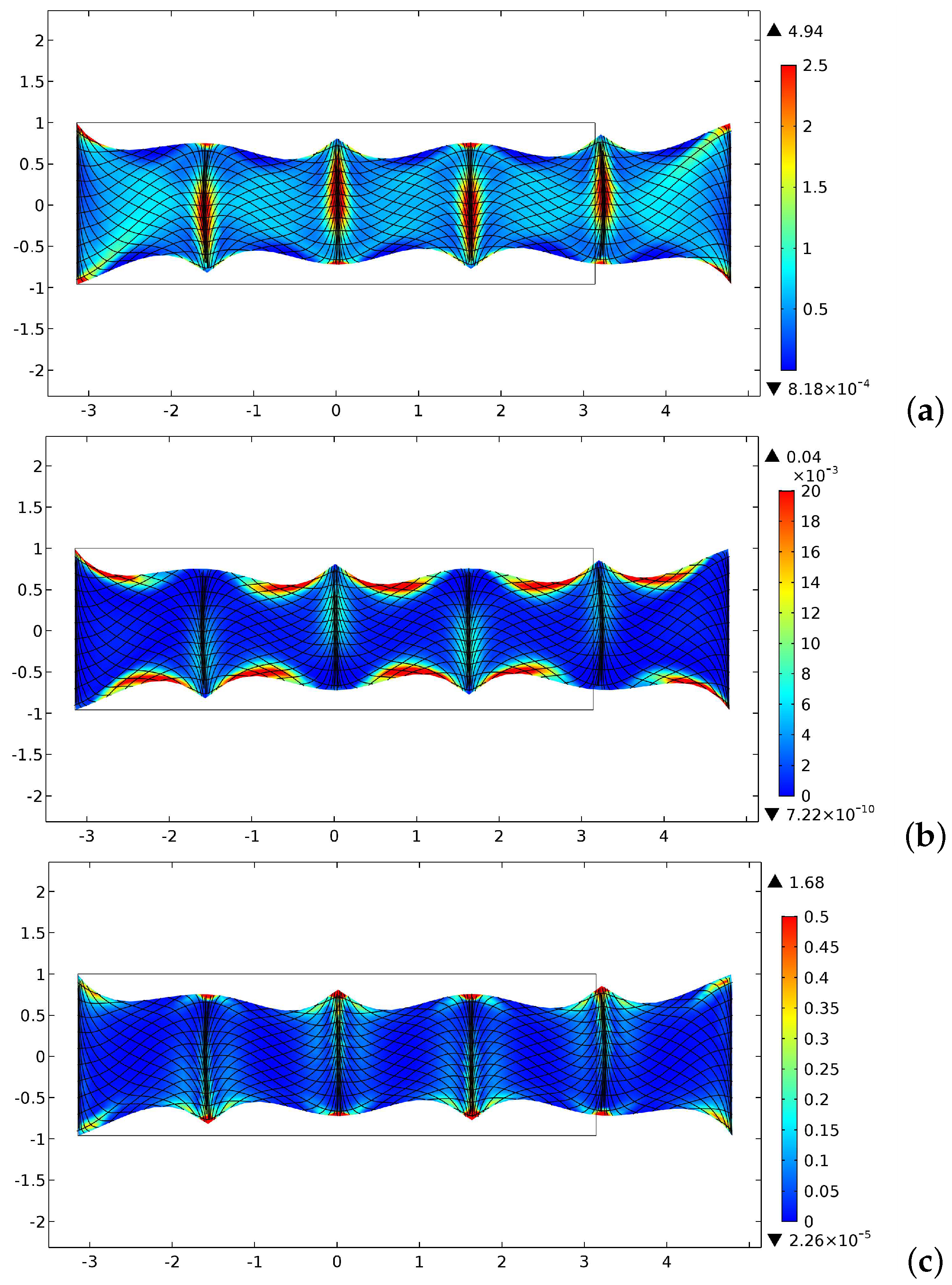
Figure 16 displays by colors, for an imposed displacement , the distributions of energy density related to the stretching (Figure 16a), the shear (Figure 16b), and the second gradient energy contribution (Figure 16c). Figure 16 also shows the equilibrium configuration in the considered test. As it is expected, in correspondence of the “stiffeners” due to the pattern of the fibers, the transverse deformation of the sample is less pronounced.
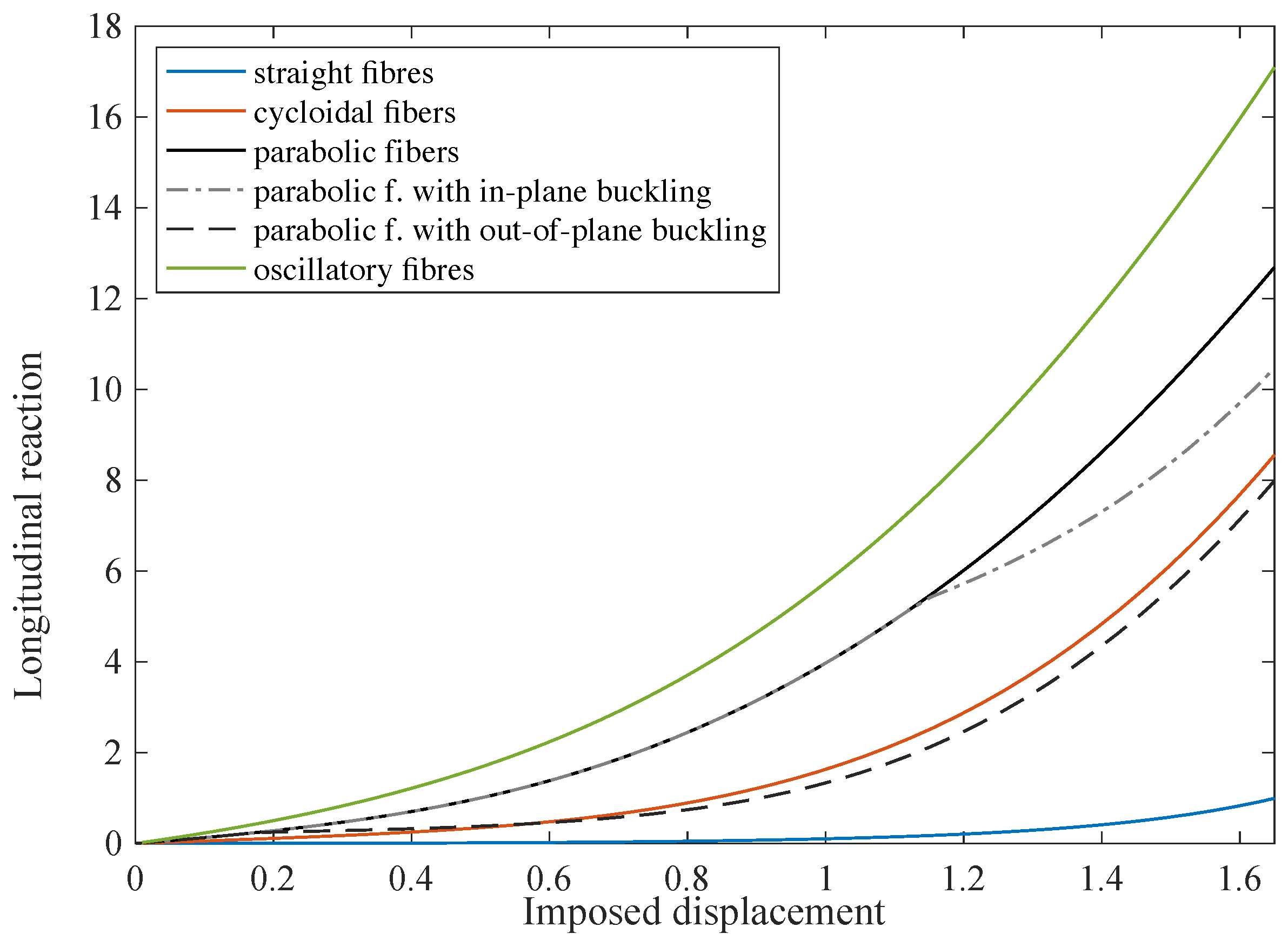
Finally, all the longitudinal reactions related to the different kinds of fiber arrangement are plotted in Figure 17 as a function of the imposed displacement for the sake of comparison. In the case of parabolic fibers, not only is the case without buckling plotted but also the two diagrams of the two detected bucklings are shown. From them, it is clear that the out-of-plane buckling is the most advantageous from an energetic point of view; this is the reason for which it is easily obtainable by experiments. The sample with straight fibers is the most compliant because of the pantographic effect, which is dominant. On the other hand, the oscillatory lattice corresponds to the stiffest one because of the multiple extra rigid regions of the pattern.
The cycloidal lattice has an intermediate behavior due to the simultaneous presence of a pantographic effect in the central zone and the particular orientation of the fibers along the more extended edges. Indeed, this particular fiber arrangement contributes to the longitudinal strength of the sample. We further remark that the cycloidal network has a load-bearing capacity almost similar to the parabolic lattice in the case of a spoon-shaped buckling. The case of a parabolic lattice without buckling is a metastable configuration. Thus, it is not attractive in many applications. A little more enticing may be the parabolic net with in-plane buckling in those cases in which there are extra constraints that compel the deformed configuration to remain plain.
Author Contributions
Conceptualization, D.S. and I.G.; methodology, D.S. and I.G.; formal analysis, D.S. and I.G.; investigation, D.S. and I.G.; writing—original draft preparation, D.S.; writing—review and editing, I.G.; and supervision, I.G.
Acknowledgments
The authors thank David J. Steigmann, Nicola L. Rizzi, and Francesco dell’Isola for helpful comments and advice through the study.
Conflicts of Interest
The authors declare no conflict of interest.
References
- El Sherbiny, M.G.; Placidi, L. Discrete and continuous aspects of some metamaterial elastic structures with band gaps. Arch. Appl. Mech. 2018, 88, 1725–1742. [Google Scholar] [CrossRef]
- Nejadsadeghi, N.; Placidi, L.; Romeo, M.; Misra, A. Frequency band gaps in dielectric granular metamaterials modulated by electric field. Mech. Res. Commun. 2019, 95, 96–103. [Google Scholar] [CrossRef]
- Vangelatos, Z.; Komvopoulos, K.; Grigoropoulos, C.P. Vacancies for controlling the behavior of microstructured three-dimensional mechanical metamaterials. Math. Mech. Solids 2019, 24, 511–524. [Google Scholar] [CrossRef]
- Laudato, M.; De Angelo, M. Workshop on Encounter of the third kind on Generalized continua and microstructures in Arpino, 3–7 April 2018: A review of presentations and discussions. Math. Mech. Solids 2019, 25, 117–126. [Google Scholar] [CrossRef]
- Barchiesi, E.; Spagnuolo, M.; Placidi, L. Mechanical metamaterials: A state of the art. Math. Mech. Solids 2019, 24, 212–234. [Google Scholar] [CrossRef]
- Yildizdag, M.E.; Tran, C.A.; Barchiesi, E.; Spagnuolo, M.; dell’Isola, F.; Hild, F. A Multi-disciplinary Approach for Mechanical Metamaterial Synthesis: A Hierarchical Modular Multiscale Cellular Structure Paradigm. In State of the Art and Future Trends in Material Modeling; Advanced Structured Materials; Altenbach, H.O.A., Ed.; Springer: Cham, Switzerland, 2019; Volume 100, pp. 485–505. [Google Scholar]
- Milton, G.; Briane, M.; Harutyunyan, D. On the possible effective elasticity tensors of 2-dimensional and 3-dimensional printed materials. Math. Mech. Complex Syst. 2017, 5, 41–94. [Google Scholar] [CrossRef] [Green Version]
- Placidi, L.; Barchiesi, E.; Turco, E.; Rizzi, N.L. A review on 2D models for the description of pantographic fabrics. Z. Angew. Math. Phys. 2016, 67, 121. [Google Scholar] [CrossRef]
- Barchiesi, E.; Placidi, L. A review on models for the 3D statics and 2D dynamics of pantographic fabrics. In Wave Dynamics and Composite Mechanics for Microstructured Materials and Metamaterials; Advanced Structured Materials; Sumbatyan, M., Ed.; Springer: Singapore, 2017; Volume 59, pp. 239–258. [Google Scholar]
- Cuomo, M.; dell’Isola, F.; Greco, L.; Rizzi, N.L. First versus second gradient energies for planar sheets with two families of inextensible fibres: Investigation on deformation boundary layers, discontinuities and geometrical instabilities. Compos. Part Eng. 2017, 115, 423–448. [Google Scholar] [CrossRef] [Green Version]
- De Angelo, M.; Spagnuolo, M.; D’Annibale, F.; Pfaff, A.; Hoschke, K.; Misra, A.; Dupuy, C.; Peyre, P.; Dirrenberger, J.; Pawlikowski, M. The macroscopic behavior of pantographic sheets depends mainly on their microstructure: Experimental evidence and qualitative analysis of damage in metallic specimens. Contin. Mech. Thermodyn. 2019, 31, 1181–1203. [Google Scholar] [CrossRef]
- Cuomo, M.; dell’Isola, F.; Greco, L. Simplified analysis of a generalized bias test for fabrics with two families of inextensible fibres. Z. Angew. Math. Phys. 2016, 67, 61. [Google Scholar] [CrossRef]
- Spagnuolo, M.; Barcz, K.; Pfaff, A.; dell’Isola, F.; Franciosi, P. Qualitative pivot damage analysis in aluminum printed pantographic sheets: Numerics and experiments. Mech. Res. Commun. 2017, 83, 47–52. [Google Scholar] [CrossRef] [Green Version]
- Barchiesi, E.; Ganzosch, G.; Liebold, C.; Placidi, L.; Grygoruk, R.; Müller, W.H. Out-of-plane buckling of pantographic fabrics in displacement-controlled shear tests: Experimental results and model validation. Contin. Mech. Thermodyn. 2019, 31, 33–45. [Google Scholar] [CrossRef]
- Turco, E.; Golaszewski, M.; Cazzani, A.; Rizzi, N.L. Large deformations induced in planar pantographic sheets by loads applied on fibers: Experimental validation of a discrete Lagrangian model. Mech. Res. Commun. 2016, 76, 51–56. [Google Scholar] [CrossRef]
- Alibert, J.J.; Seppecher, P.; dell’Isola, F. Truss modular beams with deformation energy depending on higher displacement gradients. Math. Mech. Solids 2003, 8, 51–73. [Google Scholar] [CrossRef]
- Dell’Isola, F.; Lekszycki, T.; Pawlikowski, M.; Grygoruk, R.; Greco, L. Designing a light fabric metamaterial being highly macroscopically tough under directional extension: First experimental evidence. Z. Angew. Math. Phys. 2015, 66, 3473–3498. [Google Scholar] [CrossRef]
- Dell’Isola, F.; Andreaus, U.; Placidi, L. At the origins and in the vanguard of peridynamics, non-local and higher-gradient continuum mechanics: An underestimated and still topical contribution of Gabrio Piola. Math. Mech. Solids 2015, 20, 887–928. [Google Scholar] [CrossRef]
- Franciosi, P.; Spagnuolo, M.; Salman, O.U. Mean Green operators of deformable fiber networks embedded in a compliant matrix and property estimates. Contin. Mech. Thermodyn. 2019, 31, 101–132. [Google Scholar] [CrossRef]
- Spagnuolo, M.; Franciosi, P.; dell’Isola, F. A Green operator-based elastic modeling for two-phase pantographic-inspired bi-continuous materials. Int. J. Solids Struct. 2019. [Google Scholar] [CrossRef]
- Avella, M.; Casale, L.; Dell’Erba, R.; Martuscelli, E. Broom fibers as reinforcement for thermoplastic matrices. In Macromolecular Symposia; Hüthig & Wepf Verlag: Basel, Switzerland, 1998. [Google Scholar]
- Avella, M.; Dell’Erba, R.; Martuscelli, E. Fiber reinforced polypropylene: Influence of iPP molecular weight on morphology, crystallization, and thermal and mechanical properties. Polym. Compos. 1996, 17, 288–299. [Google Scholar] [CrossRef]
- Haseganu, E.M.; Steigmann, D.J. Equilibrium analysis of finitely deformed elastic networks. Comput. Mech. 1996, 17, 359–373. [Google Scholar] [CrossRef]
- Atai, A.A.; Steigmann, D.J. On the nonlinear mechanics of discrete networks. Arch. Appl. Mech. 1997, 67, 303–319. [Google Scholar] [CrossRef]
- Steigmann, D.J. Continuum theory for elastic sheets formed by inextensible crossed elasticae. Int. J. Non-Linear Mech. 2018, 106, 324–329. [Google Scholar] [CrossRef]
- Eugster, S.; dell’Isola, F.; Steigmann, D.J. Continuum theory for mechanical metamaterials with a cubic lattice substructure. Math. Mech. Complex Syst. 2019, 7, 75–98. [Google Scholar] [CrossRef] [Green Version]
- Eremeyev, V.A. Two-and three-dimensional elastic networks with rigid junctions: Modeling within the theory of micropolar shells and solids. Acta Mech. 2019, 230, 3875–3887. [Google Scholar] [CrossRef] [Green Version]
- Eremeyev, V.A. A Nonlinear Model of a Mesh Shell. Mech. Solids 2018, 53, 464–469. [Google Scholar] [CrossRef]
- Boutin, C.; Hans, S.; Chesnais, C. Generalized beams and continua. Dynamics of reticulated structures. In Mechanics of Generalized Continua; Advances in Mechanics and Mathematics; Maugin, G., Metrikine, A., Eds.; Springer: New York, NY, USA, 2010; Volume 21, pp. 131–141. [Google Scholar]
- Pideri, C.; Seppecher, P. A second gradient material resulting from the homogenization of an heterogeneous linear elastic medium. Contin. Mech. Thermodyn. 1997, 9, 241–257. [Google Scholar] [CrossRef] [Green Version]
- Abdoul-Anziz, H.; Seppecher, P.; Bellis, C. Homogenization of frame lattices leading to second gradient models coupling classical strain and strain-gradient terms. Math. Mech. Solids 2019, 24, 3976–3999. [Google Scholar] [CrossRef] [Green Version]
- Abdoul-Anziz, H.; Seppecher, P. Strain gradient and generalized continua obtained by homogenizing frame lattices. Math. Mech. Complex Syst. 2018, 6, 213–250. [Google Scholar] [CrossRef] [Green Version]
- Berrehili, Y.; Marigo, J.J. The homogenized behavior of unidirectional fiber-reinforced composite materials in the case of debonded fibers. Math. Mech. Complex Syst. 2014, 2, 181–207. [Google Scholar] [CrossRef] [Green Version]
- Placidi, L.; dell’Isola, F.; Barchiesi, E. Heuristic Homogenization of Euler and Pantographic Beams. In Mechanics of Fibrous Materials and Applications; CISM International Centre for Mechanical Sciences (Courses and Lectures); Picu, C., Ganghoffer, J.F., Eds.; Springer: Cham, Switzerland, 2020; Volume 596, pp. 123–155. [Google Scholar]
- Dos Reis, F.; Ganghoffer, J.F. Equivalent mechanical properties of auxetic lattices from discrete homogenization. Comput. Mater. Sci. 2012, 51, 314–321. [Google Scholar] [CrossRef]
- Dos Reis, F.; Ganghoffer, J.F. Construction of micropolar continua from the asymptotic homogenization of beam lattices. Comput. Struct. 2012, 112, 354–363. [Google Scholar] [CrossRef]
- Eremeyev, V.A.; Pietraszkiewicz, W. Material symmetry group and constitutive equations of micropolar anisotropic elastic solids. Math. Mech. Solids 2016, 21, 210–221. [Google Scholar] [CrossRef]
- Eremeyev, V.A.; Pietraszkiewicz, W. Material symmetry group of the non-linear polar-elastic continuum. Int. J. Solids Struct. 2012, 49, 1993–2005. [Google Scholar] [CrossRef] [Green Version]
- Altenbach, H.; Eremeyev, V. On the constitutive equations of viscoelastic micropolar plates and shells of differential type. Math. Mech. Complex Syst. 2015, 3, 273–283. [Google Scholar] [CrossRef]
- Battista, A.; Cardillo, C.; Del Vescovo, D.; Rizzi, N.L.; Turco, E. Frequency shifts induced by large deformations in planar pantographic continua. Nanosci. Technol. Int. J. 2015, 6, 161–178. [Google Scholar] [CrossRef]
- Laudato, M.; Barchiesi, E. Non-linear Dynamics of Pantographic Fabrics: Modelling and Numerical Study. In Wave Dynamics, Mechanics and Physics of Microstructured Metamaterials; Advanced Structured Materials; Sumbatyan, M., Ed.; Springer: Cham, Switzerland, 2019; Volume 109, pp. 241–254. [Google Scholar]
- Eremeyev, V.A.; Sharma, B.L. Anti-plane surface waves in media with surface structure: Discrete vs. continuum model. Int. J. Eng. Sci. 2019, 143, 33–38. [Google Scholar] [CrossRef] [Green Version]
- Scala, I.; Rosi, G.; Placidi, L.; Nguyen, V.H.; Naili, S. Effects of the microstructure and density profiles on wave propagation across an interface with material properties. Contin. Mech. Thermodyn. 2019, 31, 1165–1180. [Google Scholar] [CrossRef]
- Engelbrecht, J.; Berezovski, A. Reflections on mathematical models of deformation waves in elastic microstructured solids. Math. Mech. Complex Syst. 2015, 3, 43–82. [Google Scholar] [CrossRef]
- Eremeyev, V.A. Strongly anisotropic surface elasticity and antiplane surface waves. Philos. Trans. R. Soc. 2019, 378, 1–14. [Google Scholar] [CrossRef] [Green Version]
- Moretti, P.F.; Grzybowski, B.A.; Basios, V.; Fortunato, E.; Diez, M.S.; Speck, O.; Martins, R. STEM materials: A new frontier for an intelligent sustainable world. BMC Mater. 2019, 1, 1–3. [Google Scholar] [CrossRef] [Green Version]
- Altenbach, H.; Eremeyev, V.A. Direct approach-based analysis of plates composed of functionally graded materials. Arch. Appl. Mech. 2008, 78, 775–794. [Google Scholar] [CrossRef] [Green Version]
- Seppecher, P.; Alibert, J.J.; dell’Isola, F. Linear elastic trusses leading to continua with exotic mechanical interactions. J. Phys. 2011, 319, 012018. [Google Scholar] [CrossRef]
- Dell’Isola, F.; Turco, E.; Misra, A.; Vangelatos, Z.; Grigoropoulos, C.; Melissinaki, V.; Farsari, M. Force–displacement relationship in micro-metric pantographs: Experiments and numerical simulations. Comptes Rendus Mec. 2019, 347, 397–405. [Google Scholar] [CrossRef]
- Nejadsadeghi, N.; De Angelo, M.; Drobnicki, R.; Lekszycki, T.; dell’Isola, F.; Misra, A. Parametric Experimentation on Pantographic Unit Cells Reveals Local Extremum Configuration. Exp. Mech. 2019, 59, 927–939. [Google Scholar] [CrossRef] [Green Version]
- Barchiesi, E.; Eugster, S.R.; Placidi, L.; dell’Isola, F. Pantographic beam: A complete second gradient 1D-continuum in plane. Z. Angew. Math. Phys. Angew. Math. Phys. 2019, 70, 135. [Google Scholar] [CrossRef] [Green Version]
- Dell’Isola, F.; Steigmann, D. A two-dimensional gradient-elasticity theory for woven fabrics. J. Elast. 2015, 118, 113–125. [Google Scholar] [CrossRef] [Green Version]
- Steigmann, D.J.; dell’Isola, F. Mechanical response of fabric sheets to three-dimensional bending, twisting, and stretching. Acta Mech. Sin. 2015, 31, 373–382. [Google Scholar] [CrossRef]
- Steigmann, D.J.; Pipkin, A.C. Equilibrium of elastic nets. Philos. Trans. R. Soc. London. Ser. Phys. Eng. Sci. 1991, 335, 419–454. [Google Scholar]
- Scerrato, D.; Giorgio, I.; Rizzi, N.L. Three-dimensional instabilities of pantographic sheets with parabolic lattices: Numerical investigations. Z. Angew. Math. Phys. 2016, 67, 53. [Google Scholar] [CrossRef] [Green Version]
- Placidi, L.; Barchiesi, E.; Della Corte, A. Identification of two-dimensional pantographic structures with a linear D4 orthotropic second gradient elastic model accounting for external bulk double forces. In Mathematical Modelling in Solid Mechanics; Advanced Structured Materials; dell’Isola, F., Sofonea, M., Steigmann, D., Eds.; Springer: Singapore, 2017; Volume 69, pp. 211–232. [Google Scholar]
- Harrison, P. Modelling the forming mechanics of engineering fabrics using a mutually constrained pantographic beam and membrane mesh. Compos. Part Appl. Sci. Manuf. 2016, 81, 145–157. [Google Scholar] [CrossRef] [Green Version]
- Harrison, P.; Alvarez, M.F.; Anderson, D. Towards comprehensive characterisation and modelling of the forming and wrinkling mechanics of engineering fabrics. Int. J. Solids Struct. 2018, 154, 2–18. [Google Scholar] [CrossRef] [Green Version]
- Rosi, G.; Placidi, L.; Auffray, N. On the validity range of strain-gradient elasticity: A mixed static-dynamic identification procedure. Eur. J. Mech. A Solids 2018, 69, 179–191. [Google Scholar] [CrossRef] [Green Version]
- Abali, B.E.; Wu, C.C.; Müller, W.H. An energy-based method to determine material constants in nonlinear rheology with applications. Contin. Mech. Thermodyn. 2016, 28, 1221–1246. [Google Scholar] [CrossRef]
- Abali, B.E.; Müller, W.H.; Eremeyev, V.A. Strain gradient elasticity with geometric nonlinearities and its computational evaluation. Mech. Adv. Mater. Mod. Process. 2015, 1, 4. [Google Scholar] [CrossRef] [Green Version]
- Misra, A.; Poorsolhjouy, P. Identification of higher-order elastic constants for grain assemblies based upon granular micromechanics. Math. Mech. Complex Syst. 2015, 3, 285–308. [Google Scholar] [CrossRef] [Green Version]
- Argyris, J.H.; Fried, I.; Scharpf, D.W. The TUBA family of plate elements for the matrix displacement method. Aeronaut. J. 1968, 72, 701–709. [Google Scholar] [CrossRef]
- Gustafsson, T.; Stenberg, R.; Videman, J. A posteriori estimates for conforming Kirchhoff plate elements. SIAM J. Sci. Comput. 2018, 40, A1386–A1407. [Google Scholar] [CrossRef] [Green Version]
- Giorgio, I.; Della Corte, A.; dell’Isola, F.; Steigmann, D.J. Buckling modes in pantographic lattices. Comptes Rendus Mec. 2016, 344, 487–501. [Google Scholar] [CrossRef]
- Wang, C.M.; Zhang, H.; Gao, R.P.; Duan, W.H.; Challamel, N. Hencky bar-chain model for buckling and vibration of beams with elastic end restraints. Int. J. Struct. Stab. Dyn. 2015, 15, 1540007. [Google Scholar] [CrossRef]
- Turco, E. Discrete is it enough? The revival of Piola–Hencky keynotes to analyze three-dimensional Elastica. Contin. Mech. Thermodyn. 2018, 30, 1039–1057. [Google Scholar] [CrossRef]
- Turco, E.; dell’Isola, F.; Cazzani, A.; Rizzi, N.L. Hencky-type discrete model for pantographic structures: Numerical comparison with second gradient continuum models. Z. Angew. Math. Phys. 2016, 67, 85. [Google Scholar] [CrossRef] [Green Version]
- Turco, E.; Misra, A.; Pawlikowski, M.; dell’Isola, F.; Hild, F. Enhanced Piola–Hencky discrete models for pantographic sheets with pivots without deformation energy: Numerics and experiments. Int. J. Solids Struct. 2018, 147, 94–109. [Google Scholar] [CrossRef] [Green Version]
- Andreaus, U.; Spagnuolo, M.; Lekszycki, T.; Eugster, S.R. A Ritz approach for the static analysis of planar pantographic structures modeled with nonlinear Euler–Bernoulli beams. Contin. Mech. Thermodyn. 2018, 30, 1103–1123. [Google Scholar] [CrossRef]
- Greco, L.; Cuomo, M.; Contrafatto, L. Two new triangular G1-conforming finite elements with cubic edge rotation for the analysis of Kirchhoff plates. Comput. Methods Appl. Mech. Eng. 2019, 356, 354–386. [Google Scholar] [CrossRef]
- Greco, L.; Cuomo, M.; Contrafatto, L. A quadrilateral G1-conforming finite element for the Kirchhoff plate model. Comput. Methods Appl. Mech. Eng. 2019, 346, 913–951. [Google Scholar] [CrossRef]
- Cuomo, M.; Greco, L. An implicit strong G1-conforming formulation for the analysis of the Kirchhoff plate model. Contin. Mech. Thermodyn. 2018. [Google Scholar] [CrossRef]
- Greco, L.; Cuomo, M.; Contrafatto, L. A reconstructed local B formulation for isogeometric Kirchhoff–Love shells. Comput. Methods Appl. Mech. Eng. 2018, 332, 462–487. [Google Scholar] [CrossRef]
- Turco, E.; Caracciolo, P. Elasto-plastic analysis of Kirchhoff plates by high simplicity finite elements. Comput. Methods Appl. Mech. Eng. 2000, 190, 691–706. [Google Scholar] [CrossRef]
- Niiranen, J.; Kiendl, J.; Niemi, A.H.; Reali, A. Isogeometric analysis for sixth-order boundary value problems of gradient-elastic Kirchhoff plates. Comput. Methods Appl. Mech. Eng. 2017, 316, 328–348. [Google Scholar] [CrossRef]
- Cazzani, A.; Malagù, M.; Turco, E.; Stochino, F. Constitutive models for strongly curved beams in the frame of isogeometric analysis. Math. Mech. Solids 2016, 21, 182–209. [Google Scholar] [CrossRef]
- Cazzani, A.; Malagù, M.; Turco, E. Isogeometric analysis of plane-curved beams. Math. Mech. Solids 2016, 21, 562–577. [Google Scholar] [CrossRef]
- Niiranen, J.; Balobanov, V.; Kiendl, J.; Hosseini, S.B. Variational formulations, model comparisons and numerical methods for Euler–Bernoulli micro-and nano-beam models. Math. Mech. Solids 2019, 24, 312–335. [Google Scholar] [CrossRef] [Green Version]
- Balobanov, V.; Niiranen, J. Locking-free variational formulations and isogeometric analysis for the Timoshenko beam models of strain gradient and classical elasticity. Comput. Methods Appl. Mech. Eng. 2018, 339, 137–159. [Google Scholar] [CrossRef]
- Maurin, F.; Greco, F.; Desmet, W. Isogeometric analysis for nonlinear planar pantographic lattice: discrete and continuum models. Contin. Mech. Thermodyn. 2019, 31, 1051–1064. [Google Scholar] [CrossRef]
- Yildizdag, M.E.; Demirtas, M.; Ergin, A. Multipatch discontinuous Galerkin isogeometric analysis of composite laminates. Contin. Mech. Thermodyn. 2018. [Google Scholar] [CrossRef]
- Khakalo, S.; Balobanov, V.; Niiranen, J. Modelling size-dependent bending, buckling and vibrations of 2D triangular lattices by strain gradient elasticity models: Applications to sandwich beams and auxetics. Int. J. Eng. Sci. 2018, 127, 33–52. [Google Scholar] [CrossRef] [Green Version]
- Cazzani, A.; Serra, M.; Stochino, F.; Turco, E. A refined assumed strain finite element model for statics and dynamics of laminated plates. Contin. Mech. Thermodyn. 2018. [Google Scholar] [CrossRef]
- Cazzani, A.; Rizzi, N.L.; Stochino, F.; Turco, E. Modal analysis of laminates by a mixed assumed-strain finite element model. Math. Mech. Solids 2018, 23, 99–119. [Google Scholar] [CrossRef]
- Spagnuolo, M.; Andreaus, U. A targeted review on large deformations of planar elastic beams: Extensibility, distributed loads, buckling and post-buckling. Math. Mech. Solids 2019, 24, 258–280. [Google Scholar] [CrossRef]
- Dell’Isola, F.; Seppecher, P.; Alibert, J.J.; Lekszycki, T.; Grygoruk, R.; Pawlikowski, M.; Gołaszewski, M. Pantographic metamaterials: An example of mathematically driven design and of its technological challenges. Contin. Mech. Thermodyn. 2019, 31, 851–884. [Google Scholar] [CrossRef] [Green Version]
Figure 1.
Scheme of a cycloidal orthogonal network of fibers. Solid blue lines are the graphs of Equation (1), while solid red lines refer to Equation (2).

Figure 2.
Distribution of the strain–energy density for the bias extension test: (a) contribution; and (b) contribution.
Figure 2.
Distribution of the strain–energy density for the bias extension test: (a) contribution; and (b) contribution.

Figure 3.
Strain–energy contributions for the bias extension test: extensional energy, ; shear energy, ; bending energy, ; and total energy .
Figure 3.
Strain–energy contributions for the bias extension test: extensional energy, ; shear energy, ; bending energy, ; and total energy .

Figure 4.
Distribution of the deformation measures of first gradient for the bias extension test: (a) ; (b) ; and (c) .
Figure 4.
Distribution of the deformation measures of first gradient for the bias extension test: (a) ; (b) ; and (c) .

Figure 5.
Bias compression test: (a) buckled shape, colors indicate the out-of-plane displacement; and (b) second gradient energy contribution, .
Figure 5.
Bias compression test: (a) buckled shape, colors indicate the out-of-plane displacement; and (b) second gradient energy contribution, .

Figure 6.
Distribution of the strain–energy density for the shear test: (a) contribution; and (b) contribution.
Figure 6.
Distribution of the strain–energy density for the shear test: (a) contribution; and (b) contribution.

Figure 7.
Strain–energy contributions for the shear test: extensional energy, ; shear energy, ; bending energy, ; and total energy .
Figure 7.
Strain–energy contributions for the shear test: extensional energy, ; shear energy, ; bending energy, ; and total energy .

Figure 8.
Distribution of the deformation measures of first gradient for the shear test: (a) ; (b) ; and (c) .
Figure 8.
Distribution of the deformation measures of first gradient for the shear test: (a) ; (b) ; and (c) .

Figure 9.
Torsion test: (a) equilibrium shape without buckling, where colors indicate the out-of-plane displacement; (b) buckled shape, where colors indicate the out-of-plane displacement; and (c) buckled shape, where colors indicate the second gradient energy .
Figure 9.
Torsion test: (a) equilibrium shape without buckling, where colors indicate the out-of-plane displacement; (b) buckled shape, where colors indicate the out-of-plane displacement; and (c) buckled shape, where colors indicate the second gradient energy .

Figure 10.
Longitudinal reaction for the torsion test.

Figure 11.
Strain–energy contributions for the torsion test: extensional energy, ; shear energy, ; flexural/twisting energy, ; and total energy .
Figure 11.
Strain–energy contributions for the torsion test: extensional energy, ; shear energy, ; flexural/twisting energy, ; and total energy .

Figure 12.
Scheme of a parabolic orthogonal network of fibers.

Figure 13.
Bias extension test: (a) equilibrium shape without buckling (imposed displacement ); (b) in-plane buckled shape (); and (c) out-of-plane buckled shape ().
Figure 13.
Bias extension test: (a) equilibrium shape without buckling (imposed displacement ); (b) in-plane buckled shape (); and (c) out-of-plane buckled shape ().

Figure 14.
Scheme of an oscillatory orthogonal network of fibers. Solid blue lines are the graphs of Equation (32), while solid red lines refer to Equation (33).
Figure 14.
Scheme of an oscillatory orthogonal network of fibers. Solid blue lines are the graphs of Equation (32), while solid red lines refer to Equation (33).

Figure 15.
Strain–energy contributions for the bias extension test for sample with oscillatory fibers: extensional energy, ; shear energy, ; bending energy, ; and total energy .
Figure 15.
Strain–energy contributions for the bias extension test for sample with oscillatory fibers: extensional energy, ; shear energy, ; bending energy, ; and total energy .

Figure 16.
Distribution of the strain–energy density for the bias extension test for sample with oscillatory fibers: (a) stretching contribution; (b) shear contribution; and (c) contribution.
Figure 16.
Distribution of the strain–energy density for the bias extension test for sample with oscillatory fibers: (a) stretching contribution; (b) shear contribution; and (c) contribution.

Figure 17.
Longitudinal reaction for the bias extension test: comparison among different cases of fibers.
Figure 17.
Longitudinal reaction for the bias extension test: comparison among different cases of fibers.

© 2019 by the authors. Licensee MDPI, Basel, Switzerland. This article is an open access article distributed under the terms and conditions of the Creative Commons Attribution (CC BY) license (http://creativecommons.org/licenses/by/4.0/).
Share and Cite
MDPI and ACS Style
Scerrato, D.; Giorgio, I. Equilibrium of Two-Dimensional Cycloidal Pantographic Metamaterials in Three-Dimensional Deformations. Symmetry 2019, 11, 1523. https://0-doi-org.brum.beds.ac.uk/10.3390/sym11121523
AMA Style
Scerrato D, Giorgio I. Equilibrium of Two-Dimensional Cycloidal Pantographic Metamaterials in Three-Dimensional Deformations. Symmetry. 2019; 11(12):1523. https://0-doi-org.brum.beds.ac.uk/10.3390/sym11121523
Chicago/Turabian StyleScerrato, Daria, and Ivan Giorgio. 2019. "Equilibrium of Two-Dimensional Cycloidal Pantographic Metamaterials in Three-Dimensional Deformations" Symmetry 11, no. 12: 1523. https://0-doi-org.brum.beds.ac.uk/10.3390/sym11121523
Note that from the first issue of 2016, this journal uses article numbers instead of page numbers. See further details here.