On the Effect of Thomson and Initial Stress in a Thermo-Porous Elastic Solid under G-N Electromagnetic Theory


1
Zagazig Higher Institute of Engineering & Technology, Ministry of Higher Education, P.O. Box 44519, Zagazig, Egypt
2
Department of Mathematics and Computer Science, Transilvania University of Brasov, Brasov 500036, Romania
3
Department of Mathematics, Faculty of Science, Zagazig University, P.O. Box 44519, Zagazig, Egypt
*
Author to whom correspondence should be addressed.
Symmetry 2019, 11(3), 413; https://0-doi-org.brum.beds.ac.uk/10.3390/sym11030413
Submission received: 22 January 2019
/
Revised: 6 March 2019
/
Accepted: 14 March 2019
/
Published: 20 March 2019
(This article belongs to the Special Issue Symmetry in Applied Continuous Mechanics)
Abstract
:The present work investigated the effect of Thomson and initial stress in a thermo-porous elastic solid under G-N electromagnetic theory. The Thomson coefficient affects the heat condition equation. A constant Thomson coefficient, instead of traditionally a constant Seebeck coefficient, is assumed. The charge density of the induced electric current is taken as a function of time. A normal mode method is proposed to analyze the problem and to obtain numerical solutions. The results that were obtained for all physical sizes are graphically illustrated and we offer a comparison between the type II G-N theory and the G-N theory of type III, both in the present case and in the absence of specific parameters, as initial stress, pores and the Thomson effect. Some particular cases are also discussed in the context of the problem. The results indicate that the effect of initial stress, Thomson coefficient effect, and magnetic field are very pronounced.
1. Introduction
In the generalized theories, the governing equations involve thermal relaxation times and they are of the hyperbolic type. Green and Naghdi [1,2,3] considered a new extend theory by including the thermal displacement gradient between the constitutive variables. As we know, the classically coupled thermoelasticity includes the temperature gradient as one of the constitutive variables.
An important feature of this theory is that it does not accommodate the dissipation of thermal energy. In paper by Sharma and Chauhan [4], we find an approach regarding the elastic interactions without considering the energy dissipation due to heat sources and body forces.
An important step in evolution of the classical theory of elasticity was made through the appearance of the theory of poroelasticity, which consider the volume of void, in an elastic body with pores, as a kinematics variable.
This gave the opportunity to investigate some concrete types of biological and geological solids and their useful applications. See, for instance, the applications in the fuel-cell industry [5,6,7,8,9,10].
We have to point out that the theory of linear elastic bodies with pores allows for the approach of such properties of biological and geological medium that could not be studied in the context of classical theory. It is very important to note that, when the volume of the pores tends to zero, we can see that the poroelastic theory reduces to the theory of classical elasticity.
In the paper, Nunziato and Cowin [11] first established a theory of elastic bodies with pores in the non-linear theory case.
This theory of porous media has gained a great extension over the last period of time, and many authors consider different mathematical models for the mechanical behavior of solids with pores, by combining the poroelasticity theory with other different theories, in other words, combining different effects, [12,13,14,15,16].
The consideration of the dynamic reaction of a thermoelastic body with additional parameters is very helpful in solving many concrete applications. For instance, the initial stresses are considered in a thermoelastic body with pores due to different reasons, such as the gravity variations, the difference of temperature, the process of quenching, etc.
Clearly, the earth is constantly under the influence of high initial stresses. As such, the researchers have allocated great importance to the study the effect of initial stresses regarding the thermal and mechanical state of a solid. For instance, Montanaro in [17] investigated a thermoelastic isotropic body with hydrostatic initial stress.
Of course, the laser pulse has an effect on thermal loading in an elastic body with voids. Othman and Abd-Elaziz studied this effect in the paper [18]. Marin investigated Cesaro means in the thermoelasticity of dipolar bodies [19]. Marin and Oechsner studied the effect of a dipolar structure on the Holder stability in Green-Naghdi thermoelasticity [20].
Other effects, such as the effect of the Earth’s electromagnetic field on seismic propagations, the designing of different elements of machine, emissions of electromagnetic radiations from nuclear devices, plasma physics, etc., can be found in [21,22,23,24,25,26,27].
In our present study, we approach of the plane strain problem of a half-space body consisting of an electro-magneto-thermoelastic material that possesses voids and is subjected to some initial stress and to the Thomson effect. Our mathematical model is regarding the Green–Naghdi theory of type II and III of thermoelasticity. We assume that the Thomson effect is a constant coefficient and the density of charges that are induced by electric current is a function that depends on time variable.
In order to obtain the expressions for the considered parameters, it used the known normal mode technique. We also have obtained some graphic representations for the repartition of the considered variables.
2. Formulation of the Problem
An isotropic and homogeneous elastic body with pores (voids) is considered, with the temperature , in the reference state, and the half space . The motion referred to a rectangular Cartesian system of coordinates with origins in the surface . Additionally, the X-axis is pointing vertically into the body. In the of a two-dimensional problem, we suppose that the evolution of the body will be characterized by the displacement vector u, with components . The functions that are considered in this context are dependent on the time variable t and of the spatial variables x and y.
We consider a magnetic field with components , having a constant intensity, which acts parallel to the direction of the Z-axis.
It is known that a magnetic field of the form produces an induced electric field of components , and an induced magnetic field, as denoted by h, and these satisfy the electromagnetism equations, in the linearized form. We will use the Maxwell’s equations [24] in order to characterize the evolution of the electric field and for variation of the magnetic field, as follows:
The modified Ohm’s law for a medium with finite conductivity supplements the above system of coupled equations, namely
where is the magnetic permeability, is the magnetic displacement vector, is the electric permeability, is the current density vector, is the charge density, is the electric displacement vector, and is the induced electric field vector.
For an isotropic and homogeneous thermoelastic body having pores, the constitutive equations receive the following form:
The strain-displacement relation is
The tensor of rotation has the components:
In Green-Naghdi (G-N) theories we take into account the Thomson effect, so that the Fourier’s law becomes
which gives
If we take into account Equations (1) and (3), then from Equation (13), we deduce
where is the temperature above the reference temperature is chosen so that , are the counterparts of Lame’ constants, is the time, are the components of the stress tensor, is the equilibrated stress vector, is the equilibrated inertia, is the intrinsic equilibrated body force, are constants of material that are due to the presence of the pores, , such that is the coefficient of thermal expansion, is the Kronecker delta, is the mass density, is the specific heat at the constant strain, is the thermal conductivity, is entropy per unit mass, is a constant, and are the components of the first heat flux moment vector, we write the equation of continuity for the charges in the body in the form
where the velocity of the charges has the components .
Let us now consider that the charge density is a function that does not depend on spatial variables, but only on time variable. Thus, Equation (15) will reduce to
We will assume that the charges have the speed of components , which are proportional to the components of the velocity for particles , so that we can write
which gives
where is a positive constant (non-dimensional).
If we take into account Equation (18), from Equation (16), we are led to
which gives
Hence, we obtain
where is the charge density when the strain vanishes.
Then, we obtain
While taking into account the Equation (22), from Equation (14) we deduce that the Fourier’s law, in its generalized form, receives the form:
In the case of null heat supply, the balance energy becomes
Taking into account Equations (9) and (23), from Equation (24), we deduce that the equation of heat conduction can be written in the form
This equation can be substitute by an approximate form
As a consequence, we can obtain the stress components in a simplified form. Accordingly, from Equations (6), (10), and (11), we are led to
The equations of motion, taking into account the Lorentz force
The Lorentz force is given by
The current density vector is parallel to electric intensity vector , thus .
The Ohm’s law (5) after linearization gives
Equations (1), (4), and (34) give
From Equations (2) and (5), we get
From Equations (33) and (34), we obtain
From Equations (27)–(32) and (38), we get
in which we used the notation
For the equation of the equilibrated forces, we obtain
Also, while taking into account Equations (7), (8), and (41), we are led to
Let us define the non-dimensional sizes
where
For dimensionless sizes that are defined in Equation (43), we can write the above basic equations in the following from
by dropping the dashed, for convenience. Here, is the Peltier coefficient at and ,
From Equations (44) and (45), we obtain
From Equations (48) and (49), we obtain
3. The Solution of the Problem
3.1. Decomposition by Normal Mode Analysis
Using the normal mode analysis, we can decompose the solution of the above physical parameters in the following form
in which are the amplitudes of the respective fields, is the frequency, and is the wave number.
By taking into account Equation (53) in Equations (46), (47), (51), and (52), we are led to
where , , , and
Eliminating (55), we get the following ordinary Equation (52) between , , the differential Equation satisfied by :
We can write the Equation (58) in a decomposed form, as follows
where, are roots of the characteristic equation of Equation (58) and , , , , and .
The general solutions of the Equation (59), bound at
where
3.2. Boundary Conditions
In the following, we will consider some boundary conditions on the surface of Equation , which will help us to determine the above constants R1, R2, R3 and R4.
3.2.1. The mechanical boundary condition
The mechanical boundary condition that the bounding plane to the surface has zero strain, so we have
3.2.2. The Boundary Restriction of Heat
We assume that the boundary surface of the body is subject to a thermal shock described by the function
where is constant.
3.2.3. Voids Conditions
3.2.4. The Boundary Restriction for Electromagnetic Field
On the surface of the half-space , we consider that the electromagnetic field intensity is a continuous function. Here, the intensity of the magnetic field in free space is .
We now assume there is no magnetic or electric field in the free space, that is,
In order to obtain the constants R1, R2, R3 and R4, we will use the dimensionless size and the expressions of the variables into the boundary restrictions imposed above. Additionally, we will use the normal mode analysis in order to obtain the system of equations
after suppressing the primes.
After applying the inverse of matrix method for the above equations, we get the values of the constants , hence; we obtain the expressions of strain, magnetic intensity, temperature distribution and the change in the volume fraction field for the generalized thermoelastic medium with voids.
4. Special Cases
4.1. Pores Neglect
First, we will neglect the presence of the voids, that is, we have .
While putting in Equations (54)–(57), we get:
Eliminating , , and among Equations (72)–(74), we obtain the following sixth order differential Equation, which is satisfied by , and
where , , .
The solutions of Equation (75) are
where are the roots of the characteristic equation of Equation (75) and
The expressions for the strain, the induced magnetic field, and the temperature field in the generalized initially stressed the electro-magneto-thermoelastic half-space solid with voids are:
We wish to determine the above coefficients .
To this end, we will keep in mind the boundary conditions in Equations (64), (65), and (67), and we will use the method of inverse of the matrix, as following:
4.2. Neglecting the Initial Stress
By taking in the governing equations, the corresponding expressions of the physical variables can be obtained without initial stress.
5. Numerical Results and Discussion
For numerical computations, following Dhaliwal and Singh [28], magnesium material was chosen for the purposes of numerical evaluations. All of the units of parameters that were used in the calculation are given in SI units. The constants were taken as N/m2, N/m2, W/m·deg, Kg/m3, N/m2·deg, J/Kg·deg, /s, N/m2 and T0 = 298 K.
The voids parameters are m2, N, N/m2, N/m2, N/m2·deg and N/m2s.
The Magnetic field parameters are , , and Col2/Cal·cm·sec.
The comparisons were carried out for , , , , , , and .
Since, we have , and for small values of time we can take , which is a real constant.
The above comparisons have been made in the context of two (G-N) theories of type II and III, in three situations:
- (i)
- whether we have an initial stress or not [L* =0 and 105 at M0=0.5 and H0=105];
- (ii)
- whether we have a Thomson effect or not [M0 =0 and 0.5 at H0=105 and L*=105];
- (iii)
- whether we have some void parameters or not
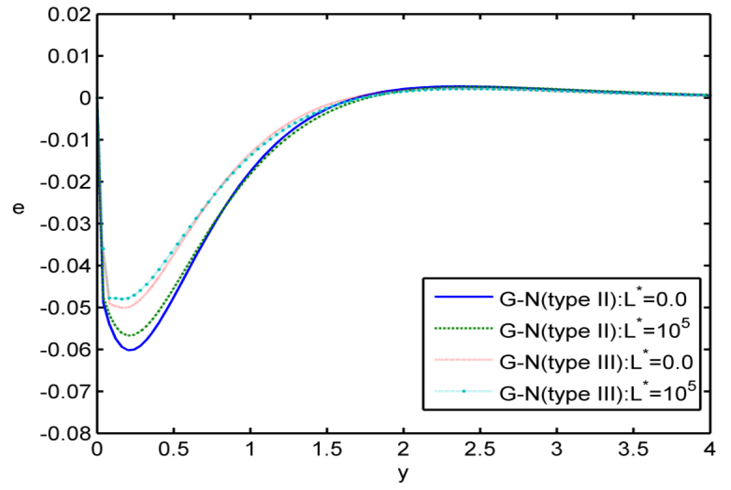
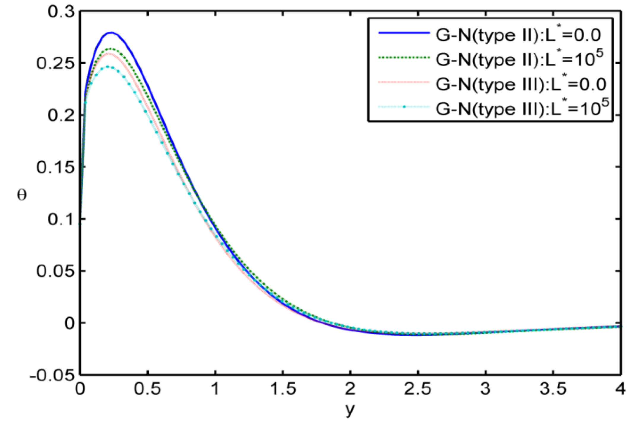
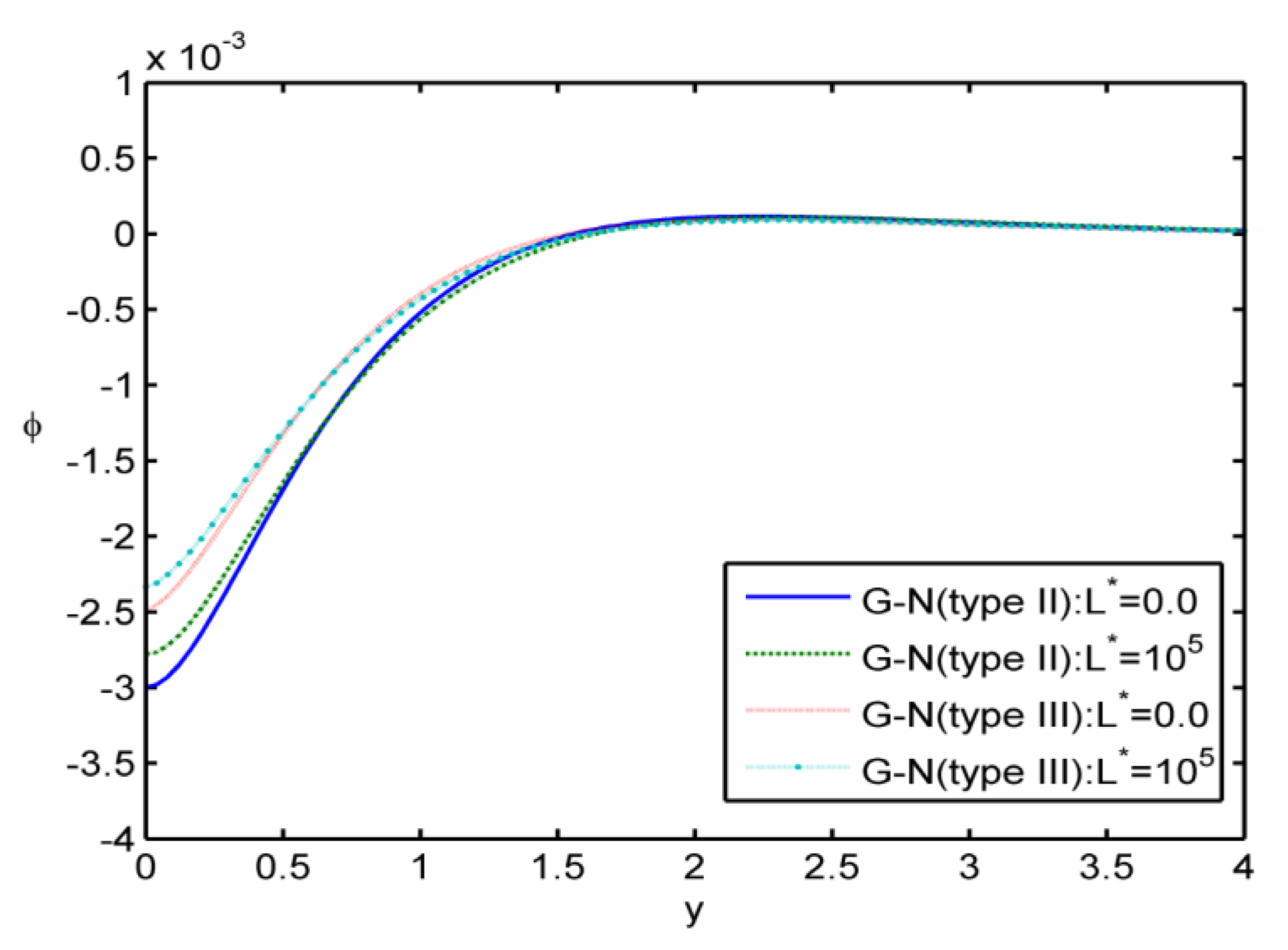
Case i: In the Figure 1, Figure 2, Figure 3 and Figure 4, we made the calculations for , at . The values of the deformation e, the values of the temperature the electromagnetic field , and the values of the voids function are graphically represented, for different values of y in some graphs of two-dimensional space. In these figures, we use the solid lines for the results in the case without initial stress for the (G-N) theory of type II. For the results in the case of the (G-N) theory of type II with initial stress, we have used the large dashes line. In the case without initial stress for the (G-N) theory of type III, we have used the small dashes. Finally, for the results in the case with initial stress for the (G-N) theory of type III, we have used the small dashes line with dot.
Figure 1 depicts the variation of the strain e versus y. The magnitude of the strain is found to be large for the G-N theory of type III. It can be seen that the initial stress shows an increasing effect on the magnitude of strain. In Figure 2, the parameter for the initial stress is decreasing as an effect. Additionally, when the initial stress parameter is increasing, the value of the temperature is decreasing. Figure 3 shows the variation of the induced magnetic field versus . The value of strain is found to be large for the theory of G-N of type III. It can be seen that the presence of the initial stress shows a decreasing effect on the magnitude of the induced magnetic field. Figure 4 expresses the distribution of the change in the volume fraction field versus . It was observed that the initial stress has a great effect on the distribution of .
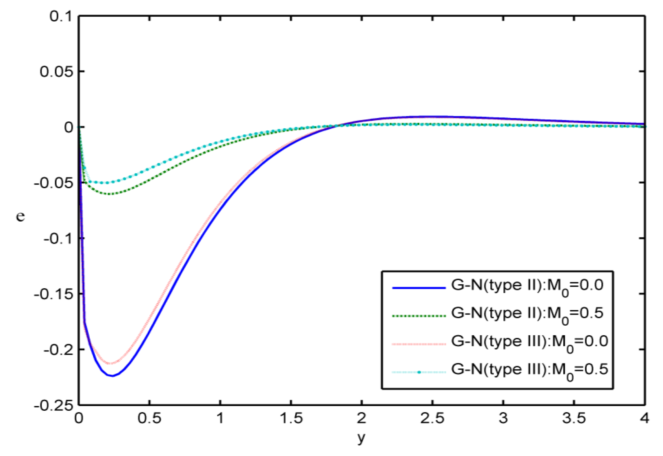
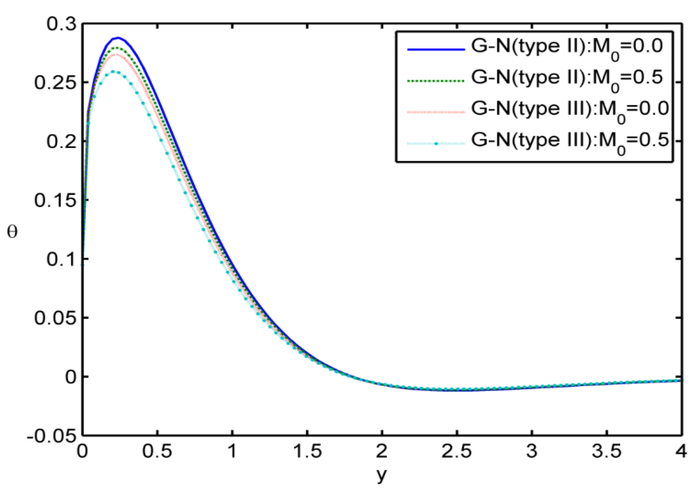
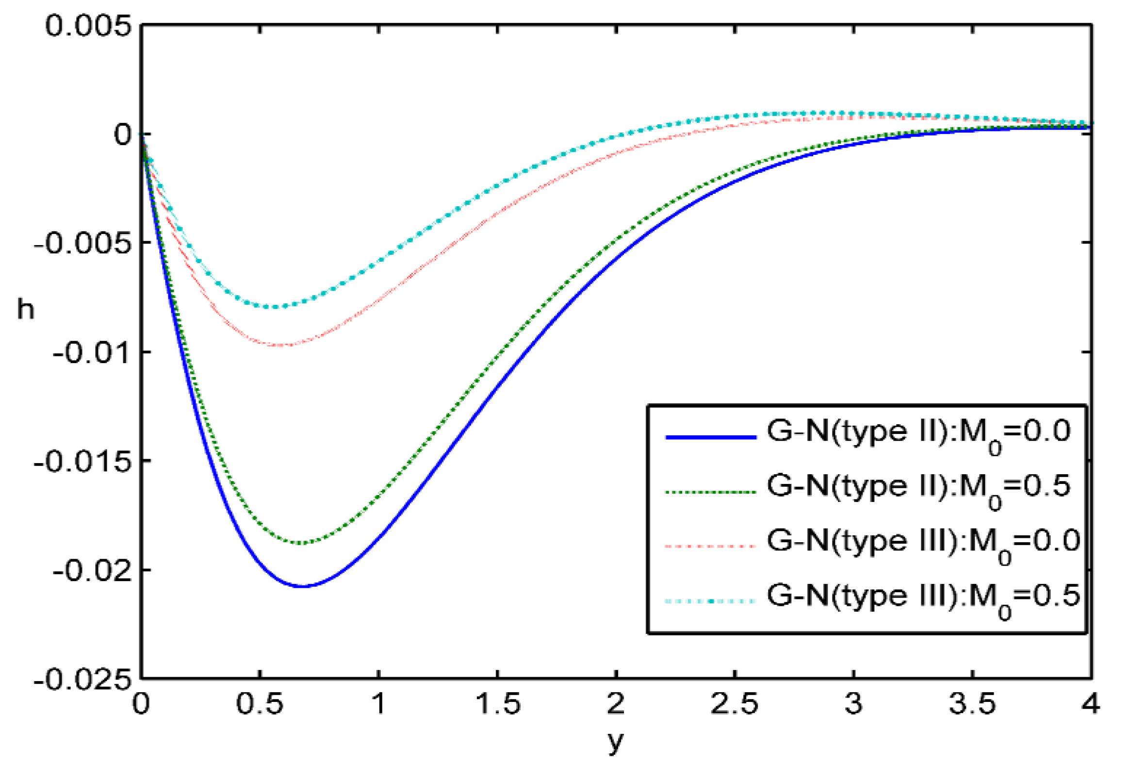
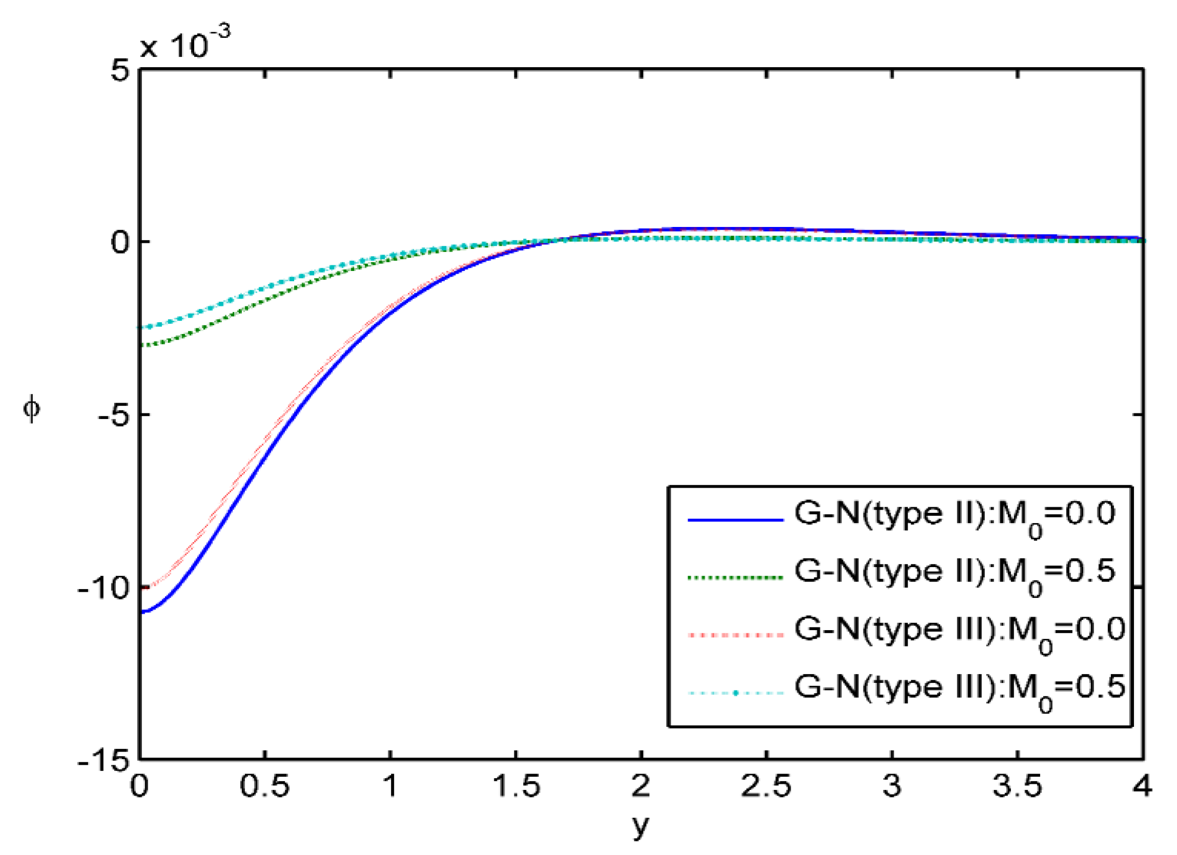
Case ii: In the Figure 5, Figure 6, Figure 7 and Figure 8, calculations were made for at , and . The strain e, the temperature , the electromagnetic field h and the voids function are graphically represented in some of the graphs for different values of y. Here, the solid lines is for results in the G-N theory of type II at , which gives the classical Fourier’s law of heat conduction, the large dashes line is for results in the type II G-N theory at , which gives the generalized Fourier’s law of heat conduction. We also use a small dashes line for the results for the type III G-N theory in the case , while the line with small dashes and the dot is for results for the type III G-N theory for . Figure 5 is for the effect of in the case that it exists and we can see that the value of the deformation e is increasing when increases with the corresponding difference. Figure 6 is for the value of the temperature , which is decreasing for the parameter , which is increasing. In Figure 7, the effect of parameter exists and the value of the induced magnetic field h increases when the parameter increases. In Figure 8, the value of the voids function is increasing for the case that the parameter is increasing.
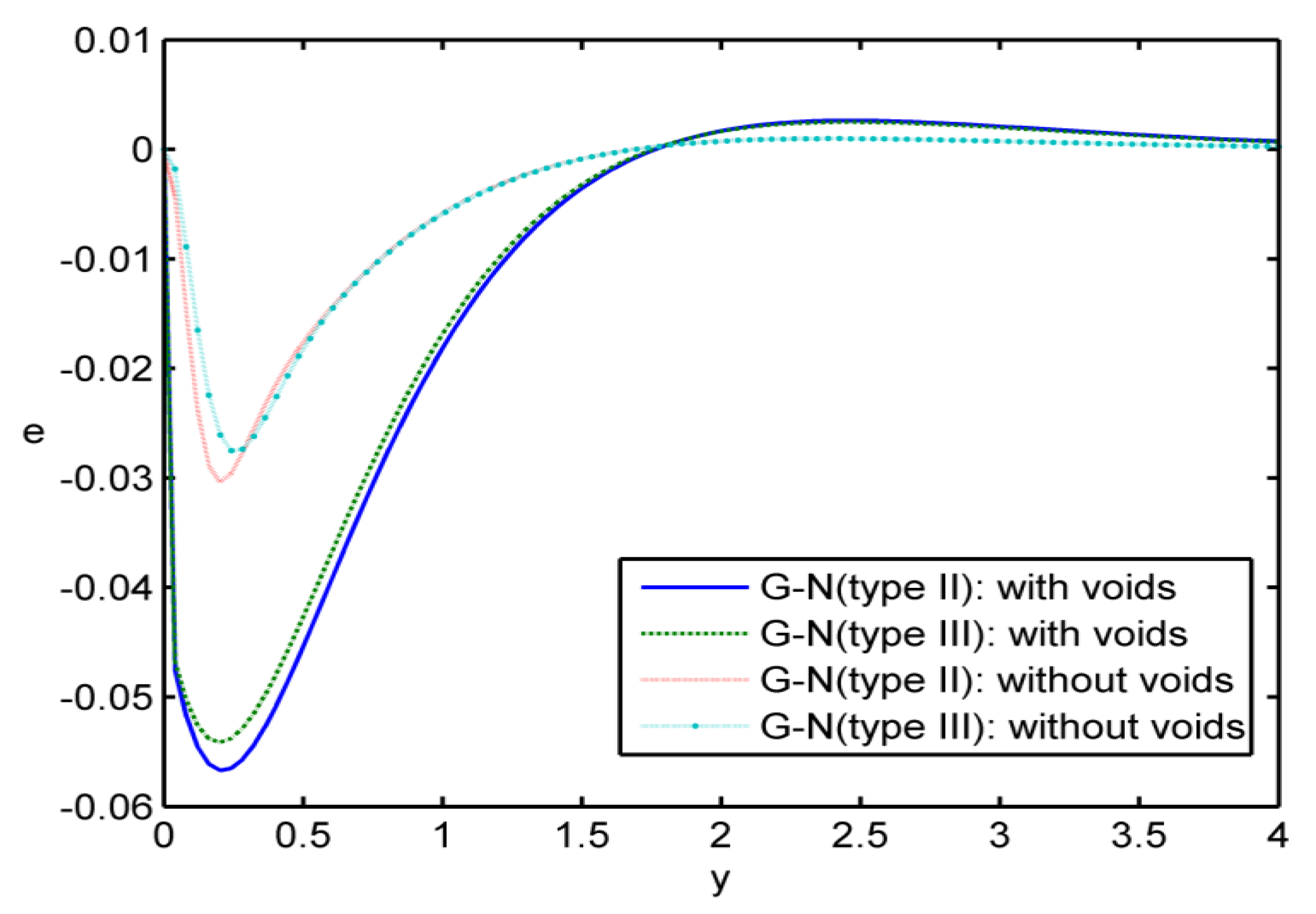
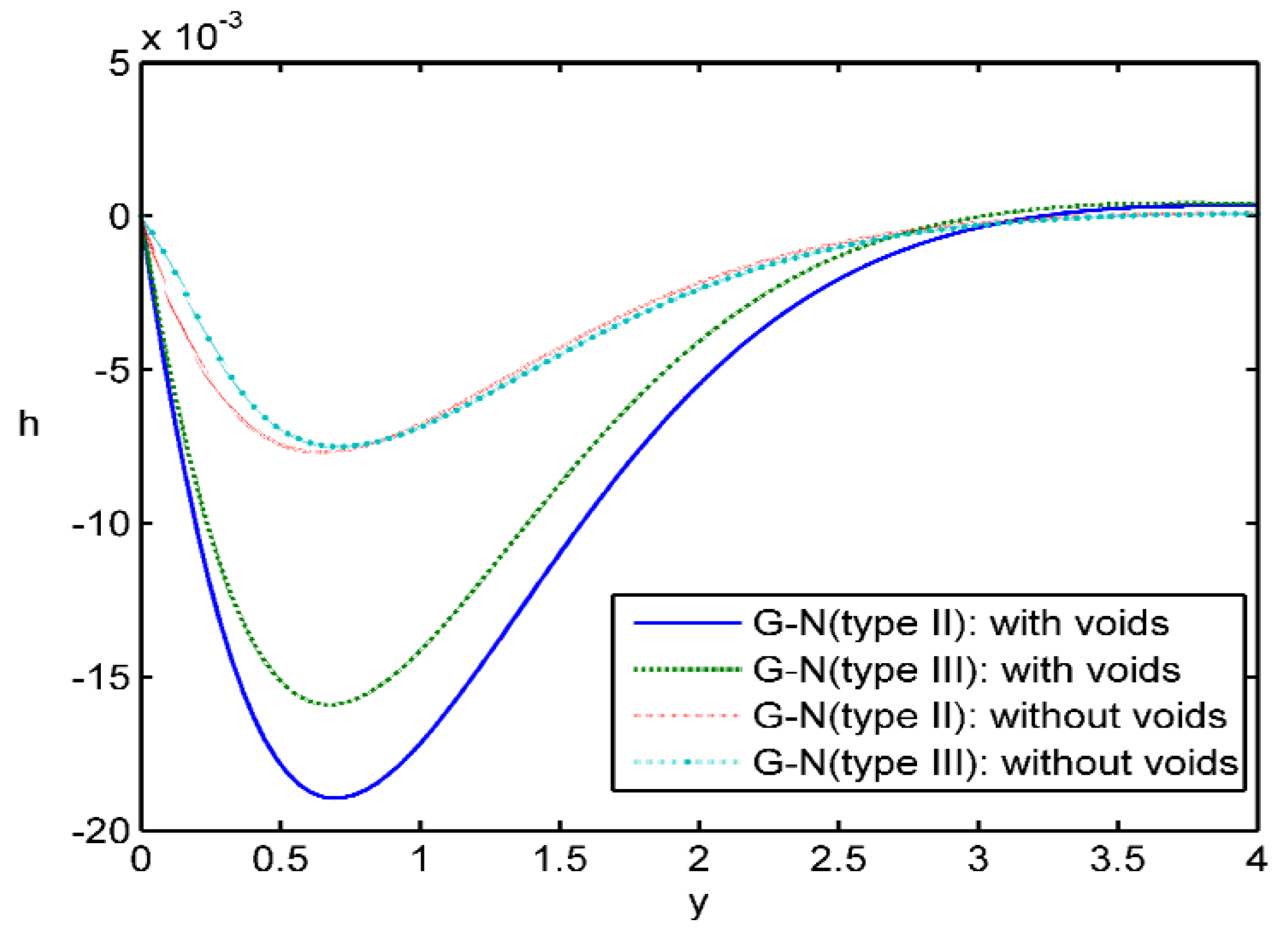
Case iii: Figure 9, Figure 10 and Figure 11 present the evolution of the physical sizes with regards to the distance in 2D during , , , and with and without void parameter, in the context of G-N theory of type II and type III G-N theories. In this case of comparison, the solid lines is for results of pore effect in the type II G-N theory, the small dashes line is also the voids effect, but in the case of the type III G-N theory. We use a large dashes line for results in the G-N theory of type II by neglecting the effect of pores, while the small dashes line with dot is used for results in the type III G-N theory, neglecting the effect of pores. In Figure 9, we find the repartition of the strain , and we have a comparison between the values of the strain in the case of the presence of the pores to those in the case of neglecting the voids, in the range ; while, the values are the same for two cases at . Figure 10 illustrates the repartition of the temperature and a comparison between the temperature in the case of presence of pores to those in the case of neglecting the voids, for y in the range 0 < y < 1.9. In the case y > 1.9, the values are the same for two cases. Figure 11 depicts the repartition of the magnetic field h, an the values of the magnetic field h in the case of the presence of pores are compared to those in the case of neglecting the voids, for y in the range ; in the case . The values are the same for the two cases.
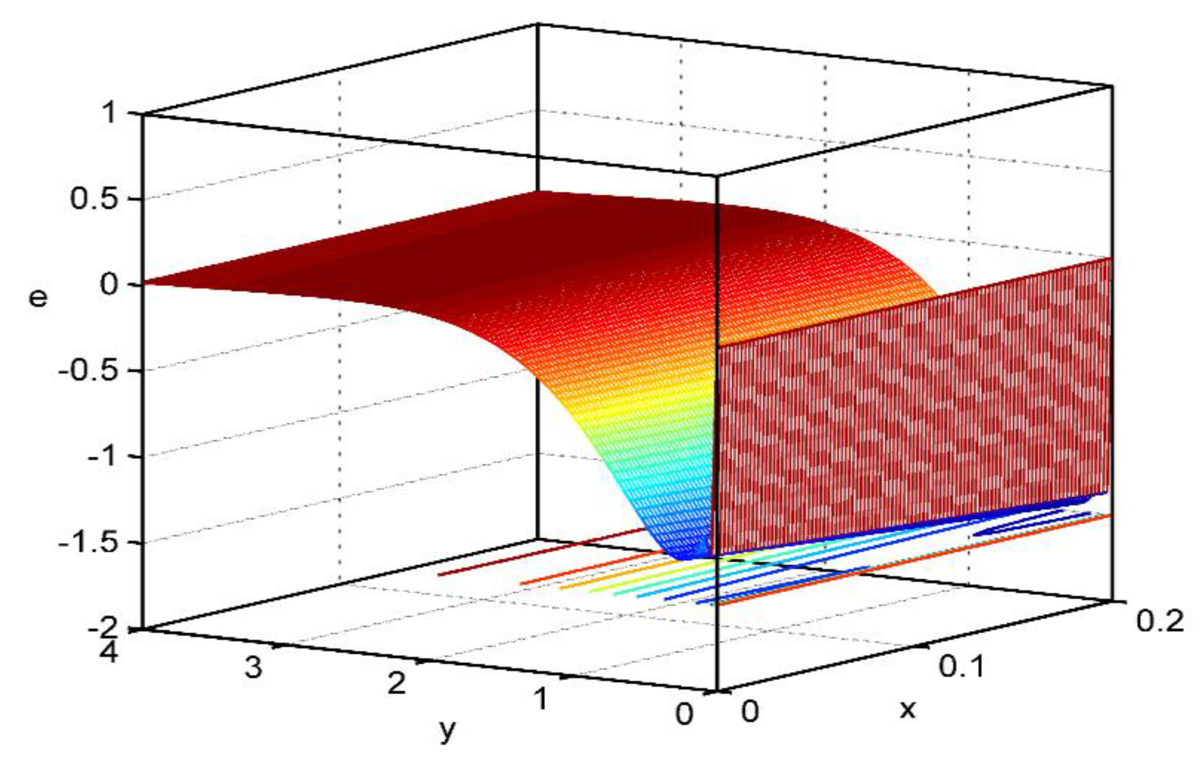
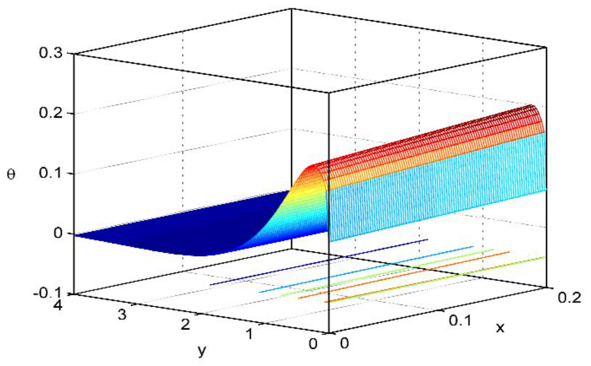
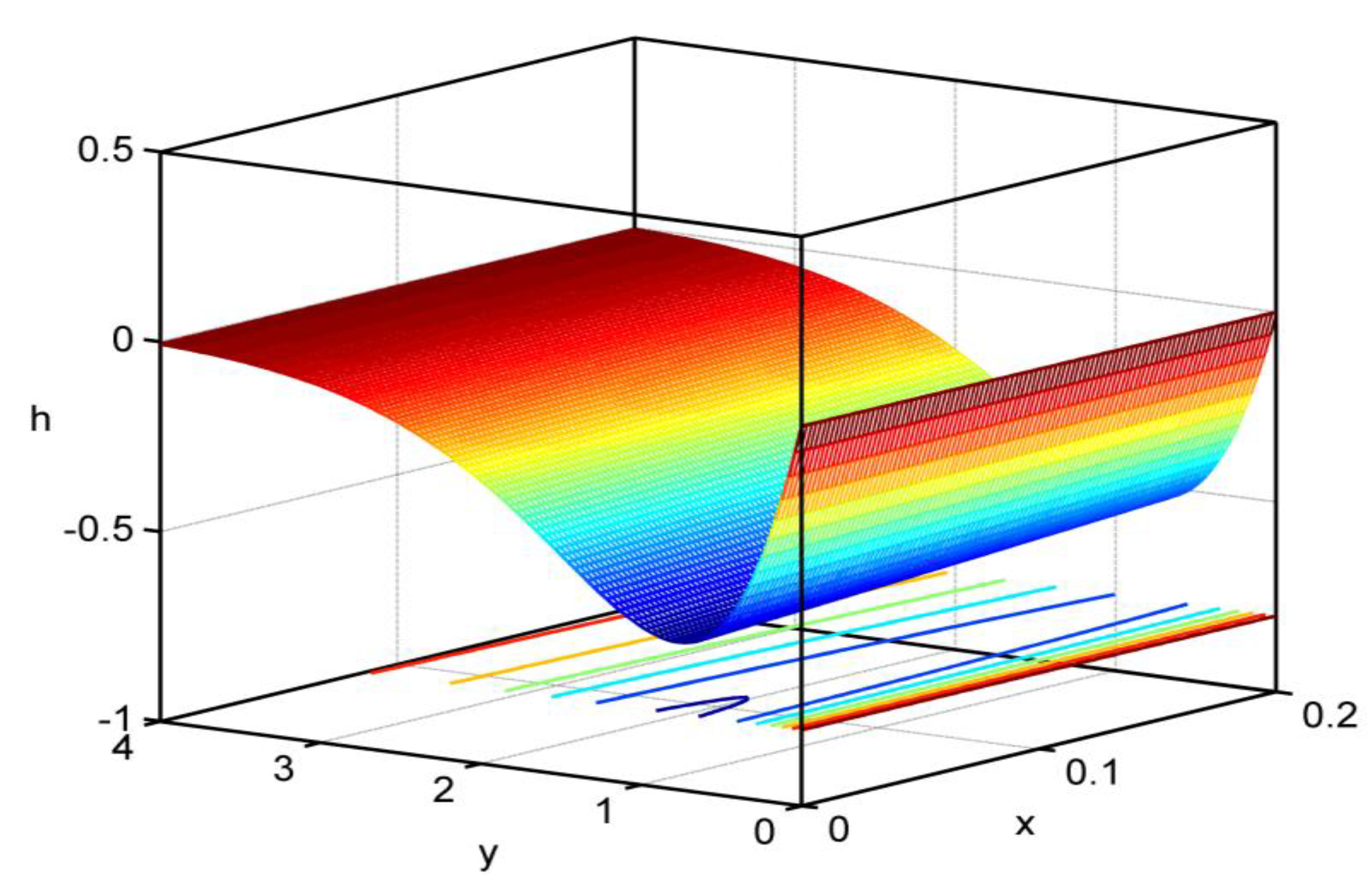
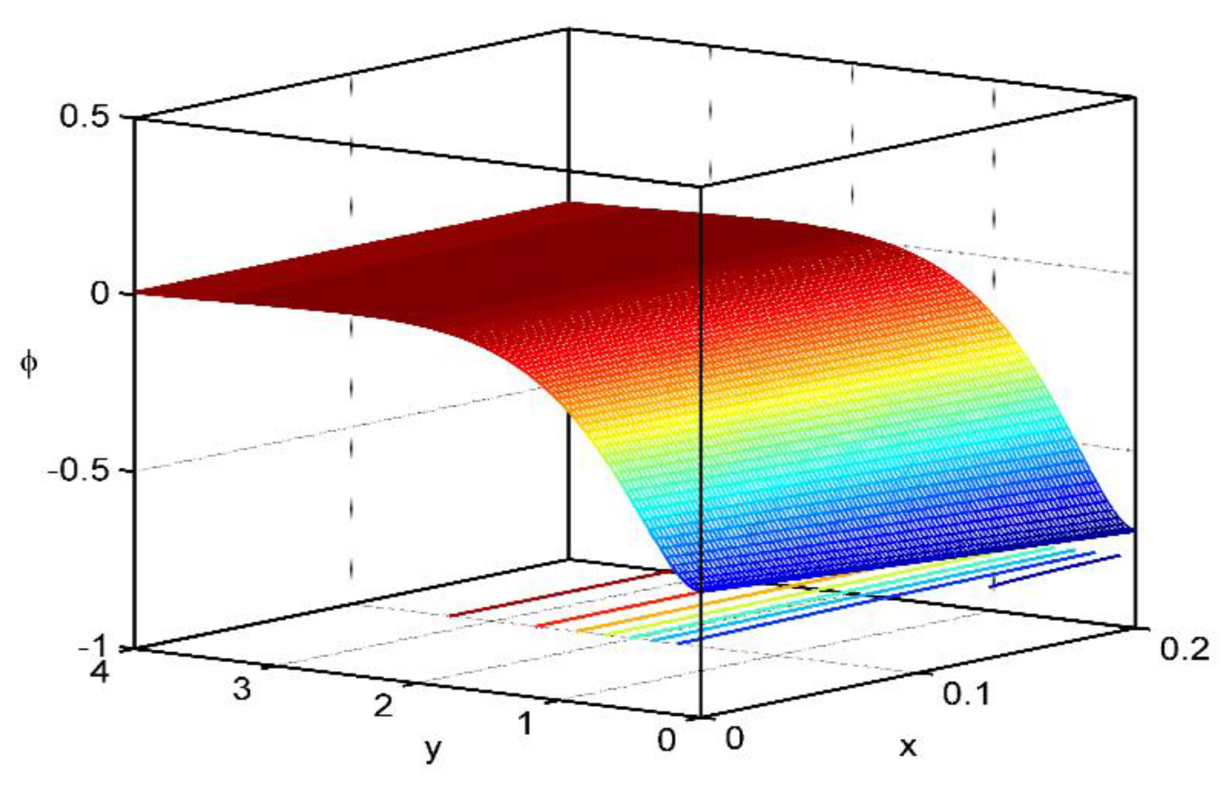
Figure 12, Figure 13, Figure 14 and Figure 15 are giving 3D surface curves for the physical quantities i.e., the strain e, the temperature , the magnetic field , and the voids fuction for the thermoelastic theory of electromagnetic bodies with pores, by taking into account the Thomson effect and the effect of the initial stress. The importance of these figures is that they give the dependence of the above physical sizes regarding the vertical component of distance.
6. Conclusions
The results concluded from the above analysis can be summarized, as follows:
- (1)
- We have derived the field equations of homogeneous, isotropic, electro-magneto-thermo- porous elastic half-plane with the Thomson effect and initial stress.
- (2)
- The analytical solutions that are based upon normal mode analysis for the thermoelastic problem in solids have been developed and utilized.
- (3)
- The presence of initial stress, void parameters, and Thomson effect play significant roles in all of the physical quantities.
- (4)
- The value of all physical quantities converges to zero with the increase in distance and all of the functions are continuous.
- (5)
- The deformation of a body depends on the nature of the applied forces and Thomson effect, as well as the type of boundary conditions.
Author Contributions
All three authors conceived the framework and structured the whole paper, checked the results of the paper and completed the revision of the article. The authors have equally contributed to the elaboration of this manuscript. All authors have read and approved the final manuscript.
Funding
This research received no external funding.
Acknowledgments
The authors would like to thank the anonymous referee for the comments that helped us improve this article.
Conflicts of Interest
The authors declare no conflict of interest.
References
- Green, A.E.; Naghdi, P.M. A re-examination of the basic postulates of thermo-mechanics. Proc. R. Soc. Lond. A 1991, 432, 171–194. [Google Scholar] [CrossRef]
- Green, A.E.; Naghdi, P.M. On undamped heat wave in elastic solids. J. Therm. Stresses 1992, 15, 253–264. [Google Scholar] [CrossRef]
- Green, A.E.; Naghdi, P.M. Thermoelasticity without energy dissipation. J. Elast. 1993, 31, 189–209. [Google Scholar] [CrossRef]
- Sharma, J.N.; Chouhan, R.N. On the problems of body forces and heat sources in thermoelasticity without energy dissipation, Indian. J. Pure Appl. Math. 1999, 30, 595–610. [Google Scholar]
- Liang, M.; Liu, Y.; Xiao, B.; Yang, S.; Wang, Z.; Han, H. An analytical model for the transverse permeability of gas diffusion layer with electrical double layer effects in proton exchange membrane fuel cells. Int. J. Hydrogen Energy 2018, 43, 17880–17888. [Google Scholar] [CrossRef]
- Xiao, B.; Zhang, X.; Wang, W.; Long, G.; Chen, H.; Kang, H.; Ren, W. Afractal model for water flow through unsaturated porous rocks. Fractals 2018, 26, 1840015. [Google Scholar] [CrossRef]
- Hassan, M.; Marin, M.; Alsharif, A.; Ellahi, R. Convective heat transfer flow of nanofluid in a porous medium over wavy surface. Phys. Lett. A Gen. At. Solid State Phys. 2018, 382, 2749–2753. [Google Scholar] [CrossRef]
- Long, G.; Liu, S.; Xu, G.; Won, S.W. A perforation-erosion model for hydraulic-fracturing applications. SPE Prod. Oper. 2018, 33, 770–783. [Google Scholar] [CrossRef]
- Xiao, B.; Chen, H.; Xiao, S.; Cai, J. Research on relative permeability of nanofibers with capillary pressure effect by means of fractal-monte Carlo technique. J. Nanosci. Nanotechnol. 2017, 17, 6811–6817. [Google Scholar] [CrossRef]
- Xiao, B.; Wang, W.; Fan, J.; Chen, H.; Hu, X.; Zhao, D.; Zhang, X.; Ren, W. Optimization of the fractal-like architecture of porous fibrous materials related to permeability, diffusivity and thermal conductivity. Fractals 2017, 25, 1750030. [Google Scholar] [CrossRef]
- Nunziato, J.W.; Cowin, S.C. A non-linear theory of elastic materials with voids. Arch. Rat. Mech. Anal. 1979, 72, 175–201. [Google Scholar] [CrossRef]
- Cowin, S.C.; Nunziato, J.W. Linear theory of elastic materials with voids. J. Elast. 1983, 13, 125–147. [Google Scholar] [CrossRef]
- Puri, P.; Cowin, S.C. Plane waves in linear elastic materials with voids. J. Elast. 1985, 15, 167–183. [Google Scholar] [CrossRef]
- Iesan, D. A theory of thermoelastic materials with voids. Acta Mech. 1986, 60, 67–89. [Google Scholar] [CrossRef]
- Cicco, S.D.; Diaco, M. A theory of thermoelastic material with voids without energy dissipation. J. Therm. Stress. 2002, 25, 493–503. [Google Scholar] [CrossRef]
- Othman, M.I.A.; Edeeb, E.R.M. The effect of rotation on thermoelastic medium with voids and temperature dependent under three theories. J. Eng. Mech. 2018, 144, 04018003. [Google Scholar] [CrossRef]
- Montanaro, A. On singular surfaces in isotropic linear thermoelasticity with initial stress. J. Acoust. Soc. Am. 1999, 106, 1586–1588. [Google Scholar] [CrossRef]
- Othman, M.I.A.; Abd-Elaziz, E.M. The effect of thermal loading due to laser pulse on generalized thermoelastic medium with voids in dual phase lag model. J. Therm. Stress. 2015, 38, 1068–1082. [Google Scholar] [CrossRef]
- Marin, M. Cesaro means in thermoelasticity of dipolar bodies. Acta Mechanica 1997, 122, 155–168. [Google Scholar] [CrossRef]
- Marin, M.; Oechsner, A. The effect of a dipolar structure on the Holder stability in Green-Naghdi thermoelasticity. Contin Mech Thermodyn 2017, 29, 1365–1374. [Google Scholar] [CrossRef]
- Nowinski, J. Theory of Thermoelasticity with Applications; Sijthoff and Noordhoff International Publishers: Alphen Aan Den Rijn, The Netherlands, 1978. [Google Scholar]
- Chadwick, P. Progress in Solid Mechanics; Hill, R., Sneddon, I.N., Eds.; North Holland Publishing Company: North Holland, Amsterdam, 1960. [Google Scholar]
- Hussain, F.; Ellahi, R.; Zeeshan, A. Mathematical models of electromagnetohydrodynamic multiphase flows synthesis with nanosized hafnium particles. Appl. Sci. 2018, 8, 275. [Google Scholar] [CrossRef]
- Bhatti, M.M.; Zeeshan, A.; Ellahi, R.; Ijaz, N. Heat and mass transfer of two-phase flow with Electric double layer effects induced due to peristaltic propulsion in the presence of transverse magnetic field. J. Mol. Liq. 2017, 230, 237–246. [Google Scholar] [CrossRef]
- Othman, M.I.A.; Abd-Elaziz, E.M. Plane waves in a magneto-thermoelastic solids with voids and microtemperatures due to hall current and rotation. Results Phys. 2017, 7, 4253–4263. [Google Scholar] [CrossRef]
- Marin, M.; Craciun, E.M.; Pop, N. Consideration on mixed initial-boundary value problems for micro-polarporous bodies. Dyn. Syst. Appl. 2016, 25, 175–196. [Google Scholar]
- Marin, M.; Craciun, E.M. Uniqueness results for a boundary value problem in dipolar thermoelasticity to model composite materials. Compos. Part B Eng. 2017, 126, 27–37. [Google Scholar] [CrossRef]
- Dhaliwal, R.S.; Singh, A. Dynamic Coupled Thermoelasticity; Hindustan Publ. Corp.: New Delhi, India, 1980. [Google Scholar]
Figure 1.
The strain distribution at and .

Figure 2.
The temperature distribution at and .

Figure 3.
The induced magnetic field distribution at , and .

Figure 4.
The change in the volume fraction field distribution at and .

Figure 5.
The strain distribution at and .

Figure 6.
The temperature distribution at and .

Figure 7.
The induced magnetic field distribution at and .

Figure 8.
The change in the volume fraction field distribution at and .

Figure 9.
The strain distribution at , and .

Figure 10.
The temperature distribution at , , and .

Figure 11.
The induced magnetic field distribution at , , and .

Figure 12.
Three-dimensional (3D) curve distribution of the strain versus the distances at: , , and .
Figure 12.
Three-dimensional (3D) curve distribution of the strain versus the distances at: , , and .

Figure 13.
3D Curve distribution of the temperature versus the distances, at: , and .

Figure 14.
3D Curve distribution of the induced magnetic field versus the distances, at: , and .

Figure 15.
3D Curve distribution of the change in the volume fraction field versus the distances, at: , and .
Figure 15.
3D Curve distribution of the change in the volume fraction field versus the distances, at: , and .

© 2019 by the authors. Licensee MDPI, Basel, Switzerland. This article is an open access article distributed under the terms and conditions of the Creative Commons Attribution (CC BY) license (http://creativecommons.org/licenses/by/4.0/).
Share and Cite
MDPI and ACS Style
Abd-Elaziz, E.M.; Marin, M.; Othman, M.I.A. On the Effect of Thomson and Initial Stress in a Thermo-Porous Elastic Solid under G-N Electromagnetic Theory. Symmetry 2019, 11, 413. https://0-doi-org.brum.beds.ac.uk/10.3390/sym11030413
AMA Style
Abd-Elaziz EM, Marin M, Othman MIA. On the Effect of Thomson and Initial Stress in a Thermo-Porous Elastic Solid under G-N Electromagnetic Theory. Symmetry. 2019; 11(3):413. https://0-doi-org.brum.beds.ac.uk/10.3390/sym11030413
Chicago/Turabian StyleAbd-Elaziz, Elsayed M., Marin Marin, and Mohamed I. A. Othman. 2019. "On the Effect of Thomson and Initial Stress in a Thermo-Porous Elastic Solid under G-N Electromagnetic Theory" Symmetry 11, no. 3: 413. https://0-doi-org.brum.beds.ac.uk/10.3390/sym11030413
Note that from the first issue of 2016, this journal uses article numbers instead of page numbers. See further details here.