An Overview of End-to-End Automatic Speech Recognition


1
Science and Technology on Parallel and Distributed Processing Laboratory, National University of Defense Technology, Changsha 410073, China
2
College of Computer, National University of Defense Technology, Changsha 410073, China
*
Authors to whom correspondence should be addressed.
Symmetry 2019, 11(8), 1018; https://0-doi-org.brum.beds.ac.uk/10.3390/sym11081018
Submission received: 30 June 2019
/
Revised: 21 July 2019
/
Accepted: 3 August 2019
/
Published: 7 August 2019
Abstract
:Automatic speech recognition, especially large vocabulary continuous speech recognition, is an important issue in the field of machine learning. For a long time, the hidden Markov model (HMM)-Gaussian mixed model (GMM) has been the mainstream speech recognition framework. But recently, HMM-deep neural network (DNN) model and the end-to-end model using deep learning has achieved performance beyond HMM-GMM. Both using deep learning techniques, these two models have comparable performances. However, the HMM-DNN model itself is limited by various unfavorable factors such as data forced segmentation alignment, independent hypothesis, and multi-module individual training inherited from HMM, while the end-to-end model has a simplified model, joint training, direct output, no need to force data alignment and other advantages. Therefore, the end-to-end model is an important research direction of speech recognition. In this paper we review the development of end-to-end model. This paper first introduces the basic ideas, advantages and disadvantages of HMM-based model and end-to-end models, and points out that end-to-end model is the development direction of speech recognition. Then the article focuses on the principles, progress and research hotspots of three different end-to-end models, which are connectionist temporal classification (CTC)-based, recurrent neural network (RNN)-transducer and attention-based, and makes theoretically and experimentally detailed comparisons. Their respective advantages and disadvantages and the possible future development of the end-to-end model are finally pointed out. Automatic speech recognition is a pattern recognition task in the field of computer science, which is a subject area of Symmetry.
Keywords:
automatic speech recognition; end-to-end; deep learning; neural network; CTC; RNN-transducer; attention; HMM1. Introduction
Popularity of smart devices has made people more and more feel the convenience of voice interaction. As a very natural human–machine interacting method, automatic speech recognition (ASR) has been an important issue in the machine learning field since the 1970s [1].
Automatic speech recognition’s task is to identify an acoustic input sequence of length T as a label sequence (generally are letters, words or Chinese characters) of length N. Here, is a D-dimensional speech input vector (such as the Mel Filter Bank) corresponding to the t-th speech frame, is labels’ vocabulary, is the label at position u in L. We use to represent the collection of all label sequences formed by labels in . The task of ASR is to find the most likely label sequence given X. Formally:
Therefore, the essential work of ASR is to establish a model that can accurately calculate the posterior distribution .
Automatic speech recognition is a pattern recognition task in the field of computer science, which is a subject area of symmetry.
In a large vocabulary continuous speech recognition task, the hidden Markov model (HMM)-based model has always been mainstream technology, and has been widely used. Even today, the best speech recognition performance still comes from HMM-based model (in combination with deep learning techniques). Most industrially deployed systems are based on HMM.
At the same time, deep learning techniques have also spurred the rise of an alternative, which is the end-to-end model. Compared with the HMM-based model, the end-to-end model uses a single model to directly map audio to characters or words. It replaces engineering process with learning process and needs no domain expertise, so end-to-end model is simpler for constructing and training. These advantages make the end-to-end model quickly become a hot research direction in large vocabulary continuous speech recognition (LVCSR).
In this paper we make a detailed review of end-to-end model. We make a brief comparison between HMM-based model and end-to-end model, introduce the development of end-to-end technology, thoroughly analyze different end-to-end technologies’ paradigms and compare their advantages and disadvantages. Finally, we give our conclusions and opinions of future works.
The following content of this paper is organized as follows: In Section 2, we briefly reviewed the history of automatic speech recognition, focus on introducing the basic ideas and characteristics of HMM-Gaussian mixed model (GMM), HMM-deep neural network (DNN), end-to-end models, and comparing their strengths and weaknesses; in Section 3, Section 4 and Section 5, we summarize and analyze the principles, progress and research focus of connectionist temporal classification (CTC)-based, recurrent neural network (RNN)-transducer and attention-based three different end-to-end models, respectively. Section 6 makes a theoretically and experimentally detailed comparison of these end-to-end models, and concludes their respective advantages and disadvantages. The possible future works of the end-to-end model are given in Section 7.
2. Background of Automatic Speech Recognition
2.1. History of ASR
Dreyfus Graf of France first started research related to speech recognition. He represented speech signal as the output of six band-pass filters and used its trace information displayed on screen to determine transcriptions [2].
In 1952, Bell Labs of the United States made the first truly complete speech recognizer [3], which could recognize 10 digits by matching filter bank output to hand-constructed template. Since then, the filter-based approach began to develop rapidly. In 1956, Olson and Belar developed a simple voice-activated typewriter [4]. At MIT Lincoln Labs built a speaker-independent 10-vowel recognizer [5].
Basically, speech recognition systems at this stage can only recognize speeches containing a single word or vowel.
In the 1960’s, several Japanese laboratories demonstrated their capability of building special purpose hardware to perform a speech recognition task [6]. Most notable were the vowel recognizer of Suzuki and Nakata at the Radio Research Lab in Tokyo [7], the phoneme recognizer of Sakai and Doshita at Kyoto University [8], and the digit recognizer of NEC Laboratories [9]. The work of Sakai and Doshita involved the first use of a speech segmenter for analysis and recognition of speech in different portions of the input utterance. In contrast, an isolated digit recognizer implicitly assumed that the unknown utterance contained a complete digit (and no other speech sounds or words) and thus did not need an explicit “segmenter”. Kyoto University’s work could be considered a precursor to a continuous speech recognition system [6].
Around 1970, Itakura, Saito, Atal, etc. first introduced linear prediction technology to speech study [10], and Vintsyuk et al. applied dynamic programming technology to speech recognition [11]. Atal and Itakura independently proposed the Linear Predictive Coding LPC) cepstrum distance [10,12]. These technologies’ introduction led to the rapid development of speech recognition for speaker-specific, isolated words and small vocabulary tasks.
With the satisfactory results of speech recognition for speaker-specific, isolated words and small vocabulary tasks, people began to extend speech recognition to LVCSR for non-specific-speaker speech. However, the changes in characteristics of non-specific-speaker voice, the context correlation within continuous speech, and the increase in vocabulary pose serious challenges to existing technologies [2].
For non-specific-speaker, large vocabulary continuous speech recognition tasks, HMM-based technology and deep learning technology are the key to its breakthrough.
In the mid-1980s, HMM technology based on statistics began to be widely studied and applied in speech recognition, and made substantial progress. Among them, the SPHINX system [13] developed by Kai-Fu Lee of Carnegie–Méron University, which uses HMM to model the speech state over time and uses GMM to model HMM states’ observation probability, made a breakthrough in LVCSR and is considered a milestone in the history of speech recognition. Until deep learning techniques were applied, HMM-GMM had been the dominant framework for speech recognition.
In the 1990s and early 2000s, the HMM-GMM framework was thoroughly and extensively researched. However, the recognition performance was also approaching its ceiling, especially when dealing with daily conversations such as telephone calls, conferences, etc., its performance is far from practical.
Recently, deep learning brings remarkable improvements in many researches such as community question answering [14] and visual tracking [15]. New development in speech recognition has also been promoted. In 2011, Yu Dong, Deng Li, etc. from Microsoft Research Institute proposed a hidden Markov model combined with context-based deep neural network which named context-dependent (CD)-DNN-HMM [16]. It achieved significant performance gains compared to traditional HMM-GMM system in LVCSR task. Since then, LVCSR technology using deep learning has begun to be widely studied.
2.2. Models for LVCSR
After years of development, LVCSR has made great progress. Many speech recognition systems are now deployed on mobile phones, televisions, and automobiles, playing a very important role in lives. Based on the differences in their basic ideas and key technologies, LVCSR can be divided into two categories: HMM-based model and the end-to-end model.
2.2.1. HMM-Based Model
For a long time, the HMM-based model has been the mainstream LVCSR model with the best recognition results. In general, the HMM-based model can be divided into three parts, each of which is independent of each other and plays a different role: acoustic, pronunciation and language model. The acoustic model is used to model the mapping between speech input and feature sequence (typically a phoneme or sub-phoneme sequence). The pronunciation model, which is typically constructed by professional human linguists, is to achieve a mapping between phonemes (or sub-phonemes) to graphemes. The language model maps the character sequence to fluent final transcription [17].
HMM mechanism may be used in all those three parts [18]. However, the HMM-based model generally emphasizes the use of HMM in acoustic model. In this HMM, sound is the observation, and feature is the hidden state. For an HMM that has a state set , HMM-based model uses Bayesian theory and introduces the HMM state sequence to decompose .
According to conditional independent hypothesis, we can approximate , therefore,
These three factors , , and in the Equation (3) correspond to acoustic model, pronunciation model, and language model, respectively.
- Acoustic model : It indicates the probability of observing X from hidden sequence S. According to the probability chain rule and the observation independence hypothesis in HMM (observations at any time depend only on the hidden state at that time), can be decomposed into the following form:In the acoustic model, is the observation probability, which is generally represented by GMM. The posterior probability distribution of hidden state can be calculated by DNN method. These two different calculations of result into two different models, namely HMM-GMM and HMM-DNN. For a long time, HMM-GMM model is a general structure for speech recognition. With the development of deep learning technology, DNN is introduced into speech recognition for acoustic modeling [19]. The role of DNN is to calculate the posterior probability of the HMM state, which may be transformed into likelihoods, replacing the conventional GMM observation probability [18]. Thus, HMM-GMM model is developed into HMM-DNN, which achieves better results than HMM-GMM and becomes state-of-the-art ASR model.
- Pronunciation model : this is also called the dictionary. Its role is to achieve the connection between acoustic sequence and language sequence. The dictionary includes various levels of mapping, such as pronunciation to phone, phone to trip-hone. The dictionary is not only used to achieve structural mapping, but also to map the probability calculation relationship.
- Language model : is trained by a large amount of corpus, using order Markov hypothesis to generate a m-gram language model.
In the HMM-based model, different modules use different technologies and play different roles. HMM is mainly used to do dynamic time warping at the frame level. GMM and DNN are used to calculate HMM hidden states’ emission probability [20]. The construction process and working mode of the HMM-based model determines if it faces the following difficulties in practical use:
- The training process is complex and difficult to be globally optimized. HMM-based model often uses different training methods and data sets to train different modules. Each module is independently optimized with their own optimization objective functions which are generally different from the true LVCSR performance evaluation criteria. So the optimality of each module does not necessarily mean the global optimality [21,22].
- Conditional independent assumptions. To simplify the model’s construction and training, the HMM-based model uses conditional independence assumptions within HMM and between different modules. This does not match the actual situation of LVCSR.
2.2.2. End-to-End Model
Due to the above-mentioned shortcomings of the HMM-based model, coupled with the promotion of deep learning technology, more and more works began to study end-to-end LVCSR. The end-to-end model is a system that directly maps input audio sequence to sequence of words or other graphemes. Its functional structure is shown in Figure 1.
Most end-to-end speech recognition models include the following parts: encoder, which maps speech input sequence to feature sequence; aligner, which realizes the alignment between feature sequence and language; decoder, which decodes the final identification result. Please note that this division does not always exist, because end-to-end itself is a complete structure, and it is usually very difficult to tell which part does which sub-task at the analogy of an engineered modular system.
Different from the HMM-based model that is composed of multiple modules, the end-to-end model replaces multiple modules with a deep network, realizing the direct mapping of acoustic signals into label sequences without carefully-designed intermediate states. Besides, there is no need to perform posterior processing on the output.
Compared to HMM-based model, the above differences give end-to-end LVCSR the following characteristics:
- Multiple modules are merged into one network for joint training. The benefit of merging multiple modules is that there is no need to design many modules to realize the mapping between various intermediate states [23]. Joint training enables the end-to-end model to use a function that is highly relevant to the final evaluation criteria as a global optimization goal, thereby seeking globally optimal results [22].
- It directly maps input acoustic signature sequence to the text result sequence, and does not require further processing to achieve the true transcription or to improve recognition performance [24], whereas in the HMM-based models, there is usually an internal representation for pronunciation of a character chain. Nevertheless, character level models are known with some traditional architectures, too.
These advantages of end-to-end LVCSR model make it able to greatly simplify the construction and training of speech recognition models.
To varying degrees, sequence-to-sequence tasks face data alignment problems, especially for speech recognition. Where a label in the label sequence should be aligned to the speech data is an unavoidable problem for both HMM-based and end-to-end model. The end-to-end model uses soft alignment. Each audio frame corresponds to all possible states with a certain probability distribution, which does not require a forced, explicit correspondence [22].
The end-to-end model can be divided into three different categories depending on their implementations of soft alignment:
- CTC-based: CTC first enumerates all possible hard alignments (represented by the concept path), then it achieves soft alignment by aggregating these hard alignments. CTC assumes that output labels are independent of each other when enumerating hard alignments.
- RNN-transducer: it also enumerates all possible hard alignments and then aggregates them for soft alignment. But unlike CTC, RNN-transducer does not make independent assumptions about labels when enumerating hard alignments, so it is different from CTC in terms of path definition and probability calculation.
- Attention-based: this method no longer enumerates all possible hard alignments, but uses Attention mechanism to directly calculate the soft alignment information between input data and output label.
3. CTC-Based End-to-End Model
Although currently the HMM-DNN hybrid model still has state-of-the-art results, the role played by DNN is limited. It is mostly used to model the posterior state probability of HMM’s hidden state, only representing local information. The time-domain feature is still modeled by HMM. When attempting to model time-domain features using RNN or CNN instead of HMM, it faces a data alignment problem: both RNN and CNN’s loss functions are defined at each point in the sequence, so in order to be able to perform training, it is necessary to know the alignment relation between RNN output sequence and target sequence [25].
CTC was proposed in [25]. Its emergence makes it possible to make fuller use of DNN in speech recognition and build end-to-end models, which is a breakthrough in the development of end-to-end method. Essentially, CTC is a loss function, but it solves hard alignment problem while calculating the loss. CTC mainly overcomes the following two difficulties for end-to-end LVCSR models:
- Data alignment problem. CTC no longer needs to segment and align training data. This solves the alignment problem so that DNN can be used to model time-domain features, which greatly enhances DNN’s role in LVCSR tasks.
- Directly output the target transcriptions. Traditional models often output phonemes or other small units, and further processing is required to obtain the final transcriptions. CTC eliminates the need for small units and direct output in final target form, greatly simplifying the construction and training of end-to-end model.
Solving these two problems, CTC can use a single network structure to map input sequence directly to label sequence, and implement end-to-end speech recognition.
3.1. Key Ideas of CTC
CTC process can be seen as including two sub-processes: path probability calculation and path aggregation. In these two sub-processes, the most important is the introduction of a new blank label (“-”, which means no output) and the intermediate concept path.
3.1.1. Path Probability Calculation
Given an input sequence of length T, the encoder encodes it into a feature sequence of length T, for any t, is a vector whose dimension is one more than the number of elements in the vocabulary , i.e., .
CTC acts on the feature sequence . Through softmax operation, CTC converts it into a probability distribution sequence , , where indicates the probability that the output at time step t is label i, indicates the probability of outputting the blank label at time step t.
Let , denote the collection of all sequences of length T that defined on the vocabulary . Combined with the definition of , we can conclude that for a given input sequence X, the conditional probability distribution of any sequence in the collection is calculated as Equation (6):
where represents the label at position t of sequence . The element in is called path and is represented by .
After the above calculation process, the input sequence is mapped to a path of the same length, and the conditional probability of can also be calculated according to Equation (6). In this mapping process, every input frame is mapped to a certain label . It can be thought as that the mapping from input sequence to path is actually a hard-aligning process.
From the calculation process of Equation (6), we can see that there is a very important assumption, which is the independence assumption: elements in the output sequence are independent of each other. Any time step which label is selected as the output does not affect the label distribution at other time steps. In contrast, in the encoding process, the value of is affected by the speech context information in both historical and future directions. That is to say, CTC uses conditional independence assumptions in language models, but not in acoustic models. Therefore, the encoder obtained by CTC training is essentially and totally an acoustic model, which does not have the ability to model language.
3.1.2. Path Aggregation
From the path probability calculation process, we can find that the output path’s length is equal to the input speech sequence’s, which is not in line with actual situation. Usually, the length of transcription is much shorter than that of corresponding speech sequence. Therefore, a many-to-one, long-to-short mapping is needed to aggregate multiple paths into a shorter label sequence.
Let denote the set of all label sequences defined on vocabulary whose length is less than or equal to T, and the path aggregation is defined as a map function . It maps paths in (i.e., path) to the real label sequence in . The path aggregation mainly consists of two operations:
- Merge the same contiguous labels. If consecutive identical labels appear in the path, merge them and keep only one of them. For example, for two different paths “c-aa-t-” and “c-a-tt-”, they are aggregated according to the above principles to give the same result: “c-a-t-”.
- Delete the blank label “-” in the path. Since label “-” indicates that there is no output, it should be deleted when the final label sequence is generated. The above sequence “c-a-t-”, after being aggregated according to the present principle, becomes final sequence “cat”.
In above aggregation process, “c-aa-t-” and “c-a-tt-” are two paths of length 7, and “cat” is a label sequence of length 3. Analysis shows that a label sequence may correspond to multiple paths. Assuming that “cat” is aggregated by paths of length 4, then “cat” contains seven different paths as shown by the Figure 2.
Lattice of these paths are shown in Figure 3. 1, 2, 3, and 4 in the figure represent time steps, and “-”, “c”, “a”, and “t” are corresponding output values. Along the arrows’ direction, each path starting at time step 1 and ending at time step 4 corresponds to a possible path of “cat”.
Besides to obtain the label sequence corresponding to these paths, the aggregation also aims to calculate the label sequence’s probability. We use to represent the set of all paths in corresponding to the label sequence L, then obviously, given the input sequence X, the probability of L can be calculated as given in Equation (7):
The calculation of has been given in the Equation (6).
Obviously, calculation of L’s probability is differentiable. Therefore, after obtaining the label’s probability, the gradient back propagation method can be used to train the model.
However, there is still a difficulty for the calculation of Equation (7). Although is easy to calculate, It is hard to determine which and how many paths from are included in . Therefore, this equation is not really used to calculate . Its truly operational calculation method is the forward-backward algorithm [25].
Although the mapping from input sequence to path is a hard alignment process, due to the existence of path aggregation, CTC does not insist that input and output must be explicitly aligned according to a certain path. In fact, the path is only an intermediate concept of probability calculation, and the segmentation alignment it represents does not really happen. Therefore, CTC actually uses a soft alignment method, which is essentially different from HMM-based model [22].
The emergence of CTC technology greatly simplifies the construction and training of LVCSR model. It no longer needs expertise to build various dictionaries; it eliminates the need of data alignment, allowing us to use any number of layers, any network structure to build an end-to-end model mapping audio directly to text [26].
3.2. CTC-Based Works
Since CTC’s calculation process is quite certain, Most of CTC-based ASR works mainly study how to effectively build the neural net acoustic model.
3.2.1. Model Structure
One of CTC’s great advantages is that it eliminates the necessity of data segmentation alignment, so that deep learning techniques such as CNN and RNN can play an increasingly important role. Network models with different structures and depths have been introduced into end-to-end ASR, and have achieved better and better results.
Ref. [26] proposed an end-to-end model trained by CTC for an LVCSR task. To the best of our knowledge, this is the first work in this area. It designed a three-layer network. The first layer is a 78-dimensional feed forward layer, the second layer is a 120-dimensional LSTM layer, and the third layer is a 27-dimensional LSTM layer. A CTC layer is used for training. The results of various structures showed that increasing network’s depth and hidden cell’s number could effectively improve the recognition effect. This conclusion was further confirmed by the experimental results in [27].
Based on the above conclusions, ef. [22] believed that the model of up to three LSTM layers was still too shallow, so it did not achieved remarkable results. This paper uses CTC technology to train a five-layer bidirectional LSTM model with 500 hidden units per direction in every layer. The recognition effect reached state-of-the-art level at the time. Encouraged by this work, many improvements to the five-layer network began to appear [19,28,29,30].
Since then, with the rapid development of deep learning technology, ASR model trained using CTC has also undergone great changes in structure and depth.
In terms of structure, ref. [31] introduced CNN and combined it with RNN for ASR. It designed the structure consists of four CNN layers, two dense layers, two RNN layer and a CTC layer. To solve the problem that almost all models use RNN which is difficult for training, ref. [21] designed a model that abandons RNN and only uses CNN and CTC. The model used a 10-layer CNN and a three-layer full connection, and performed convolution operations in both time and frequency dimensions. Results also showed that deeper models could lead to better recognition. But more importantly, they found that a CNN networks with sufficient layers could also model the time-domain characteristics.
In terms of network depth, ref. [32] made a bold attempt to train a network with nine layers (where seven layers are RNNs) using CTC. The model could even outperform a human in certain tasks. Ref. [33] used CTC to train a deep neural network model with seven layers of bidirectional LSTM with each direction having 1000 hidden units. It was trained on 125,000 h of voice data from YouTube, which had a transcription vocabulary of 100 K. Similarly, ref. [34] used CTC to train a neural network consisting of nine layers of bidirectional RNNs with hidden unit dimension of 1024, which achieved optimal results on their respective data sets.
However, the trend in network model’s structure and depth does not mean that deeper and more complex networks can achieve better results at any situation. Many newer jobs [35,36,37] chose to use shallower networks (five layers), which in large part were because that the dataset they use did not support training deeper networks. For example, ref. [35] used 2000-h datasets to train their five-layer model, while [33] used 125,000 data to train seven-layer networks. There is a huge gap between the two datasets.
3.2.2. Large-Scale Data Training
Lots of works show that complex, deep models require a lot of data to train, so as to speech recognition. Successful deep ASR models often benefit from a large-scale training data.
In order to effectively train a five-layer network model, the data set used by [19] has more than 7000 h of clean speech data, include their own 5000 h data and some other data sets (WSJ, Switchboard, Fisher). Coupled with the synthetic noise speech, there are totally more than 100,000 h of speech data used for training. With the help of large-scale datasets, they achieved the best results on their own constructed noisy datasets, outperforming several commercial companies such as Apple, Google, Bing, and wit.ai. In their further work, Ref. [32] used 11,940 h of English speech and 9400 h Chinese speech data to train the nine-layer network (seven layers are RNN) model, and finally achieved better level than human in regular Chinese recognition.
At Google’s works, Ref. [33] trained a seven-layer bi-directional LSTM using 125,000 h of voice data from YouTube, which has a transcription vocabulary of 100 K. Their other work [38] used 125,000 h of google voice-search traffic data for experiments, too.
A large amount of training data helps to improve model’s performance, but in order to use so many data, training method needs to be improved accordingly.
In order to speed up the training procedure on large-scale data, ref. [19] made special designs from two aspects: data parallelism and model parallelism. In terms of data parallelism, the model used intra-graphics processing unit (GPU) parallelism, with each GPU processing multiple samples simultaneously. Data parallelism was also performed between GPUs, where multiple GPUs independently process one minibatch and finally integrate their gradients together. In addition, training data were sorted by length so that audios of the same length are in the same minibatch, reducing the average processing steps of RNN. In terms of model parallelism, the model was divided into two parts according to the time series and run separately. For bi-directional RNN, the two parts exchanged their roles and respective calculation results at the intermediate time points, thus improving RNN’s calculation speed.
Based on [19,32] designed following efficient methods for large-scale data training at a more fundamental level: (1) it created its own all-reduce open message passing interface (OpenMPI) code to sum gradients from different GPUs on different nodes; (2) it designed an efficient CTC calculation method to run on GPU; (3) it designed and used a new memory allocation method. Finally, the model achieved 4–21 times acceleration.
3.2.3. Language Model
Equation (6) indicates that CTC considers each label in the output sequence to be independent of each other. This independent assumption makes CTC not capable of modeling languages. Therefore, many CTC-based works use a variety of methods to add a language model to CTC. Their results show that language model is very helpful for improving the performance of CTC-based end-to-end ASR.
Ref. [22] showed that on the WSJ dataset, RNN+CTC model alone had 30.1% word error rate (WER). If a word dictionary was introduced, the WER was 24%. If a tri-gram language model (LM) was introduced, the WER fell to 8.7%. Ref. [28] also showed that a language model was essential to achieve good performance at the word level.
Inspired by these works, ref. [27,29,39,40] and other works also integrated language model with CTC. Results showed that the language model can greatly improve recognition accuracy. Not only that, but the language model is also effective even for models with complex structure and large training data such as DeepSpeech [19] and Deepspeech2 [32]. In contrast, there are less works that do not use language model [21,34], which are less accurate than works with language model.
There are two main ways to use the language model: second-pass and first-pass. Second-pass is also known as re-ranking or the re-score method. In this method, the model first uses a beam-search algorithm to obtain a certain number of candidate results based on the probability distribution calculated by CTC. These results are then re-scored by the language model, and both of the two scores are used to determine the optimal recognition result [22]. The first-pass method adds the language model score at every extending step in beam-search, and only needs to run the scoring process once to get the final result. Since language model is integrated into the beam-search process, the first-pass method generally has better results and has been more widely used.
However, introducing language model also has its shortcomings. On the one hand, introduction of language model makes the CTC-based works deviate from the end-to-end principle, and the characteristics of joint training using an individual model are destroyed. The language model only works in the prediction phase and does not help the training process. On the other hand, the language model is very large. For example, the seven-gram language model used in [29] is 21 GB, which has a great impact on model’s deployment and delay.
4. RNN-Transducer End-to-End Model
There are two main deficiencies in CTC, which limits its effectiveness:
- CTC cannot model interdependencies within the output sequence because it assumes that output elements are independent of each other. Therefore, CTC cannot learn the language model. The speech recognition network trained by CTC should be treated as only an acoustic model.
- CTC can only map input sequences to output sequences that are shorter than it. For scenarios where output sequence is longer, CTC is powerless. This can be easily analyzed from CTC’s calculation process.
For speech recognition, it is clear that the first point has a greater impact. RNN-transducer was proposed in the paper [41]. It designs a new mechanism to solve above-mentioned shortcomings of CTC. Theoretically, it can map an input to any finite, discrete output sequence. Interdependencies between input and output and within output elements are also jointly modeled.
4.1. Key Ideas of RNN-Transducer
The RNN-transducer, which is a model structure, has many similarities with CTC which is a loss function: their goals are to solve the forced segmentation alignment problem in speech recognition; they both introduce a “blank” label; they both calculate the probability of all possible paths and aggregate them to get the label sequence. However, their path generation processes and the path probability calculation methods are completely different. This gives rise to the advantages of RNN-transducer over CTC.
RNN-transducer model consists of three subnetworks: Transcription network (), Prediction network () and joint network (). Its structure is shown in Figure 4. These three networks have their own functions:
- Transcription network (): this is the encoder, which plays the role of an acoustic model. Regardless of sub sampling technique, for an acoustic input sequence of length T, map it to a feature sequence . Correspondingly, for input value at any time t, Transcription network is used as an acoustic model with an output value , which is a dimensional vector.
- Prediction network (): It’s part of the Decoder that plays the role of language model. As an RNN network, it models the interdependencies within output label sequence (while transcription network models the dependencies within acoustic input). maintains a hidden state and an output value for any label location . Their loop calculation process isLater in the analysis of joint networks we will point out that the calculation of depends on . So the above loop process actually means using the output sequence in the first positions to determine the choice of . For simplicity, we can express this relationship as . is also a dimension vector.
- Joint network (): it does the alignment job between input and output sequence. For any , , the joint network uses the transcription network’s output and the prediction network’s output to calculate the label distribution at output location u:As we can see, is a function of and . Since comes from , comes from the sequence , so the joint network’s role is: for a given historical output sequence and input at time t, it calculates the label distribution at the output location u, which provides probability distribution information for decoding process.
Based on , RNN-transducer designs its own path generation process and path aggregation method, and gives the corresponding forward-backward algorithm to calculate the probability of a given label sequence [41]. Since there exists a path aggregation process, RNN-Transducer is also a soft-aligned process that does not require forced, explicit split alignment of data.
The decoding process of RNN-transducer is roughly as follows: each time an input is read, the model will keep outputting labels until an empty label “-” is encountered. If an empty label is encountered, RNN-transducer reads in the next input and repeats the output process until all input sequences have been read. Since an input may produce an output subsequence more than one label, RNN-transducer can handle situations where the output’s length is greater than the input’s.
From RNN-transducer’s design ideas, we can easily draw the following conclusions:
- Since one input data can generate a label sequence of arbitrary length, theoretically, the RNN-transducer can map input sequence to an output sequence of arbitrary length, whether it is longer or shorter than the input.
- Since the prediction network is an RNN structure, each state update is based on previous state and output labels. Therefore, the RNN-transducer can model the interdependence within output sequence, that is, it can learn the language model knowledge.
- Since Joint Network uses both language model and acoustic model output to calculate probability distribution, RNN-Transducer models the interdependence between input sequence and output sequence, achieving joint training of language model and the acoustic model.
This work was tested at TIMIT (Texas Instruments, Inc. (TI) and the Massachusetts Institute of Technology(MIT)) corpus of read speech [42] and achieved a 23.2% PER (Phoneme Error Rate), which was the best in existing RNN model at that time, catching up with the best results.
4.2. RNN-Transducer Works
To further enhance RNN-transducer’s performance, ref. [43] improved the work from [41]. It changed the Joint network from original simple addition to a full layer connection. it also increased network depth and pre-trained the transcription network and the prediction network respectively. In the end, it got 17.7% PER (Phoneme Error Rate)at TIMIT dataset, which was the best result at the moment. A number of experimental comparisons showed that it was more difficult to train RNN-Transducer from scratch. Pre-training of RNN-transducer’s various parts could effectively improve the model’s effect.
Ref. [17] explored and improved the RNN-transducer in more ways. On the one hand, it used more layers to construct a model with a transcription network of 12 LSTM layers and a prediction network of two LSTM layers. On the other hand, it used hierarchical pre-training with CTC to output phonemes, fonts, and words on the fifth, 10th, and 12th layers of transcription network, respectively. At the same time, it no longer used word as its output unit, but usde word piece (which is the result of word segmentation or combination, may be a part of a word, or a combination of multiple words). In the end, it achieved 8.5% WER on Google Voice Search.
Although the RNN-Transducer has its advantages over CTC, in order to obtain this advantage, it also leads to other shortcomings. One obvious problem is that it allows many unreasonable paths to appear. Since the RNN-transducer is very flexible, allowing one input to produce multiple outputs, it is conceivable that such an extreme case may exist: the first audio frame produces all the output sequences, while all the other audio frames produce empty labels. This is obviously very unreasonable, but it is a situation that RNN-transducer will definitely include. There are lots of paths like this. To solve this problem, a recurrent neural aligner was proposed in [44,45]. This is an improvement to the RNN-transducer that restricts only one output per input. But even so, there are still unreasonable paths.
Analysis and related works on the RNN-transducer show that although the RNN-transducer has some improvements compared to CTC, it has the following shortcomings:
- Experiments show that the RNN-transducer is not easy to train. Therefore, it is necessary for each part to be pre-trained, which is very important for improving performance.
- Thd RNN-transducer’s calculation process includes many obviously unreasonable paths. Even if there are some improving works, it is still unavoidable. In fact, all speech recognitions that first enumerate all possible paths and then aggregate them face this problem, including CTC.
5. Attention-Based End-to-End Model
In 2014, ref. [46] published a work on machine translation. Their purpose was to solve the problem that the encoder-decoder model for machine translation was required to encode input texts into a fixed-length vector, resulting in limited encoding capability. In this work, the model’s encoder encoded input text into a sequence of vectors (rather than a single vector), and the decoder used an attention method at each output step to assign different weights to each vector in this sequence. The next-step output was determined by historical output sequence and a weighted summation of the encoding result sequence. This method solves the problem of having to encode all the text information into a fixed length vector, so that even a long sentence can have a good encoding effect. This work has greatly promoted speech recognition because it fits well with speech recognition tasks in the following ways:
- Speech recognition is also a sequence-to-sequence process that recognizes the output sequence from the input sequence. So it is essentially the same as translation task.
- The encoder–decoder method using an attention mechanism does not require pre-segment alignment of data. With attention, it can implicitly learn the soft alignment between input and output sequences, which solves a big problem for speech recognition.
- Encoding result is no longer limited to a single fixed-length vector, the model can still have a good effect on long input sequence, so it is also possible for such model to handle speech input of various lengths.
Based on the above reasons, end-to-end speech recognition model using attention mechanism has received more and more interests and development.
Attention-based end-to-end model can also be divided into three parts: encoder, aligner, and decoder. In particular, its aligner part uses attention mechanism. structure of attention-based model is shown in Figure 5. Different works will make different improvements to each part.
5.1. Works on the Encoder
The encoder plays the role of acoustic model, which is same as in CTC-based, RNN-Transducer and even HMM-DNN hybrid models. So it faces the same problems as they do, and their solutions are also the same. However, when the encoder is combined with attention, some new problems arise.
5.1.1. Delay and Information Redundancy
A serious problem caused by the combination of the encoder and attention is latency. Since attention is applied to the entire encoding result sequence, it needs to wait until the encoding process has been totally finished before it can start running (while CTC and RNN-transducer do not need to wait), so the time spent in the encoding process will increase the model’s delay. In addition, an encoder that does not shrink the sequence’s length will have a encoding result sequence that is much longer than the target label sequence (for input speech sequence is much longer than transcription). This leads to two problems: on the one hand, a longer encoding result sequence means more attention calculation, thereby increasing the delay; on the other hand, since speech is much larger than transcription, the sequence generated by encoding process without sub sampling will introduce a lot of redundant information to the attention mechanism. Being a work about translation task itself, ref. [46] does not take into account the sequence length problem which occurs in speech recognition task. In fact, early works [47,48] that use attention for speech recognition did not notice this issue either.
The first work to notice this problem and take action is [49]. It was based on their previous work [48]. The encoder part used pooling between multiple RNN layers to speed up the model by pooling in time dimension, which can reduce the input sequence’s length. The encoder’s time step between upper and lower layers was decremented by the proportion of , and the decrement could be realized by either an adjacent summation or a simple sub sampling. The model’s encoder used a four-layer bidirectional gated recurrent unit (GRU) [50], the last two layers read an output from previous layer every other time step, reducing the input to of its original length. This method is called pooling or sub sampling.
For the same purpose of reducing encoding result sequence’s length, the listen, attend and spell (LAS) [51] in 2016 adopted another operation. Its encoder part is called Listener and consists of 4 bidirectional LSTM layers. In order to reduce RNN’s loop steps, each layer used the concatenation of state of two consecutive time steps from previous layer as its input. This 4-layer RNN is called a pyramid structure and can reduce RNN loop steps to . Since then, most works used sub sampling or pyramid structure in their encoders. Some of them reduced the length to [52,53,54,55,56], some reduced to [57].
In addition, there is a technique that directly sub samples the input speech sequence before encoding it (directly operate on the input frame) [58,59,60]. Through these different sub sampling methods, the length of encoder’s result sequence is shortened, and the retained information is also filtered, which alleviates the model delay problem and the information redundancy problem in Attention.
5.1.2. Network Structure
Similar to the development trend in CTC-based and RNN-transducer models, in order to improve encoding ability, the encoder in attention-based models is also becoming more and more complicated. The most obvious point is reflected in its depth. The early encoder was basically within three layers [48,52,53,61], and gradually developed to four layers [49,51,54,57], five layers [59,62], six layers [55,60]. As the network structure becomes more complex and network’s depth becomes deeper, model’s effect is continuously improving. Based on [49], ref. [56] built a 15-layer encoder network using Network in Network, Batch normalization, residual network, convolutional LSTM, and ultimately achieved WER (Word Error Rate)of 10.53% on the WSJ (Wall Street Journal)dataset without using a dictionary or language model.
5.2. Works on Attention
Functionally, the attention mechanism can be divided into three types: content-based, location-based, and hybrid. The calculation process of their attention weights at the output position u is shown in Equation (12). They use different information in attention process and have different characteristics.
- Context-based: it uses only the input feature sequence F and the previous hidden state to calculate the weight at each position. Ref. [46] used this method. Its problem is that it does not use position information. For a feature’s different appearances in the feature sequence, context-based attention will give them same weights, which is called similarity speech fragment problem.
- Location-based: the previous weight is utilized as location information at each step to calculate current weight . But since it does not use the input feature sequence F, it is not sufficient for input features.
- Hybrid: as the name implies, it takes into account the input feature sequence F, the previous weight , and the previous hidden state , which enables it to combine advantages of context-based and location-based attention.
Based on the attention mechanisms of these different structures and functions, there are many works to solve different problems in speech recognition.
5.2.1. Continuity Problem
In translation tasks, It is a normal phenomenon two adjacent words in the result sequence may correspond to locations far away in the original sequence, and two words that are far apart in the resulting sequence may correspond to adjacent parts of the original sequence. But this phenomenon does not occur in speech recognition. The sound production process naturally determines that the two adjacent words in the transcription must correspond to adjacent parts in the audio. This is the continuity of speech recognition. To address continuity issues location-based or hybrid attention mechanisms need to be designed.
Based on [46,47] made some improvements to the attention mechanism to solve continuity problem. The improved attention process is:
Here and are two functions that need to be learned in training process. It can be seen that, the Equations (13) and (14) respectively use , f and in their calculating, so this is a hybrid attention. Compared to context-based, the Equation (14) introduces , which is used to penalize the attention weights according to the relative offset between the current and previous position, thereby solving the continuity problem.
5.2.2. Monotonic Problem
Another problem associated with continuity is the monotonic problem: sound is unidirectional in time dimension. Once we determine that an audio piece corresponds to a specific output label, then it is impossible for this piece to correspond to another label. That is: if a piece of audio has already been matched to a certain label through attention, when we identify subsequent labels, this audio piece should be excluded and not be considered.
In particular, one output label may appear many times in different locations in the transcription. They should be matched to different parts of the speech. However, during the calculation process they are likely to attend on the same speech part. This problem can also be solved by introducing location information in attention mechanism.
The solution proposed by [47] is to introduce some new loss terms into the training objectives:
Here, is the cumulative probability distribution function of the output label at position u up to time step t. represents the weight of feature at time step j for generating position u’s label. Obviously, the earlier the attention weight is, the more times it is calculated in . Therefore, the Equation (17) can make attention weight of position u more distributed to late time than that of position , thus having time monotonicity.
5.2.3. Inaccurate Extraction of Key Information
In 2014, ref. [46] found that the attention-based model can only be used to recognize audio data that has similar length with training data. Once the audio is significantly longer than the data used for training, performance would drop dramatically. Their follow-up work [48] once again validated this experimental phenomenon. Ref. [48] believed that reasons for this problem lied in the following aspects: first, the attention mechanism did not use location information; second, the attention mechanism could not attend on the real key features.
According to Equations (19)–(21), we can infer that , obviously this is a hybrid attention mechanism. But unlike general hybrid attention, it used convolution (∗ operation in the Equation (19)) to process location information.
For the second problem, ref. [48] believed that it was the following characteristics of softmax operation which was used to calculate the weight that caused the attention to fail to effectively focus on the really useful feature sequence:
- In the weights calculated by softmax, every item is greater than zero, which means that every feature of the feature sequence will be retained in the context information obtained by attention. This introduces unnecessary noise characteristics and retains some information that should not be retained in .
- Softmax itself concentrates the probability on the largest item, causing attention to focus mostly on one feature, while other features that have positive effects and should be retained are not fully preserved.
In addition, since the attention weights needs to be calculated for each feature in the feature sequence at each output step, the amount of calculation is large. In order to solve these problems, it proposed three sharpen techniques:
- It introduced a scale value greater than unity in softmax operation, which can enlarge greater weight and shrink smaller one. This method can attenuate the problem of noise characteristics, but makes the probability distribution more concentrated to the feature items with higher probability.
- After having calculated the weight of softmax, it only retains the largest k values and then normalizes them again. This method increases the amount of attention calculation.
- Window method. A calculation window and a window sliding strategy are set in advance, and attention’s weights are calculated by softmax only for data in the window.
It used the third method, only used in inference phase, not in training phase. The work finally achieved 17.6% WER at TIMIT. For sentences that are manually stitched and expanded to 10 times in length, The WER was still as low as 20%.
On this basis, these authors have made persistent efforts, and [49] has made further improvements to [48]: window technology was used not only in the inference phase but also in the training phase. Moreover, the window technology is different from that in [48]. In [48], the choice of new window depends on the previous moment’s window quality, so at the beginning the model is difficult to train, and easy to fall into local optimum. The adjustment strategy of [49] weakens this dependency. Its window initialization is performed according to the statistics of blank voice length and speaking speed in training data, which improves the performance.
5.2.4. Delay
There are two sources for the delay. On the one hand, the encoder’s result sequence is too long, which causes the attention and decoder to take a lot of time and computation. This problem has been alleviated by sub-sampling in the encoder. The other source is that the attention acts on the whole encoding result sequence, so it must wait until all the encoding result sequence are generated before it can start to work. In order to solve this problem, researchers also carried out a lot of exploration.
With the goal of reducing latency, ref. [52] attempted to build an online ASR system. On the one hand, it used a uni-directional RNN to build the encoder. On the other hand, the model used window mechanism proposed in [49] in attention. The advantage of using window mechanism is that attention no longer needs to wait until the end of entire encoding process, as long as it receives enough information that fulfill a window, it can start working. In this way, the attention’s delay can be controlled within a window.
Specifically, when the model performs attention at position u, it first calculates a window as follows.
In the attention process the model only considers appearing in the window (Reflected in the following equation is that the value of j is limited to )).
Also using window technology, ref. [61] believed that window size in existing window scheme was fixed, which was not consistent with actual situation. So it designed a window technology using Gaussian prediction method. Window’s size and slide step’s length are calculated based on the system state at corresponding time, rather than being set in advance. This kind of scheme can even adapt to the speed change to a certain extent.
Its Gaussian prediction window attention is roughly as follows:
Here, and are the Gaussian distribution mean and variance, respectively, which represent the position and size of the window at position u. It seems that the calculation of occurs on the entire encoding result sequence, but all outside the window are 0, so it actually only happens for , which greatly reduces the delay and implements a dynamic window.
5.3. Works on Decoder
The decoder is usually an RNN network that receives context information computed by attention and then decodes it to get the final transcription. Structurally, the decoder has two working modes in the existing work. One is to use previous hidden state to perform attention on encoding result sequence F, get the context information firstly, and then calculate the decoder’s current hidden state according to [47,58,61]. The other is to calculate the decoder’s current hidden state firstly, and then perform the attention on encoding result sequence to calculate the context information . The latter method has been used more widely. [48,49,51,52,53,56,59].
A lot of work has tried to improve attention-based ASR performance from the perspective of decoder.
Ref. [58] found that, in general, the decoder had only a one-layer network, and was not specifically designed for language features. So they designed the following decoder:
Compared to the traditional decoder structure, this work added the network layer shown by the Equation (36). This layer only acts on the historical output sequence, so it implicitly acts as a language model, which also allows the Decoder to have a longer memory.
Ref. [55] designed a multi-head-decoder technology for decoding. In the multi-header, different attention mechanisms are used on the encoding result sequence for context extraction and decoding. Results of these multiple attention decoding processes are aggregated to obtain the final decoding output.
The continuity, monotonicity, etc. of the attention mechanism naturally do not exist in CTC because CTC itself requires continuity and monotonicity of soft alignment between input and output. Ref. [54] attempted to combine CTC and attention in the training and inferring process to solve these problems for attention. It combined CTC and attention by sharing the encoder between them and extending the training loss function to , which taking into account the loss of CTC and attention. For decoding, the probability of CTC and attention were also jointly considered.
As a simulation of how humans perceive the world, the attention mechanism has been deeply studied in ASR. New problems are constantly emerging and solutions are constantly being proposed. However, lots of experimental works show that the attention-based model can achieve better results in ASR than CTC-based and RNN-transducer model.
6. Comparison and Conclusions
6.1. Model Characteristics Comparison
Table 1 compares these three end-to-end models in several aspects.
- Delay: the forward-backward algorithm used by CTC can adjust the probability of decoding results immediately after receiving a encoding result without waiting for other information, so CTC-based model has the shortest delay. RNN-Transducer model is similar to CTC in that it also adjusts the probability of decoding results immediately after each acquisition of an encoding result. However, since it uses not only the encoding result but also the previous decoding output in the forward-backward calculation at each step, its delay is higher compared to CTC. But, they all support streaming speech recognition, where recognition results are generated the same time speech signals are produced. Attention-based model has the longest delay because it needs to wait until all the encoding results are generated before soft alignment and decoding can start. So streaming speech recognition is not supported unless some corresponding compromise is made.
- Computational complexity: In the process of calculating the probability of L of length N based on X of length T, CTC technology needs to do a softmax on each input time step with a complexity of . RNN-transducer technology requires a softamx operation on each input/output pair with a complexity of . The primitive attention, like RNN-transducer, also requires a softamx operation on each input/output pair with complexity. However, as more and more attention mechanism uses window mechanisms, attention-based model only needs to perform softmax operation on the input segments in the window when outputting each label, and its complexity is reduced to , .
- Language modeling capabilities: CTC assumes that output labels are independent of each other, so it has no ability to model language. RNN-transducer enables models with language model ability through the joint network, while attention-based models achieves this through decoder network.
- Training difficulty: CTC is essentially a loss function, and there is no weight to train in itself. Its role is to train an acoustic model. Therefore, the CTC-based network model can quickly achieve optimal results. Attention mechanism and the joint network in RNN-transducer model introduce weights and functions that require training, and because of the joint training of language model and acoustic model, they are much more difficult to train than CTC-based models. In addition, RNN-transducer’s joint network will generate a lot of unreasonable data alignment between input and output. So it is more difficult to train than attention-based models. Generally, it needs to pre-train the prediction network and transcription network to have better performance.
- Recognition accuracy: due to the modeling of linguistic knowledge, recognition accuracies of RNN-Transducer and attention-based model are much higher than that of CTC-based model. In most cases, the accuracy of attention-based model is higher than RNN-transducer.
6.2. Model Recognition Performance Comparison
In order to analyze the advantages and disadvantages of various ASR methods, [38] designed experiments to carefully compare CTC-based, RNN-transducer, and attention models.
In these experiments, the input acoustic signal is represented with 80-dimensional log-mel features, computed with a 25 ms window, and a 10 ms frame-shift. Following previous work [30], three consecutive frames are stacked and only every third stacked frame are presented as input to the encoder. The same acoustic frontend is used for all experiments.
All models use characters as the output unit. The vocabulary includes 26 English lowercase letters, 10 Arabic numerals, a label representing ‘space’, and punctuation symbols (e.g., the apostrophe symbol (’), hyphen (-), etc.).
For end-to-end models, the encoders use five bi-directional long short time memory (BLSTM) [63] layers with 350 dimensions per direction. The decoders use a beam search decoding method with a width of 15. No additional language models or pronunciation dictionaries are used in decoding or re-scoring.
A CTC model is trained to predict characters as output targets. When trained to convergence, the weights from this encoder are used to initialize the encoders in all other sequence-to-sequence models, since this was found to significantly speed up convergence.
RNN-transducer’s Prediction network consists of a single 700-dimensional GRU, and its Joint network consists of a single 700-dimensional forward network with a tanh activation function. Attention’s Decoder also uses a 700-dimensional GRU, but both 1 layer and two-layer models are tested in these experiments.
Baseline used for comparison is the state-of-the-art context-dependent phoneme CTC model (CD-phoneme model). Its acoustic model consists of five layers of 700-dimensional bidirectional or unidirectional LSTM, predicting 8192 CD-phoneme Distribution. The baselines are first trained to optimize the CTC-criterion, followed by discriminative sequence training to optimize the state-level minimum Bayes risk (sMBR) criterion [64]. These models are decoded using a pruned, first-pass, five-gram language model which is subsequently rescored with a large five-gram language model. These systems use a vocabulary which consists of millions of words, as well as a separate expert-curated pronunciation model.
The various sequence-to-sequence modeling approaches are evaluated on an LVCSR task. In order to effectively train deep networks, it use a set of about 15 M hand-transcribed anonymized utterances extracted from Google voice-search traffic, which corresponds to about 12,500 h of training data. In order to improve system robustness to noise and reverberation, multi-condition training (MTR) data are generated: training utterances are artificially distorted using a room simulator, by adding in noise samples extracted from YouTube videos and environ mental recordings of daily events; the overall signal to noise (SNR) is between 0 dB and 30 dB, with an average of 12 dB.
The data used for test consists of three categories, which consist of hand-transcribed anonymized utterances extracted from Google traffic: a set of about 13,000 utterances (covering about 124,000 words) from the domain of open-ended dictation (denoted by dict); a set of about 12,900 utterances (covering about 63,000 words) from the domain of voice-search queries (denoted by vs); and a set of about 12,600 utterances (covering about 75,000 words) corresponding to instances of times, dates, etc., where the expected transcript corresponds to the written domain (denoted by numeric) (e.g., the spoken domain utterance “twelve fifty one pm” must be recognized as “12:51 p.m.”). Noisy versions of the dictation and voice-search sets are created by artificially adding noise drawn from the same distribution as in training (denoted, noisy-dict, and noisy-vs, respectively).
Table 2 gives the performance (WER) of different models on different test datasets.
Comparing the performance of different end-to-end models, we can get the following conclusions:
- Without external language model, CTC-based model has the worst effect, and the gap between it and other models is very large. This is consistent with our analysis and expectation of CTC: it makes a conditional independent assumption of the output and cannot learn language model knowledge itself.
- Compared with CTC, RNN-transducer has been greatly improved on all test sets because compared to CTC, it uses Prediction network to learn language knowledge.
- Attention-based model is the best of all end-to-end, and the two-layer decoder is better than the one-layer Decoder. This shows that decoder’s depth also has an impact on the results.
Although the end-to-end model has beat HMM-GMM model, lots of works show that its performance is still worse than HMM-DNN model [20,27,29,39,48,52,58], and some works achieve comparable performance with HMM-DNN model [45,47,54]. While only few works can outperform HMM-DNN model [23] (DeepSpeech [19] also outperforms HMM-DNN, however, it is trained on a large amount of data while HMM-DNN is not, which is unfair for comparison).
So, it is obvious that the end-to-end model has not surpassed the HMM-DNN model which also uses deep learning techniques. A very important reason is their different abilities to learn language knowledge. Although RNN-transducer and attention-based model have the ability to learn language models, the language knowledge they learn is only within the scope of training data set’s transcriptions. But HMM-DNN model is different. It uses specially constructed dictionaries and large language models trained on a large amount of extra natural language corpus. Its linguistic knowledge can have a very wide coverage.
As a conclusion, after years of development, the HMM-GMM model has reached its bottleneck, and there is little room for its further performance improvement. The introduction of deep learning technology has promoted the rise and development of HMM-DNN models and end-to-end models, which have achieved performance beyond HMM-GMM. Both using deep learning techniques, current performance of the end-to-end model is still worse than that of the HMM-DNN model, at best just comparable. However, the HMM-DNN model itself is limited by various unfavorable factors such as independent hypothesis and multi-module individual training inherited from HMM, while the end-to-end model has advantages such as simplified model, joint training, direct output, No need for forced data alignment. Therefore, the end-to-end model is the current focus of LVCSR and an important research direction in the future.
7. Future Works
The end-to-end model has surpassed the HMM-GMM model, but its performance is still worse than or only comparable to the HMM-DNN model, which also uses deep learning techniques. In order to truly take advantage of the end-to-end model, the end-to-end model needs to at least be improved in the following aspects:
- Model delay. CTC-based and RNN-transducer models are monotonic and support streaming decoding, so they are suitable for online scenarios with low latency. However, their recognition performance is limited. Attention-based models can effectively improve the recognition performance, but it is not monotonous and has long delay. Although there are methods such as “window” to reduce the delay of attention, they may reduce the recognition performance to a certain extent [65]. Therefore, reducing latency while ensuring performance is an important research issue for the end-to-end model.
- Language knowledge learning. HMM-based model uses additional language models to provide a wealth of language knowledge, while all the language knowledge of the end-to-end model comes only from training data’s transcriptions, whose coverage is very limited. This leads to great difficulties in dealing with scenes with large linguistic diversity. Therefore, the end-to-end model needs to improve its learning of language knowledge while maintaining the end-to-end structure.
Author Contributions
Conceptualization, D.W., X.W. and S.L.; funding acquisition, X.W. and S.L.; investigation, D.W.; methodology, D.W.; project administration, X.W.; supervision, X.W. and S.L.; writing—original draft, D.W.; writing—review and editing, X.W. and S.L.
Funding
This research was funded by the Fund of Science and Technology on Parallel and Distributed Processing Laboratory (grant number 6142110180405).
Conflicts of Interest
The authors declare no conflict of interest.
Abbreviations
The following abbreviations are used in this manuscript:
| LPC | Linear predictive coding |
| TIMIT | Texas Instruments, Inc. and the Massachusetts Institute of Technology |
| PER | Phoneme error rate |
| WSJ | Wall street journal |
| HMM | Hidden Markov model |
| GMM | Gaussian mixed model |
| DNN | Deep neural network |
| CTC | Connectionist temporal classification |
| RNN | Recurrent neural network |
| ASR | Automatic speech recognition |
| LVCSR | Large vocabulary continuous speech recognition |
| CD | Context-dependent |
| CNN | Convolutional neural network |
| LSTM | Long short time memory |
| GPU | Graphics processing unit |
| OpenMPI | Open message passing interface |
| LM | Language model |
| WER | Word error rate |
| LAS | Listen, attend and spell |
| CDF | Cumulative distribution function |
| BLSTM | Bi-directional long short time memory |
| GRU | Gated recurrent unit |
References
- Bengio, Y. Markovian models for sequential data. Neural Comput. Surv. 1999, 2, 129–162. [Google Scholar]
- Chengyou, W.; Diannong, L.; Tiesheng, K.; Huihuang, C.; Chaojing, T. Automatic Speech Recognition Technology Review. Acoust. Electr. Eng. 1996, 49, 15–21. [Google Scholar]
- Davis, K.; Biddulph, R.; Balashek, S. Automatic recognition of spoken digits. J. Acoust. Soc. Am. 1952, 24, 637–642. [Google Scholar] [CrossRef]
- Olson, H.F.; Belar, H. Phonetic typewriter. J. Acoust. Soc. Am. 1956, 28, 1072–1081. [Google Scholar] [CrossRef]
- Forgie, J.W.; Forgie, C.D. Results obtained from a vowel recognition computer program. J. Acoust. Soc. Am. 1959, 31, 1480–1489. [Google Scholar] [CrossRef]
- Juang, B.H.; Rabiner, L.R. Automatic speech recognition–a brief history of the technology development. Georgia Inst. Technol. 2005, 1, 67. [Google Scholar]
- Suzuki, J.; Nakata, K. Recognition of Japanese vowels—Preliminary to the recognition of speech. J. Radio Res. Lab. 1961, 37, 193–212. [Google Scholar]
- Sakai, T.; Doshita, S. Phonetic Typewriter. J. Acoust. Soc. Am. 1961, 33, 1664. [Google Scholar] [CrossRef]
- Nagata, K.; Kato, Y.; Chiba, S. Spoken digit recognizer for Japanese language. Audio Engineering Society Convention 16. Audio Engineering Society. 1964. Available online: http://www.aes.org/e-lib/browse.cfm?elib=603 (accessed on 4 August 2018).
- Itakura, F. A statistical method for estimation of speech spectral density and formant frequencies. Electr. Commun. Jpn. A 1970, 53, 36–43. [Google Scholar]
- Vintsyuk, T.K. Speech discrimination by dynamic programming. Cybern. Syst. Anal. 1968, 4, 52–57. [Google Scholar] [CrossRef]
- Atal, B.S.; Hanauer, S.L. Speech analysis and synthesis by linear prediction of the speech wave. J. Acoust. Soc. Am. 1971, 50, 637–655. [Google Scholar] [CrossRef] [PubMed]
- Lee, K.F. On large-vocabulary speaker-independent continuous speech recognition. Speech Commun. 1988, 7, 375–379. [Google Scholar] [CrossRef]
- Tu, H.; Wen, J.; Sun, A.; Wang, X. Joint Implicit and Explicit Neural Networks for Question Recommendation in CQA Services. IEEE Access 2018, 6, 73081–73092. [Google Scholar] [CrossRef]
- Chen, Z.Y.; Luo, L.; Huang, D.F.; Wen, M.; Zhang, C.Y. Exploiting a depth context model in visual tracking with correlation filter. Front. Inf. Technol. Electr. Eng. 2017, 18, 667–679. [Google Scholar] [CrossRef]
- Dahl, G.E.; Yu, D.; Deng, L.; Acero, A. Context-dependent pre-trained deep neural networks for large-vocabulary speech recognition. IEEE Trans. Audio Speech Lang. Process. 2011, 20, 30–42. [Google Scholar] [CrossRef]
- Rao, K.; Sak, H.; Prabhavalkar, R. Exploring architectures, data and units for streaming end-to-end speech recognition with RNN-transducer. In Proceedings of the 2017 IEEE Automatic Speech Recognition and Understanding Workshop (ASRU), Okinawa, Japan, 16–20 December 2017; pp. 193–199. [Google Scholar] [CrossRef]
- Lu, L.; Zhang, X.; Cho, K.; Renals, S. A study of the recurrent neural network encoder-decoder for large vocabulary speech recognition. In Proceedings of the Sixteenth Annual Conference of the International Speech Communication Association, Dresden, Germany, 6–10 September 2015; pp. 3249–3253. [Google Scholar]
- Hannun, A.; Case, C.; Casper, J.; Catanzaro, B.; Diamos, G.; Elsen, E.; Prenger, R.; Satheesh, S.; Sengupta, S.; Coates, A.; et al. DeepSpeech: Scaling up end-to-end speech recognition. arXiv 2014, arXiv:1412.5567. [Google Scholar]
- Miao, Y.; Gowayyed, M.; Metze, F. EESEN: End-to-end speech recognition using deep RNN models and WFST-based decoding. In Proceedings of the 2015 IEEE Workshop on Automatic Speech Recognition and Understanding (ASRU), Scottsdale, AZ, USA, 13–17 December 2015; pp. 167–174. [Google Scholar] [CrossRef]
- Zhang, Y.; Pezeshki, M.; Brakel, P.; Zhang, S.; Laurent, C.; Bengio, Y.; Courville, A. Towards End-to-End Speech Recognition with Deep Convolutional Neural Networks. arXiv 2017. [Google Scholar] [CrossRef]
- Graves, A.; Jaitly, N. Towards end-to-end speech recognition with recurrent neural networks. In Proceedings of the International Conference on Machine Learning, Beijing, China, 21 June–26 June 2014; pp. 1764–1772. [Google Scholar]
- Hori, T.; Watanabe, S.; Zhang, Y.; Chan, W. Advances in Joint CTC-Attention Based End-to-End Speech Recognition with a Deep CNN Encoder and RNN-LM. arXiv 2017, arXiv:1706.02737, 949–953. [Google Scholar]
- Kim, S.; Hori, T.; Watanabe, S. Joint CTC-attention based end-to-end speech recognition using multi-task learning. In Proceedings of the 2017 IEEE International Conference on Acoustics, Speech and Signal Processing (ICASSP), New Orleans, LA, USA, 5–9 March 2017; pp. 4835–4839. [Google Scholar] [CrossRef]
- Graves, A.; Fernández, S.; Gomez, F.; Schmidhuber, J. Connectionist temporal classification: Labelling unsegmented sequence data with recurrent neural networks. In Proceedings of the 23rd international conference on Machine learning, Pittsburgh, PA, USA, 25–29 June 2006; pp. 369–376. [Google Scholar]
- Eyben, F.; Wöllmer, M.; Schuller, B.; Graves, A. From speech to letters-using a novel neural network architecture for grapheme based asr. In Proceedings of the 2009 IEEE Workshop on Automatic Speech Recognition & Understanding, Merano/Meran, Italy, 13–17 December 2009; pp. 376–380. [Google Scholar]
- Li, J.; Zhang, H.; Cai, X.; Xu, B. Towards end-to-end speech recognition for Chinese Mandarin using long short-term memory recurrent neural networks. In Proceedings of the Sixteenth Annual Conference of the International Speech Communication Association, Dresden, Germany, 6–10 September 2015; pp. 3615–3619. [Google Scholar]
- Hannun, A.Y.; Maas, A.L.; Jurafsky, D.; Ng, A.Y. First-pass large vocabulary continuous speech recognition using bi-directional recurrent DNNs. arXiv 2014, arXiv:1408.2873. [Google Scholar]
- Maas, A.; Xie, Z.; Jurafsky, D.; Ng, A. Lexicon-free conversational speech recognition with neural networks. In Proceedings of the 2015 Conference of the North American Chapter of the Association for Computational Linguistics: Human Language Technologies, Denver, CO, USA, 31 May–5 June 2015; pp. 345–354. [Google Scholar]
- Sak, H.; Senior, A.W.; Rao, K.; Beaufays, F. Fast and accurate recurrent neural network acoustic models for speech recognition. arXiv 2015, arXiv:1507.06947, 1468–1472. [Google Scholar]
- Song, W.; Cai, J. End-to-end deep neural network for automatic speech recognition. Standford CS224D Rep. 2015. Available online: https://cs224d.stanford.edu/reports/SongWilliam.pdf (accessed on 14 August 2019).
- Amodei, D.; Ananthanarayanan, S.; Anubhai, R.; Bai, J.; Battenberg, E.; Case, C.; Casper, J.; Catanzaro, B.; Cheng, Q.; Chen, G.; et al. Deep speech 2: End-to-end speech recognition in english and mandarin. In Proceedings of the International Conference on Machine Learning, New York, NY, USA, 19–24 June 2016; pp. 173–182. [Google Scholar]
- Soltau, H.; Liao, H.; Sak, H. Neural Speech Recognizer: Acoustic-to-Word LSTM Model for Large Vocabulary Speech Recognition. arXiv 2017, arXiv:1610.09975, 3707–3711. [Google Scholar]
- Zweig, G.; Yu, C.; Droppo, J.; Stolcke, A. Advances in all-neural speech recognition. In Proceedings of the 2017 IEEE International Conference on Acoustics, Speech and Signal Processing (ICASSP), New Orleans, LA, USA, 5–9 March 2017; pp. 4805–4809. [Google Scholar] [CrossRef]
- Audhkhasi, K.; Ramabhadran, B.; Saon, G.; Picheny, M.; Nahamoo, D. Direct Acoustics-to-Word Models for English Conversational Speech Recognition. arXiv 2017, arXiv:1703.07754, 959–963. [Google Scholar]
- Li, J.; Ye, G.; Zhao, R.; Droppo, J.; Gong, Y. Acoustic-to-word model without OOV. In Proceedings of the 2017 IEEE Automatic Speech Recognition and Understanding Workshop (ASRU), Okinawa, Japan, 16–20 December 2017; pp. 111–117. [Google Scholar] [CrossRef]
- Audhkhasi, K.; Kingsbury, B.; Ramabhadran, B.; Saon, G.; Picheny, M. Building Competitive Direct Acoustics-to-Word Models for English Conversational Speech Recognition. In Proceedings of the 2018 IEEE International Conference on Acoustics, Speech and Signal Processing (ICASSP), Calgary, AB, Canada, 15–20 April 2018; pp. 4759–4763. [Google Scholar] [CrossRef]
- Prabhavalkar, R.; Rao, K.; Sainath, T.N.; Li, B.; Johnson, L.; Jaitly, N. A comparison of sequence-to-sequence models for speech recognition. In Proceedings of the Interspeech, Stockholm, Sweden, 20–24 August 2017; pp. 939–943. [Google Scholar]
- Hwang, K.; Sung, W. Character-level incremental speech recognition with recurrent neural networks. In Proceedings of the 2016 IEEE International Conference on Acoustics, Speech and Signal Processing (ICASSP), Shanghai, China, 20–25 March 2016; pp. 5335–5339. [Google Scholar] [CrossRef]
- Wang, Y.; Zhang, L.; Zhang, B.; Li, Z. End-to-End Mandarin Recognition based on Convolution Input. In Proceedings of the MATEC Web of Conferences, Lille, France, 8–10 October 2018; Volume 214, p. 01004. [Google Scholar]
- Graves, A. Sequence Transduction with Recurrent Neural Networks. Comput. Sci. 2012, 58, 235–242. [Google Scholar]
- Zue, V.; Seneff, S.; Glass, J. Speech database development at MIT: TIMIT and beyond. Speech Commun. 1990, 9, 351–356. [Google Scholar] [CrossRef]
- Graves, A.; Mohamed, A.r.; Hinton, G. Speech recognition with deep recurrent neural networks. In Proceedings of the 2013 IEEE International Conference on Acoustics, Speech and Signal Processing (ICASSP), Vancouver, BC, Canada, 26–31 May 2013; pp. 6645–6649. [Google Scholar]
- Sak, H.; Shannon, M.; Rao, K.; Beaufays, F. Recurrent Neural Aligner: An Encoder-Decoder Neural Network Model for Sequence to Sequence Mapping. In Proceedings of the INTERSPEECH, ISCA, Stockholm, Sweden, 20–24 August 2017; pp. 1298–1302. [Google Scholar]
- Dong, L.; Zhou, S.; Chen, W.; Xu, B. Extending Recurrent Neural Aligner for Streaming End-to-End Speech Recognition in Mandarin. arXiv 2018, arXiv:1806.06342, 816–820. [Google Scholar]
- Bahdanau, D.; Cho, K.; Bengio, Y. Neural machine translation by jointly learning to align and translate. arXiv 2014, arXiv:1409.0473. [Google Scholar]
- Chorowski, J.; Bahdanau, D.; Cho, K.; Bengio, Y. End-to-end continuous speech recognition using attention-based recurrent nn: First results. In Proceedings of the NIPS 2014 Workshop on Deep Learning, Montreal, QC, Canada, 12 December 2014. [Google Scholar]
- Chorowski, J.K.; Bahdanau, D.; Serdyuk, D.; Cho, K.; Bengio, Y. Attention-Based Models for Speech Recognition. In Advances in Neural Information Processing Systems 28; Cortes, C., Lawrence, N.D., Lee, D.D., Sugiyama, M., Garnett, R., Eds.; Curran Associates, Inc.: Red Hook, NY, USA, 2015; pp. 577–585. [Google Scholar]
- Bahdanau, D.; Chorowski, J.; Serdyuk, D.; Brakel, P.; Bengio, Y. End-to-end attention-based large vocabulary speech recognition. In Proceedings of the 2016 IEEE International Conference on Acoustics, Speech and Signal Processing (ICASSP), Shanghai, China, 20–25 March 2016; pp. 4945–4949. [Google Scholar] [CrossRef]
- Cho, K.; Van Merriënboer, B.; Gulcehre, C.; Bahdanau, D.; Bougares, F.; Schwenk, H.; Bengio, Y. Learning phrase representations using RNN encoder-decoder for statistical machine translation. arXiv 2014, arXiv:1406.1078. [Google Scholar]
- Chan, W.; Jaitly, N.; Le, Q.; Vinyals, O. Listen, attend and spell: A neural network for large vocabulary conversational speech recognition. In Proceedings of the 2016 IEEE International Conference on Acoustics, Speech and Signal Processing (ICASSP), Shanghai, China, 20–25 March 2016; pp. 4960–4964. [Google Scholar]
- Chan, W.; Lane, I. On Online Attention-Based Speech Recognition and Joint Mandarin Character-Pinyin Training. In Proceedings of the Interspeech, San Francisco, CA, USA, 8–12 September 2016; pp. 3404–3408. [Google Scholar]
- Chan, W.; Zhang, Y.; Le, Q.V.; Jaitly, N. Latent Sequence Decompositions. In Proceedings of the 5th International Conference on Learning Representations, ICLR 2017, Toulon, France, 24–26 April 2017. [Google Scholar]
- Watanabe, S.; Hori, T.; Kim, S.; Hershey, J.R.; Hayashi, T. Hybrid CTC/attention architecture for end-to-end speech recognition. IEEE J. Sel. Top. Signal Process. 2017, 11, 1240–1253. [Google Scholar] [CrossRef]
- Hayashi, T.; Watanabe, S.; Toda, T.; Takeda, K. Multi-Head Decoder for End-to-End Speech Recognition. arXiv 2018, arXiv:1804.08050. [Google Scholar] [Green Version]
- Zhang, Y.; Chan, W.; Jaitly, N. Very deep convolutional networks for end-to-end speech recognition. In Proceedings of the 2017 IEEE International Conference on Acoustics, Speech and Signal Processing (ICASSP), New Orleans, LA, USA, 5–9 March 2017; pp. 4845–4849. [Google Scholar]
- Chorowski, J.; Jaitly, N. Towards better decoding and language model integration in sequence to sequence models. arXiv 2016, arXiv:1612.02695. [Google Scholar]
- Lu, L.; Zhang, X.; Renais, S. On training the recurrent neural network encoder-decoder for large vocabulary end-to-end speech recognition. In Proceedings of the 2016 IEEE International Conference on Acoustics, Speech and Signal Processing (ICASSP), Shanghai, China, 20–25 March 2016; pp. 5060–5064. [Google Scholar] [CrossRef]
- Chiu, C.; Sainath, T.N.; Wu, Y.; Prabhavalkar, R.; Nguyen, P.; Chen, Z.; Kannan, A.; Weiss, R.J.; Rao, K.; Gonina, E.; et al. State-of-the-Art Speech Recognition with Sequence-to-Sequence Models. In Proceedings of the 2018 IEEE International Conference on Acoustics, Speech and Signal Processing (ICASSP), Calgary, AB, Canada, 15–20 April 2018; pp. 4774–4778. [Google Scholar] [CrossRef]
- Weng, C.; Cui, J.; Wang, G.; Wang, J.; Yu, C.; Su, D.; Yu, D. Improving Attention Based Sequence-to-Sequence Models for End-to-End English Conversational Speech Recognition. In Proceedings of the Interspeech ISCA, Hyderabad, Indian, 2–6 September 2018; pp. 761–765. [Google Scholar]
- Hou, J.; Zhang, S.; Dai, L. Gaussian Prediction Based Attention for Online End-to-End Speech Recognition. In Proceedings of the INTERSPEECH, ISCA, Stockholm, Sweden, 20–24 August 2017; pp. 3692–3696. [Google Scholar]
- Prabhavalkar, R.; Sainath, T.N.; Wu, Y.; Nguyen, P.; Chen, Z.; Chiu, C.; Kannan, A. Minimum Word Error Rate Training for Attention-Based Sequence-to-Sequence Models. In Proceedings of the 2018 IEEE International Conference on Acoustics, Speech and Signal Processing (ICASSP), Calgary, AB, Canada, 15–20 April 2018; pp. 4839–4843. [Google Scholar] [CrossRef]
- Hochreiter, S.; Schmidhuber, J. Long short-term memory. Neural Comput. 1997, 9, 1735–1780. [Google Scholar] [CrossRef] [PubMed]
- Kingsbury, B. Lattice-based optimization of sequence classification criteria for neural-network acoustic modeling. In Proceedings of the 2009 IEEE International Conference on Acoustics, Speech and Signal Processing, Taipei, Taiwan, 19–24 April 2009; pp. 3761–3764. [Google Scholar]
- Battenberg, E.; Chen, J.; Child, R.; Coates, A.; Li, Y.G.Y.; Liu, H.; Satheesh, S.; Sriram, A.; Zhu, Z. Exploring neural transducers for end-to-end speech recognition. In Proceedings of the 2017 IEEE Automatic Speech Recognition and Understanding Workshop (ASRU), Okinawa, Japan, 16–20 December 2017; pp. 206–213. [Google Scholar] [CrossRef]
Figure 1.
Function structure of end-to-end model.

Figure 2.
Paths of length 4 for label sequence “cat”.

Figure 3.
Path examples in CTC.

Figure 4.
Recurrent neural network (RNN)-transducer structure [38].
Figure 4.
Recurrent neural network (RNN)-transducer structure [38].

Figure 5.
Attention-based model [38].
Figure 5.
Attention-based model [38].


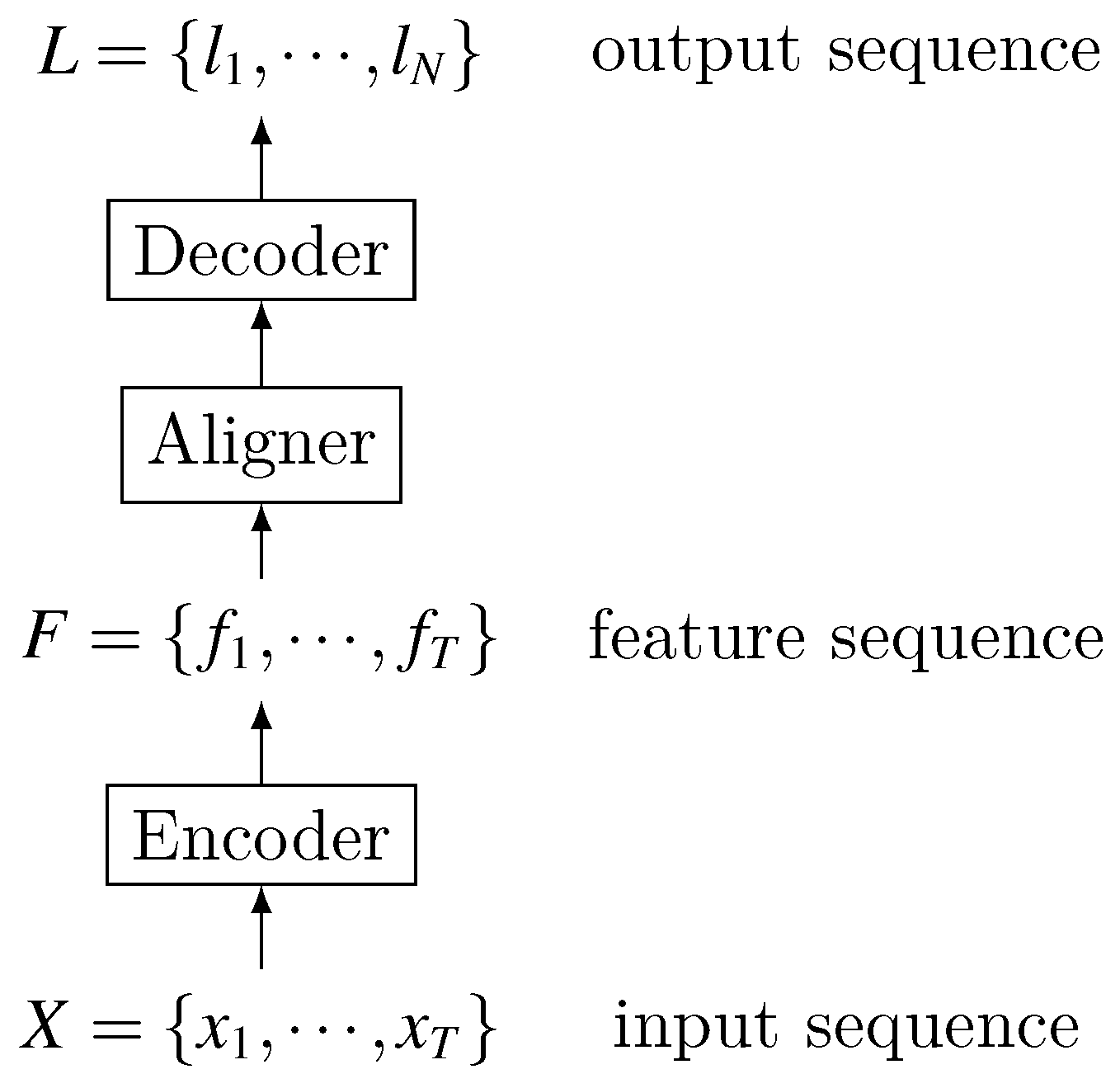
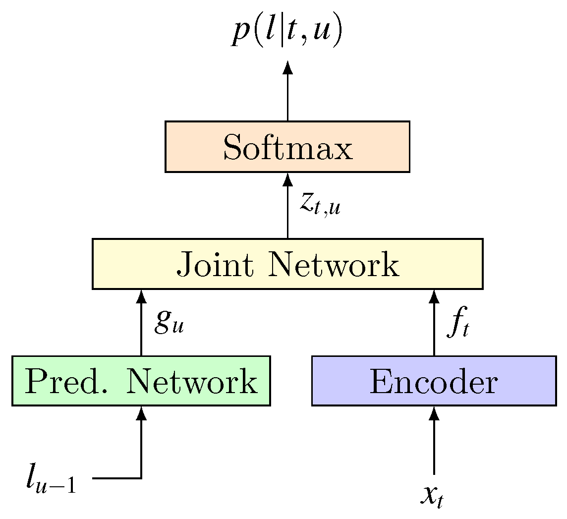
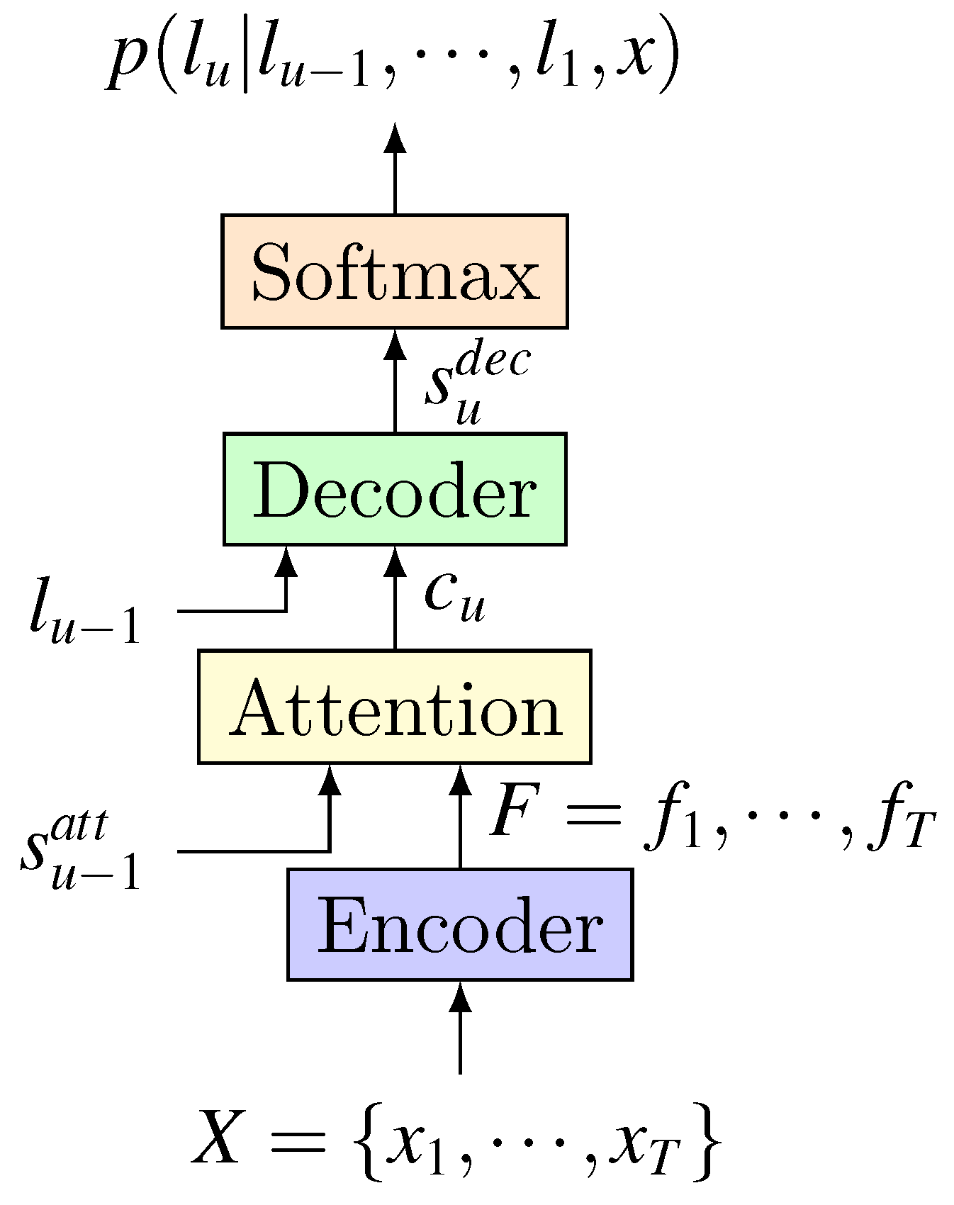
Table 1.
Model characteristics comparison.
| Model | Delay | Computation Complexity | Language Model Ability | Training Difficulty | Recognition Accuracy |
|---|---|---|---|---|---|
| CTC-based | × | ||||
| RNN-Transducer | √ | ||||
| Attention-based | √ |
Table 2.
Model recognition performance comparison [38].
Table 2.
Model recognition performance comparison [38].
| Model | Clean | Noisy | Numeric | ||
|---|---|---|---|---|---|
| Dict | vs | Dict | vs | ||
| Baseline Uni.CDP | 6.4 | 9.9 | 8.7 | 14.6 | 11.4 |
| Baseline BiDi.CDP | 5.4 | 8.6 | 6.9 | - | 11.4 |
| End-to-End systems | |||||
| CTC-Grapheme | 39.4 | 53.4 | - | - | - |
| RNN Transducer | 6.6 | 12.8 | 8.5 | 22.0 | 9.9 |
| RNN Trans.with att. | 6.5 | 12.5 | 8.4 | 21.5 | 9.7 |
| Att. 1-layer dec. | 6.6 | 11.7 | 8.7 | 20.6 | 9.0 |
| Att. 2-layer dec. | 6.3 | 11.2 | 8.1 | 19.7 | 8.7 |
© 2019 by the authors. Licensee MDPI, Basel, Switzerland. This article is an open access article distributed under the terms and conditions of the Creative Commons Attribution (CC BY) license (http://creativecommons.org/licenses/by/4.0/).
Share and Cite
MDPI and ACS Style
Wang, D.; Wang, X.; Lv, S. An Overview of End-to-End Automatic Speech Recognition. Symmetry 2019, 11, 1018. https://0-doi-org.brum.beds.ac.uk/10.3390/sym11081018
AMA Style
Wang D, Wang X, Lv S. An Overview of End-to-End Automatic Speech Recognition. Symmetry. 2019; 11(8):1018. https://0-doi-org.brum.beds.ac.uk/10.3390/sym11081018
Chicago/Turabian StyleWang, Dong, Xiaodong Wang, and Shaohe Lv. 2019. "An Overview of End-to-End Automatic Speech Recognition" Symmetry 11, no. 8: 1018. https://0-doi-org.brum.beds.ac.uk/10.3390/sym11081018
Note that from the first issue of 2016, this journal uses article numbers instead of page numbers. See further details here.