Diffusive and Anti-Diffusive Behavior for Kinetic Models of Opinion Dynamics

Abstract

In the present paper, we study a class of nonlinear integro-differential equations of a kinetic type describing the dynamics of opinion for two types of societies: conformist ($\sigma =1$) and anti-conformist ($\sigma =-1$). The essential role is played by the symmetric nature of interactions. The class may be related to the mesoscopic scale of description. This means that we are going to statistically describe an individual state of an agent of the system. We show that the corresponding equations result at the macroscopic scale in two different pictures: anti-diffusive ($\sigma =1$) and diffusive ($\sigma =-1$). We provide a rigorous result on the convergence. The result captures the macroscopic behavior resulting from the mesoscopic one. In numerical examples, we observe both unipolar and bipolar behavior known in political sciences.

1. Introduction

In Ref. [1] a general model of swarming behavior of an individual population was proposed and studied. The main aim in that paper was to study the macroscopic (so-called “hydrodynamic”) limit. The mathematical structure proposed therein seems very rich and interesting from the mathematical point of view—see the analysis of its simplification in Refs. [2,3,4].

In the present paper, we study the time evolution of the probability density f. The function $f=f(t,u)$ is the distribution of an internal, microscopic state $u\in {\mathbb{R}}^d$ at time $t\ge 0$ of a (statistical or test) agent. Such a description has then a mesoscopic nature. An arbitrary vector $u\in {\mathbb{R}}^d$ can be related to a biological state, activity, opinion (e.g., political opinion), a social state of a test agent, etc.—cf. [1,5,6,7] and references therein, $d=1,2,\dots$. The model has therefore a wide range of possible applications in various applied sciences, such as biology, medicine, social or political sciences.

Because some results of the present paper may have a particular importance in the description in social sciences, we will refer the parameter u to as the opinion of (test) agent.

The time evolution is defined by the general nonlinear integro-differential Boltzmann-like equation, see Ref. [1] and references therein,

$${\partial }_{t}f(t,u)=Q\left[f\right](t,u),u\in {\mathbb{R}}^d,t\ge 0,$$

(1)

where

$$\begin{array}{c}Q\left[f\right](t,u)=\underset{{\mathbb{R}}^d}{\int }\left(T\left[f\right(t,.\left)\right](v,u)f(t,v)-f(t,u)T\left[f\right(t,.\left)\right](u,v)\right)\mathrm{d}v.\hfill \end{array}$$

The nonlinear operator Q describes interactions between agents causing a change of opinion. The turning rate $T\left[f\right](u,v)$ measures the rate for an agent with opinion u to change it into v. A simpler equation, with two possible states only, was studied in Ref. [8]—see also Ref. [6]. It is a typical kinetic (microscopic or more precisely, mesoscopic) way of describing large (social) populations. Instead of dealing with the states of all separated agents involved in the population evolution, we deal with the statistical state of one (test) agent. This state is described by the probability density f that is a solution of Equation (1). The main aim is to describe general dispersion–concentration phenomena resulting from individual opinions of agents. The dispersion results in the presence of various opinions in a society, whereas the concentration represents a kind of uniformity of opinions. The main advantage of the class of models given by Equation (1) is that it can capture many scenarios that are known in social sciences.

There is an increasing interest in a kinetic approach in a similar context. Ref. [9] is dedicated to the modeling and simulation of swarms, where interactions at the microscopic scale are modeled by stochastic games. Ref. [10] describes the state of the art of swarming at the individual–based level and the macroscopic level. Ref. [5] models ensembles of social agents as behavioral, evolutionary, complex systems referring to the complexity features of living systems. Individual–based approaches based on stochastic processes are proposed in Refs. [7,11,12]. Ref. [13] studies the local stability of Dirac masses for a kinetic model of alignment. See also references therein.

The modeling process leads to a proper choice of the turning rate. In the present paper, we are going to study two different and somehow opposite choices.

Case 1.

(A conformist society). Let

$$T\left[f(t,.)\right](u,v)=\beta (u,v)f^{\gamma }(t,v),u,v\in {\mathbb{R}}^d,$$

where $\gamma >1$ is a given number.

Throughout the paper we assume that $\beta$ is a symmetric function of its arguments, i.e.,

$$\beta (u,v)=\beta (v,u)\mathrm{for}\mathrm{all}u,v\in {\mathbb{R}}^d.$$

(2)

This assumption, which may be related to a symmetric nature of interactions between agents, is essential for the mathematical theory presented here. In fact relaxing of the assumption leads to a completely different behavior and different macroscopic limits. In such a case one may expect first order terms that dominate in the macroscopic picture causing a drift towards some states.

The rate of transition from opinion u to opinion v is proportional to $\gamma$-power of the actual probability of having opinion v. The higher the probability, the larger the chance of a change. Therefore it is natural to refer to such a society as a conformist society (or a collectivistic society). The interaction kernel $\beta$ corresponds to the tendency of agents to change opinion. In particular, it may restrict the interactions to close opinions only—see Ref. [4]. The (sensitivity) parameter $\gamma$ describes the level of sensitivity of interactions. The greater $\gamma$, the more sensitive interactions.

The models defined by Case 1 was proposed in Ref. [1], and then studied in various directions in Refs. [2,3,4]. Ref. [1] proposed results of global existence in the space homogeneous case for $0<\gamma <1$, whereas $\gamma >1$ was considered in Ref. [2,3,4]. Assuming that $\gamma =1$ yields a trivial model, thus it is excluded. Alternatively, we may propose:

Case 2.

(A moderately anti-conformist society). Let

$$T\left[f(t,.)\right](u,v)=\beta (u,v)f(t,v)f^{\gamma -1}(t,u),u,v\in {\mathbb{R}}^d,$$

where $\gamma >1$ is a given number.

The rate of transition from opinion u to opinion v is proportional to the product of $\gamma -1$-power of the actual probability of having opinion u and the actual probability of having opinion v. The higher the product, the larger the chance of a change. Therefore, we may refer to such a society as a moderately anti-conformist society (or a individualistic society). As before, the interaction kernel $\beta$ corresponds to the tendency of agents to change opinion.

One may note that the following choice of $T\left[f\right(t,.\left)\right]$ leads to the same kinetic equation, again justifying its name (the moderately anti-conformist society) (or individualistic society).

Case 3.

Let

$$T\left[f(t,.)\right](u,v)=\beta (u,v)f(t,v)\left(M^{\gamma -1}\left(t\right)-f^{\gamma -1}(t,v)\right),u,v\in {\mathbb{R}}^d,$$

where $\gamma >1$ is a given number and $M\left(t\right)=\mathrm{ess}\underset{u\in {\mathbb{R}}^d}{sup}f(t,u)$.

Both Cases 1 and 2 (or 3) can be put together as the following equation

$$\begin{array}{c}{\partial }_{t}f(t,u)=Q\left[f\right](t,u)=\hfill \\ =\sigma \underset{{\mathbb{R}}^d}{\int }\left(\beta (v,u)f(t,v)f^{\gamma }(t,u)-\beta (v,u)f(t,u)f^{\gamma }(t,v)\right)\mathrm{d}v,\hfill \\ u\in {\mathbb{R}}^d,t\ge 0,\hfill \end{array}$$

(3)

where $\sigma =\pm 1$. Condition $\sigma =1$ corresponds to Case 1, whereas $\sigma =-1$ to Case 2 (or Case 3).

The main Equation (3) reads

$${\partial }_{t}f(t,u)=\sigma \left(\left(\beta *f\right)(t,u)f^{\gamma }(t,u)-f(t,u)\left(\beta *f^{\gamma }\right)(t,u)\right)$$

(4)

$u\in {\mathbb{R}}^d$, $t\ge 0$, whereby $\left(\beta *f\right)$ we denote the convolution-like product, i.e.,

$$\left(\beta *f\right)(t,u)=\underset{{\mathbb{R}}^d}{\int }\beta \left(u,v\right)f\left(t,v\right)\mathrm{d}v.$$

The $L^p$-norm is denoted by ${\parallel .\parallel }_p$. We may state the following existence–uniqueness result for solutions to Equation (4).

Proposition 1.

Let $\gamma >1$. If $f_0$ is a probability density such that $f_0\in L^{\infty }\left({\mathbb{R}}^d\right)$, then there exists $T>0$ such that the solution $f=f\left(t\right)$ to (4) exists and is unique in $L^{\infty }\left({\mathbb{R}}^d\right)\cap L^1\left({\mathbb{R}}^d\right)$ on the interval $[0,T)$. The solution preserves the positivity and $L^1$-norm (i.e., it is a probability density) on $[0,T)$. Moreover,

1. 

If $\sigma =-1$ the solution is global and possesses all finite $L^p$-norms, $p>1$, and the functions $t\mapsto {\parallel f\left(t\right)\parallel }_p$ are decreasing;

2. 

If $\sigma =1$ the solution, depending on initial data, is either global ($T=\infty$) or local ($T<\infty$), it possesses all finite $L^p$-norms on $[0,T)$, $p>1$, and the functions $t\mapsto {\parallel f\left(t\right)\parallel }_p$ are increasing for $t\in [0,T)$.

Proof. 

The proof follows from Ref. [1]. First we observe that the operator on the right-hand side of Equation (4) is locally Lipschitz-continuous in the $L^{\infty }\left({\mathbb{R}}^d\right)\cap L^1\left({\mathbb{R}}^d\right)$-setting. Therefore, the existence in this setting on some interval $[0,T)$ follows. It is easy to see that the solution $f=f\left(t\right)$ preserves positivity and $L^1\left({\mathbb{R}}^d\right)$-norm of the initial datum, $t\in [0,T)$.

Let $\lambda \left(x\right)=x^p$, $p>1$. Then the solution $f=f\left(t\right)$ a priori satisfies

$$\begin{array}{c}\frac{\mathrm{d}}{\mathrm{d}t}\underset{{\mathbb{R}}^d}{\int }\lambda \left(f(t,u)\right)\mathrm{d}u=\frac{\sigma }{2}\underset{{\mathbb{R}}^d}{\int }\underset{{\mathbb{R}}^d}{\int }\beta (u,v)f(t,u)f(t,v)\times \hfill \\ \left(f^{\gamma -1}(t,u)-f^{\gamma -1}(t,v)\right)\left({\lambda }^{\prime }\left(f(t,u)\right)-{\lambda }^{\prime }\left(f(t,v)\right)\right)\mathrm{d}v\mathrm{d}u.\hfill \end{array}$$

Therefore, the conclusion follows. □

Moreover, we need the smoothness of the solutions. Let $W^{m,p}\left({\mathbb{R}}^d\right)$ and $C_B^m\left({\mathbb{R}}^d\right)$ be the Banach spaces—the classical Sobolev space (a subspace of $L^p\left({\mathbb{R}}^d\right)$) and the space of m-differentiable functions, respectively, with the usual norms denoted by ${\parallel .\parallel }_p^{\left(m\right)}$ and ${\parallel .\parallel }_{\left[B\right]}^{\left(m\right)}$, respectively.

Let $X^{\left(m\right)}=W^{m,1}\left({\mathbb{R}}^d\right)\cap C_B^m\left({\mathbb{R}}^d\right)$, $m=0,1,2,\dots$, and ${\parallel .\parallel }^{\left(m\right)}$ be defined

$${\parallel .\parallel }^{\left(m\right)}={\parallel .\parallel }_1^{\left(m\right)}+{\parallel .\parallel }_{\left[B\right]}^{\left(m\right)},m=0,1,2,\dots .$$

In particular, for $m=0$, we write $X=X^{\left(0\right)}=L^1\left({\mathbb{R}}^d\right)\cap L^{\infty }\left({\mathbb{R}}^d\right)$ and $\parallel .\parallel ={\parallel .\parallel }^{\left(0\right)}$.

Proposition 2.

Let the assumption of Proposition 1 be satisfied and additionally $f_0\in X^{\left(m\right)}$ and

$$\left(\beta \ast g\right)\in X^{\left(m\right)}\mathrm{for}\mathrm{each}g\in X^{\left(m\right)},$$

(5)

for some $m=1,2,3,\dots$. Then the solution $f=f\left(t\right)$ (given by Proposition 1) satisfies $f(t,.)\in X^{\left(m\right)}$ for all $t\in [0,T)$.

Proof. 

The proof follows again by the standard application of Lipschitz-continuity in $X^{\left(m\right)}$. □

2. Formal Diffusive and Anti-Diffusive Limits

In the present section we study (only in a formal way) the macroscopic limits of Equation (4) with both $\sigma =1$ and $\sigma =-1$. As we will see, the case $\sigma =-1$ corresponds to the diffusive macroscopic behavior, whereas $\sigma =1$—to the anti-diffusive behavior.

Suppose that the support of $\beta$ is concentrated close to the diagonal $\{(u,v)\in {\mathbb{R}}^{2d}:u=v\}$, i.e.,

$$\beta (u,v)=\frac{1}{{\epsilon }^{d+2}{\omega }_d}\chi \left(|u-v|\le \epsilon \right),$$

(6)

where ${\omega }_d$ is the normalizing coefficient, i.e., d-dimensional volume of the unit ball (centered at 0).

We are going to consider $\epsilon \to 0$, because we are interested in the limit as the “support tends to the diagonal” and the non-zero values of $\beta$ tend to infinity. We may note that $\beta$ defined in Equation (6) satisfies Equations (5). The essential role here is again played by the symmetric nature of interactions. Without this nature, the limit could be completely different.

Let the solution of Equation (4), for fixed $\epsilon >0$, be denoted by $f^{\left(\epsilon \right)}=f^{\left(\epsilon \right)}\left(t\right)$ and be in $X^{\left(3\right)}$. If $f^{\left(\epsilon \right)}$ tends to f in $X^{\left(3\right)}$, then f is a solution to the following partial differential equation

$${\partial }_{t}f=\sigma (1-\gamma )\frac{c_d}{2{\omega }_d}\nabla ·\left(f^{\gamma }\nabla f\right)$$

(7)

with the positive constant $c_d$

$$c_d=\underset{\mathbb{B}\left(1\right)}{\int }{\left(v_i\right)}^2\mathrm{d}v,$$

(8)

where $\mathbb{B}\left(1\right)$ is the unit ball. Taking $\gamma >1$ as well as $\sigma =-1$, Equation (7) is the classical porous medium equation—see Refs. [14,15,16] and references therein. On the other hand, taking $\gamma >1$ and $\sigma =1$ we obtain a nonlinear anti-diffusion equation. A linear anti-diffusion equation was also formally obtained as in a hydrodynamic limit in Ref. [8]—see (4.19) and (4.20) therein. Considering regular solutions (i.e., $C^2$ with respect to u), Equation (7) is equivalent to

$${\partial }_{t}f=\frac{\sigma c_d}{2{\omega }_d}\left(f^{\gamma }\Delta f-f\Delta \left(f^{\gamma }\right)\right),$$

(9)

where $\Delta$ is the Laplace operator. We generalize the above argument to Equation (4) with $\beta$ given by

$$\beta (u,v)=\frac{1}{{\epsilon }^{d+2}}\overline{\beta }\left(\frac{u-v}{\epsilon }\right).$$

We do not assume that $\overline{\beta }$ is a probability density but we refer to the notion of generalized moments as well as the generalized covariance matrix in a standard way.

Assumption 1.

We assume

1. 

The function $\overline{\beta }:{\mathbb{R}}^d\to \mathbb{R}$ is bounded, non-negative and symmetric, i.e., $\overline{\beta }\left(v\right)=\overline{\beta }(-v)$;

2. 

The first, second, third, and fourth generalized moments are bounded, i.e.,

$$\underset{{\mathbb{R}}^d}{\int }{\left|v\right|}^p\overline{\beta }\left(v\right)\mathrm{d}v<+\infty \mathrm{for}p=1,2,3,4;$$

3. 

The matrix

$${\Sigma }_{\overline{\beta }}=\left[\underset{{\mathbb{R}}^d}{\int }{v}_i{v}_j\overline{\beta }\left(v\right)\mathrm{d}v\right],$$

the generalized covariance matrix of $\overline{\beta }$, is positive definite.

If $\overline{\beta }$ is a probability density, then the generalized moments and the generalized covariance of $\overline{\beta }$ become just moments and covariance of $\overline{\beta }$. Assumption 1 is satisfied for $\beta$ in Equation (6) if $\overline{\beta }$ is given by

$$\overline{\beta }\left(v\right)=\frac{1}{{\omega }_d}\chi \left(|u-v|\le 1\right).$$

With this $\overline{\beta }$ we put

$$\beta (u,v)=\frac{1}{{\epsilon }^{d+2}}\overline{\beta }\left(\frac{u-v}{\epsilon }\right),$$

(10)

and easily obtain Equation (7), which is formally equivalent to Equation (9). We intend to obtain the following generalization of Equation (9)

$${\partial }_{t}f(t,u)=\frac{\sigma }{2}\left\{f^{\gamma }(t,u){\Sigma }_{\overline{\beta }}·D^{2}f(t,u)-f(t,u){\Sigma }_{\overline{\beta }}·D^2{f}^{\gamma }(t,u)\right\}.$$

(11)

The symbol “·” stands for the inner scalar product of two $d\times d$-matrices and $D^{2}f$ is the Hessian matrix (it consists of second order derivatives in $u_i,u_j$). To obtain Equation (11) we use the Taylor expansions

$$f^{\left(\epsilon \right)}(t,v)=f^{\left(\epsilon \right)}(t,u)+(v-u)·\nabla f^{\left(\epsilon \right)}(t,u)+\frac{1}{2}(v-u)·D^2{f}^{\left(\epsilon \right)}(t,u)(v-u)+\mathcal{O}\left({|v-u|}^3\right),$$

$$\begin{array}{ccc}{\left(f^{\left(\epsilon \right)}\right)}^{\gamma }(t,v)\hfill & =\hfill & {\left(f^{\left(\epsilon \right)}\right)}^{\gamma }(t,u)+(v-u)·\nabla {\left(f^{\left(\epsilon \right)}\right)}^{\gamma }(t,u)\hfill \\ & +\hfill & \frac{1}{2}(v-u)·D^2{\left(f^{\left(\epsilon \right)}\right)}^{\gamma }(t,u)(v-u)+\mathcal{O}\left({|v-u|}^3\right).\hfill \end{array}$$

Substituting these expressions to the right-hand side of Equation (4) and taking into account Equation (10) we obtain

$$\begin{array}{cc}\sigma \hfill & \underset{{\mathbb{R}}^d}{\int }\left(\beta (u,v)f^{\left(\epsilon \right)}(t,v){\left(f^{\left(\epsilon \right)}\right)}^{\gamma }(t,u)-\beta (u,v)f^{\left(\epsilon \right)}(t,u){\left(f^{\left(\epsilon \right)}\right)}^{\gamma }(t,v)\right)\mathrm{d}v\hfill \\ & =\frac{\sigma }{{\epsilon }^{d+2}}\underset{{\mathbb{R}}^d}{\int }\overline{\beta }\left(\frac{u-v}{\epsilon }\right){\left(f^{\left(\epsilon \right)}\right)}^{\gamma }(t,u)(f^{\left(\epsilon \right)}(t,u)+\nabla f^{\left(\epsilon \right)}(t,u)·(v-u)\hfill \\ & +\frac{1}{2}(v-u)·D^2{f}^{\left(\epsilon \right)}(t,u)(v-u)+\mathcal{O}\left({|v-u|}^3\right))\mathrm{d}v\hfill \\ & -\frac{\sigma }{{\epsilon }^{d+2}}\underset{{\mathbb{R}}^d}{\int }\overline{\beta }\left(\frac{u-v}{\epsilon }\right)f^{\left(\epsilon \right)}(t,u)({\left(f^{\left(\epsilon \right)}\right)}^{\gamma }(t,u)+\nabla {\left(f^{\left(\epsilon \right)}\right)}^{\gamma }(t,u)·(v-u)\hfill \\ & +\frac{1}{2}(v-u)·D^2{\left(f^{\left(\epsilon \right)}\right)}^{\gamma }{(t,u)(v-u)+\mathcal{O}\left(\right|v-u|}^3\left)\right)\mathrm{d}v.\hfill \end{array}$$

(12)

From the symmetry of $\overline{\beta }$, the first order terms with respect to $v-u$ vanish. The second order terms yield

$$\frac{\sigma }{2}\left\{{\left(f^{\left(\epsilon \right)}\right)}^{\gamma }(t,u){\Sigma }_{\overline{\beta }}·D^2\left(f^{\left(\epsilon \right)}\right)(t,u)-f^{\left(\epsilon \right)}(t,u){\Sigma }_{\overline{\beta }}·D^2{\left(f^{\left(\epsilon \right)}\right)}^{\gamma }(t,u)\right\}.$$

In the limit $\epsilon \to 0$ we formally obtain the diffusion or anti-diffusion equation Equation (11).

In the particular case of Equation (6), all mixed (generalized) second moments of $\overline{\beta }\left(v\right)=\frac{1}{{\omega }_d}\chi \left(|u-v|\le 1\right)$ are equal to zero. In that case the pure second (generalized) moments, using Equation (8), are as follows

$$\begin{array}{cc}\sigma \underset{{\mathbb{R}}^d}{\int }\hfill & \left(\beta (v,u)f^{\left(\epsilon \right)}(t,v){\left(f^{\left(\epsilon \right)}\right)}^{\gamma }(t,u)-\beta (v,u)f^{\left(\epsilon \right)}(t,u){\left(f^{\left(\epsilon \right)}\right)}^{\gamma }(t,v)\right)\mathrm{d}v\hfill \\ & =\frac{\sigma c_d}{2{\omega }_d}\left({\left(f^{\left(\epsilon \right)}\right)}^{\gamma }(t,u){\nabla }^2{f}^{\left(\epsilon \right)}(t,u)-f^{\left(\epsilon \right)}(t,u){\nabla }^2\left({\left(f^{\left(\epsilon \right)}\right)}^{\gamma }(t,u)\right)\right)+\mathcal{O}\left(\epsilon \right).\hfill \end{array}$$

(13)

In this case, in the limit $\epsilon \to 0$, Equation (4) formally results in the diffusion/anti-diffusion equation Equation (9). Also, formally, Equation (9) turns to be a porous-media equation when $\sigma =-1$. The existence, uniqueness and regularity criteria are formulated in [15]. There is no such result for anti-diffusion equations, in particular for Equation (9) with $\sigma =1$.

3. Convergence Result

In this section, we are going to prove the rigorous convergence result— a diffusive limit for $\sigma =-1$. It is somehow in the spirit of the diffusive limit for a class of bilinear equations studied in Ref. [17]. We assume stronger regularity of the initial datum $f_0$ and obtain the convergence of order ${\epsilon }^2$. Due to the symmetry of $\beta$ one can enhance the convergence rate from ${\epsilon }^1$ to ${\epsilon }^2$.

Concerning Equation (4) with $\sigma =-1$ the global existence and uniqueness follows from Proposition 1, for its diffusive limit (7)—from [15] (by the porous-media theory), whereas the case $\sigma =1$ is almost completely unknown.

We transform Equation (11) to a porous-media equation, for which one can state an existence result in the diffusive case $\sigma =-1$. Since the matrix ${\Sigma }_{\overline{\beta }}$ is symmetric and positive–definite, there is a $d\times d$-matrix B such that ${\Sigma }_{\overline{\beta }}=B^2$. We can now define a new function $F(t,u)=f\left(t,Bu\right)$ and establish the relations between the derivatives

$$\nabla F(t,u)=\left(B\nabla f\right)\left(t,Bu\right)\Delta F(t,u)=\left(B^2·D^{2}f\right)\left(t,Bu\right)=\left({\Sigma }_{\overline{\beta }}·D^{2}f\right)\left(t,Bu\right).$$

(14)

Herewith Equation (11) transforms to

$${\partial }_{t}F=-\frac{1}{2}{F}^{\gamma }\Delta F+\frac{1}{2}F\Delta F^{\gamma }.$$

(15)

The initial condition is given by $F_0\left(u\right)=f_0\left(Bu\right)$. It follows

$$\nabla ·\left(F^{\gamma }\nabla F\right)(t,u)=\nabla ·\left(F^{\gamma }\left(t,u\right)\left(B\nabla f\right)\left(t,Bu\right)\right)=\frac{1}{\gamma +1}{B}^2·D^2\left(f^{\gamma +1}\right)\left(t,Bu\right).$$

(16)

In this way we arrive at an equation which is formally equivalent to Equation (11) and reduces to a porous-media equation

$${\partial }_{t}f=\frac{\gamma -1}{2(\gamma +1)}{\Sigma }_{\overline{\beta }}·D^2\left(f^{\gamma +1}\right).$$

(17)

The respective function $F(t,u)=f(t,Bu)$ satisfies the porous-media equation

$${\partial }_{t}F=\frac{\gamma -1}{2(\gamma +1)}\Delta \left(F^{\gamma +1}\right).$$

(18)

We are ready to formulate an existence result.

Proposition 3.

Let $\gamma >1$, $\sigma =-1$ and $f_0$ be a probability density on ${\mathbb{R}}^d$ such that $f_0\in X^{\left(p\right)}$. Let moreover $\overline{\beta }\in X$ satisfy Assumption 1. Then Equation (17) with the initial condition $f\left(0\right)=f_0$ has a unique solution $f=f\left(t\right)$ in $X^{\left(p\right)}$, on some interval $[0,T]$.

Proof. 

By the substitution $F(t,u)=f\left(t,Bu\right)$ Equations (17) reduces to (18), in other words

$${\partial }_{t}F=\frac{\gamma -1}{2}\nabla ·\left(F^{\gamma }\nabla F\right)$$

with the initial condition $F_0\left(u\right)=f_0\left(Bu\right)$. The assertion follows from the porous-media existence theory. □

Theorem 1.

Let $\gamma >1$, $\sigma =-1$ as well as $f_0$ be a probability density on ${\mathbb{R}}^d$ such that $f_0\in X^{\left(4\right)}$. Let moreover $\overline{\beta }\in X$ be a non-negative function satisfying Assumption 1 and let $f^{\left(\epsilon \right)}=f^{\left(\epsilon \right)}\left(t\right)$ defined on $[0,T]\times {\mathbb{R}}^d$ be a solution of Equation (4) with the initial datum $f_0$ and with

$$\beta (u,v)=\frac{1}{{\epsilon }^{d+2}}\overline{\beta }\left(\frac{u-v}{\epsilon }\right).$$

If $f=f\left(t\right)$ in X is a solution to Equation (17) with the same initial datum $f_0$, then

$$\underset{[0,T]}{sup}\parallel f^{\left(\epsilon \right)}-f\parallel \le C{\epsilon }^2$$

with some constant $C>0$.

Proof. 

Let $f^{\left(\epsilon \right)}\in X^{\left(4\right)}$ be the solution to Equation (4) with $\beta$ defined by (10). The idea of the proof is as follows:

• the kinetic equation is transformed into an equation formally equivalent to a porous-media equation with a small perturbation;
• the perturbed porous-media equation is reduced to its standard form by the change of variables $u\to Bu$;
• the comparison principle for porous-media equations is applied.

We fix $(t,u)\in [0,T]\times {\mathbb{R}}^d$. Using the Taylor expansions to Equation (4) as in Section 2, we obtain the right-hand side given by Equation (12). From the symmetry of $\overline{\beta }$, the first and third order terms with respect to $v-u$ vanish. The second order terms yield

$$\begin{array}{ccc}\hfill I_{\epsilon }\left(f^{\left(\epsilon \right)}\right)(t,u)& =& \frac{-1}{2}\left\{{\left(f^{\left(\epsilon \right)}\right)}^{\gamma }(t,u){\Sigma }_{\overline{\beta }}·D^2\left(f^{\left(\epsilon \right)}\right)(t,u)-f^{\left(\epsilon \right)}(t,u){\Sigma }_{\overline{\beta }}·D^2{\left(f^{\left(\epsilon \right)}\right)}^{\gamma }(t,u)\right\}\hfill \\ & =& \frac{\gamma -1}{2(\gamma +1)}{\Sigma }_{\overline{\beta }}·\left(D^2{f}^{\gamma +1}\right).\hfill \end{array}$$

Hence Equation (12) reads

$$\begin{array}{cc}\underset{{\mathbb{R}}^d}{\int }\hfill & \frac{1}{{\epsilon }^{d+2}}\overline{\beta }\left(\frac{u-v}{\epsilon }\right)\left(f^{\left(\epsilon \right)}(t,v){\left(f^{\left(\epsilon \right)}\right)}^{\gamma }(t,u)-f^{\left(\epsilon \right)}(t,u){\left(f^{\left(\epsilon \right)}\right)}^{\gamma }(t,v)\right)\mathrm{d}v\hfill \\ & =I_{\epsilon }\left(f^{\left(\epsilon \right)}\right)(t,u)+R_{\epsilon }\left(f^{\left(\epsilon \right)}\right)(t,u),\hfill \end{array}$$

where

$$\begin{array}{ccc}{R}_{\epsilon }\left(f^{\left(\epsilon \right)}\right)(t,u)\hfill & =\hfill & \underset{{\mathbb{R}}^d}{\int }\frac{1}{{\epsilon }^{d+2}}\overline{\beta }\left(\frac{u-v}{\epsilon }\right){\left(f^{\left(\epsilon \right)}\right)}^{\gamma }(t,u)\underset{0}{\overset{1}{\int }}\frac{{(1-\theta )}^3}{6}{D}^4{f}^{\left(\epsilon \right)}(t,u+\theta (v-u)){(v-u)}^4\mathrm{d}\theta \mathrm{d}v\hfill \\ & +\hfill & \underset{{\mathbb{R}}^d}{\int }\frac{1}{{\epsilon }^{d+2}}\overline{\beta }\left(\frac{u-v}{\epsilon }\right)f^{\left(\epsilon \right)}(t,u)\underset{0}{\overset{1}{\int }}\frac{{(1-\theta )}^3}{6}{D}^4{\left(f^{\left(\epsilon \right)}\right)}^{\gamma }(t,u+\theta (v-u)){(v-u)}^4\mathrm{d}\theta \mathrm{d}v,\hfill \end{array}$$

where $D^4{\left(f^{\left(\epsilon \right)}\right)}^p$ consists of all fourth-order partial derivatives ${\partial }_{u_i{u}_j{u}_k{u}_l}^4{\left(f^{\left(\epsilon \right)}\right)}^p$ and $D^4{\left(f^{\left(\epsilon \right)}\right)}^p(t,u+\theta (v-u)){(v-u)}^4$ is the 4-linear form $D^4{\left(f^{\left(\epsilon \right)}\right)}^p(t,u+\theta (v-u))$ acting on four copies of the vector $v-u$. The remainder $R_{\epsilon }\left(f^{\left(\epsilon \right)}\right)$ can be estimated by

$$\underset{{\mathbb{R}}^d}{\int }\frac{1}{{\epsilon }^{d+2}}\overline{\beta }\left(\frac{u-v}{\epsilon }\right)f^{\left(\epsilon \right)}(t,u){|v-u|}^4\underset{0}{\overset{1}{\int }}\frac{{(1-\theta )}^3}{6}\left(\parallel f^{\left(\epsilon \right)}{\parallel }_{L^{\infty }}^{\gamma -1}\parallel D^4{f}^{\left(\epsilon \right)}{\parallel }_{L^{\infty }}+{\parallel D^4{\left(f^{\left(\epsilon \right)}\right)}^{\gamma }\parallel }_{L^{\infty }}\right)\mathrm{d}\theta \mathrm{d}v,$$

and the X-norm can be estimated by $C{\epsilon }^2$ where C is a constant depending on the fourth moments of $\overline{\beta }$ and the $L^{\infty }$-norm of $D^4{f}^{\left(\epsilon \right)}$.

Finally, we attempt to a comparison of $f^{\left(\epsilon \right)}$ with f. The above consideration leads to a perturbed porous-media equation for $f^{\left(\epsilon \right)}$

$${\partial }_t{f}^{\left(\epsilon \right)}(t,u)=\frac{\gamma -1}{2(\gamma +1)}{\Sigma }_{\overline{\beta }}·D^2{\left(f^{\left(\epsilon \right)}\right)}^{\gamma +1}+R_{\epsilon }\left(f^{\left(\epsilon \right)}\right)(t,u).$$

Alike the transformation $f\to F$, one can define $F^{\left(\epsilon \right)}(t,u):=f^{\left(\epsilon \right)}\left(t,Bu\right)$, which satisfies

$${\partial }_t{F}^{\left(\epsilon \right)}(t,u)=\frac{\gamma -1}{2(\gamma +1)}\Delta {\left(f^{\left(\epsilon \right)}\right)}^{\gamma +1}+R_{\epsilon }\left(f^{\left(\epsilon \right)}\right)(t,Bu)$$

with the initial condition $F^{\left(\epsilon \right)}(0,u)=F_0\left(u\right)=f_0\left(Bu\right)$. Since F satisfies the porous-media Equation (18) with the same initial datum, one can apply classical comparison theorems for porous media, see [18,19]. This leads to the estimate

$$\underset{[0,T]}{sup}\parallel F^{\left(\epsilon \right)}-F\parallel \le C{\epsilon }^2.$$

Since the matrix B is non-singular, we obtain a similar estimate for $f^{\left(\epsilon \right)}-f$. This completes the proof. □

If mixed moments (or mixed generalized moments) of $\overline{\beta }$ vanish, the covariance matrix ${\Sigma }_{\overline{\beta }}$ is a diagonal matrix. Therefore, the diffusive/anti-diffusive limit equation, i.e., Equation (9), is a particular case of Equation (11). This fact in the case $\sigma =-1$ we state in the following:

Corollary 1.

Let $\gamma >1$, $\sigma =-1$ as well as $f_0$ be a probability density on ${\mathbb{R}}^d$ such that $f_0\in X^{\left(4\right)}$. Let $f^{\left(\epsilon \right)}=f^{\left(\epsilon \right)}\left(t\right)$ defined on $[0,T]\times {\mathbb{R}}^d$ be solutions of Equation (4) with the initial datum $f_0$ and with β given by (6). If $f=f\left(t\right)$ in X, $t\in [0,T]$, is a solution to Equation (7) with the same initial datum, on $[0,T]\times {\mathbb{R}}^d$, then

$$\underset{[0,T]}{sup}\parallel f^{\left(\epsilon \right)}-f\parallel \le C{\epsilon }^2$$

with some constant $C>0$.

Proof. 

It is sufficient to put $\overline{\beta }\left(v\right)=\frac{1}{{\omega }_d}\chi \left(\left|v\right|\le 1\right)$. This is a probability density. Then the covariance matrix ${\Sigma }_{\overline{\beta }}$ is proportional to the identity matrix I and the matrix operation ${\Sigma }_{\overline{\beta }}·D^{2}f$ provides $\frac{c_d}{{\omega }_d}\Delta f$. It is seen that Equation (7) is a particular case of Equation (17). □

4. Numerical Examples

The properties of the solutions to the considered equations can be illustrated by some numerical examples. Take $d=1$, $\gamma >1$ and $\sigma =\pm 1$. Since Equation (7) is a limit equation for Equation (4), one can apply some numerical methods such as the finite differences or the method of lines

$$\begin{array}{ccc}\hfill {\partial }_{t}f(t,u)& =& \frac{\sigma }{6}\left(f^{\gamma }(t,u)\frac{f(t,u+\epsilon )-2f(t,u)+f(t,u-\epsilon ))}{{\epsilon }^2}-f(t,u)\frac{f^{\gamma }(t,u+\epsilon )-2f^{\gamma }(t,u)+f^{\gamma }(t,u-\epsilon ))}{{\epsilon }^2}\right)\hfill \end{array}$$

(19)

with $\epsilon >0$. As a matter of fact, this is a continuous version of the method of lines. For $\sigma =-1$ this is an approximation of a porous-media PDE, which is a parabolic equation. One can investigate the convergence.

If we rearrange Equation (19), it turns out that it coincides with an agent-based model corresponding to kinetic equations

$${\partial }_{t}f(t,u)=\frac{\sigma }{6}\left(f^{\gamma }(t,u)\frac{f(t,u+\epsilon )+f(t,u-\epsilon ))}{{\epsilon }^2}-f(t,u)\frac{f^{\gamma }(t,u+\epsilon )+f^{\gamma }(t,u-\epsilon ))}{{\epsilon }^2}\right).$$

(20)

One can see that the solutions to (20) preserve non-negativity of the initial datum as well as $L^1$-norm. In both cases $\sigma =-1$ and $\sigma =1$ one can pass to the limit with $\epsilon \to 0$. Its derivation resembles the diffusive limit for (4).

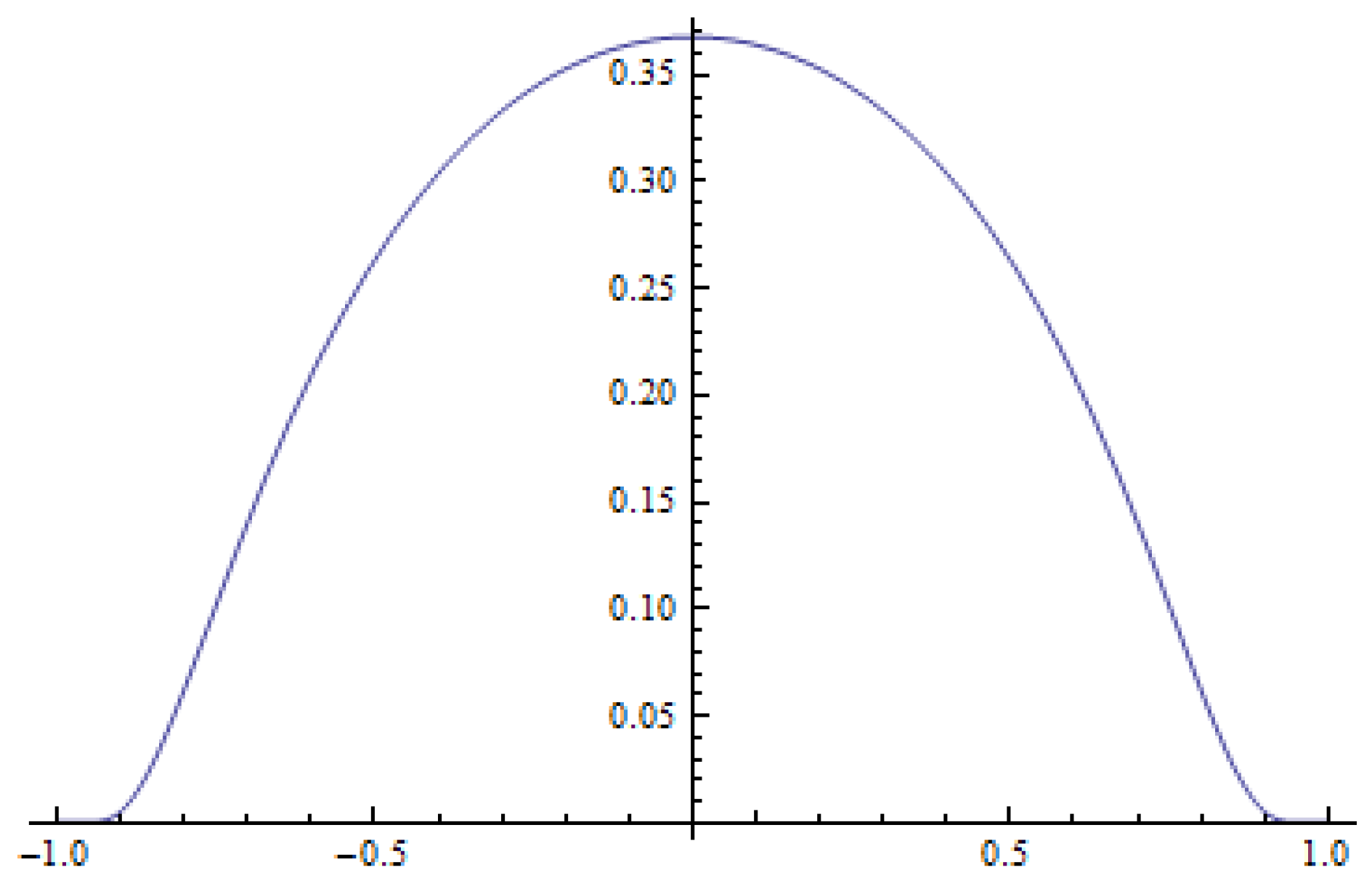
Example 1.

We consider the initial datum in the form

$$f_0\left(u\right)=\left\{\begin{array}{cc}\hfill Cexp(-\frac{1}{1-u^2}),& u\in (-1,1)\hfill \\ \hfill 0,& u\notin (-1,1)\hfill \end{array}\right.,$$

where $C>0$ is a normalizing coefficient. The initial datum $f_0\in X$ is an even function and has a single global maximum at $u=0$ (see Figure 1). Then the solution to the method of lines (19) has unique global maximum at zero.

Please note that

$$f(t,u)\approx f_0\left(u\right)+t{\partial }_{t}f(t,u){|}_{t=0}.$$

(21)

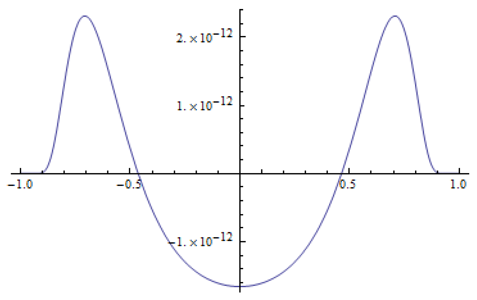
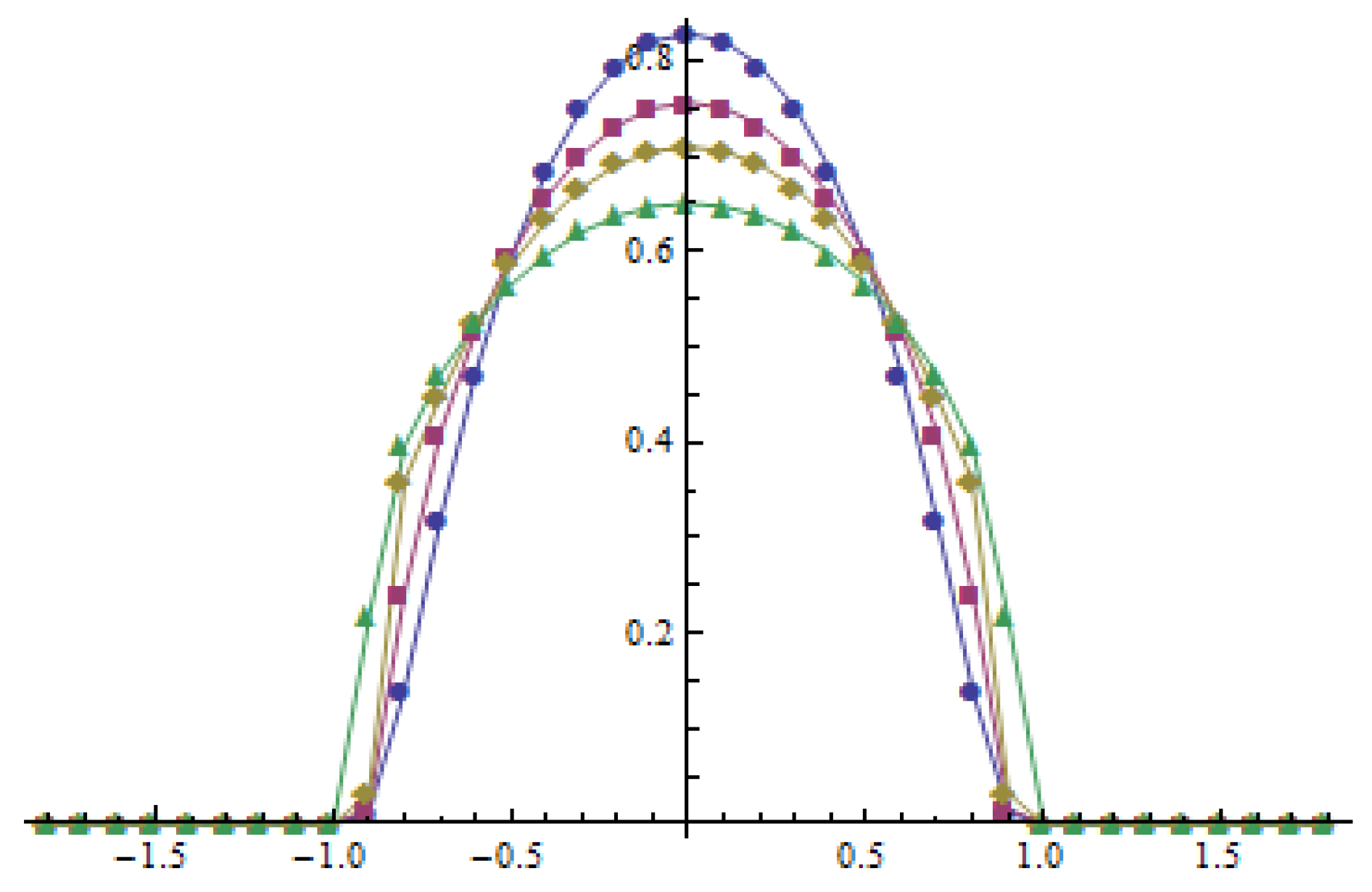
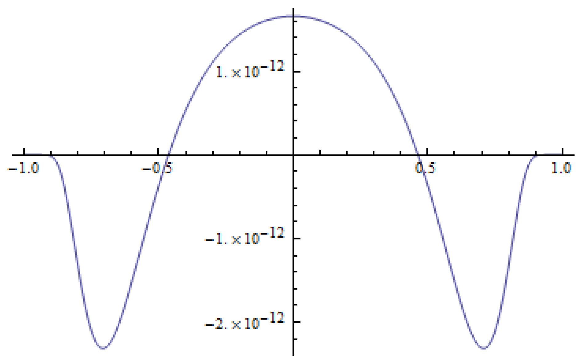
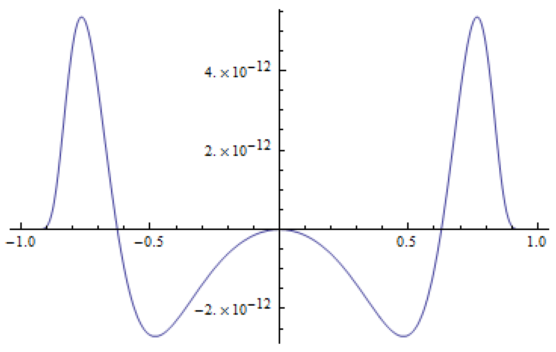
If the time derivative is negative in a neighborhood of zero and $t>0$ (see Figure 2), then the maximum of the initial function is transformed into a smaller value (see Figure 3). Therefore, the solution to (19) with $\sigma =-1$ is dispersive. Otherwise, the maximum of the solution to (19) is increasing ($\sigma =1$, see Figure 4 and Figure 5), and the solutions are not dispersive. The time derivative of the solution for $t=0$ does not have any positive twin peaks in the neighborhood of $u=0$ (see Figure 4), which indicates that the solution for anti-diffusion is unipolar. This follows from the fact that the initial datum and its derivatives satisfy the conditions given in [4] (cf. Theorem 3.1).

Consider $\sigma =\pm 1$. It follows from Proposition 1 that for $\sigma =-1$ the $L^1$-norm and non-negativity of the solution are preserved. The same properties remain for $\sigma =1$. The method of lines for $\sigma =-1$ is stable, unlike for $\sigma =1$. The evolution of the solution is presented at Figure 3 and Figure 5.

Example 2.

We consider the following initial datum

$$f_0\left(u\right)=\left\{\begin{array}{cc}\hfill C(1+u^2)exp(-\frac{1}{1-u^2}),& u\in (-1,1)\hfill \\ \hfill 0,& u\notin (-1,1)\hfill \end{array}\right.,$$

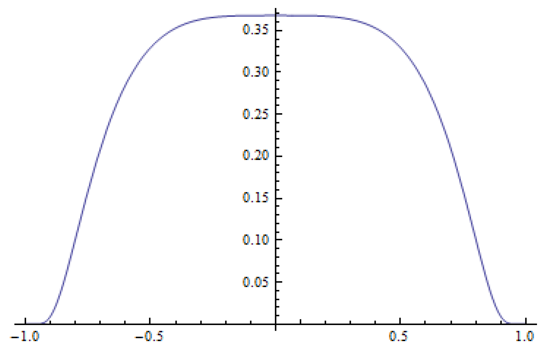
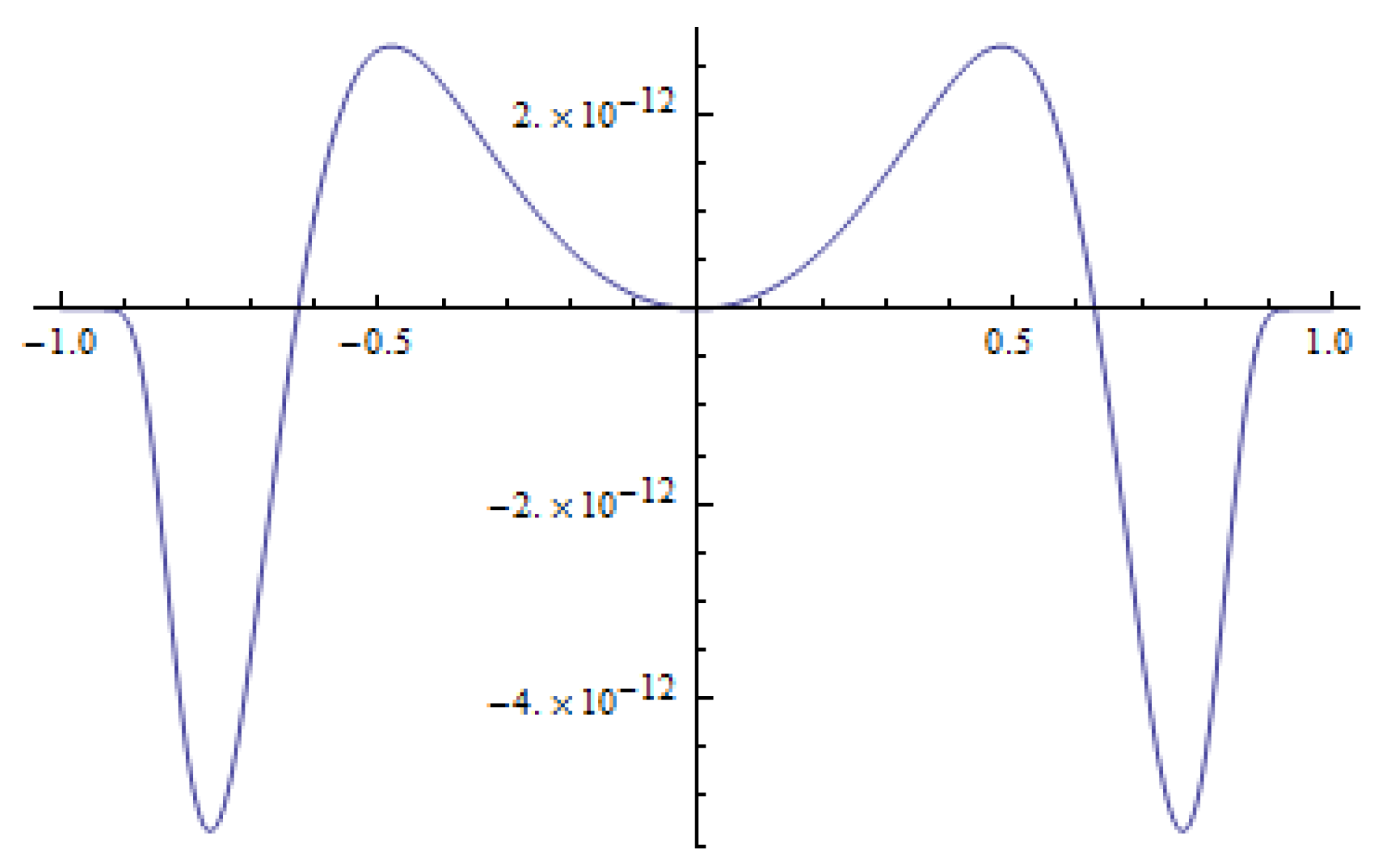
where $C>0$ is the normalizing coefficient. The initial datum has a single peak in the middle of the interval (see Figure 6), moreover, which has the second order derivative that is equal to zero in $u=0$ (see Figure 7). Therefore, the initial datum is “weakly” concave. The behavior of $f_0$ and its second order derivative is presented in Figure 6 and Figure 7. One can see that the initial datum satisfies conditions given in [4] (see Theorem 3.1). Therefore, the method of lines for anti-diffusion transforms the unipolar initial function into the bipolar solution with twin peaks which move away from zero.

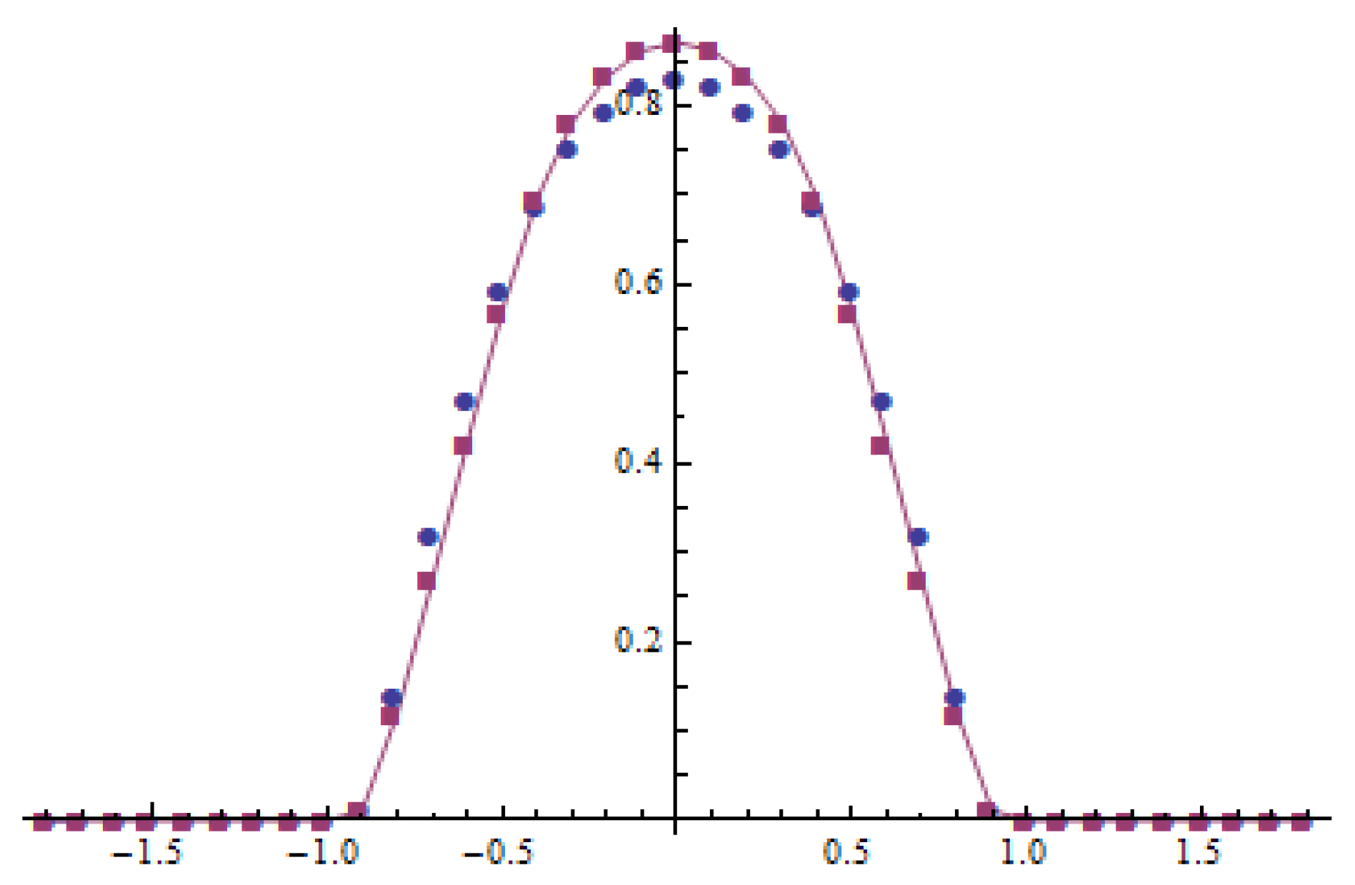
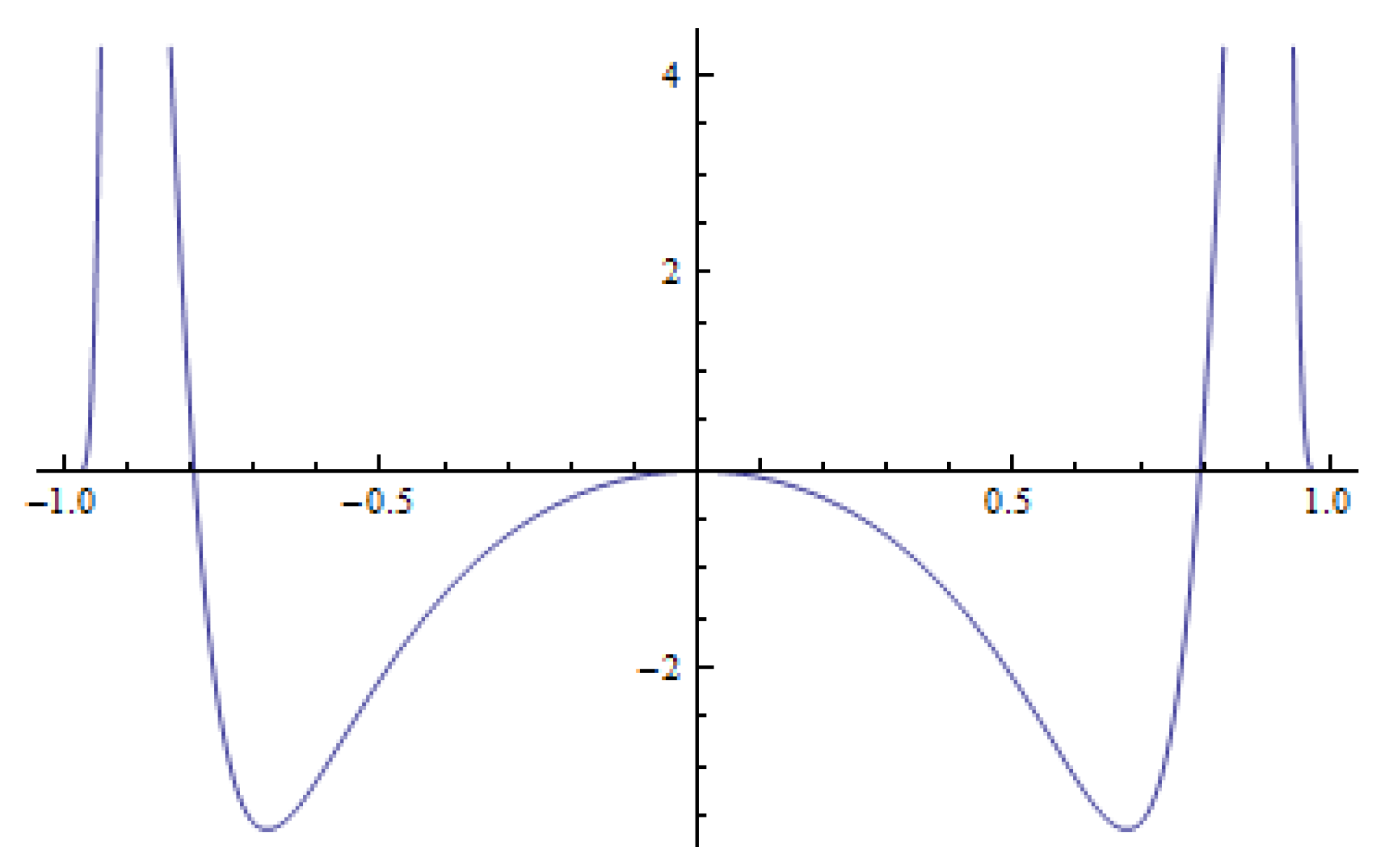
The bipolarity can also be observed in the context of the time derivative for the initial function. The initial function in “weakly” concave in $u=0$. The time derivative for $\sigma =1$ and $t=0$ has symmetric positive twin peaks (see Figure 8). Using the formula (21) one can observe that the values of the time derivative given in the twin peaks added to the values of the initial function in the same points are significantly increasing the value of the initial function. Therefore, the bipolar behavior is observed (see Figure 9).

Considering $\sigma =-1$, the time derivative is presented in Figure 10, and the dispersive evolution is shown in Figure 11.

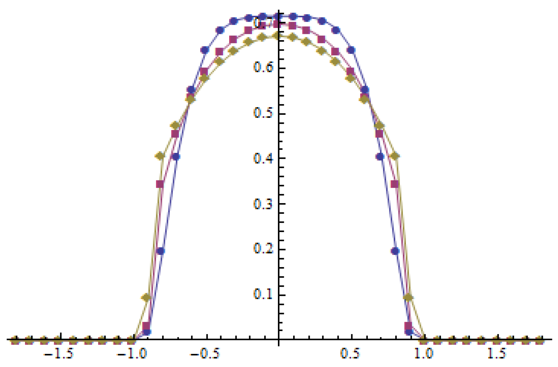
As before, for $\sigma =-1$, the $L^1$-norm and non-negativity of the solution are preserved. The same properties remain for $\sigma =1$. The method of lines for $\sigma =-1$ is stable, unlike for $\sigma =1$. The evolution of the solution to the method of lines for $\sigma =\mp 1$ is presented in Figure 9 and Figure 11.

Our numerical experiments with the method of lines applied to kinetic models in social sciences indicate the possibility of a reliable approximation of short-range interaction opinions in the case of non-conformist societies ($\sigma =-1$). It has a natural interpretation that the model with short interactions is replaced by a discrete model with discrete opinions influencing neighboring opinions. This replacement is constrained by appropriate scaling according to diffusive limits. Concerning the conformist society case ($\sigma =1$), our numerical simulations show numerical instability. However, we observed the unipolar and bipolar phenomenon on a very small time interval.

5. Conclusions

In the paper we studied a class of nonlinear integro-differential kinetic equations that can describe the opinion dynamics for two types of societies— the conformist $\sigma =1$ and anti-conformist $\sigma =-1$. An anti-diffusive (concentration) and a diffusive (dispersive) macroscopic pictures were observed, respectively.

The solutions to the kinetic Equation (4) are a priori positive and preserve $L^1$-norm in both considered cases. For $\sigma =-1$ the existence result is global, whereas for $\sigma =1$ it is only local (see Proposition 1), which can be related to a strong concentration (self-organization) in the latter case.

Assuming that $\beta$ (given by (6)) belongs to $L^1\cap L^{\infty }$, $\sigma =\pm 1$, $\gamma >1$, we conclude that the solutions to the kinetic equation are convergent in X to the solution of a diffusion or (formally) anti-diffusion equations.

In Ref. [4] some bipolar phenomena are described for the kinetic Equation (4). It is a very well-known phenomenon in political sciences (see [4] and references therein).

The present paper opens new interesting problems related to the description of concentration-dispersive phenomena on the mesoscopic scale that may be related to various processes observed in life and social sciences.

References

- Parisot, M.; Lachowicz, M. A kinetic model for the formation of swarms with nonlinear interactions. Kinet. Relat. Model. 2016, 9, 131–164. [Google Scholar] [CrossRef]
- Lachowicz, M.; Leszczyński, H.; Parisot, M. A simple kinetic equation of swarm formation: Blow–up and global existence. Appl. Math. Lett. 2016, 57, 104–107. [Google Scholar] [CrossRef]
- Lachowicz, M.; Leszczyński, H.; Parisot, M. Blow–up and global existence for a kinetic equation of swarm formation. Math. Model. Methods Appl. Sci. 2017, 27, 1153–1175. [Google Scholar] [CrossRef]
- Lachowicz, M.; Leszczyński, H.; Topolski, K.A. Self–organization with small range interactions: Equilibria and creation of bipolarity. Appl. Math. Comput. 2019, 343, 156–166. [Google Scholar] [CrossRef]
- Marsan, G.A.; Bellomo, N.; Gibelli, L. Stochastic evolutionary differential games toward a system theory of behavioral social dynamics. Math. Model. Methods Appl. Sci. 2016, 26, 1051–1093. [Google Scholar] [CrossRef]
- Banasiak, J.; Lachowicz, M. Methods of Small Parameter in Mathematical Biology; Birkhäuser: Boston, MA, USA, 2014. [Google Scholar]
- Lachowicz, M. Individually–based Markov processes modeling nonlinear systems in mathematical biology. Nonlinear Anal. Real World Appl. 2011, 12, 2396–2407. [Google Scholar] [CrossRef]
- Banasiak, J.; Lachowicz, M. On a macroscopic limit of a kinetic model of alignment. Math. Model. Methods Appl. Sci. 2013, 23, 2647–2670. [Google Scholar] [CrossRef]
- Bellomo, N.; Soler, J. On the mathematical theory of the dynamics of swarms viewed as complex systems. Math. Model. Methods Appl. Sci. 2012, 22, 1140006. [Google Scholar] [CrossRef]
- Carrillo, J.A.; Fornasier, M.; Toscani, G.; Vecil, F. Particle, Kinetic, and Hydrodynamic Models of Swarming. In Mathematical Modeling of Collective Behavior in Socio–Economic and Life Sciences; Naldi, G., Pareschi, L., Toscani, G., Eds.; Birkhäuser: Boston, MA, USA, 2010; pp. 297–336. [Google Scholar]
- Carrillo, J.A.; D’Orsogna, M.R.; Panferov, V. Double milling in self–propelled swarms from kinetic theory. Kinet. Relat. Model. 2009, 2, 363–378. [Google Scholar] [CrossRef]
- Carlen, E.; Degond, P.; Wennberg, B. Kinetic limits for pair–interaction driven master equation and biological swarm models. Math. Model. Methods Appl. Sci. 2013, 23, 1339–1376. [Google Scholar] [CrossRef]
- Degond, P.; Frouvelle, A.; Raoul, G. Local stability of perfect alignment for a spatially homogeneous kinetic model. J. Stat. Phys. 2014, 157, 84–112. [Google Scholar] [CrossRef]
- Aronson, D.G. The porous medium equation. In Nonlinear Diffusion Problems; Fasano, A., Primicerio, M., Eds.; Lecture Notes in Mathematics; Springer: Berlin/Heidelberg, Germany, 1986; Volume 1224, pp. 1–46. [Google Scholar]
- Vázquez, J.J. The Porous Medium Equation: Mathematical Theory; Oxford University Press: Oxford, UK, 2007. [Google Scholar]
- Bénilan, P.; Crandall, M.G.; Pierre, M. Solutions of porous medium equation in under optimal conditions on initial values. Indiana Univ. Math. J. 1984, 33, 51–87. [Google Scholar] [CrossRef]
- Lachowicz, M.; Wrzosek, D. Nonlocal bilinear equations: Equilibrium solutions and diffusive limit. Math. Model. Methods Appl. Sci. 2001, 11, 1393–1409. [Google Scholar] [CrossRef]
- Benilan, P.; Brezis, H.; Crandall, M.G. A semilinear equation in L1(). Ann. Scuola Norm. Sup. Pisa 1975, 2, 523–555. [Google Scholar]
- Barbu, V. Nonlinear Semigroups and Differential Equations in Banach Spaces; Noordhoff: Leyden, IL, USA, 1976. [Google Scholar]
Figure 1.
Initial function for .
Figure 2.
Time derivative for , with for .
Figure 3.
Method of lines for , , ; (blue), (red), (yellow), (green).
Figure 4.
Figure 5.
Method of lines for , , ; (blue), (red).
Figure 6.
Figure 7.
Derivative for for .
Figure 8.
Derivative for , with for .
Figure 9.
Method of lines for , , ; (blue), (red), (yellow).
Figure 10.
Figure 11.
© 2019 by the authors. Licensee MDPI, Basel, Switzerland. This article is an open access article distributed under the terms and conditions of the Creative Commons Attribution (CC BY) license (http://creativecommons.org/licenses/by/4.0/).
Share and Cite
MDPI and ACS Style
Lachowicz, M.; Leszczyński, H.; Puźniakowska–Gałuch, E. Diffusive and Anti-Diffusive Behavior for Kinetic Models of Opinion Dynamics. Symmetry 2019, 11, 1024. https://0-doi-org.brum.beds.ac.uk/10.3390/sym11081024
AMA Style
Lachowicz M, Leszczyński H, Puźniakowska–Gałuch E. Diffusive and Anti-Diffusive Behavior for Kinetic Models of Opinion Dynamics. Symmetry. 2019; 11(8):1024. https://0-doi-org.brum.beds.ac.uk/10.3390/sym11081024
Chicago/Turabian StyleLachowicz, Mirosław, Henryk Leszczyński, and Elżbieta Puźniakowska–Gałuch. 2019. "Diffusive and Anti-Diffusive Behavior for Kinetic Models of Opinion Dynamics" Symmetry 11, no. 8: 1024. https://0-doi-org.brum.beds.ac.uk/10.3390/sym11081024
Note that from the first issue of 2016, this journal uses article numbers instead of page numbers. See further details here.