A Comparative Study of Infill Sampling Criteria for Computationally Expensive Constrained Optimization Problems

Abstract

Engineering optimization problems often involve computationally expensive black-box simulations of underlying physical phenomena. This paper compares the performance of four constrained optimization algorithms relying on a Gaussian process model and an infill sampling criterion under the framework of Bayesian optimization. The four infill sampling criteria include expected feasible improvement (EFI), constrained expected improvement (CEI), stepwise uncertainty reduction (SUR), and augmented Lagrangian (AL). Numerical tests were rigorously performed on a benchmark set consisting of nine constrained optimization problems with features commonly found in engineering, as well as a constrained structural engineering design optimization problem. Based upon several measures including statistical analysis, our results suggest that, overall, the EFI and CEI algorithms are significantly more efficient and robust than the other two methods, in the sense of providing the most improvement within a very limited number of objective and constraint function evaluations, and also in the number of trials for which a feasible solution could be located.

1. Introduction

Nature-inspired optimization algorithms, such as swarm intelligence metaheuristics and evolutionary algorithms, have become increasingly popular in recent years for solving optimization problems in different domains, including, for instance, the firefly algorithm [1,2], crow search algorithm [3], hybrid gray wolf optimizer–crow search algorithm [4], elephant herding optimization and tree growth algorithm [5], to name a few. The interested reader is encouraged to consult also [6,7,8,9,10,11] for recent works and applications of nature-inspired algorithms.

When the objective function is computationally expensive (taking a long time to evaluate) and black-box (neither the function expression nor its derivative function are explicitly known), Bayesian optimization (BO) is often employed. Relying on the expected improvement criterion, BO was first proposed by Mockus [12,13] and was popularized by Jones et al. when the framework called the Efficient Global Optimization (EGO) algorithm was introduced [14]. Due to the ease of use and flexibility, the algorithm has been applied to solve different optimization problems in numerous research areas [15,16,17,18,19]. Several modifications to the original EGO developed particularly for unconstrained problems have also been proposed in many works ever since [20,21,22,23,24,25].

Though not as widely used, Bayesian optimization has also been applied to solving constrained optimization problems over the past decade. We now briefly summarize past research on constrained Bayesian optimization (CBO). The method considered in [26] combines the generalized expected improvement criterion with the probability of feasibility, while the expected feasible improvement criterion of [27] combines the expected improvement with constraint functions. Good results were obtained both for simulated and real-world data of learning tasks based on locality sensitive hashing (LSH) hyperparameter tuning and support vector machine (SVM) model compression. The super-efficient global optimization proposed in [28] also includes a feasibility criterion that prevents one from selecting from an infeasible region. Priem et al. [29] proposed a method that uses the the confidence bound [30] to improve the feasibility criterion for better exploring feasible regions in high-uncertainty regions.

Gramacy and Lee proposed a method called integrated expected conditional improvement [31]. The method learns both the objective function and constraint functions at the same time by incorporating a constraint violation into the expected improvement criterion. It sequentially chooses a point whose expected reduction of expected improvement is below the current best observed value and satisfies the constraints. Gelbart et al. [32] studied a criterion for constrained Bayesian optimization problems when noise may be present in the constraint functions and proposed a two-step approach for optimization when the objective and the constraints may be evaluated independently. The next point is selected by maximizing the expected feasible improvement. Then, either the objective or the constraint function will be chosen to evaluate based on the information gain metric. Hernández-Lobato et al. [33] proposed a method called predictive entropy search with constraints, which is an extension of the predictive entropy search [34]. It uses the information gain as a criterion to solve constrained optimization problems and does not require any feasible observation to initialize the algorithm. The rollout algorithm, an adaptation of the method often used in dynamic programming, sequentially selects the next points by maximizing the long-term feasible reduction of the objective function [35]. Numerical results illuminated advantages of the algorithm especially when the objective function is multimodal and the feasible region has a complex topology.

Ariafar et al. [36] proposed an approach that is based on the alternating direction method of multipliers. The method is separated into two solvable problems: the one that minimizes the objective function with a penalty term involving the solution being close to feasible regions and the other that minimizes penalized feasibility over an auxiliary variable that is closest to the solution found in the first step. Recently, Jiao et al. proposed a new sampling criterion for solving optimization problems with constraint functions [37]. The new sampling criterion, called the constrained expected improvement, addressed the issue that the previous expected improvement criterion fails to work because the initial observations do not contain any feasible solutions. The results showed that the algorithm could exploit feasible regions locally as well as explore infeasible yet promising regions efficiently.

From another perspective, an optimization strategy based on stepwise uncertainty reduction principles was proposed for solving a multi-objective optimization [38]. The strategy relies on a sequential reduction of the volume of the excursion sets below the current best solution. Using the same principle, a sampling criterion for a single objective optimization with constraint functions was introduced in [39]. A combination of Gaussian process modeling and the augmented Lagrangian for Bayesian optimization with constraints was proposed by Gramacy et al. [40]. Analytical formulas of the main criterion of the single expensive constraint and the cheap-to-evaluate objective function were subsequently derived in [41], leading to a more efficient implementation of the infill sampling criterion for optimization framework.

Apparently, over the past decade, several Gaussian process (GP)-based infill sampling criteria have been developed and independently tested; however, none of these criteria were rigorously compared under the same umbrella and, in particular, under the BO setting when a very limited number of objective and constraint function evaluations are allowed. In this work, we therefore compare different infill sampling criteria developed for constraint optimization problems: expected feasible improvement [26,27], constrained expected improvement [37], stepwise uncertainty reduction [39], and augmented Lagrangian [40]. The benchmark set consists of nine problems with features commonly found in engineering, as well as a constrained structural engineering design optimization problem. The comparison measurements include the quality of the best solution found, the efficiency to find a feasible region, and the overall number of feasible points being sampled. Different from the work in [37] that compared different criteria under a GP surrogate-assisted evolutionary algorithm framework, this is the first attempt to compare the four infill sampling criteria under a unified constrained Bayesian optimization framework.

The remainder of this article is organized as follows. The related work and background are discussed in Section 2. Numerical results comparing different infill sampling criteria under the CBO framework on benchmark problems are presented in Section 3. Finally, conclusions and future work are discussed in Section 4.

2. Background

2.1. Gaussian Process Modeling

To model an unknown function f, we consider a standard Gaussian process model where the output is assumed to be one realization of a GP [42]:

$$f(x)\sim \mathcal{GP}\left({\mu }_0(x),k(x,x^{\prime })\right),$$

(1)

where the prior mean function ${\mu }_0(x)$ reflects the expected function value at input x, and the covariance function $k(x,x^{\prime })$ models the dependency between the function values at two different input points x and $x^{\prime }$. Known also as a GP kernel, the function k captures prior beliefs such as the smoothness of the function. Once the prior mean and kernel functions are chosen, we can draw function values at the sample points $x_1,x_2,\dots ,x_n$ and obtain a posterior function value at any new input x in the domain D, conditional upon all previous observations.

Let us denote the input and output vectors of the observations by $X_n={\left[x_1,x_2,\dots ,x_n\right]}^T$ and $f_n={\left[f(x_1),f(x_2),\dots ,f(x_n)\right]}^T$, respectively. Under the GP prior assumption, the joint distribution $f_n$ turns out to be a multivariate Gaussian distribution. We can make a prediction at any new input x by drawing $f(x)$ from the posterior distribution of the GP. Under the noise-free observations with a constant mean, the predictive distribution of $f(x)$ at a point $x\in D$ becomes [43]:

$$f(x)|f_n\sim \mathcal{N}({\mu }_n(x),s_n^2(x)),$$

(2)

where the predictive mean and variance are given by

$$\begin{array}{cc}\hfill {\mu }_n(x)& =\widehat{\mu }+c^{T}C{(X_n,X_n)}^{-1}(f_n-\mathrm{𝟙}\widehat{\mu }),\hfill \\ \hfill s_n^2(x)& ={\widehat{\sigma }}^2-c^{T}C{(X_n,X_n)}^{-1}c+\frac{{(1-{\mathrm{𝟙}}^{T}C{(X_n,X_n)}^{-1}c)}^2}{{\mathrm{𝟙}}^{T}C{(X_n,X_n)}^{-1}\mathrm{𝟙}}.\hfill \end{array}$$

(3)

Here, $\widehat{\mu }=\frac{\mathrm{𝟙}{(C(X_n,X_n))}^{-1}{f}_n}{{\mathrm{𝟙}}^T{(C(X_n,X_n))}^{-1}\mathrm{𝟙}}$, ${\widehat{\sigma }}^2=\frac{1}{{\mathrm{𝟙}}^T{(C(X_n,X_n))}^{-1}\mathrm{𝟙}}$, and $C(X_n,X_n)$ is an $n\times n$ covariance matrix with element $(i,j)$ being $k(x_i,x_j)$. $c^T=[k(x,x_1),k(x,x_2),\dots ,k(x,x_n)]$ is a covariance vector between a new point and the observations. See, for example, [42] for details.

2.2. Constrained Bayesian Optimization

A general optimization problem with constraint functions is formulated as follows:

$$\begin{array}{cccc}\hfill & \underset{x\in D}{\mathrm{minimize}}\hfill & \hfill & y=f(x)\hfill \\ \hfill & \mathrm{subject}\mathrm{to}\hfill & \hfill & g(x)=\left(g^1(x),g^2(x),\dots ,g^m(x)\right)\le u,\hfill \end{array}$$

(4)

where $D\subset {\mathbb{R}}^d$ is the solution space and $u=(u_1,u_2,\dots ,u_m)$ is the upper constraint bound. Whenever a solution x satisfies all constraints’ $g^i(x)$, it is a feasible solution; otherwise, it is an infeasible solution.

Constrained Bayesian Optimization (CBO) is an efficient method used for solving a global optimization problem whose objective and/or constraint functions are black box and expensive to evaluate [44]. The approach relies on fitting a cheaper statistical model to the underlying expensive-to-evaluate objective and constraint functions.

Throughout the rest of this paper, we will use the following notation: $X_n=\{x_1,x_2,\dots ,x_n\}$, $f_n=\left\{f(X_n)\right\}$, and $g_n^i=\left\{g^i(X_n)\right\}$ are the sets containing all observation points, the corresponding objective function values, and the ith constraint function values at n observation points $X_n$, respectively. In addition, we define $g^{mn}$ to be the set containing all m constraint evaluations at n observation points $X_n$, i.e., $g^{mn}=\{g_n^1,g_n^2,\dots ,g_n^m\}$.

A brief procedure for CBO is given in Algorithm 1. First, the observations of the initial sample are drawn and function evaluations are performed at these points. Imposing a prior distribution over functions, a posterior distribution can be obtained through the likelihood functions. The next point for function evaluation $x_{n+1}$ is chosen by maximizing an infill sampling criterion (also known as an acquisition function), which measures an objective function improvement made at any point in the domain, taking into account the probability of feasibility. Once selected, the new point is evaluated both on the objective and constraint functions and then added into the sample, and the next iteration begins. The stopping criterion relies on the exhaustion of the available budget.

Algorithm 1 Constrained Bayesian Optimization (CBO).

Require: objective function f, constraint functions $g^1,\dots ,g^m$, infill sampling criterion $\alpha$, initial design points $X_n=\{x_1,x_2,\dots ,x_n\}$, $f_n=\left\{f(X_n)\right\}$, $g^{mn}=\{g^1(X_n),\dots ,g^m(X_n)\}$

repeat

1: Fit or update GPs for the objective and constraint functions

2: Maximize the infill sampling criterion: $x_{n+1}={argmax}_{x\in D}\alpha (x)$

3: Evaluate $f(x_{n+1})$, $g^1(x_{n+1}),\dots ,g^m(x_{n+1})$

4: Add the new data to the observation sets $X_n$, $f_n$, and $g^{mn}$

5: Update the counter $n\leftarrow n+1$

until termination condition is met

return best solution found

2.3. Infill Sampling Criteria

In this section, we give details of the infill sampling criteria considered for constrained optimization problems. Both the objective function $f(x)$ and all constraint functions $g^i(x),i=1,\dots ,m$ are modeled by mutually independent Gaussian process models.

The predictive distribution of $f(x)$ given the observation set $f_n$ can be obtained by Equation (2) as described in Section 2.1. Along the same line, the predictive distributions of the constraint function $g^i(x)$ given $g_n^i$ for $i=1,2,\dots ,m$ can also be obtained by

$$g^i(x)|g_n^i\sim \mathcal{N}\left({\mu }_{g_n^i}(x),s_{g_n^i}^2(x)\right),$$

(5)

where the predictive mean ${\mu }_{g_n^i}(x)$ and variance $s_{g_n^i}^2(x)$ are defined analogously to those of Equation (3).

2.3.1. Expected Feasible Improvement (EFI)

The feasible improvement criterion is defined by [32]

$$I_{\mathrm{EFI}}(x)=\left\{\begin{array}{cc}{f}_n^{min}-f(x)\hfill & \mathrm{if}f(x)\le f_n^{min}\mathrm{and}g(x)\le u\hfill \\ 0\hfill & \mathrm{otherwise},\hfill \end{array}\right.$$

(6)

where $f_n^{min}={min}_{i=1,\dots ,n}\left\{f(x_i)\right|g(x_i)\le u\}$ is the current best value of feasible observations. Observe that the improvement is zero when x does not satisfy some constraints.

Defining the feasible indicator by

$$I_g(x)=\left\{\begin{array}{cc}1\hfill & \mathrm{if}g(x)\le u\hfill \\ 0\hfill & \mathrm{otherwise},\hfill \end{array}\right.$$

(7)

one can then write

$$I_{\mathrm{EFI}}(x)=I_g(x)max(f_n^{min}-f(x),0)=I_g(x)I_f(x),$$

(8)

where $I_f(x)=max(f_n^{min}-f(x),0)$ is the improvement made in the objective function without constraints.

Assuming all GPs are mutually independent, the expected feasible improvement becomes

$$\mathrm{E}[I_{\mathrm{EFI}}(x)|f_n,g_n^1,\dots ,g_n^m]=\prod _{i=1}^{m}P\left(g^i(x)\le u_i|g_n^i\right)\mathrm{E}[I_f(x)|f_n],$$

(9)

where $\mathrm{E}[I_f(x)|f_n]$ is the expected improvement of the objective function and ${\prod }_{i=1}^{m}P(g^i(x)\le u_i|g_n^i)$ is the probability of feasibility.

The next function evaluation point $x_{n+1}$ is selected by maximizing the EFI criterion in Equation (9). When there is no feasible point in the observation, the term $\mathrm{E}[I_f(x)|f_n]$ will be dropped and only the probability of feasibility is used to make a decision on the next function evaluation point.

2.3.2. Constrained Expected Improvement (CEI)

Constrained expected improvement was proposed in [37] specially to solve constrained optimization problems with large infeasible regions. Two scenarios were considered separately, i.e., infeasible and feasible situations, by considering whether or not there is a feasible point in the observation set. When there is a feasible solution in the observation set, CEI is precisely the EFI discussed in the previous section.

When the observation set does not contain any feasible point, the next function evaluation point is chosen by considering a constraint violation. For any point x, the ith constraint violation is defined as

$$G^{+i}(x)=max(0,g^i(x)-u_i)$$

(10)

for $i=1,\dots ,m$. For any observation that satisfies constraint i, the ith constraint violation is set to zero.

The constraint violation at any location x, $G^{+}(x)$, is defined as the maximum of the violation of all constraints:

$$G^{+}(x)=\underset{i=1,2,\dots ,m}{max}{G}^{+i}(x).$$

(11)

Thus, $G^{+}(x)=0$ whenever x is a feasible point.

Next, the constrained improvement is the improvement of constraint violation at x above the current best solution defined as

$$I_{\mathrm{CEI}}(x)=\left\{\begin{array}{cc}{g}_n^{+min}-G^{+}(x)\hfill & \mathrm{if}{G}^{+}(x)\le g_n^{+min}\hfill \\ 0\hfill & \mathrm{otherwise},\hfill \end{array}\right.$$

(12)

where $g_n^{+min}$ is the minimum value of $G^{+}(x)$ among all the n observation points.

The formulation for the CEI in the infeasible situation is therefore [37]

$$\begin{array}{cc}\hfill \mathrm{E}[I_{\mathrm{CEI}}(x)|g^{mn}]& ={\int }_0^{g_n^{+min}}(g_n^{+min}-z)p_{G^{+}(x)|g^{mn}}(z)dz\hfill \\ \hfill & ={\int }_0^{g_n^{+min}}{P}_{G^{+}(x)|g^{mn}}(z)dz-g_n^{+min}{P}_{G^{+}(x)|g^{mn}}(0),\hfill \end{array}$$

(13)

where $P_{G^{+}(x)|g^{mn}}(z)={\prod }_{i=1}^m\left[\Phi \left(\frac{u_i+z-{\mu }_{g_n^i}(x)}{s_{g_n^i}(x)}\right)\right]$ is the conditional distribution function of $G^{+}(x)$ and $\Phi (·)$ is the cumulative distribution function of the standard Gaussian distribution.

The next function evaluation point is selected by maximizing the CEI criterion in Equation (13), after which the new point is combined into the observation set and the next iteration begins until a feasible solution is found. The criterion is then switched to the feasible situation given by Equation (9).

2.3.3. Stepwise Uncertainty Reduction (SUR)

As before, we denote the current best feasible value by $f_n^{min}$, and if there is no feasible solution available in the observation set, we define $f_n^{min}=+\infty$. For any point x, the probability of improvement $p(x,f_n^{min}):=P(f(x)\le f_n^{min})$ is

$$p(x,f_n^{min})=\Phi \left(\frac{f_n^{min}-{\mu }_f(x)}{s_f(x)}\right).$$

(14)

The uncertainty measure is the volume of the excursion set below the current best value of observation. Let $C\subseteq D$ be the admissible (feasible) domain. The uncertainty measure is defined by [39]

$$e{v}_n={\int }_{C}P(f(x)\le f_n^{min})dx.$$

(15)

The admissible domain C is modeled by the GPs of objective function f and constraint functions $g^i,i=1,\dots ,m$. By the independence of these processes, the probability that $f(x)$ is below $f_n^{min}$ and feasible is $P(f(x)\le f_n^{min}){\prod }_{i=1}^{m}P(g^i(x)\le u_i)$. Therefore, the expected volume of admissible excursion below the current minimum $f_n^{min}$ is equal to

$$\begin{array}{cc}\hfill e{v}_n& ={\int }_D\left[P(f(x)\le f_n^{min})\prod _{i=1}^{m}P(g^i(x)\le u_i)\right]dx\hfill \\ \hfill & ={\int }_D\left[\Phi \left(\frac{f_n^{min}-{\mu }_f(x)}{s_f(x)}\right)\prod _{i=1}^m\Phi \left(\frac{u_i-{\mu }_{g^i}(x)}{s_{g^i}(x)}\right)\right]dx.\hfill \end{array}$$

(16)

The expected volume of $E{V}_{n+1}$ which defines the SUR criterion is then given by

$$EEV(x_{n+1})=\mathrm{E}[E{V}_{n+1}|f_{n+1},g_{n+1}].$$

(17)

Following notations in [39], the expression of $EEV(x_{n+1})$ for a single constraint case is given by

$$\begin{array}{cc}\hfill EEV(x_{n+1})& ={\int }_D\left[{\Phi }_{{\nu }_f}({\overline{f}}_n^{min},{\eta }_f)+{\Phi }_{-{\rho }_f}(-{\overline{f}}_n^{min},{\tilde{f}}_n^{min})\right]{\Phi }_{{\rho }_g}(\overline{u},\tilde{u})\hfill \\ \hfill & +\Phi ({\overline{f}}_n^{min})\left[\Phi (\overline{u})-{\Phi }_{{\rho }_g}(\overline{u},\tilde{u})\right]dx.\hfill \end{array}$$

(18)

Similarly, one can follow the same principle and obtain a formula for two or more constraint functions. The formula for two constraints is given by

$$\begin{array}{cc}\hfill EEV(x_{n+1})& ={\int }_D\left[{\Phi }_{{\nu }_f}({\overline{f}}_n^{min},{\eta }_f)+{\Phi }_{-{\rho }_f}(-{\overline{f}}_n^{min},{\tilde{f}}_n^{min})\right]\prod _{i=1}^2{\Phi }_{{\rho }_{g^i}}(\overline{u_{g^i}},\widetilde{u_{g^i}})\hfill \\ \hfill & +\Phi ({\overline{f}}_n^{min})\left[\Phi (\overline{u_{g^1}})p_{g^2}^{+}(x)+\Phi (\overline{u_{g^2}})p_{g^1}^{+}(x)-\prod _{i=1}^2{p}_{g^i}^{+}(x)\right]dx,\hfill \end{array}$$

(19)

where $p_{g^i}^{+}(x)=\Phi (\overline{u_{g^i}})-{\Phi }_{{\rho }_{g^i}}(\overline{u_{g^i}},\widetilde{u_{g^i}})$ and ${\Phi }_r$ is the Gaussian bivariate CDF with zero mean and covariance matrix $\left[\begin{array}{cc}1& r\\ r& 1\end{array}\right]$.

For notational simplicity, all subscripts and superscripts will be suppressed. The definitions of those terms appearing in Equations (18) and (19) above will now be given:

$$\begin{array}{cc}\hfill \rho & =\frac{c(x,x_{n+1})}{s(x_{n+1})s(x)}\hfill \\ \hfill \nu & =\frac{c(x,x_{n+1})-s^2(x_{n+1})}{s(x_{n+1})\sqrt{s^2(x)+s^2(x_{n+1})-2c(x,x_{n+1})}}\hfill \\ \hfill \eta & =\frac{\mu (x_{n+1})-\mu (x)}{\sqrt{s^2(x)+s^2(x_{n+1})-2c(x,x_{n+1})}}\hfill \\ \hfill \overline{a}& =\frac{a-\mu (x_{n+1})}{s(x_{n+1})}\hfill \\ \hfill \tilde{a}& =\frac{a-\mu (x)}{s(x)}.\hfill \end{array}$$

(20)

2.3.4. Augmented Lagrangian (AL)

Augmented Lagrangian considers an optimization problem of the form [40]

$$L_A(x;\lambda ,\rho )=f(x)+{\lambda }^{T}g(x)+\frac{1}{2\rho }\sum _{i=1}^{m}max{\left(0,g^i(x)\right)}^2,$$

(21)

where $\rho >0$ is a penalty parameter and $\lambda \in {\mathbb{R}}_{+}^m$ is Lagrange multiplier. Following the notations in [40], let $Y(x)$ be a composite GP model for $L_A(x;\lambda ,\rho )$:

$$Y(x)=Y_f(x)+{\lambda }^T{Y}_g(x)+\frac{1}{2\rho }\sum _{i=1}^{m}max{(0,Y_{g^i}(x))}^2.$$

(22)

The conditional expected improvement of $Y(x)$ under GP is given by

$$\mathrm{E}\left[I_{AL}(x)|f_n,g_n^1,\dots ,g_n^m\right]=\mathrm{E}\left(max(0,y_n^{min}-Y(x))\right),$$

(23)

where $y_n^{min}={min}_{i=1,\dots ,n}\left\{Y(x_i)\right\}$.

Equation (23) does not have a closed-form expression in general and calls for Monte Carlo simulations. Analytical formulas for the one-constraint problem were derived in [41].

3. Empirical Experiments

3.1. Experimental Setup

We assume that the computation of both the objective and constraint functions are computationally expensive, and therefore a very limited number of objective and constraint function evaluations will be allowed. Computationally expensive means that the function evaluation completely dominates the cost of the optimization procedures. The term is linked not necessarily to the problem having high dimensionality or a large number of constraints. In fact, many practical optimization applications arising from expensive computer simulations have only a few number of decision variables.

3.1.1. Test Problem Description

We test the performance of CBO methods (Algorithm 1) with EFI, CEI, SUR, and AL criteria on the same benchmark suite as used in [37]. It is worth noting that applying GP to higher dimensional settings (>10 dimensions) is generally difficult due to the curse of dimensionality for nonparametric regression. In addition, the higher the number of dimensions and constraints, the more computation time will be required for GP modeling as well as for optimizing the infill sampling criterion.

Details of the test problems including the number of decision variables d, the characteristic of the objective function, known optimal value $f(x^{*})$, the number of constraint functions, the type of constraint functions, as well as the proportion of the feasible space to the whole search space (feasibility ratio) are given in

Table 1. Benchmark problems.

Problem	d	Characteristic	$\mathit{f}({\mathit{x}}^{*})$	No. of Constr.	Type of Constr.	Feasibility Ratio
G02	2	Nonlinear	-	2	inequality	0.83
G03	2	Polynomial	-	1	equality	0.01
G04	5	Quadratic	−30,665.539	6	inequality	0.26
G06	2	Cubic	−6961.814	2	inequality	0.00
G08	2	Nonlinear	−0.095825	2	inequality	0.01
G09	7	Polynomial	680.63	4	inequality	0.01
G11	2	Quadratic	0.7499	1	equality	0.01
G12	3	Quadratic	−1.0	1	inequality	0.00
G24	2	Linear	−5.508	2	inequality	0.44
P.V.	4	Polynomial	5821.192	4	inequality	0.40

. Monte Carlo sampling with size ${100}^d$ was used to estimate the last proportion of relative size of the feasible space to the size of the search space. The closer to 0 the value, the smaller the feasible region is. For problem definitions including the objective and constraint functions of these instances, see Appendix A.

3.1.2. Experimental Settings

In order to separate the impact of the infill sampling criterion from the influence of model accuracy, the same GP model parameters were used for each criterion. At each step, a GP model with a Matérn 5/2 covariance function is fit to both the objective and constraint functions. The hyperparameters are re-estimated by Maximum Likelihood Estimation in every iteration using all points visited during all previous iterations. For problems with equality constraints (i.e., problems G03 and G11), a tolerance of 0.005 was used.

3.1.3. Comparison Metrics

We use the following measurements to examine the influence of different infill sampling criteria.

• Quality of the final solution, represented by the mean and standard deviation of the best feasible solution found;
• Efficiency and speed of finding a feasible region, represented by the count of the number of trials (out of 20) for which a feasible solution is found and how fast the first feasible solution is found;
• Total number of feasible points being sampled, which is the proportion of feasible solutions to the total number of observations.

3.2. Results of Constrained Bayesian Optimization

The performance of constrained Bayesian optimization will depend on the locations of the points in the initial sample. In some cases, the initial design might contain a point already close to the global minimum. Therefore, to ensure the accurate representation of the algorithm’s capability, each experiment was repeated for 20 independent runs with different initial design points (but the same for all compared algorithms on a fixed run, to avoid the bias).

To test the efficiency of locating a feasible region, two scenarios of initial experimental design were investigated:

Scenario 1: 10 uniform points, all generated outside feasible regions;

Scenario 2:$5\times d$ points of a Latin Hypercube Sampling Design (LHSD) [45].

The first scenario, when all initial sample points were forced to be outside the feasible regions, was done to test the efficiency of the algorithm to enter feasible regions when no feasible solution is currently available. The second scenario, on the other hand, reflects a more realistic situation, i.e., the proportion of the feasible solutions generated in the initial design should, at least in practice, be proportional to the size of the feasible space to the search space.

Table 2. Number of initial feasible solutions in the Latin Hypercube Sampling Design for Scenario 2 over 20 repetitions.

Problem	${\mathit{n}}_0$	Max	Min	Mean	Sd
G02	10	10	6	7.93	0.91
G03	10	1	0	0.23	0.43
G04	25	10	5	6.87	1.33
G06	10	0	0	0.00	0.00
G08	10	1	0	0.27	0.45
G09	35	1	0	0.03	0.18
G11	10	1	0	0.13	0.35
G12	15	0	0	0.00	0.00
G24	10	7	2	4.53	1.11
P.V.	20	10	6	7.77	1.07

gives statistics of the number of feasible solutions found in the initial LHSD design when the size of the design is $n_0=5d$ over 20 trials. Problems with positive values of maximum and minimum in the table are those for which all of the 20 trials include at least one feasible solution in the initial design.

3.2.1. Scenario 1: Infeasible Initial Design Points

The average, standard deviation, and best feasible objective function values for the case when all initial design points were located outside the feasible regions obtained after 100 iterations are given in

Table 3. Results for Scenario 1 after 100 iterations, 20 independent runs for the criteria: expected feasible improvement (EFI), constrained expected improvement (CEI), stepwise uncertainty reduction (SUR), and augmented Lagrangian (AL). For each problem, the number in the brackets in the row “mean” gives the number of trials (out of 20) for which no feasible solutions are found. Mean and standard deviation values represent the best feasible solutions calculated over those trials that can find at least one feasible solution. The row “best” gives the best solution values out of 20 trials.

		EFI	CEI	SUR	AL
G02	mean	−0.354523	−0.349112	−0.328333	−0.011866 (2)
	sd	0.030	0.034	0.044	0.012
	best	−0.364945	−0.364912	−0.364876	−0.045774
G03	mean	−1.00493	−1.004921	−1.002134	−1.004999
	sd	$4.4\times {10}^{-5}$	$7.3\times {10}^{-5}$	0.002	$1.3\times {10}^{-6}$
	best	−1.004988	−1.004986	−1.004589	−1.005
G04	mean	−30,660.391634	−30,658.9148	−30,412.700791	−30,663.696439
	sd	5.369	8.54	104.2	2.384
	best	−30,665.385912	−30,665.408571	−30,557.454	−30,665.512788
G06	mean	−6907.923157	−6900.394384	−3905.944359 (5)	−6961.568873
	sd	39.91	104.3	1486.2	0.313
	best	−6953.363959	−6954.57663	−6290.35333	−6961.80541
G08	mean	−0.09579	−0.09286	−0.090028	−0.070216
	sd	$1.1\times {10}^{-4}$	0.012	0.010	0.030
	best	−0.095825	−0.095825	−0.095825	−0.095149
G09	mean	1061.523216	1054.971218	989.331029	1080.731166
	sd	93.37	110	61.89	162.7
	best	938.882413	818.435864	848.779923	834.284207
G11	mean	0.745064	0.74507	0.747024	0.745004
	sd	$2.4\times {10}^{-5}$	$2.3\times {10}^{-5}$	0.001	$4.6\times {10}^{-6}$
	best	0.74503	0.745034	0.745136	0.745
G12	mean	−1	−1	−0.999919	−1
	sd	$1.3\times {10}^{-7}$	$2.1\times {10}^{-7}$	$8.2\times {10}^{-5}$	$3.3\times {10}^{-7}$
	best	−1	−1	−0.999993	−1
G24	mean	−5.506425	−5.505559	−5.44143	−2.360917
	sd	0.001	0.002	0.017	0.640
	best	−5.507484	−5.507677	−5.474746	−3.103283

. The numbers in the brackets of the row “mean” of the table represent the count of trials (out of 20) for which no feasible solution is found along the run. We can see that feasible solutions can be found by all algorithms in all runs except for problems G02 (AL missing 2 trials) and G06 (SUR missing 5 trials). When calculating the mean and standard deviation of the best values, we included only the values of those trials for which there is at least one feasible solution.

A Wilcoxon signed-rank test has been carried out to see whether the best feasible solutions found by each algorithm as reported are significantly different. For any two algorithms, the expression A1 ≈ A2 means that the final solutions found by A1 and A2 are not significantly different, while the expression A1 ≺ A2 means that A1 is significantly better than A2 at the 5% level of significance. The statistical results are summarized in

Table 4. Wilcoxon signed-ranks test results at the 5% significance level for Scenario 1.

Problem	Results
G02	$EFI\approx CEI\prec SUR$
G03	$AL\prec EFI\approx CEI\prec SUR$
G04	$AL\prec EFI\approx CEI\prec SUR$
G06	$AL\prec CEI\prec EFI$
G08	$EFI\approx CEI\prec SUR\prec AL$
G09	$SUR\prec EFI\approx CEI\approx AL$
G11	$AL\prec EFI\approx CEI\prec SUR$
G12	$EFI\approx CEI\prec AL\prec SUR$
G24	$EFI\approx CEI\prec SUR\prec AL$

. We can see from the table that the performance we obtained for EFI and CEI were quite similar. Both algorithms performed best on 4 problems. As for AL, the algorithm performed best also on 4 problems, while SUR was best only on 1 problem.

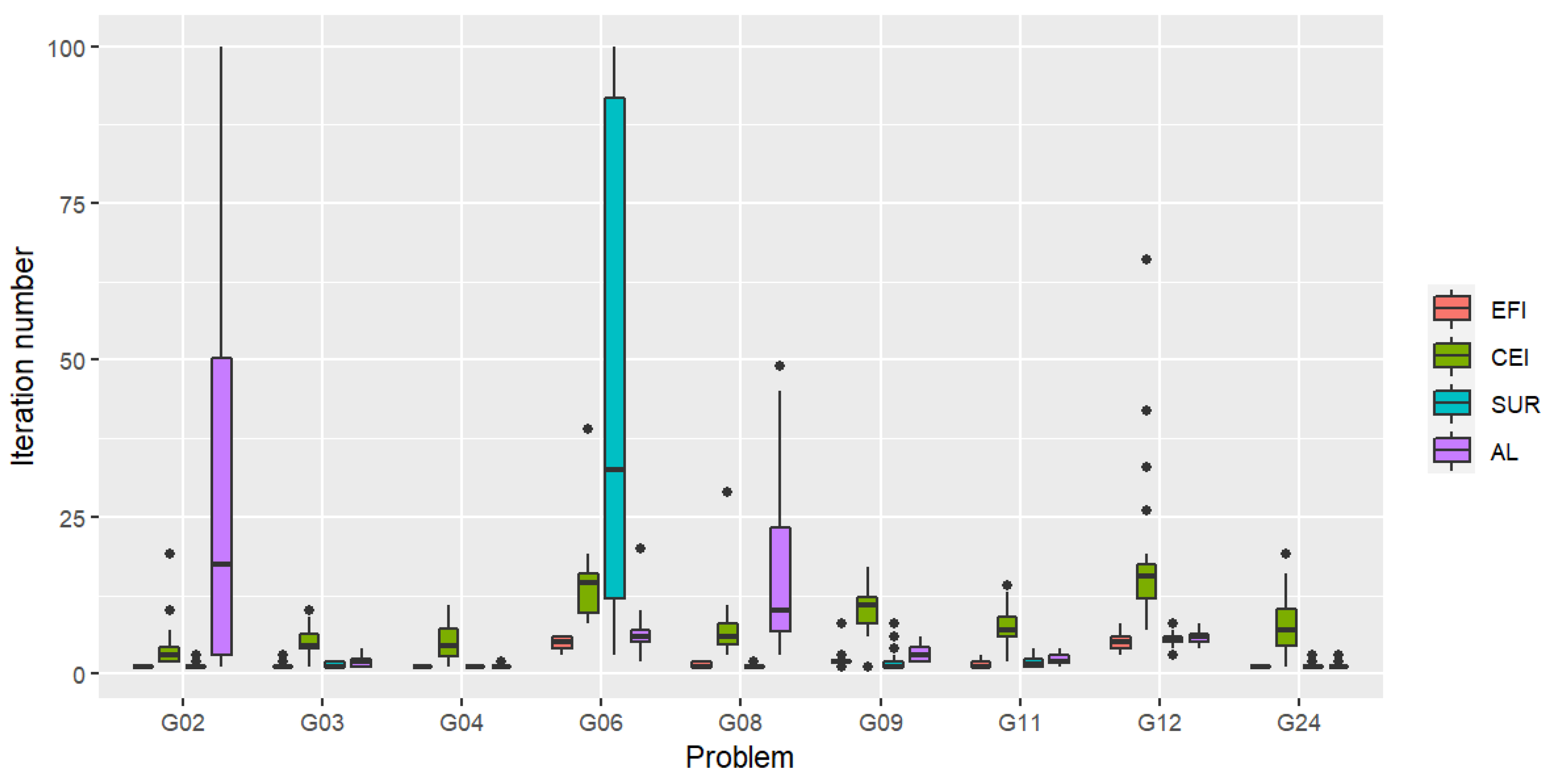
Figure 1 illustrates the distribution of the iteration numbers for which the first feasible solution was found. The value reflects how quickly the process will lead the search to reach feasible regions as the algorithm evolves from outside the feasible regions. From the boxplot, we can see that, overall, EFI could locate a first feasible solution fastest. Except for problems G02 and G06 (when AL and SUR had a problem locating a feasible solution in some trials), CEI found a first feasible solution slowest overall.

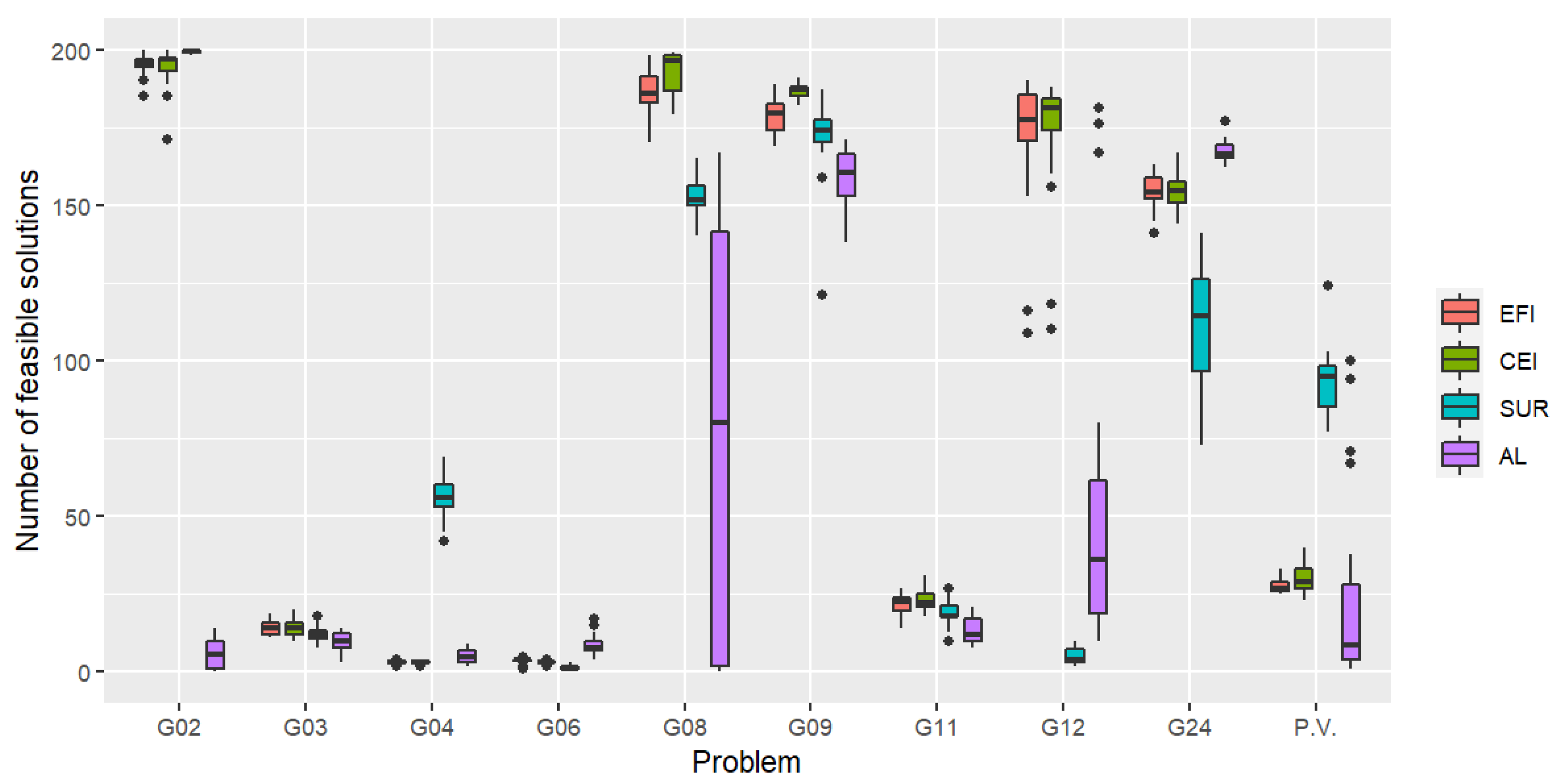
The distribution of the number of feasible solutions out of 100 observations is given in Figure 2.

3.2.2. Scenario 2: Latin Hypercube Initial Design Points

For a more practical and realistic situation, LHSD is used to generate the initial points in the second scenario. In addition to the test problems used in Scenario 1, we also include a practical application of the pressure vessel design optimization problem with four constraints [46]. We shall refer to this problem by the abbreviation P.V. The problem description can be found in Appendix A.2. Results of the best solution found after 200 iterations are given in

Table 5. Results for Scenario 2 after 200 iterations, 20 independent runs. For each problem, the number in brackets in the row “mean” gives the number of trials (out of 20) for which no feasible solutions are found. Mean and standard deviation values represent the best feasible solutions calculated over those trials that can find at least one feasible solution. The row “best” gives the best solution values out of 20 trials.

		EFI	CEI	SUR	AL
G02	mean	−0.364025	−0.364312	−0.359966	−0.015449 (4)
	sd	0.001	$6.4\times {10}^{-4}$	0.003	0.009
	best	−0.364952	−0.364964	−0.363933	−0.026312
G03	mean	−1.004955	−1.004936	−1.002705	−1.004999
	sd	$4.5\times {10}^{-5}$	$6.2\times {10}^{-5}$	0.001	$1.2\times {10}^{-6}$
	best	−1.004995	−1.004993	−1.004749	−1.005
G04	mean	−30,657.612772	−30,656.937017	−30,304.856407	−30,663.376405
	sd	11.773	11.29	110.9	2.117
	best	−30,663.739482	−30,664.743145	−30,509.511844	−30,665.506828
G06	mean	−6918.658417	−6910.902959	−4183.120175	−6961.75848
	sd	24.591	57.828	1492	0.115
	best	−6948.863162	−6952.440967	−6805.861054	−6961.813406
G08	mean	−0.095822	−0.095379	−0.093684	−0.061701 (2)
	sd	$6.9\times {10}^{-6}$	0.002	0.003	0.044
	best	−0.095825	−0.095825	−0.095823	−0.095392
G09	mean	921.327255	865.05661	908.279316	887.020006
	sd	75.58	74	63.3	86.42
	best	771.65775	749.67991	780.921707	762.976464
G11	mean	0.745055	0.74506	0.746072	0.745002
	sd	$3.6\times {10}^{-5}$	$3.3\times {10}^{-5}$	$5.7\times {10}^{-4}$	$1.3\times {10}^{-6}$
	best	0.745022	0.745024	0.745058	0.745
G12	mean	−1	−1	−0.999931	−1
	sd	$2.6\times {10}^{-8}$	$3.1\times {10}^{-8}$	$7.5\times {10}^{-5}$	$4.4\times {10}^{-7}$
	best	−1	−1	−0.999999	−1
G24	mean	−5.506132	−5.506621	−5.455703	−1.942322
	sd	0.001	$8.3\times {10}^{-4}$	0.024	0.620
	best	−5.507517	−5.507572	−5.499659	−3.938104
P.V.	mean	5941.776519	5916.992288	6147.141779	394,221.943568
	sd	63.6	25.6	133	150,000
	best value	5888.547144	5888.510311	5913.191216	300,359.489514

. From the table, we can see that feasible solutions were found by all algorithms in all runs except for problems G02 and G08, where AL failed to locate a feasible solution on 4 and 2 trials, respectively.

In terms of the solution quality, results from a statistical test are reported in

Table 6. Wilcoxon signed-rank test results at the 5% significance level for Scenario 2.

Problem	Results
G02	$EFI\approx CEI\prec SUR$
G03	$AL\prec EFI\approx CEI\prec SUR$
G04	$AL\prec EFI\approx CEI\prec SUR$
G06	$AL\prec EFI\approx CEI\prec SUR$
G08	$EFI\approx CEI\prec SUR$
G09	$AL\approx CEI\prec EFI\approx SUR$
G11	$AL\prec EFI\approx CEI\prec SUR$
G12	$EFI\approx CEI\prec AL\prec SUR$
G24	$EFI\approx CEI\prec SUR\prec AL$
P.V.	$EFI\approx CEI\prec SUR\prec AL$

. We can see that EFI and CEI performed quite similarly except for one case, G09, on which CEI is significantly better than EFI. CEI is best on 6 problems, EFI is best on 5 problems, and AL is best on 5 problems.

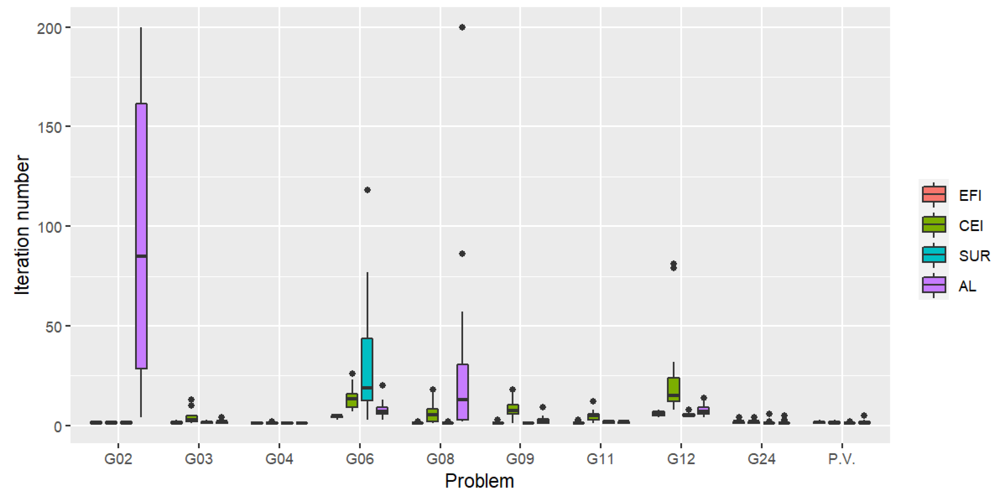
The iteration number for which the first feasible solution is found is shown in Figure 3. It is clear from these boxplots that overall, the fastest algorithm to find the first feasible point is again achieved by EFI. The number of feasible solutions (out of the total number of 200 observations) is given in Figure 4. While AL performed best on 5 problems as mentioned, it did not find a feasible solution on some trials for 2 problems. In addition, AL performed significantly poorly on the pressure vessel problem.

Both EFI and CEI seem to work very well, but CEI tends to search over infeasible regions in the early stages of the algorithm before moving the search towards the feasible region afterwards, while EFI seems to behave in the opposite direction. Finally, although SUR did not fail to find a feasible solution in Scenario 2, none of its solutions is as good as that of other algorithms.

Finally, we summarize the best algorithm for each problem of the two scenarios in

Table 7. Best criteria of each problem due to minimum value achieved.

Problem	Scenario 1	Scenario 2
G02	EFI, CEI	EFI, CEI
G03	AL	AL
G04	AL	AL
G06	AL	AL
G08	EFI, CEI	EFI, CEI
G09	SUR	CEI, AL
G11	AL	AL
G12	EFI, CEI	EFI, CEI
G24	EFI, CEI	EFI, CEI
P.V.	-	EFI, CEI

.

4. Conclusions

In this article, we performed a study on the benchmarking of various CBO algorithms to test the capability of each infill sampling criterion. To that end, experiments with a set of benchmark problems were performed to investigate the impact of the choice of criteria on problems with varying shapes and sizes of feasible regions, ranges of the decision space, as well as initial number of feasible solutions. In light of the results obtained, SUR does not give a satisfactory performance on fast convergence when compared to other methods. AL performed best in several circumstances, but it could not locate a feasible solution on some problem trials. While the performances of EFI and CEI were quite similar, EFI seemed to locate a first feasible solution slightly faster. The obtained results indicate that EFI and CEI could better balance the exploration and exploitation of the objective space and at the same time explore feasible regions more efficiently.

Because of the inherent diversity of these methods, each compared method still has strengths and limitations that leave room for future improvement. Besides the issue of scaling to high-dimensional GPs, another important challenge associated with high-dimensional CBO and/or a large number of constraints is optimization of the infill sampling criterion, which often involves numerical integration methods. To apply CBO to high-dimensional problems, it is therefore necessary to develop methods that scale to high dimensional problems. Consequently, advanced methods on scalable/sparse GPs, local CBO, as well as the strategy used to optimize an infill sampling criterion can be potential research directions [47,48,49,50,51].

In addition, the choice of the initial sampling strategy can also influence the overall quality of the BO [52]. Variance reduction techniques such as those introduced in [53] may also play an important role and affect the performance of algorithms. This can be a potential future direction for benchmarking the CBO algorithm’s performance.

References

- Łukasik, S.; Żak, S. Firefly algorithm for continuous constrained optimization tasks. In International Conference on Computational Collective Intelligence; Springer: Berlin/Heidelberg, Germany, 2009; pp. 97–106. [Google Scholar]
- Tuba, M.; Bacanin, N. Improved seeker optimization algorithm hybridized with firefly algorithm for constrained optimization problems. Neurocomputing 2014, 143, 197–207. [Google Scholar] [CrossRef]
- Askarzadeh, A. A novel metaheuristic method for solving constrained engineering optimization problems: Crow search algorithm. Comput. Struct. 2016, 169, 1–12. [Google Scholar] [CrossRef]
- Arora, S.; Singh, H.; Sharma, M.; Sharma, S.; Anand, P. A new hybrid algorithm based on Grey wolf optimization and crow search algorithm for unconstrained function optimization and feature selection. IEEE Access 2019, 7, 26343–26361. [Google Scholar] [CrossRef]
- Strumberger, I.; Minovic, M.; Tuba, M.; Bacanin, N. Performance of elephant herding optimization and tree growth algorithm adapted for node localization in wireless sensor networks. Sensors 2019, 19, 2515. [Google Scholar] [CrossRef] [PubMed] [Green Version]
- Chung, H.; Shin, K.s. Genetic algorithm-optimized long short-term memory network for stock market prediction. Sustainability 2018, 10, 3765. [Google Scholar] [CrossRef] [Green Version]
- Wang, J.; Cheng, Z.; Ersoy, O.K.; Zhang, P.; Dai, W.; Dong, Z. Improvement analysis and application of real-coded genetic algorithm for solving constrained optimization problems. Math. Probl. Eng. 2018, 2018, 1–16. [Google Scholar] [CrossRef]
- Tuba, E.; Strumberger, I.; Bacanin, N.; Zivkovic, D.; Tuba, M. Brain Storm Optimization Algorithm for Thermal Image Fusion using DCT Coefficients. In Proceedings of the 2019 IEEE Congress on Evolutionary Computation (CEC), Wellington, New Zealand, 10–13 June 2019; pp. 234–241. [Google Scholar]
- Kaur, P.; Sharma, M. Diagnosis of Human Psychological Disorders using Supervised Learning and Nature-Inspired Computing Techniques: A Meta-Analysis. J. Med Syst. 2019, 43, 204. [Google Scholar] [CrossRef]
- Vivekanandan, T.; Iyengar, N.C.S.N. Optimal feature selection using a modified differential evolution algorithm and its effectiveness for prediction of heart disease. Comput. Biol. Med. 2017, 90, 125–136. [Google Scholar] [CrossRef]
- Sharma, M.; Singh, G.; Singh, R. Design and analysis of stochastic DSS query optimizers in a distributed database system. Egypt. Inform. J. 2016, 17, 161–173. [Google Scholar] [CrossRef] [Green Version]
- Močkus, J. On Bayesian methods for seeking the extremum. In Optimization Techniques IFIP Technical Conference; Springer: Berlin/Heidelberg, Germany, 1975; pp. 400–404. [Google Scholar]
- Močkus, J.; Tiesis, V.; Zilinskas, A. The application of Bayesian methods for seeking the extremum. Towards Glob. Optim. 1978, 2, 117–129. [Google Scholar]
- Jones, D.R.; Schonlau, M.; Welch, W.J. Efficient global optimization of expensive black-box functions. J. Glob. Optim. 1998, 13, 455–492. [Google Scholar] [CrossRef]
- Weihs, C.; Herbrandt, S.; Bauer, N.; Friedrichs, K.; Horn, D. Efficient Global Optimization: Motivation, Variations, and Applications. Arch. Data Sci. Ser. 2017, 2, 26. [Google Scholar]
- Bartoli, N.; Kurek, I.; Lafage, R.; Lefebvre, T.; Priem, R.; Bouhlel, M.; Morlier, J.; Stilz, V.; Regis, R. Improvement of efficient global optimization with mixture of experts: Methodology developments and preliminary results in aircraft wing design. In Proceedings of the 17th AIAA/ISSMO Multidisciplinary Analysis and Optimization Conference, Washington, DC, USA, 13–17 June 2016. [Google Scholar]
- Quttineh, N.H.; Holmström, K. Implementation of a One-Stage Efficient Global Optimization (EGO) Algorithm; Technical Report 2; Linköping University: Linkoping, Sweden, 2009. [Google Scholar]
- Hebbal, A.; Brevault, L.; Balesdent, M.; Taibi, E.G.; Melab, N. Efficient Global Optimization Using Deep Gaussian Processes. In Proceedings of the 2018 IEEE Congress on Evolutionary Computation (CEC), Rio de Janeiro, Brazil, 8–13 July 2018; pp. 1–8. [Google Scholar]
- Mehdad, E.; Kleijnen, J. Efficient Global Optimization for Black-Box Simulation Via Sequential Intrinsic Kriging. SSRN Electron. J. 2015, 69, 1725–1737. [Google Scholar] [CrossRef] [Green Version]
- Ur Rehman, S.; Langelaar, M. Efficient global robust optimization of unconstrained problems affected by parametric uncertainties. Struct. Multidiscip. Optim. 2015, 52, 319–336. [Google Scholar] [CrossRef] [Green Version]
- Jeong, S.; Obayashi, S. Efficient global optimization (EGO) for multi-objective problem and data mining. In Proceedings of the 2005 IEEE Congress on Evolutionary Computation, Scotland, UK, 2–5 September 2005; Volume 3, pp. 2138–2145. [Google Scholar]
- ur Rehman, S.; Langelaar, M. Expected improvement based infill sampling for global robust optimization of constrained problems. Optim. Eng. 2017, 18, 723–753. [Google Scholar] [CrossRef] [Green Version]
- Ye, Q.; Pan, H.; Liu, C. A framework for final drive simultaneous failure diagnosis based on fuzzy entropy and sparse bayesian extreme learning machine. Comput. Intell. Neurosci. 2015, 2015, 427965. [Google Scholar] [CrossRef] [Green Version]
- Kopsiaftis, G.; Protopapadakis, E.; Voulodimos, A.; Doulamis, N.; Mantoglou, A. Gaussian process regression tuned by bayesian optimization for seawater intrusion prediction. Comput. Intell. Neurosci. 2019, 2019, 2859429. [Google Scholar] [CrossRef]
- Chen, Z. An overview of bayesian methods for neural spike train analysis. Comput. Intell. Neurosci. 2013, 2013. [Google Scholar] [CrossRef] [Green Version]
- Schonlau, M.; Welch, W.J.; Jones, D.R. Global versus local search in constrained optimization of computer models. Lect. Notes Monogr. Ser. 1998, 34, 11–25. [Google Scholar]
- Gardner, J.R.; Kusner, M.J.; Xu, Z.; Weinberger, K.Q.; Cunningham, J.P. Bayesian Optimization with Inequality Constraints. In Proceedings of the 31st International Conference on International Conference on Machine Learning, Beijing, China, 21–26 June 2014. [Google Scholar]
- Sasena, M.J.; Papalambros, P.; Goovaerts, P. Exploration of metamodeling sampling criteria for constrained global optimization. Eng. Optim. 2002, 34, 263–278. [Google Scholar] [CrossRef]
- Priem, R.; Bartoli, N.; Diouane, Y. On the Use of Upper Trust Bounds in Constrained Bayesian Optimization Infill Criteria. In Proceedings of the AIAA Aviation 2019 Forum, Dallas, TX, USA, 17–21 June 2019; p. 2986. [Google Scholar]
- Srinivas, N.; Krause, A.; Kakade, S.; Seeger, M. Gaussian Process Optimization in the Bandit Setting: No Regret and Experimental Design. In Proceedings of the 27th International Conference on International Conference on Machine Learning, Haifa, Israel, 21–24 June 2010; pp. 1015–1022. [Google Scholar]
- Gramacy, R.; Lee, H. Optimization Under Unknown Constraints. Bayesian Stat. 2011, 9, 229–256. [Google Scholar]
- Gelbart, M.A.; Snoek, J.; Adams, R.P. Bayesian Optimization with Unknown Constraints. In Proceedings of the Thirtieth Conference on Uncertainty in Artificial Intelligence, Quebec City, QC, Canada, 23–27 July 2014; pp. 250–259. [Google Scholar]
- Hernández-Lobato, J.M.; Gelbart, M.A.; Hoffman, M.W.; Adams, R.P.; Ghahramani, Z. Predictive entropy search for bayesian optimization with unknown constraints. In Proceedings of the 32nd International Conference on Machine Learning (ICML), Lille, France, 6–11 July 2015; pp. 1699–1707. [Google Scholar]
- Hernández-Lobato, J.M.; Hoffman, M.W.; Ghahramani, Z. Predictive entropy search for efficient global optimization of black-box functions. In Proceedings of the Advances in Neural Information Processing Systems, Montreal, QC, Canada, 8–13 December 2014; pp. 918–926. [Google Scholar]
- Lam, R.; Willcox, K. Lookahead bayesian optimization with inequality constraints. In Proceedings of the Advances in Neural Information Processing Systems, Long Beach, CA, USA, 4–9 December 2017; pp. 1890–1900. [Google Scholar]
- Ariafar, S.; Coll-Font, J.; Brooks, D.; Dy, J. An ADMM Framework for Constrained Bayesian Optimization. In Proceedings of the NIPS Workshop on Bayesian Optimization, Long Beach, CA, USA, 9 December 2017. [Google Scholar]
- Jiao, R.; Zeng, S.; Li, C.; Jiang, Y.; Jin, Y. A complete expected improvement criterion for Gaussian process assisted highly constrained expensive optimization. Inf. Sci. 2019, 471, 80–96. [Google Scholar] [CrossRef]
- Picheny, V. Multiobjective optimization using Gaussian process emulators via stepwise uncertainty reduction. Stat. Comput. 2013, 25, 1265–1280. [Google Scholar] [CrossRef] [Green Version]
- Picheny, V. A Stepwise uncertainty reduction approach to constrained global optimization. In Proceedings of the Seventeenth International Conference on Artificial Intelligence and Statistics, Reykjavik, Iceland, 22–25 April 2014; Volume 33, pp. 787–795. [Google Scholar]
- Gramacy, R.B.; Gray, G.A.; Digabel, S.L.; Lee, H.K.H.; Ranjan, P.; Wells, G.; Wild, S.M. Modeling an Augmented Lagrangian for Blackbox Constrained Optimization. Technometrics 2016, 58, 1–11. [Google Scholar] [CrossRef]
- Picheny, V.; Ginsbourger, D.; Krityakierne, T. Comment: Some Enhancements Over the Augmented Lagrangian Approach. Technometrics 2016, 58, 17–21. [Google Scholar] [CrossRef]
- Rasmussen, C.; Williams, C. Gaussian Processes for Machine Learning; MIT Press: Cambridge, MA, USA, 2006; p. 248. [Google Scholar]
- Roustant, O.; Ginsbourger, D.; Deville, Y. DiceKriging, DiceOptim: Two R Packages for the Analysis of Computer Experiments by Kriging-Based Metamodeling and Optimization. J. Stat. Softw. 2013, 51, 1–55. [Google Scholar] [CrossRef] [Green Version]
- Gelbart, M.A. Constrained Bayesian Optimization and Applications. Ph.D. Thesis, Harvard University, Cambridge, MA, USA, 2015. [Google Scholar]
- Damblin, G.; Couplet, M.; Iooss, B. Numerical studies of space filling designs: Optimization of Latin Hypercube Samples and subprojection properties. J. Simul. 2013, 7, 276–289. [Google Scholar] [CrossRef] [Green Version]
- Ke, X.; Zhang, Y.; Li, Y.; Du, T. Solving design of pressure vessel engineering problem using a fruit fly optimization algorithm. Int. J. Simul. Syst. Sci. Technol. 2016, 17, 5. [Google Scholar] [CrossRef]
- Quiñonero-Candela, J.; Rasmussen, C.E. A unifying view of sparse approximate Gaussian process regression. J. Mach. Learn. Res. 2005, 6, 1939–1959. [Google Scholar]
- Wang, K.; Pleiss, G.; Gardner, J.; Tyree, S.; Weinberger, K.Q.; Wilson, A.G. Exact Gaussian processes on a million data points. In Proceedings of the Advances in Neural Information Processing Systems, Vancouver, BC, Canada, 8–14 December 2019; pp. 14622–14632. [Google Scholar]
- Krityakierne, T.; Ginsbourger, D. Global optimization with sparse and local Gaussian process models. In International Workshop on Machine Learning, Optimization and Big Data; Springer: Cham, Switzerland, 2015; pp. 185–196. [Google Scholar]
- Eriksson, D.; Pearce, M.; Gardner, J.; Turner, R.D.; Poloczek, M. Scalable global optimization via local bayesian optimization. In Proceedings of the Advances in Neural Information Processing Systems, Vancouver, BC, Canada, 8–14 December 2019; pp. 5496–5507. [Google Scholar]
- Krityakierne, T.; Baowan, D. Aggregated GP-based Optimization for Contaminant Source Localization. Oper. Res. Perspect. 2020, 7, 100151. [Google Scholar] [CrossRef]
- Bossek, J.; Doerr, C.; Kerschke, P. Initial Design Strategies and their Effects on Sequential Model-Based Optimization. arXiv 2020, arXiv:2003.13826. [Google Scholar]
- Shields, M.D.; Zhang, J. The generalization of Latin hypercube sampling. Reliab. Eng. Syst. Saf. 2016, 148, 96–108. [Google Scholar] [CrossRef] [Green Version]
Figure 1.
Distribution of the iteration number for which the first feasible solution is found (Scenario 1) for the criteria: expected feasible improvement (EFI), constrained expected improvement (CEI), stepwise uncertainty reduction (SUR), and augmented Lagrangian (AL). The lower the plot, the faster the criterion is in finding the first feasible solution.
Figure 2.
Distribution of the number of feasible solutions over the course of 100 iterations (Scenario 1). The higher the plot, the more frequently the feasible solutions are visited.
Figure 3.
Distribution of the iteration number for which the first feasible solution is found (Scenario 2). The lower the plot, the faster the criterion is in finding the first feasible solution.
Figure 4.
Distribution of the number of feasible solutions over the course of 200 iterations (Scenario 2). The higher the plot, the more frequently the feasible solutions are visited.