On Confinement and Quarantine Concerns on an SEIAR Epidemic Model with Simulated Parameterizations for the COVID-19 Pandemic

Abstract

This paper firstly studies an SIR (susceptible-infectious-recovered) epidemic model without demography and with no disease mortality under both total and under partial quarantine of the susceptible subpopulation or of both the susceptible and the infectious ones in order to satisfy the hospital availability requirements on bed disposal and other necessary treatment means for the seriously infectious subpopulations. The seriously infectious individuals are assumed to be a part of the total infectious being described by a time-varying proportional function. A time-varying upper-bound of those seriously infected individuals has to be satisfied as objective by either a total confinement or partial quarantine intervention of the susceptible subpopulation. Afterwards, a new extended SEIR (susceptible-exposed-infectious-recovered) epidemic model, which is referred to as an SEIAR (susceptible-exposed-symptomatic infectious-asymptomatic infectious-recovered) epidemic model with demography and disease mortality is given and focused on so as to extend the above developed ideas on the SIR model. A proportionally gain in the model parameterization is assumed to distribute the transition from the exposed to the infectious into the two infectious individuals (namely, symptomatic and asymptomatic individuals). Such a model is evaluated under total or partial quarantines of all or of some of the subpopulations which have the effect of decreasing the number of contagions. Simulated numerical examples are also discussed related to model parameterizations of usefulness related to the current COVID-19 pandemic outbreaks.

1. Introduction

Epidemic mathematical models in different formal frameworks are of crucial interest in recent decades [1,2]. Such mentioned formal frameworks include, for instance, differential, difference and differential/difference hybrid equations, dynamic systems, control theory [3,4,5,6,7,8,9,10,11,12,13,14,15,16,17,18,19,20], computation [7], and information theory [21,22,23,24,25,26,27,28] as well as combined mathematical analysis of epidemic spreading and control design tools [21,22,27,28,29,30,31,32,33,34,35,36]. One of the objectives of such models is to investigate and predict the evolution of epidemic infectious diseases in humans, animals, or plants as well as to elucidate how the interventions, like quarantine actions or regular and impulsive vaccination and treatment controls, can avoid or mitigate their contagious propagation (See References [1,2,11,13,15,17,18,19,20,25,26,27,28,29,30,31,32,33,34,35,36]). It can be pointed out that the quarantine and the confinement interventions are qualitatively similar to using impulsive vaccination and treatment controls since all or a part of a targeted subpopulation (typically, the susceptible one or the infectious one or fractions of them) is removed from its associate compartment and the viewable effect is a re-initialization of the corresponding trajectory solution under fewer contagious contacts. Another beneficial effect is that the transmission rate decreases to lower levels because of the mentioned decrease in the number of contacts. The previously mentioned control intervention are very relevant concerning the disease temporary evolution and its steady-state reachable numbers of the various subpopulations since they can increase the values of the transmission rate being compatible with a basic reproduction number being less than unity. This property implies that the disease-free equilibrium point is a global attractor and the disease becomes asymptotically removed as a result. Those above issues have been important in the last months with regard to the evolution of the COVID-19 pandemic around the world (See References [27,29,37,38,39,40,41,42,43,44,45,46,47,48,49,50,51]). In particular, an “ad hoc” SEIR model parameterization related to the COVID-19 pandemic is investigated in Reference [37] including delayed re-susceptibility caused by the infection. Additionally, a kind of autoregressive model average model (ARMA), known as an ARIMA model for prediction of COVID-19, is presented and simulated in Reference [38] for the data of several countries. The effects of different phases of quarantine actions in the values of the transmission rate are studied in Reference [39]. See Reference [42] for a discussion of related simulated numerical results on the COVID-19 outbreak in Italy. Some results have been recently reported on reaction-diffusion epidemic models of usefulness fore dengue [52], on delayed diffusive epidemic models [53], and on multi-group epidemic discrete models with time delays [54]. (See also related references therein).

It can be pointed out that there are links in the descriptions of epidemic models to symmetry and asymmetry concepts with different interpretations. For instance, in Reference [13], the problem of patchy epidemic environments in the multi-node case where there are in-flux and out-flux of populations between different nodes (for instance, with each node describing distinct towns or regions) is focused on. The most general assumption involved is that the matrices of population travelling interchange are asymmetric in the most general case, but they can be symmetric in particular. In Reference [55], a close problem is focused on for epidemic models describing a network with more than one node and the concepts of symmetry and asymmetry play a role in the mathematical description of the proposed model. On the other hand, in Reference [56], the case of reported versus unreported infective cases is calculated. In the case of time-invariant model parameterizations, such a ratio becomes invariant for both the time-instantaneous tests and the time- accumulated tests interpreted as a certain symmetry property. Generally speaking, symmetry is equivalent to an invariance of a certain quantity under transformations. In that way, a related property associated with a number of common epidemic models is their invariance under certain transformations of variables, which is a property that applies even for models of a single node. Assume, for instance, a true-mass action epidemic model [43] with a typical bilinear incidence of the form $\beta SI/N$ where $\beta$ is the transmission rate and S and I are the susceptible and infectious instantaneous numbers and $N$ is the total population assumed constant through time. Furthermore, assume that the above model is changed to a normalized one for all the subpopulations leading to the transformed variables $s=S/N$, $i=I/N$ etc. It can be easily seen that the form of the equations remains invariant with the redefined transmission rate ${\beta }_n=\beta N$. Such an idea is applicable even to epidemic models of a single node.

The related existing bibliography on epidemic modelling is abundant and very rich including a variety of epidemic models with several coupled subpopulations including the susceptible, the infectious, and the recovered ones as an elementary starting basis in the simpler SIR epidemic models. Further generalizations lead to the so-called SEIR models, which include the exposed subpopulation (those who do not have external symptoms yet) as a new subpopulation. More complex models, such as SEIADR-type models, which include the asymptomatic infectious and the infective dead subpopulations, have been designed and discussed, for instance, for Ebola disease [15,16]. On the other hand, Covid-19 is an infectious disease caused by a newly discovered coronavirus at the end of 2019. The first outbreak was reported in Wuhan (China) and then it extended worldwide very fast [57]. At this time, there is no vaccine nor effective treatment available while social distancing, isolation, and quarantine have been revealed to be the most important measurements to counteract its spread. Despite the current death rate of the disease being around 3–4%, acute symptoms may lead to intensive care unities (ICU’s) admission to many seriously infected patients, which provokes the overflow of these units and a situation of stress in the health system of many countries where the situation of their health systems is becoming really difficult over recent months because of the lack of beds, material, and staff for the abundant, seriously infected people.

The main objective of this paper is to propose and to investigate a new SEIAR epidemic model with demography, which is a generalized SEIR (susceptible-exposed-infectious-recovered). Such a model includes asymptomatic infectious (A) and eventual illness mortality. All the formulations are developed in a deterministic framework of differential equations with finite jumps in their solutions. A fraction of the exposed subpopulation has a transition to the symptomatic infectious subpopulation while its complementary to unity fraction has a transition to the asymptomatic one. The main results concern the study of the model under, in general, partial quarantines. Total quarantine actions and confinement interventions are considered as particular cases being governed, in each particular situation, by the choices of the gains, which describe the decrease of subpopulation levels subject to eventual reception or transmission of new contagions. Such gains are designed in such a way that the foreseen fraction of the infectious needing hospital care are upper-bounded by a function, which describes the hospital availability on beds and other means, like staff, available amounts and qualification, number of respirators, etc. Before the presentation and discussion of the new proposed SEIAR model, two simple illustrative examples on partial or total quarantines are given on a simpler SIR model without demography and with no mortality.

The paper is organized as follows. Section 2 states and briefly describes the simple mentioned SIR model under total or partial quarantine of the susceptible and infectious in order to satisfy the objective that a weighted proportion of the infectious subpopulation is less than a certain upper-bound defined by hospital treatment considerations. Section 3 presents the proposed SEIAR model, which includes the exposed and the asymptomatic subpopulations subject to demography and eventual mortality so that it generalizes the previously discussed SIR model. The properties of positivity and boundedness of the state trajectory solution are stated and proved. Section 4 studies the model under partial or total quarantines of some or all the subpopulations so that a hospital management objective on temporary availability of technical means and bed disposal can be fulfilled. Section 5 presents and discusses some numerically worked examples under model parameterizations of the COVID-19 pandemic to test the efficiency of several quarantine interventions. Lastly, conclusions end the paper. Appendix A and Appendix B with details of some auxiliary calculations are also given.

2. A Quarantined SIR Epidemic Model

The effects of total or partial quarantine interventions imply that the transmission rates decrease since the number of contagious contacts decreases. See, for instance, References [38,39]. The quarantines on the susceptible have the qualitative effect of an impulsive vaccination since part of the susceptible population is kept away of infective contacts. This is equivalent to reduce, in practice, along a short time interval (instantaneously in an ideal impulsive model), the susceptible subpopulation. Similarly, quarantines on the infectious are similar to impulsive treatment actions on the infectious subpopulation, which is equivalent to reduce its numbers in short time intervals or instantaneously in the ideal case (See References [11,15,18,19]). Quarantine of infectious agents is also referred to as their isolation. However, in order to unify the nomenclature along the paper, the term quarantine will be used for all populations.

Example 1 below on an SIR model without mortality is given as an introductory one to fix some basic ideas about quarantine decisions. Such decisions might be made on both susceptible and infectious decisions based on the hospital management regarding availability of beds and other hospital technical means necessary for infection treatment on seriously infected individuals. The solution for this model is obtained directly from the differential equations and it is then extended to more general SEIR models including quarantine actions and demography with the presence of exposed and asymptomatic individuals. It can be pointed out that the solution for an SIR model with demography has been obtained in Reference [5] by its reduction to an Abel-type equation by using a power-series perturbation approach.

2.1. Example 1 (An SIR Epidemic Model without Demography Subject to Monitored Quarantine)

Consider the subsequent SIR (Susceptible “S”- Infectious “I”- Recovered “R”) without demography and disease mortality:

$$\begin{gathered} \dot{S}\left(t\right)=-\beta S\left(t\right)I\left(t\right) \\ \dot{I}\left(t\right)=\beta S\left(t\right)I\left(t\right)-\mathsf{\gamma }I\left(t\right) \\ \dot{R}\left(t\right)=\mathsf{\gamma }I\left(t\right) \end{gathered}$$

(1)

with $S\left(0\right)=S_0$, $I\left(0\right)=I_0\ge 0$ and $R\left(0\right)=R_0\ge 0$ with $\mathit{min}\left(S_0,I_0,R_0\right)\ge 0$, where $\beta$ and $\mathsf{\gamma }$ are the transmission rate and the recovery rate, respectively. The total population is $N\left(t\right)=S\left(t\right)+I\left(t\right)+R\left(t\right)$; $\forall t\in R_{0+}$ with $N\left(t\right)=N\left(0\right)=N_0$ being constant $\forall t\in R_{0+}$ in view of (1). The solution of (1) is:

$$\begin{gathered} S\left(t\right)=e^{-\beta {\displaystyle {\int }_0^{t}I\left(\tau \right) d\tau }}{S}_0 \\ I\left(t\right)=e^{\beta {\displaystyle {\int }_0^{t}S\left(\tau \right) d\tau -\mathsf{\gamma }t}}{I}_0=e^{-\mathsf{\gamma }t}{e}^{\beta S_0{\displaystyle {\int }_0^t{e}^{-\beta {\displaystyle {\int }_0^{\tau }I\left(\sigma \right) d\sigma }} d\tau }}{I}_0 \\ R\left(t\right)=e^{\mathsf{\gamma }{\displaystyle {\int }_0^{t}I\left(\tau \right)d\tau }}{R}_0. \end{gathered}$$

(2)

Let $I_h\left(t\right)=\rho \left(t\right)I\left(t\right)$ the estimated fraction of infectious which require hospital care at time $t$ (referred to as the “seriously ill infectious subpopulation”) and ${\overline{I}}_h\left(t\right)$ the upper-bound of hospital admission availability at time $t$. Note the following simple result which is concerned with an eventual quarantine intervention of all the susceptible individuals:

Proposition 1. 

Assume that, for a given $\rho \left(t\right)\in \left(0 ,1\right]$ and an availability upper-bound ${\overline{I}}_h\left(t\right)$, it is possible to hospitalize all the seriously ill infectious subpopulations at time t via susceptible quarantine of all the susceptible subpopulations at time $t_0=0$, if $I_0\le \frac{e^{\mathsf{\gamma }t}}{\rho \left(t\right)}{\overline{I}}_h\left(t\right)$ $;\forall t\in R_{0+}$.

Proof. 

Assume that $S_0=0$, that is, a total quarantine of the existing susceptible subpopulation at time $t_0=0$, or absence of an initial susceptibility for an eventual contagion. Then $\rho \left(t\right)I\left(t\right)=\rho \left(t\right)e^{-\mathsf{\gamma }t}{I}_0\le {\overline{I}}_h\left(t\right)$ from Equation (2) for any given $t\in R_{0+}$ if $I_0\le \frac{e^{\mathsf{\gamma }t}}{\rho \left(t\right)}{\overline{I}}_h\left(t\right)$ with initial immune amounts given by $R_0=N_0-I_0\ge \underset{t\in R_{0+}}{\mathit{max}}\left(0,N_0-\frac{e^{\mathsf{\gamma }t}}{\rho \left(t\right)}{\overline{I}}_h\left(t\right)\right)$. □

In general, it might not be necessarily a total quarantine on the susceptible to accomplish with the hospital management requirements provided that the number of initial infections is small enough according to Proposition 1. In this sense, Proposition 1 might be easily generalized to the case of partial quarantine of the susceptible. It can be necessary to keep the hospital bed availability at time $t$ along a time interval of a length of at least ${\mathsf{\gamma }}^{-1}$, which is the recovery average period or up until some time exceeding $t$ along the lasting of the most serious period of the illness force. The subsequent Proposition 2 is based on a partial withdrawal of the initial susceptible amounts from the contagion scenario via a quantifying parameter $\mathsf{\lambda }\in \left[0,1\right]$ of the fraction population to withdraw from the contagion environment at the time instant where a quarantine intervention is decided. For instance, if a quarantine is decided on the susceptible subpopulation at time $t_1$, then $S\left(t_1^{+}\right)=\left(1-\mathsf{\lambda }\right)S\left(t_1^{-}\right)$, where $S\left(t_1^{+}\right)=\underset{t\to t_1^{+}}{\mathit{lim}}S\left(t\right)$ and $S\left(t_1^{-}\right)=S\left(t_1\right)=\underset{t\to t_1^{-}}{\mathit{lim}}S\left(t\right)$ and the instantaneous net change of the susceptible subpopulation at $t_1$ is $\Delta S\left(t_1\right)=S\left(t_1^{+}\right)-S\left(t_1^{-}\right)=-\mathsf{\lambda }S\left(t_1^{-}\right)$. In the following, we show an alternative and confluent interpretation to the finite jumps in the solution decreases the susceptible candidate individuals available for contagion at the time instant $t=t_1$. A Dirac impulse of amplitude $-\mathsf{\lambda }S\left(t_1^{-}\right)$, namely $-\mathsf{\lambda }\delta \left(t-t_1\right)S\left(t_1^{-}\right)$, with $\delta \left(.\right)$ denoting the Dirac delta distribution is applied to the time–derivative of $S\left(t\right)$ at $t=t_1$, which is physically equivalent to the injection of such an instantaneous impulsive vaccination on the susceptibility [43]. Proposition 2 is concerned with a quarantine intervention at $t=0$ on the susceptible subpopulation, which leads to the eventual existence bounded discontinuity of the solution at $t=0$ and an impulsive corresponding time-derivative as a result. The piecewise continuous solution of the differential system is still unique since the finite jump at the discontinuity is calculated explicitly with its left and right limits at the discontinuity point.

Proposition 2. 

Assume that $S\left(0^{-}\right)=S_0^{-}=S_0$ and $S\left(0^{+}\right)=S_0^{+}=\left(1-\mathsf{\lambda }\right)S_0$ for some $\mathsf{\lambda }\in \left[0 , 1\right]$, where $\mathsf{\lambda }{S}_0$ is the amount of initial susceptible submitted to quarantine at the initial time instant $t_0=0$. Then, the following properties hold.

(i) 

The constraint$\rho \left(t\right)I\left(t\right)\le {\overline{I}}_h\left(t\right)$is fulfilled for some given$t\in R_{+}$if$\mathsf{\lambda }\ge {\mathsf{\lambda }}_m=\mathit{max}\left(1-\frac{\mathit{ln} {\overline{I}}_h\left(t\right)-\mathit{ln}\rho \left(t\right)+\mathsf{\gamma }t}{\beta S_0{\displaystyle {\int }_0^t{e}^{-\beta {\displaystyle {\int }_0^{\tau }I\left(\sigma \right) d\sigma }} d\tau }} , 0\right)$provided that$I_0\le \frac{e^{\mathsf{\gamma }t}}{\rho \left(t\right)}{\overline{I}}_h\left(t\right)$.

(ii) 

The constraint$\rho \left(\theta \right)I\left(\theta \right)\le {\overline{I}}_h\left(\theta \right)$is fulfilled for$\theta \in {\left[t,t+{\mathsf{\gamma }}^{-1}+\eta \right]}^{}$for any given$\eta \in {\left[{\eta }_0-{\mathsf{\gamma }}^{-1} , {\eta }_1\right]}^{}$and some prefixed${\eta }_0, {\eta }_1\in R_{0+}$if and only if$\mathsf{\lambda }\ge {\mathsf{\lambda }}_{m\theta }=\mathit{max}\left(1-\underset{t\le \xi \le t+{\mathsf{\gamma }}^{-1}+\eta }{\mathit{inf}}\frac{\mathit{ln} {\overline{I}}_h\left(\xi \right)-\mathit{ln}\rho \left(\xi \right)+\mathsf{\gamma }\xi -\mathit{ln}{I}_0}{\beta S_0{\displaystyle {\int }_0^{\xi }{e}^{-\beta {\displaystyle {\int }_0^{\tau }I\left(\sigma \right) d\sigma }} d\tau }} , 0\right)$. If$\rho \left(\theta \right)=\rho \left(t\right)$and${\overline{I}}_h\left(\theta \right)={\overline{I}}_h\left(t\right)$; $\forall \theta \in {\left[t,t+{\mathsf{\gamma }}^{-1}+\eta \right]}^{}$then the constraint$\rho \left(\theta \right)I\left(\theta \right)\le {\overline{I}}_h\left(\theta \right)$is fulfilled for$\theta \in {\left[t,t+{\mathsf{\gamma }}^{-1}+\eta \right]}^{}$if$\mathsf{\lambda }\ge \mathit{max}\left(1-\frac{\mathit{ln} {\overline{I}}_h\left(t\right)-\mathit{ln}\rho \left(t\right)+\mathsf{\gamma }t-\mathit{ln}{I}_0}{\beta S_0{\displaystyle {\int }_0^{t+{\mathsf{\gamma }}^{-1}+\eta }{e}^{-\beta {\displaystyle {\int }_0^{\tau }I\left(\sigma \right) d\sigma }} d\tau }} , 0\right)$.

Proof. 

The hospital management availability objective is fulfilled at time t if and only if:

$$\rho \left(t\right)e^{-\mathsf{\gamma }t}{e}^{\beta \left(1-\mathsf{\lambda }\right)S_0{\displaystyle {\int }_0^t{e}^{-\beta {\displaystyle {\int }_0^{\tau }I\left(\sigma \right) d\sigma }} d\tau }}{I}_0\le {\overline{I}}_h\left(t\right)$$

(3)

or, equivalently, if and only if

$$\mathit{ln}\rho \left(t\right)-\mathsf{\gamma }t+\beta \left(1-\mathsf{\lambda }\right)S_0{\displaystyle {\int }_0^t{e}^{-\beta {\displaystyle {\int }_0^{\tau }I\left(\sigma \right) d\sigma }} d\tau }+\mathit{ln}{I}_0\le \mathit{ln} {\overline{I}}_h\left(t\right)$$

(4)

which is satisfied for some $\mathsf{\lambda }\in \left[0 , 1\right]$ if and only if $\mathsf{\lambda }\ge {\mathsf{\lambda }}_m$. Property (i) has been proved. Property (ii) is a direct extension of Property (ii). □

Related to Proposition 2, note that $S_0^{+}/S_0^{-}=1-\mathsf{\lambda }$ and $\Delta S_0/S_0^{-}=\left(S_0^{+}-S_0^{-}\right)/S_0^{-}=-\mathsf{\lambda }$. Then, $1-\mathsf{\lambda }$ is the instantaneous relative variation of the susceptible subpopulation at the impulsive time instant $t_0=0$ where a quarantine intervention is applied on the susceptible. In the same way, $-\mathsf{\lambda }$ is the relative negative decrement of the population at $t_0=0$ because of the quarantine action. Similar interpretations apply for any quarantined subpopulation as it will be discussed later on in this section and in the remaining sections.

Note that Proposition 1 describes the total initial quarantine of the susceptible as a particular case in Proposition 2 with $\mathsf{\lambda }=1$. Proposition 2 establishes a guaranteed fraction of the susceptible submitted to quarantine for achieving the hospital availability of serious cases at a certain time instant or time interval.

Example 1 is now extended with two combined quarantine interventions on the susceptible and infectious subpopulations, respectively. For exposition simplicity, it is assumed in example 1 and in example 2 below that the transmission rate becomes constant. In practice, such a parameter decreases as the number of infectious-susceptible contacts decreases and increases since such a number increases. This fact would be taken into account along Section 4 and Section 5 where a more general epidemic model will be discussed.

2.2. Example 2 (A Partial Quarantine on the Susceptible Followed by a Later Partial Quarantine on the Infectious)

Example 1 can be generalized by programming a first partial quarantine on the susceptible and a later partial quarantine on the infectious so that certain susceptible amounts can be protected from the infection and some infectious are then taken apart from the successive propagation of the infection. This makes sense if there are relatively few susceptible and relevant infectious numbers in the time where the action starts and it is the considered case. Later on, it is considered the case when there are initially relatively few infectious cases, which is a fraction of known cases submitted to quarantine, while, later on, as the infection progresses, there are relevant numbers of susceptible cases, which need to be protected as the infectious cases are increasing. This has been recently the case in many countries around the world concerning the COVID19 has out-broken from epidemic to pandemic [38,46,47,48,49,50].

Thus, assume that, at a time instant $t_1$, a fraction $\mathsf{\lambda }\left(t_1\right)S\left(t_1\right)$ is submitted to quarantine on the interval $\left[t_1,t_3\right]$ and that, at a time instant $t_2\in \left[t_1 ,t_3\right)$, a fraction $\rho \left(t_2\right)I\left(t_2\right)$ of the infectious cases is submitted to quarantine on the time interval $\left[t_2,t_3\right]$. Assume, with no loss in generality, that the initial conditions are taken at $t_0=0$. The question arises is how to choose reasonably $\mathsf{\lambda }\left(t_1\right)\in \left(0 , 1\right)$, $\delta \left(t_2\right)\in \left(0, 1\right)$, T₀ = t₁ – t₀, and $T_1=t_2-t_1$ such that $\rho \left(t\right)I\left(t\right)\le {\overline{I}}_h\left(t\right)$, $\forall t\in {\left[t_3,t_3+{\mathsf{\gamma }}^{-1}+\eta \right]}^{}$ for any $\eta \in {\left[{\eta }_0-{\mathsf{\gamma }}^{-1} , {\eta }_1\right]}^{}$ and some prefixed ${\eta }_0, {\eta }_1\in R_{0+}$. The solution trajectory obeys from (1) the following set of equations of which there is at least one per subpopulation, which depends on the infectious evolution only from the initial conditions, in view of Equation (2).

$$S\left(t\right)=e^{-\beta {\displaystyle {\int }_0^{t}I\left(\tau \right) d\tau }}{S}_0;\forall t\in \left[0,t_1\right)$$

(5)

$$S\left(t_1^{+}\right)=\left(1-\mathsf{\lambda }\left(t_1\right)\right)S\left(t_1^{-}\right)=\left(1-\mathsf{\lambda }\left(t_1\right)\right)e^{-\beta {\displaystyle {\int }_0^{t_1}I\left(\tau \right) d\tau }}{S}_0$$

(6)

$$S\left(t\right)=e^{-\beta {\displaystyle {\int }_{t_1}^{t}I\left(\tau \right) d\tau }}S\left(t_1^{+}\right)=e^{-\beta {\displaystyle {\int }_{t_1}^{t}I\left(\tau \right) d\tau }}\left(1-\mathsf{\lambda }\left(t_1\right)\right)S\left(t_1^{-}\right)=e^{-\beta {\displaystyle {\int }_0^{t}I\left(\tau \right) d\tau }}\left(1-\mathsf{\lambda }\left(t_1\right)\right)S_0;\forall t\in \left[t_1,\infty \right)$$

(7)

$$I\left(t\right)=e^{\beta {\displaystyle {\int }_0^{t}S\left(\tau \right) d\tau -\mathsf{\gamma }t}}{I}_0=e^{-\mathsf{\gamma }t}{e}^{\beta S_0{\displaystyle {\int }_0^t{e}^{-\beta {\displaystyle {\int }_0^{\tau }I\left(\sigma \right) d\sigma }} d\tau }}{I}_0;\forall t\in \left[0 ,t_1\right]$$

(8)

$$\begin{gathered} I\left(t\right)=e^{-\mathsf{\gamma }\left(t-t_1\right)}{e}^{\beta {\displaystyle {\int }_{t_1}^{t}S\left(\tau \right) d\tau }}I\left(t_1^{+}\right) \\ =e^{-\mathsf{\gamma }t}{e}^{\beta S_0\left[\left(1-\mathsf{\lambda }\left(t_1\right)\right){\displaystyle {\int }_{t_1}^t{e}^{-\beta {\displaystyle {\int }_0^{\tau }I\left(\sigma +t_1\right) d\sigma }} d\tau +{\displaystyle {\int }_0^{t_1}{e}^{-\beta {\displaystyle {\int }_0^{\tau }I\left(\sigma \right) d\sigma }} d\tau }}\right]}{I}_0;\forall t\in \left[t_1,t_2\right) \end{gathered}$$

(9)

$$I\left(t_2^{+}\right)=\left(1-\delta \left(t_2\right)\right)I\left(t_2^{-}\right)=\left(1-\delta \left(t_2\right)\right)e^{-\mathsf{\gamma }{t}_2}{e}^{\beta S_0\left[\left(1-\mathsf{\lambda }\left(t_1\right)\right){\displaystyle {\int }_{t_1}^{t_2}{e}^{-\beta {\displaystyle {\int }_0^{\tau }I\left(\sigma +t_1\right) d\sigma }} d\tau +{\displaystyle {\int }_0^{t_1}{e}^{-\beta {\displaystyle {\int }_0^{\tau }I\left(\sigma \right) d\sigma }} d\tau }}\right]}{I}_0$$

(10)

$$\begin{gathered} I\left(t\right)=e^{-\mathsf{\gamma }\left(t-t_2\right)}{e}^{\beta {\displaystyle {\int }_{t_2}^{t}S\left(\tau \right) d\tau }}I\left(t_2^{+}\right) \\ =e^{-\mathsf{\gamma }t}{e}^{\beta {\displaystyle {\int }_{t_2}^{t}S\left(\tau \right) d\tau }}\left(1-\delta \left(t_2\right)\right)e^{\beta S_0\left[\left(1-\mathsf{\lambda }\left(t_1\right)\right){\displaystyle {\int }_{t_1}^{t_2}{e}^{-\beta {\displaystyle {\int }_0^{\tau }I\left(\sigma +t_1\right) d\sigma }} d\tau +{\displaystyle {\int }_0^{t_1}{e}^{-\beta {\displaystyle {\int }_0^{\tau }I\left(\sigma \right) d\sigma }} d\tau }}\right]}{I}_0 \\ =e^{-\mathsf{\gamma }t+\beta S_0\left(\left(1-\mathsf{\lambda }\left(t_1\right)\right){\displaystyle {\int }_{t_1}^t{e}^{-\beta {\displaystyle {\int }_0^{\tau }I\left(\sigma +t_1\right) d\sigma }} d\tau +{\displaystyle {\int }_0^{t_1}{e}^{-\beta {\displaystyle {\int }_0^{\tau }I\left(\sigma \right) d\sigma }} d\tau }}\right)}\left(1-\delta \left(t_2\right)\right)I_0;\forall t\in \left[t_2,\infty \right) \end{gathered}$$

(11)

$$R\left(t\right)=e^{\mathsf{\gamma }{\displaystyle {\int }_0^{t}I\left(\tau \right)d\tau }}{R}_0=e^{\mathsf{\gamma }{\displaystyle {\int }_0^t{e}^{-\mathsf{\gamma }\tau }{e}^{\beta S_0{\displaystyle {\int }_0^{\tau }{e}^{-\beta {\displaystyle {\int }_0^{\nu }I\left(\sigma \right) d\sigma }} d\nu }}d\tau }}{R}_0;\forall t\in \left[0 ,t_1\right)$$

(12)

$$\begin{gathered} R\left(t_1^{+}\right)=R\left(t_1^{-}\right)+\mathsf{\lambda }\left(t_1\right)S\left(t_1^{-}\right) \\ =e^{\mathsf{\gamma }{\displaystyle {\int }_0^{t_1}{e}^{-\mathsf{\gamma }\tau }{e}^{\beta S_0{\displaystyle {\int }_0^{\tau }{e}^{-\beta {\displaystyle {\int }_0^{\nu }I\left(\sigma \right) d\sigma }} d\nu }}d\tau }}{R}_0+\mathsf{\lambda }\left(t_1\right)e^{-\beta {\displaystyle {\int }_0^{t_1}I\left(\tau \right) d\tau }}{S}_0 \end{gathered}$$

(13)

$$\begin{gathered} R\left(t\right)=e^{\mathsf{\gamma }{\displaystyle {\int }_{t_1}^{t}I\left(\tau \right)d\tau }}R\left(t_1^{+}\right)=e^{\mathsf{\gamma }{\displaystyle {\int }_{t_1}^t{e}^{-\mathsf{\gamma }\tau }{e}^{\beta S_0\left(\left(1-\mathsf{\lambda }\left(t_1\right)\right){\displaystyle {\int }_{t_1}^{\tau }{e}^{-\beta {\displaystyle {\int }_0^{\xi }I\left(\sigma +t_1\right) d\sigma }} d\xi +{\displaystyle {\int }_0^{t_1}{e}^{-\beta {\displaystyle {\int }_0^{\xi }I\left(\sigma \right) d\sigma }} d\xi }}\right)}{I}_{0}d\tau }} \\ \times \left(e^{\mathsf{\gamma }{\displaystyle {\int }_0^{t_1}{e}^{-\mathsf{\gamma }\tau +\beta S_0{\displaystyle {\int }_0^{\tau }{e}^{-\beta {\displaystyle {\int }_0^{\nu }I\left(\sigma \right) d\sigma }} d\nu }}d\tau }}{R}_0+\mathsf{\lambda }\left(t_1\right)e^{-\beta {\displaystyle {\int }_0^{t_1}I\left(\tau \right) d\tau }}{S}_0\right);\forall t\in \left[t_1 ,t_2\right) \end{gathered}$$

(14)

$$\begin{gathered} R\left(t_2^{+}\right)=R\left(t_2^{-}\right)+\delta \left(t_2\right)I\left(t_2^{-}\right)=e^{\mathsf{\gamma }{\displaystyle {\int }_{t_1}^{t_2}{e}^{-\mathsf{\gamma }\tau +\beta S_0\left(\left(1-\mathsf{\lambda }\left(t_1\right)\right){\displaystyle {\int }_{t_1}^{\tau }{e}^{-\beta {\displaystyle {\int }_0^{\xi }I\left(\sigma +t_1\right) d\sigma }} d\xi +{\displaystyle {\int }_0^{t_1}{e}^{-\beta {\displaystyle {\int }_0^{\xi }I\left(\sigma \right) d\sigma }} d\xi }}\right)}{I}_{0}d\tau }} \\ \times \left(e^{\mathsf{\gamma }{\displaystyle {\int }_0^{t_1}{e}^{-\mathsf{\gamma }\tau }{e}^{\beta S_0{\displaystyle {\int }_0^{\tau }{e}^{-\beta {\displaystyle {\int }_0^{\nu }I\left(\sigma \right) d\sigma }} d\nu }}d\tau }}{R}_0+\mathsf{\lambda }\left(t_1\right)e^{-\beta {\displaystyle {\int }_0^{t_1}I\left(\tau \right) d\tau }}{S}_0\right)+\delta \left(t_2\right)I\left(t_2^{-}\right) \end{gathered}$$

(15)

$$\begin{gathered} R\left(t\right)=e^{\mathsf{\gamma }{\displaystyle {\int }_{t_2}^{t}I\left(\tau \right)d\tau }}R\left(t_2^{+}\right) \\ =e^{\mathsf{\gamma }\left({\displaystyle {\int }_{t_2}^{t}I\left(\tau \right)+}{\displaystyle {\int }_{t_1}^{t_2}{e}^{-\mathsf{\gamma }\tau +\beta S_0\left(\left(1-\mathsf{\lambda }\left(t_1\right)\right){\displaystyle {\int }_{t_1}^{\tau }{e}^{-\beta {\displaystyle {\int }_0^{\xi }I\left(\sigma +t_1\right) d\sigma }} d\xi +{\displaystyle {\int }_0^{t_1}{e}^{-\beta {\displaystyle {\int }_0^{\xi }I\left(\sigma \right) d\sigma }} d\xi }}\right)}{I}_{0}d\tau }\right)} \\ \times \left(e^{\mathsf{\gamma }{\displaystyle {\int }_0^{t_1}{e}^{-\mathsf{\gamma }\tau +\beta S_0{\displaystyle {\int }_0^{\tau }{e}^{-\beta {\displaystyle {\int }_0^{\nu }I\left(\sigma \right) d\sigma }} d\nu }}d\tau }}{R}_0+\mathsf{\lambda }\left(t_1\right)e^{-\beta {\displaystyle {\int }_0^{t_1}I\left(\tau \right) d\tau }}{S}_0\right) \\ +\delta \left(t_2\right)e^{-\mathsf{\gamma }{t}_2+\beta S_0\left[\left(1-\mathsf{\lambda }\left(t_1\right)\right){\displaystyle {\int }_{t_1}^{t_2}{e}^{-\beta {\displaystyle {\int }_0^{\tau }I\left(\sigma +t_1\right) d\sigma }} d\tau +{\displaystyle {\int }_0^{t_1}{e}^{-\beta {\displaystyle {\int }_0^{\tau }I\left(\sigma \right) d\sigma }} d\tau }}\right]}{I}_0;\forall t\in \left[t_1,t_2\right) \end{gathered}$$

(16)

We still keep the notation and term of “recovered” for all the subpopulation $R\left(t\right)$ while noting the ones which have been transferred as a result of the susceptible quarantine as well as those that do not have permanent or temporary immunity.

2.3. Hospital Management Objective of Example 2 on a Temporary Time Interval

The hospital management availability objective is the fulfilment of $\rho \left(t\right)I\left(t\right)\le {\overline{I}}_h\left(t\right)$; $\forall t\in {\left[t_3,t_3+{\mathsf{\gamma }}^{-1}+\eta \right]}^{}$ for any $\eta \in {\left[{\eta }_0-{\mathsf{\gamma }}^{-1} , {\eta }_1\right]}^{}$ and some prefixed ${\eta }_0, {\eta }_1\in R_{0+}$ with time intervals to take the quarantine actions defined by $T_1=t_1-t_0$ and $T_2=t_2-T_1$ with $t_0=0$, that is, one gets from (11) that the objective is fulfilled if:

$$\begin{gathered} \rho \left(t \right)e^{-\mathsf{\gamma }{t}_3+\beta S_0\left(\left(1-\mathsf{\lambda }\left(t_1\right)\right){\displaystyle {\int }_{t_1}^{t_3}{e}^{-\beta {\displaystyle {\int }_0^{\tau }I\left(\sigma +t_1\right) d\sigma }} d\tau +{\displaystyle {\int }_0^{t_1}{e}^{-\beta {\displaystyle {\int }_0^{\tau }I\left(\sigma \right) d\sigma }} d\tau }}\right)}\left(1-\delta \left(t_2\right)\right)I_0\le {\overline{I}}_h\left(t\right); \\ \forall t\in {\left[t_3,t_3+{\mathsf{\gamma }}^{-1}+\eta \right]}^{}, \end{gathered}$$

(17)

or equivalently,

$$\mathit{ln} \rho \left(t\right)-\mathsf{\gamma }{t}_3+\beta S_0\left(\left(1-\mathsf{\lambda }\left(t_1\right)\right){\displaystyle {\int }_{t_1}^t{e}^{-\beta {\displaystyle {\int }_0^{\tau }I\left(\sigma +t_1\right) d\sigma }} d\tau +{\displaystyle {\int }_0^{t_1}{e}^{-\beta {\displaystyle {\int }_0^{\tau }I\left(\sigma \right) d\sigma }} d\tau }}\right)+\mathit{ln}\left(1-\delta \left(t_2\right)\right)+\mathit{ln}{I}_0\le \mathit{ln}{\overline{I}}_h;$$

(18)

$\forall t\in {\left[t_3,t_3+{\mathsf{\gamma }}^{-1}+\eta \right]}^{}$ which holds if

$$\begin{gathered} \beta S_0\left(\left(1-\mathsf{\lambda }\left(t_1\right)\right){\displaystyle {\int }_{t_1}^{t_3+{\mathsf{\gamma }}^{-1}+\eta }{e}^{-\beta {\displaystyle {\int }_0^{\tau }I\left(\sigma +t_1\right) d\sigma }} d\tau +{\displaystyle {\int }_0^{t_1}{e}^{-\beta {\displaystyle {\int }_0^{\tau }I\left(\sigma \right) d\sigma }} d\tau }}\right)+\mathit{ln}\left(1-\delta \left(t_2\right)\right)+\mathit{ln}{I}_0 \\ \le \underset{t_3\le t\le t_3+{\mathsf{\gamma }}^{-1}+\eta }{\mathit{min}}\mathit{ln}{\overline{I}}_h\left(t\right)-\mathit{ln} \rho \left(t\right)+\mathsf{\gamma }{t}_3; \end{gathered}$$

(19)

which still holds under the sufficient condition to be fulfilled on ${\left[t,t_3+{\mathsf{\gamma }}^{-1}+\eta \right]}^{}$:

$$\begin{gathered} 0\le 1-\mathsf{\lambda }\left(t_1\right)\le \\ \frac{1}{{\displaystyle {\int }_{t_1}^{t_3+{\mathsf{\gamma }}^{-1}+\eta }{e}^{-\beta {\displaystyle {\int }_0^{\tau }I\left(\sigma +t_1\right) d\sigma }} d\tau }}\left[\frac{1}{\beta S_0}\left(\underset{t_3\le t\le t_3+{\mathsf{\gamma }}^{-1}+\eta }{\mathit{min}}\mathit{ln}{\overline{I}}_h\left(t\right)-\mathit{ln} \rho \left(t\right)+\mathsf{\gamma }{t}_3-\mathit{ln}\left(1-\delta \left(t_2\right)\right)-\mathit{ln}{I}_0\right)-{\displaystyle {\int }_0^{t_1}{e}^{-\beta {\displaystyle {\int }_0^{\tau }I\left(\sigma \right) d\sigma }} d\tau }\right] \end{gathered}$$

or, equivalently, if

$$1\ge \mathsf{\lambda }\left(t_1\right)\ge \frac{{\displaystyle {\int }_{t_1}^{t_3+{\mathsf{\gamma }}^{-1}+\eta }{e}^{-\beta {\displaystyle {\int }_0^{\tau }I\left(\sigma +t_1\right) d\sigma }} d\tau -{\beta }^{-1}{S}_0^{-1}\left(\mathit{ln}\frac{\underset{t_3\le t\le t_3+{\mathsf{\gamma }}^{-1}+\eta }{\mathit{min}}{\overline{I}}_h\left(t\right)}{\left(1-\delta \left(t_2\right)\right)\rho \left(t\right) I_0}+\mathsf{\gamma }{t}_3\right)+{\displaystyle {\int }_0^{t_1}{e}^{-\beta {\displaystyle {\int }_0^{\tau }I\left(\sigma \right) d\sigma }} d\tau }}}{{\displaystyle {\int }_{t_1}^{t_3+{\mathsf{\gamma }}^{-1}+\eta }{e}^{-\beta {\displaystyle {\int }_0^{\tau }I\left(\sigma +t_1\right) d\sigma }} d\tau }}\ge 0$$

(20)

under the necessary condition that:

$$\begin{gathered} 1+{\beta }^{-1}{S}_0^{-1}\left(\mathsf{\gamma }{t}_3+\mathit{ln}\frac{\underset{t_3\le t\le t_3+{\mathsf{\gamma }}^{-1}+\eta }{\mathit{min}}{\overline{I}}_h\left(t\right)}{\left(1-\delta \left(t_2\right)\right)\rho \left(t\right) I_0}\right) \\ \ge {\displaystyle {\int }_{t_1}^{t_3+{\mathsf{\gamma }}^{-1}+\eta }{e}^{-\beta {\displaystyle {\int }_0^{\tau }I\left(\sigma +t_1\right) d\sigma }} d\tau +{\displaystyle {\int }_0^{t_1}{e}^{-\beta {\displaystyle {\int }_0^{\tau }I\left(\sigma \right) d\sigma }} d\tau }} \\ \ge {\beta }^{-1}{S}_0^{-1}\left(\mathsf{\gamma }{t}_3+\mathit{ln}\frac{\underset{t_3\le t\le t_3+{\mathsf{\gamma }}^{-1}+\eta }{\mathit{min}}{\overline{I}}_h\left(t\right)}{\left(1-\delta \left(t_2\right)\right)\rho \left(t\right) I_0}\right), \end{gathered}$$

(21)

equivalently, if for a given $\underset{t_3\le t\le t_3+{\mathsf{\gamma }}^{-1}+\eta }{\mathit{min}}{\overline{I}}_h\left(t\right)$, $t_3$ satisfies the constraints:

$$\begin{gathered} {\mathsf{\gamma }}^{-1 }\left[\beta S_0\left({\displaystyle {\int }_{t_1}^{t_3+{\mathsf{\gamma }}^{-1}+\eta }{e}^{-\beta {\displaystyle {\int }_0^{\tau }I\left(\sigma +t_1\right) d\sigma }} d\tau +{\displaystyle {\int }_0^{t_1}{e}^{-\beta {\displaystyle {\int }_0^{\tau }I\left(\sigma \right) d\sigma }} d\tau }}-1\right)-\mathit{ln}\frac{\underset{t_3\le t\le t_3+{\mathsf{\gamma }}^{-1}+\eta }{\mathit{min}}{\overline{I}}_h\left(t\right)}{\left(1-\delta \left(t_2\right)\right)\rho \left(t\right) I_0}\right] \\ \le t_3\le {\mathsf{\gamma }}^{-1}\left[\beta S_0\left({\displaystyle {\int }_{t_1}^{t_3+{\mathsf{\gamma }}^{-1}+\eta }{e}^{-\beta {\displaystyle {\int }_0^{\tau }I\left(\sigma +t_1\right) d\sigma }} d\tau +{\displaystyle {\int }_0^{t_1}{e}^{-\beta {\displaystyle {\int }_0^{\tau }I\left(\sigma \right) d\sigma }} d\tau }}\right)-\mathit{ln}\frac{\underset{t_3\le t\le t_3+{\mathsf{\gamma }}^{-1}+\eta }{\mathit{min}}{\overline{I}}_h\left(t\right)}{\left(1-\delta \left(t_2\right)\right)\rho \left(t\right) I_0}\right], \end{gathered}$$

(22)

equivalently, if for a given $t_3$, ${\overline{I}}_h\left(t\right),$ satisfies the constraints:

$$\begin{gathered} \left(1-\delta \left(t_2\right)\right)\rho \left(t\right) I_0{e}^{\beta S_0 \left({\displaystyle {\int }_{t_1}^{t_3+{\mathsf{\gamma }}^{-1}+\eta }{e}^{-\beta {\displaystyle {\int }_0^{\tau }I\left(\sigma +t_1\right) d\sigma }} d\tau +{\displaystyle {\int }_0^{t_1}{e}^{-\beta {\displaystyle {\int }_0^{\tau }I\left(\sigma \right) d\sigma }} d\tau -1}}\right)-\mathsf{\gamma }{t}_3} \\ \le \underset{t_3\le t\le t_3+{\mathsf{\gamma }}^{-1}+\eta }{\mathit{min}}{\overline{I}}_h\left(t\right)\le \left(1-\delta \left(t_2\right)\right)\rho \left(t\right) I_0{e}^{\beta S_0 \left({\displaystyle {\int }_{t_1}^{t_3+{\mathsf{\gamma }}^{-1}+\eta }{e}^{-\beta {\displaystyle {\int }_0^{\tau }I\left(\sigma +t_1\right) d\sigma }} d\tau +{\displaystyle {\int }_0^{t_1}{e}^{-\beta {\displaystyle {\int }_0^{\tau }I\left(\sigma \right) d\sigma }} d\tau }}\right)-\mathsf{\gamma }{t}_3} \end{gathered}$$

(23)

It becomes clear, as intuitively expected, that the fraction of susceptible allocated in quarantine since time has to be increased as the fraction of infectious in quarantine since time decreases and also as the initial susceptible and infectious subpopulations become larger.

$$I\left(t\right)=e^{-\mathsf{\gamma }t}{e}^{\beta S_0{\displaystyle {\int }_0^t{e}^{-\beta {\displaystyle {\int }_0^{\tau }I\left(\sigma \right) d\sigma }} d\tau }}{I}_0;\forall t\in \left[0,t_1\right]$$

(24)

$$I\left(t_1^{+}\right)=\left(1-\delta \left(t_1\right)\right)I\left(t_1^{-}\right)=\left(1-\delta \left(t_1\right)\right)e^{-\mathsf{\gamma }{t}_1+\beta S_0{\displaystyle {\int }_0^{t_1}{e}^{-\beta {\displaystyle {\int }_0^{\tau }I\left(\sigma \right) d\sigma }} d\tau }}{I}_0$$

(25)

$$I\left(t\right)=e^{-\mathsf{\gamma }\left(t-t_1\right)}{e}^{\beta S_0{\displaystyle {\int }_{t_1}^t{e}^{-\beta {\displaystyle {\int }_0^{\tau }I\left(\sigma \right) d\sigma }} d\tau }}I\left(t_1^{+}\right)$$

(26)

$$=e^{-\mathsf{\gamma }t}{e}^{\beta S_0{\displaystyle {\int }_0^t{e}^{-\beta {\displaystyle {\int }_0^{\tau }I\left(\sigma +t_1\right) d\sigma }} d\tau }}\left(1-\delta \left(t_1\right)\right)I_0;\forall t\in \left[t_1 ,t_2\right]$$

(27)

$$S\left(t\right)=e^{-\beta {\displaystyle {\int }_0^{t}I\left(\tau \right) d\tau }}{S}_0;\forall t\in \left[0, t_1\right]$$

(28)

$$S\left(t\right)=e^{-\beta \left({\displaystyle {\int }_0^{t_1}I\left(\tau \right) d\tau +{\displaystyle {\int }_{t_1}^{t_2}I\left(\tau \right) d\tau }}\right)}{S}_0$$

(29)

$$\begin{gathered} =e^{-\beta I_0\left({\displaystyle {\int }_0^{t_1}{e}^{-\mathsf{\gamma }\tau +\beta S_0{\displaystyle {\int }_0^{\tau }{e}^{-\beta {\displaystyle {\int }_0^{\xi }I\left(\sigma \right) d\sigma }} d\xi }} d\tau +\left(1-\delta \left(t_1\right)\right){\displaystyle {\int }_{t_1}^t{e}^{-\mathsf{\gamma }\tau +\beta S_0{\displaystyle {\int }_0^{\tau }{e}^{-\beta {\displaystyle {\int }_0^{\xi }I\left(\sigma +t_1\right) d\sigma }} d\xi }} d\tau }}\right)}{S}_0; \\ \forall t\in \left[t_1 ,t_2\right) \end{gathered}$$

(30)

$$S\left(t_2^{+}\right)=\left(1-\mathsf{\lambda }\left(t_2\right)\right)S\left(t_2\right)=\left(1-\mathsf{\lambda }\left(t_2\right)\right)e^{-\beta I_0\left({\displaystyle {\int }_0^{t_1}{e}^{-\mathsf{\gamma }\tau +\beta S_0{\displaystyle {\int }_0^{\tau }{e}^{-\beta {\displaystyle {\int }_0^{\xi }I\left(\sigma \right) d\sigma }} d\xi }} d\tau +\left(1-\delta \left(t_1\right)\right){\displaystyle {\int }_{t_1}^{t_2}{e}^{-\mathsf{\gamma }\tau +\beta S_0{\displaystyle {\int }_0^{\tau }{e}^{-\beta {\displaystyle {\int }_0^{\xi }I\left(\sigma +t_1\right) d\sigma }} d\xi }} d\tau }}\right)}{S}_0$$

(31)

In this case, the quarantine of a fraction of the infectious precedes that of a fraction of the susceptible. The objective is now the fulfilment of the $\rho \left(t\right)I\left(t\right)\le {\overline{I}}_h\left(t\right)$; $\forall t\in {\left[t_3,t_3+{\mathsf{\gamma }}^{-1}+\eta \right]}^{}$ for any $\eta \in {\left[{\eta }_0-{\mathsf{\gamma }}^{-1} , {\eta }_1\right]}^{}$ and some prefixed ${\eta }_0, {\eta }_1\in R_{0+}$ with time intervals to take the quarantine actions defined by $T_1=t_1-t_0$ and $T_2=t_2-T_1$ with $t_0=0$,

$$\rho \left(t\right)e^{-\mathsf{\gamma }\left(t-t_2\right)}{e}^{\beta S\left(t_2^{+}\right){\displaystyle {\int }_{t_2}^t{e}^{-\beta {\displaystyle {\int }_0^{\tau }I\left(\sigma +t_2\right) d\sigma }} d\tau }}I\left(t_2\right)\le {\overline{I}}_h\left(t\right);\forall t\in {\left[t_3,t_3+{\mathsf{\gamma }}^{-1}+\eta \right]}^{}$$

(32)

for any $\eta \in {\left[{\eta }_0-{\mathsf{\gamma }}^{-1} , {\eta }_1\right]}^{}$ and some prefixed ${\eta }_0, {\eta }_1\in R_{0+}$ with time intervals to take the quarantine actions defined by $T_1=t_1-t_0$ and $T_2=t_2-T_1$ with $t_0=0$. Then,

$$\beta \left(1-\mathsf{\lambda }\left(t_2\right)\right)S\left(t_2^{-}\right){\displaystyle {\int }_{t_2}^t{e}^{-\beta {\displaystyle {\int }_0^{\tau }I\left(\sigma +t_2\right)d\sigma }}d\tau }+\mathit{ln}\rho \left(t\right)-\mathsf{\gamma }\left(t-t_2\right)+\mathit{ln}I\left(t_2\right)\le \mathit{ln}{\overline{I}}_h\left(t\right)$$

(33)

$$\beta \left(1-\mathsf{\lambda }\left(t_2\right)\right)S\left(t_2^{-}\right){\displaystyle {\int }_{t_2}^t{e}^{-\beta {\displaystyle {\int }_0^{\tau }I\left(\sigma +t_2\right) d\sigma }} d\tau }+\mathit{ln}\rho \left(t\right)-\mathsf{\gamma }\left(t-t_2\right)+\mathit{ln}\left(e^{-\mathsf{\gamma }{t}_2}{e}^{\beta S_0{\displaystyle {\int }_0^{t_2}{e}^{-\beta {\displaystyle {\int }_0^{\tau }I\left(\sigma \right) d\sigma }} d\tau }}\left(1-\delta \left(t_1\right)\right)I_0\right)\le \mathit{ln}{\overline{I}}_h\left(t\right)$$

(34)

or,

$$\beta \left(1-\mathsf{\lambda }\left(t_2\right)\right)S\left(t_2^{-}\right){\displaystyle {\int }_{t_2}^t{e}^{-\beta {\displaystyle {\int }_0^{\tau }I\left(\sigma +t_2\right) d\sigma }} d\tau }+\mathit{ln}\rho \left(t\right)-\mathsf{\gamma }t+\beta S_0{\displaystyle {\int }_0^{t_2}{e}^{-\beta {\displaystyle {\int }_0^{\tau }I\left(\sigma \right) d\sigma }} d\tau }+\mathit{ln}\left(1-\delta \left(t_1\right)\right)+\mathit{ln}{I}_0\le \mathit{ln}{\overline{I}}_h\left(t\right)$$

guaranteed for all $t\in {\left[t_3,t_3+{\mathsf{\gamma }}^{-1}+\eta \right]}^{}$, that is for the largest value of Formula (33) if

$$\beta \left(1-\mathsf{\lambda }\left(t_2\right)\right)S\left(t_2^{-}\right){\displaystyle {\int }_{t_2}^{t_3+{\mathsf{\gamma }}^{-1}+\eta }{e}^{-\beta {\displaystyle {\int }_0^{\tau }I\left(\sigma +t_2\right) d\sigma }} d\tau }+\mathit{ln}\rho \left(t\right)-\mathsf{\gamma }{t}_3+\beta S_0{\displaystyle {\int }_0^{t_2}{e}^{-\beta {\displaystyle {\int }_0^{\tau }I\left(\sigma \right) d\sigma }} d\tau }+\mathit{ln}\left(1-\delta \left(t_1\right)\right)+\mathit{ln}{I}_0$$

(35)

$\le \underset{t_3\le t\le t_3+{\mathsf{\gamma }}^{-1}+\eta }{\mathit{min}}\mathit{ln}{\overline{I}}_h\left(t\right)$, which can be always guaranteed if $\delta \left(t_1\right)=1$ for the objective $\underset{t_3\le t\le t_3+{\mathsf{\gamma }}^{-1}+\eta }{\mathit{min}}\mathit{ln}{\overline{I}}_h\left(t\right)>0$, that is for the removal of all the infectious cases via quarantine at $t=t_1$ if the objective is to keep any number of infectious on the time interval ${\left[t_3,t_3+{\mathsf{\gamma }}^{-1}+\eta \right]}^{}$ since

$$-\infty =\mathit{ln}\rho \left(t\right)-\mathsf{\gamma }{t}_3+\beta S_0{\displaystyle {\int }_0^{t_2}{e}^{-\beta {\displaystyle {\int }_0^{\tau }I\left(\sigma \right) d\sigma }} d\tau }-\infty +\mathit{ln}{I}_0\le \mathit{ln}{\overline{I}}_h\left(t\right)$$

(36)

$$\beta \left(1-\mathsf{\lambda }\left(t_2\right)\right)S\left(t_2^{-}\right){\displaystyle {\int }_{t_2}^{t_3+{\mathsf{\gamma }}^{-1}+\eta }{e}^{-\beta {\displaystyle {\int }_0^{\tau }I\left(\sigma +t_2\right) d\sigma }} d\tau }$$

$$+\mathit{ln}\rho \left(t\right)-\mathsf{\gamma }t+\beta S_0{\displaystyle {\int }_0^{t_2}{e}^{-\beta {\displaystyle {\int }_0^{\tau }I\left(\sigma \right) d\sigma }} d\tau }+\mathit{ln}\left(1-\delta \left(t_1\right)\right)+\mathit{ln}{I}_0\le \mathit{ln}{\overline{I}}_h\left(t\right)$$

(37)

Assume that the information about the numbers of infections and those susceptible are not precise. Therefore, the number of known infectious cases is at most $\mu \left(t\right)I\left(t\right)$ and that of susceptible cases is at most $\nu \left(t\right)S\left(t\right)$ with known $\mu \left(t\right) ,\nu \left(t\right)\in \left[0,1\right]$. Therefore, $\delta \left(t_1\right)\in \left[0 ,\mu \left(t_1\right)\right]$ and $\mathsf{\lambda }\left(t_2\right)\in \left[0 ,\nu \left(t_2\right)\right]$. We proceed as follows:

2.4. Algorithm 1

It consists of the following main steps:

Algorithm 1

1 Step 0. Given are $t_3>0$, $\mu , \nu ,\rho :R_{0+}\to \left[0,1\right]$ with $\rho \left(t\right)\le \mu \left(t\right)$; $t\in R_{0+}$

2 Fix $t_1\ge 0 ,t_2\in \left[t_1 , t_3\right)$, ${\eta }_0,{\eta }_1\ge 0$$\eta \in {\left[{\eta }_0-{\mathsf{\gamma }}^{-1} , {\eta }_1\right]}^{}$

3 Define

4 $L\left(t_1,t_2,t_3,\widehat{\mu }\left(t_1\right), \widehat{\nu }\left(t_2\right)\right)=\beta \left(1-\widehat{\nu }\left(t_2\right)\mathsf{\lambda }\left(t_2\right)\right)S\left(t_2^{-}\right){\displaystyle {\int }_{t_2}^{t_3+{\mathsf{\gamma }}^{-1}+\eta }{e}^{-\beta {\displaystyle {\int }_0^{\tau }I\left(\sigma +t_2\right) d\sigma }} d\tau }$

5 $+\mathit{ln}\rho \left(t\right)-\mathsf{\gamma }{t}_3+\beta S_0{\displaystyle {\int }_0^{t_2}{e}^{-\beta {\displaystyle {\int }_0^{\tau }I\left(\sigma \right) d\sigma }} d\tau }+\mathit{ln}\left(1-\widehat{\mu }\left(t_1\right)\delta \left(t_1\right)\right)+\mathit{ln}{I}_0$

6 Step 1. If $L\left(t_1,t_2,t_3\mathrm{,0} ,0\right)\le \underset{t_3\le t\le t_3+{\mathsf{\gamma }}^{-1}+\eta }{\mathit{min}}\mathit{ln}{\overline{I}}_h\left(t\right)$, then the hospital availability objective is

7 fulfilled without quarantine actions neither on the infectious patients nor

8 on the susceptible individuals.

9 Go to End.

10 Step 2. If $L\left(t_1,t_2,t_3,\mu \left(t_1\right) ,0\right)\le \underset{t_3\le t\le t_3+{\mathsf{\gamma }}^{-1}+\eta }{\mathit{min}}\mathit{ln}{\overline{I}}_h\left(t\right)$, then the hospital availability objective is

11 fulfilled with some quarantine action on the infectious at time $t=t_1$.

12 Define$\widehat{\delta }\left(t_1\right)=\left\{\mathit{inf}\widehat{\mu }\left(t_1\right)\in \left(0, \mu \left(t_1\right)\right]:L\left(t_1,t_2,t_3,\widehat{\mu }\left(t_1\right) ,0\right)\le \underset{t_3\le t\le t_3+{\mathsf{\gamma }}^{-1}+\eta }{\mathit{min}}\mathit{ln}{\overline{I}}_h\left(t\right)\right\}$.

13 Then,the hospital availability objective is fulfilled with any eventually partial or total quarantine action

14 with fraction $\delta \left(t_1\right)\in {\left[\widehat{\delta }\left(t_1\right) , \mu \left(t_1\right)\right]}^{}$ at time $t=t_1$ on the infectious (which is necessarily total if

15 $\widehat{\delta }\left(t_1\right)= \mu \left(t_1\right)$). Go to End.

16 Step 3. If $L\left(t_1,t_2,t_3,\mu \left(t_1\right) ,\mathsf{\lambda }\left(t_2\right)\right)\le \underset{t_3\le t\le t_3+{\mathsf{\gamma }}^{-1}+\eta }{\mathit{min}}\mathit{ln}{\overline{I}}_h\left(t\right)$, then the objective is fulfilled with total

17 quarantine action on the infectious cases at time $t=t_1$ and some quarantine action on the

18 susceptible ones at the time instant $t_2$.

19 Define$\widehat{\mathsf{\lambda }}\left(t_2\right)=\left\{\mathit{inf}\widehat{\nu }\left(t_2\right)\in \left(0, \nu \left(t_2\right)\right]:L\left(t_1,t_2,t_3,\mu \left(t_1\right) ,\widehat{\nu }\left(t_2\right)\right)\le \underset{t_3\le t\le t_3+{\mathsf{\gamma }}^{-1}+\eta }{\mathit{min}}\mathit{ln}{\overline{I}}_h\left(t\right)\right\}$.

20 Then, the hospital availability objective is fulfilled with any eventually partial or total quarantine action

21 with fraction $\mathsf{\lambda }\left(t_2\right)\in {\left[\widehat{\mathsf{\lambda }}\left(t_2\right) , \nu \left(t_2\right)\right]}^{}$ at time $t=t_2$ on the infectious (which is necessarily total if

22 $\widehat{\mathsf{\lambda }}\left(t_2\right)= \nu \left(t_2\right)$). Go to End.

23 Step 4. If $L\left(t_1,t_2,t_3,\mu \left(t_1\right) ,\mathsf{\lambda }\left(t_2\right)\right)>\underset{t_3\le t\le t_3+{\mathsf{\gamma }}^{-1}+\eta }{\mathit{min}}\mathit{ln}{\overline{I}}_h\left(t\right)$, then the hospital availability objective

24 cannot be solved with the time- scheduling specifications of Step 0.

25 Step 5. If possible, decrease one or both of the

26 quarantine time instants to anticipate the quarantine actions. Go to Step 1. Otherwise, go to End.

The following result holds concerning the feasibility of Step 5 of Algorithm 1.

Proposition 3. 

The following properties hold:

(i) 

If$S_{01}=S_1\left(0\right)\le S_{02}=S_2\left(0\right)$and$I_{01}=I_1\left(0\right)\le I_2\left(0\right)=I_{02}$then$I_1\left(t\right)\le I_2\left(t\right)$, $\forall t\in R_{0+}$.

(ii) 

The “if” part of Step 5 of algorithm 1 can always be performed by fixing any$t_0>0$and$t_0\leftarrow t_1,t_2$in Step 1 unless Step 0 has been performed for quarantine time actions$t_1=t_2=0$.

Proof. 

Assume that there exists some $t>0$ such that $I_1\left(t\right)>I_2\left(t\right)$ and $I_1\left(\tau \right)\le I_2\left(\tau \right)$ for $\tau \in \left[0 , t\right)$ and proceed by contradiction arguments. One has from Equation (2) that:

$$I_{01}\left(t\right)=e^{-\mathsf{\gamma }t}{e}^{\beta S_{01}{\displaystyle {\int }_0^t{e}^{-\beta {\displaystyle {\int }_0^{\tau }{I}_1\left(\sigma \right) d\sigma }} d\tau }}{I}_{01}>I_{02}\left(t\right)=e^{-\mathsf{\gamma }t}{e}^{\beta S_{02}{\displaystyle {\int }_0^t{e}^{-\beta {\displaystyle {\int }_0^{\tau }{I}_2\left(\sigma \right) d\sigma }} d\tau }}{I}_{02}$$

what implies that

$$S_{01}{\displaystyle {\int }_0^t{e}^{-\beta {\displaystyle {\int }_0^{\tau }{I}_1\left(\sigma \right) d\sigma }} d\tau }-S_{02}{\displaystyle {\int }_0^t{e}^{-\beta {\displaystyle {\int }_0^{\tau }{I}_2\left(\sigma \right) d\sigma }} d\tau }>\frac{1}{\beta }\left(\mathit{ln} I_{02}-\mathit{ln} I_{01}\right)\ge 0$$

so that

$${\displaystyle {\int }_0^t{e}^{-\beta {\displaystyle {\int }_0^{\tau }{I}_2\left(\sigma \right) d\sigma }} d\tau }\le \frac{S_{02}}{S_{01}}{\displaystyle {\int }_0^t{e}^{-\beta {\displaystyle {\int }_0^{\tau }{I}_2\left(\sigma \right) d\sigma }} d\tau <}{\displaystyle {\int }_0^t{e}^{-\beta {\displaystyle {\int }_0^{\tau }{I}_1\left(\sigma \right) d\sigma }} d\tau }$$

and then ${\displaystyle {\int }_0^t{e}^{-\beta {\displaystyle {\int }_0^{\tau }{I}_2\left(\sigma \right) d\sigma }} d\tau }<{\displaystyle {\int }_0^t{e}^{-\beta {\displaystyle {\int }_0^{\tau }{I}_1\left(\sigma \right) d\sigma }} d\tau }$ so that there exists some $\epsilon \in \left(0 ,t\right)$ such that ${\displaystyle {\int }_{t-\epsilon }^t{I}_2\left(\sigma \right) d\sigma }>{\displaystyle {\int }_{t-\epsilon }^t{I}_1\left(\sigma \right) d\sigma }$. Thus, there exists some $0<t\prime <t$ such that $I_2\left(t\prime \right)>I_1\left(t\prime \right)$, which contradicts the assumption that $I_1\left(t\right)>I_2\left(t\right)$ and $I_1\left(\tau \right)\le I_2\left(\tau \right)$ for $\tau \in \left[0 , t\right)$. As a result, $I_1\left(t\right)\le I_2\left(t\right)$; $\forall t\in R_{0+}$ and the Property (i) is proven. Property (ii) is a direct consequence of Property (i) and Step 0, Step 1, and Step 5 of algorithm 1 and the fact that the initial conditions may be taken at any initial time t₀ > 0. □

Remark 1. 

It turns out that the average disease transmission rate depends on the number of contagion contacts between susceptible and infectious cases and it increases with the number of average contacts. Therefore, the above example can be directly generalized without difficulty to a piecewise constant disease transmission rate function defined by $\beta \left(t\right)={\beta }_0$ for $t\in \left[0, t_1\right)$ (Equations (5)–(8) and (12)–(13)), $\beta ={\beta }_1$, $t\in \left[t_1, t_2\right)$ (Equations (9)–(11) and (14)–(16)) and $\beta ={\beta }_2$, $t\in \left[t_2, t_3\right)$. Similar considerations apply to example 1.

3. An SEIAR Epidemic Model Subject to Confinement or to Partial Quarantines

3.1. The Model

The ideas of the examples of Section 2 are extended to a more general model. The following SEIAR (susceptible “S”, exposed “E”, symptomatically infectious “I”, asymptomatically infectious “A” and recovered “R”) is proposed:

$$\dot{S}\left(t\right)=b_1-\left(b_2+\beta \left(I\left(t\right)+{\tilde{\beta }}_{A}A\left(t\right)\right)\right)S\left(t\right)+\eta R\left(t\right)$$

(38)

$$\dot{E}\left(t\right)=-\left(b_2+\mathsf{\gamma }\right)E\left(t\right)+\beta \left(I\left(t\right)+{\tilde{\beta }}_{A}A\left(t\right)\right)S\left(t\right)$$

(39)

$$\dot{I}\left(t\right)=-\left(b_2+\alpha +{\tau }_0\right)I\left(t\right)+\mathsf{\gamma }pE\left(t\right)$$

(40)

$$\dot{A}\left(t\right)=-\left(b_2+{\tau }_0\right)A\left(t\right)+\mathsf{\gamma }\left(1-p\right)E\left(t\right)$$

(41)

$$\dot{R}\left(t\right)=-\left(b_2+\eta \right)R\left(t\right)+{\tau }_0\left(I\left(t\right)+A\left(t\right)\right)$$

(42)

with initial conditions $S\left(0\right)=S_0\ge 0$, $E\left(0\right)=E_0\ge 0$, $I\left(0\right)=I_0\ge 0$, $A\left(0\right)=A_0\ge 0$ and $R\left(0\right)=R_0\ge 0$ with $\mathit{max}\left(S_0, E_0 ,I_0 ,A_0,R_0\right)>0$. The parameters have the subsequent interpretation.

$b_1$ is the recruitment rate,

$b_2$ is the natural average death rate,

$\beta$ an ${\tilde{\beta }}_A\beta$$\left({\tilde{\beta }}_A\le 1\right)$ are the transmission rates of the symptomatic and asymptomatic infectious cases, respectively.

$\eta$ is the average immunity rate,

$\mathsf{\gamma }$ is the average transition rate from the exposed to all the infectious, i.e., $A\left(t\right)+I\left(t\right)$,

$\alpha$ is the average extra mortality associated with the disease,

${\tau }_0$ is the average natural immune response rate for the whole infectious subpopulation $A\left(t\right)+I\left(t\right)$,

$p$ and $1-p$ are the fractions of the exposed that become symptomatic and asymptomatic infectious cases, respectively.

The total population $N\left(t\right)=S\left(t\right)+E\left(t\right)+I\left(t\right)+R\left(t\right)$ obeys the differential equation:

$$\dot{N}\left(t\right)=b_1-b_{2}N\left(t\right)-\alpha I\left(t\right)$$

(43)

With the initial condition $N_0=S_0+ E_0 +I_0 +A_0+R_0$. The above model has two separate transitions from three exposed to the asymptomatic and symptomatic infectious cases so that the two corresponding transition fractions sum-up unity. At the same time, the model considers that the disease transmission rates of the symptomatic and asymptomatic infectious cases to the susceptible cases are eventually distinct. A reason for that is that the symptomatic case can transmit the illness with stronger force such as by means of a stronger and persistent cough.

3.2. Hospital Management Objective on a Temporary Time Interval

The hospital management objective within the time interval ${\left[t^{*},t^{*}+T\right]}^{}$ is the fulfilment of the following constraint.

$$\rho \left(t\right)I\left(t\right)\le I_H\left(t\right);\forall t\in {\left[t^{*},t^{*}+T\right]}^{}$$

for a given $\rho :{\left[t^{*},t^{*}+T\right]}^{}\to \left[0,1\right]$. $I_H :\lfloor t^{*},t^{*}+T\rfloor \to R_{0+}$ defines the hospital maximum admissible individuals according to its availability on bed disposal and sanitary necessary means for the seriously ill symptomatic infectious individuals $\rho \left(t\right)I\left(t\right)$ who need medical care in the hospital.

The quarantine time instants are defined by the strictly increasing sequence ${\left\{t_i\right\}}_0^{\infty }\subset R_{0+}$ or by a finite subset of this sequence. Any fraction of a subpopulation $x\left(t\right)$ submitted to quarantine at time $t_i$ translates into the reduction of its numbers for possible contagions, according to $x\left(t_i^{+}\right)=\left(1-{\delta }_x\left(t_i^{-}\right)\right)x\left(t_i^{-}\right)$ where ${\delta }_x\left(t_i^{-}\right)\in {\left[0 ,{\mu }_x\left(t_i^{-}\right)\right]}^{}\subset \left[0,1\right]$ is the fraction of that subpopulation, which is quarantined. Usually, its maximum ${\mu }_x\left(t_i^{-}\right)$ is less than one or even small enough than one due to precise knowledge of the current numbers belonging to that population. Since the susceptible, exposed, and asymptomatic infectious cases are not mutually identifiable as separable from the others in most of the cases because, due to the lack of efficient tests or availability for their application, they are typically considered together to establish their numbers in quarantine. The problem is more tractable by considering that the asymptomatic infectious cases are a fraction of the symptomatic ones. The proportionality function is obtained from (40)–(41) in the sequel. First, one gets from (40)–(41), the following solutions:

$$I\left(t\right)=e^{-\left(b_2+\alpha +{\tau }_0\right)t}{I}_0+\mathsf{\gamma }p{\displaystyle {\int }_0^t{e}^{-\left(\alpha +b_2+{\tau }_0\right)\left(t-\tau \right)}}E\left(\tau \right)d\tau$$

(44)

$$A\left(t\right)=e^{-\left(b_2+{\tau }_0\right)t}{A}_0+\mathsf{\gamma }\left(1-p\right){\displaystyle {\int }_0^t{e}^{-\left(b_2+{\tau }_0\right)\left(t-\tau \right)}}E\left(\tau \right)d\tau$$

(45)

so that

$$\vartheta \left(t\right)=\frac{A\left(t\right)}{I\left(t\right)}=\frac{e^{\alpha t}\left({\vartheta }_0{I}_0+\mathsf{\gamma }\left(1-p\right){\displaystyle {\int }_0^t{e}^{\left(b_2+{\tau }_0\right)\tau }}E\left(\tau \right)d\tau \right)}{I_0+\mathsf{\gamma }p{\displaystyle {\int }_0^t{e}^{\alpha \tau }{e}^{\left(b_2+{\tau }_0\right)\tau }}E\left(\tau \right)d\tau }$$

(46)

which is also coherent with a proportionality of initial conditions $\vartheta \left(0\right)={\vartheta }_0=\frac{A_0}{I_0}$ and which can be calculated for any other previous values of the exposed subpopulation as follows:

$$\vartheta \left(t\right)=\frac{A\left(t\right)}{I\left(t\right)}=\frac{e^{\alpha h}\left(\vartheta \left(t-h\right)I\left(t-h\right)+\mathsf{\gamma }\left(1-p\right){\displaystyle {\int }_0^h{e}^{\left(b_2+{\tau }_0\right)\left(t-h+\tau \right)}}E\left(t-h+\tau \right)d\tau \right)}{I\left(t-h\right)+\mathsf{\gamma }p{\displaystyle {\int }_0^h{e}^{\left(\alpha +b_2+{\tau }_0\right)\left(t-h+\tau \right)}}E\left(t-h+\tau \right)d\tau }$$

(47)

and Equations (38)–(39) can then be rewritten via Equation (46) as:

$$\dot{S}\left(t\right)=b_1-\left(b_2+\beta \left(1+{\tilde{\beta }}_A\vartheta \left(t\right)\right)\right)I\left(t\right)S\left(t\right)+\eta R\left(t\right)$$

(48)

$$\dot{E}\left(t\right)=-\left(b_2+\mathsf{\gamma }\right)E\left(t\right)+\beta \left(1+{\tilde{\beta }}_A\vartheta \left(t\right)\right)I\left(t\right)S\left(t\right)$$

(49)

The SEIADR model can be alternatively interpreted as a special case of SEIR by removing the explicit evolution of the asymptomatic infectious cases while considering its influence in the susceptible, exposed, and recovered subpopulations via the proportionality function (47). Therefore, the trajectory solution of Equations (38)–(42) in view of Equations (46) and (48)–(49), can be expressed by Equations (44)–(45), subject to Equation (46), together with the subsequent equations:

$$S\left(t\right)=e^{-b_{2}t-\beta {\displaystyle {\int }_0^t\left(I\left(\tau \right)+{\tilde{\beta }}_{A}A\left(\tau \right)\right)d\tau }}{S}_0+{\displaystyle {\int }_0^t{e}^{-\left(b_2\left(t-\tau \right)+\beta {\displaystyle {\int }_{\tau }^t\left(I\left(\xi \right)+{\tilde{\beta }}_{A}A\left(\xi \right)\right)d\xi }\right)}}\left(b_1+\eta R\left(\tau \right)\right)d\tau$$

(50a)

$$=e^{-b_{2}t-\beta {\displaystyle {\int }_0^t\left(1+{\tilde{\beta }}_A\vartheta \left(\tau \right)\right)I\left(\tau \right)d\tau }}{S}_0+{\displaystyle {\int }_0^t{e}^{-\left(b_2\left(t-\tau \right)+\beta {\displaystyle {\int }_{\tau }^t\left(1+{\tilde{\beta }}_A\vartheta \left(\xi \right)\right)I\left(\xi \right)d\xi }\right)}}\left(b_1+\eta R\left(\tau \right)\right)d\tau$$

(50b)

$$E\left(t\right)=e^{-\left(b_2+\mathsf{\gamma }\right)t}{E}_0+\beta {\displaystyle {\int }_0^t{e}^{-\left(b_2+\mathsf{\gamma }\right)\left(t-\tau \right)}}\left(I\left(\tau \right)+{\tilde{\beta }}_{A}A\left(\tau \right)\right)S\left(\tau \right)d\tau$$

(51a)

$$=e^{-\left(b_2+\mathsf{\gamma }\right)t}{E}_0+\beta {\displaystyle {\int }_0^t{e}^{-\left(b_2+\mathsf{\gamma }\right)\left(t-\tau \right)}}\left(1+{\tilde{\beta }}_A\vartheta \left(\tau \right)\right)I\left(\tau \right)S\left(\tau \right)d\tau$$

(51b)

$$R\left(t\right)=e^{-\left(b_2+\eta \right)t}{R}_0+{\tau }_0{\displaystyle {\int }_0^t{e}^{-\left(b_2+\eta \right)\left(t-\tau \right)}\left(I\left(\tau \right)+A\left(\tau \right)\right)d\tau }$$

(52a)

$$=e^{-\left(b_2+\eta \right)t}{R}_0+{\tau }_0{\displaystyle {\int }_0^t{e}^{-\left(b_2+\eta \right)\left(t-\tau \right)}\left(1+\vartheta \left(\tau \right)\right)I\left(\tau \right)d\tau }$$

(52b)

Proposition 4. 

The following properties hold under finite non-negativity of the initial conditions:

(i) 

All the subpopulations, and then the total population, are non-negative for all time.

(ii) 

All the subpopulations, and then the total population, are bounded for all time.

Proof. 

The proof of property (i) is immediate by inspection of Equations (44), (45), (50), (51), and (56).

The proof of property (ii) follows by contradiction. Assume that $N:R_{0+}\to R_{0+}$ is unbounded. Then, there is a strictly increasing sequence ${\left\{ t_i\right\}}_{i=0}^{\infty }$ such that $N\left(t_i\right)\to \infty$ as $t_i\to \infty$ and $\dot{N}\left(t_i\right)>0$. Then from Equation (43), $N\left(t_i\right)<\frac{b_1-\alpha I\left(t_i\right)}{b_2}\le \frac{b_1}{b_2}$, which contradicts that $N\left(t_i\right)\to \infty$ as $t_i\to \infty$. Then, $N:R_{0+}\to R_{0+}$ is bounded. Since all the subpopulations are non-negative for all time from Property (i), then they are bounded as well for all time and property (ii) has been proven. □

The following result proves that $\vartheta \left(t\right)=A\left(t\right)/I\left(t\right)$ is always bounded for all time. Therefore, it cannot happen that $A\left(t\right)$ converges asymptotically to a positive value or that it oscillates provided that $I\left(t\right)$ converges asymptotically to zero. This fact is already known as a consequence of fixing $\alpha =0$ and $p=1/2$ since, in this case, the asymptomatic subpopulation cannot evolve by exceeding the numbers of the infectious subpopulation.

Proposition 5. 

$\vartheta :R_{0+}\to R_{0+}$ is bounded for any finite initial conditions satisfying $I_0>0$.

Proof. 

First note that if, $I_0>0$, then $\vartheta \left(0\right)={\vartheta }_0>0$ and finite since $A_0\ge 0$ is finite since the initial conditions are non-negative and finite. Note also from (44)–(45) that, since $A_0$ and $I_0$, are nonzero, then $A\left(t\right)$ and $I\left(t\right)$ cannot be zero at any finite time even though they can potentially converge asymptotically to zero. Now, assume that $\vartheta :R_{0+}\to R_{0+}$ is not bounded and proceed by contradiction arguments. Note the following: □

Claim 1. 

If $\vartheta :R_{0+}\to R_{0+}$ is unbounded, then there exists a strictly increasing sequence ${\left\{t_i\right\}}_{i=0}^{\infty }\subset R_{0+}$ with ${\left\{t_{i+1}-t_i\right\}}_{i=0}^{\infty }$ being bounded such that ${\left\{\vartheta \left(t_i\right)-\vartheta \left(t_i-h\right)\right\}}_{i=0}^{\infty }$ is strictly increasing.

Proof of Calim 1. 

Assume that this is not the case so that ${\left\{\vartheta \left(t_i\right)-\vartheta \left(t_i-h\right)\right\}}_{i=0}^{\infty }$ is not strictly increasing for any given strictly increasing ${\left\{t_i\right\}}_{i=0}^{\infty }\subset R_{0+}$ and $\vartheta :R_{0+}\to R_{0+}$ is unbounded. However, if $\vartheta \left(t_k\right)\le \vartheta \left(t_k-h\right)$; $\forall t_k\in {\left\{t_i\right\}}_{i=0}^{\infty }$, and since $\vartheta :R_{0+}\to R_{0+}$ is continuous, then $\vartheta \left(\tau \right)$ is bounded for $\tau \in {\left[t_k-h ,t_k\right]}^{}$ since this interval is bounded $\forall t_k\in {\left\{t_i\right\}}_{i=0}^{\infty }$ and any sequence ${\left\{t_i\right\}}_{i=0}^{\infty }$. Then, $\vartheta :R_{0+}\to R_{0+}$ is bounded, which contradicts its unboundedness. Then, if $\vartheta :R_{0+}\to R_{0+}$ is unbounded, then there exists a strictly increasing sequence ${\left\{t_i\right\}}_{i=0}^{\infty }\subset R_{0+}$ such that ${\left\{\vartheta \left(t_i\right)-\vartheta \left(t_i-h\right)\right\}}_{i=0}^{\infty }$ is strictly increasing. The proof follows by proving that there is no such sequence ${\left\{t_i\right\}}_{i=0}^{\infty }\subset R_{0+}$ such that ${\left\{\vartheta \left(t_i\right)-\vartheta \left(t_i-h\right)\right\}}_{i=0}^{\infty }$ is strictly increasing so that $\vartheta :R_{0+}\to R_{0+}$ is unbounded. □

Claim 2. 

From claim 1, one has that $\vartheta \left(t_j\right)>\vartheta \left(t_j-h\right)$ for any $t_j\in {\left\{t_i\right\}}_{i=0}^{\infty }$ with the sequence ${\left\{t_i\right\}}_{i=0}^{\infty }\subset R_{0+}$ existing from claim 1. Then, one has from Equation (47) that:

$$\frac{e^{\alpha h}\left(I\left(t_j-h\right)+\frac{\mathsf{\gamma }\left(1-p\right)}{\vartheta {\left(t_j-h\right)}^{}}{\displaystyle {\int }_0^h{e}^{\left(b_2+{\tau }_0\right)\left(t_j-h+\tau \right)}}E\left(t_j-h+\tau \right)d\tau \right)}{\left(I\left(t_j-h\right)+\mathsf{\gamma }p{\displaystyle {\int }_0^h{e}^{\left(\alpha +b_2+{\tau }_0\right)\left(t_j-h+\tau \right)}}E\left(t_j-h+\tau \right)d\tau \right)}>1$$

(53)

so that

$$\left(e^{\alpha h}-1\right)I\left(t_j-h\right)>\mathsf{\gamma }p{\displaystyle {\int }_0^h{e}^{\left(\alpha +b_2+{\tau }_0\right)\left(t_j-h+\tau \right)}}E\left(t_j-h+\tau \right)d\tau -\frac{\mathsf{\gamma }\left(1-p\right)e^{ah}}{\vartheta {\left(t_j-h\right)}^{}}{\displaystyle {\int }_0^h{e}^{\left(b_2+{\tau }_0\right)\left(t_j-h+\tau \right)}}E\left(t_j-h+\tau \right)d\tau$$

(54)

and then

$$\begin{gathered} I\left(t_j-h\right)>\frac{1}{e^{\alpha h}-1}{\displaystyle {\int }_0^h{e}^{\left(b_2+{\tau }_0\right)\left(t_j-h+\tau \right)}}\left(\mathsf{\gamma }p{e}^{\alpha \left(t_j-h+\tau \right)}-\frac{\mathsf{\gamma }\left(1-p\right)e^{ah}}{\vartheta {\left(t_j-h\right)}^{}}\right)E\left(t_j-h+\tau \right)d\tau ; \\ \forall t_j\in {\left\{t_i\right\}}_{i=0}^{\infty } \end{gathered}$$

(55)

Now, since ${\left\{\vartheta \left(t_i\right)-\vartheta \left(t_i-h\right)\right\}}_{i=0}^{\infty }$ is strictly increasing, then:

Case (a) If $E:R_{0+}\to R_{0+}$ is bounded, and since, ${\left\{\vartheta \left(t_i\right)\right\}}_{i=0}^{\infty }$ is unbounded, then

$$I\left(t_j-h\right)>\frac{\mathsf{\gamma }p}{e^{\alpha h}-1}{\displaystyle {\int }_0^h{e}^{\left(b_2+{\tau }_0\right)\left(t_j-h+\tau \right)}}{e}^{\alpha \left(t_j-h+\tau \right)}E\left(t_j-h+\tau \right)d\tau$$

(56)

$$\underset{t_j\to \infty }{\mathit{lim}\mathit{inf}}\left(I\left(t_j-h\right)-\frac{\mathsf{\gamma }p}{e^{\alpha h}-1}{\displaystyle {\int }_0^h{e}^{\left(b_2+{\tau }_0\right)\left(t_j-h+\tau \right)}}{e}^{\alpha \left(t_j-h+\tau \right)}E\left(t_j-h+\tau \right)d\tau \right)>0$$

(57)

$\forall t_i\in {\left\{t_{i_k}\right\}}_{k=0}^{\infty }$ for some subsequence ${\left\{t_{i_k}\right\}}_{k=0}^{\infty }$ of ${\left\{t_i\right\}}_{i=0}^{\infty }$ so that either the claimed bounded $E:{\left\{t_{i_k}\right\}}_{k=0}^{\infty }\to R_{0+}$ leads to $E\left(t_{i_k}\right)\to 0$ as $k\to \infty$ or ${\left\{I\left(t_i{}_k\right)\right\}}_{k=0}^{\infty }$ is unbounded and then ${\left\{I\left(t_i\right)\right\}}_{i=0}^{\infty }$ is also unbounded. However, ${\left\{E\left(t_i\right)\right\}}_{i=0}^{\infty }$ being bounded implies from Equation (51) and from continuity arguments (since a continuous function cannot be unbounded in a finite interval, it is bounded on its boundary) that $I:R_{0+}\to R_{0+}$ is bounded for the sequence ${\left\{t_i\right\}}_{i=0}^{\infty }$. Since $t_{j+1}-t_j\le T<\infty$; $\forall t_j\in {\left\{t_i\right\}}_{i=0}^{\infty }$, it follows that $E,I:R_{0+}\to R_{0+}$ are bounded. Thus, if $E:R_{0+}\to R_{0+}$ is bounded, then $E\left(t_j\right)\to 0$ as $t_j\to \infty$ and, from Equation (44), $I:R_{0+}\to R_{0+}$ is bounded and, also, from Equation (40), $I\left(t_j\right)\to 0$ as $t_j\to \infty$. However, as a result, Equation (57) is untrue so that if $\vartheta :R_{0+}\to R_{0+}$ is unbounded then $E:R_{0+}\to R_{0+}$ and $I:R_{0+}\to R_{0+}$ are unbounded and Case a is not possible, which leads to consider Case b discussed below.

Case (b) If $E:R_{0+}\to R_{0+}$ is unbounded, then $I:R_{0+}\to R_{0+}$ is unbounded too. Thus, one gets from (39)–(40) that

$$A\left(t_j\right)+I\left(t_j\right)=\left(1+\vartheta \left(0\right)\right)I_0-\alpha {\displaystyle {\int }_0^{t_j}I\left(\tau \right)}d\tau -\left(b_2+{\tau }_0\right){\displaystyle {\int }_0^{t_j}\left(1+\vartheta \left(\tau \right)\right)}I\left(\tau \right)d\tau$$

(58)

and the following contradiction arises for any given finite initial conditions since:

$$A_0+I_0=\left(1+\vartheta \left(0\right)\right)I_0=\underset{t_j\to \infty }{\mathit{lim}}\left(A\left(t_j\right)+I\left(t_j\right)+\alpha {\displaystyle {\int }_0^{t_j}I\left(\tau \right)}d\tau +\left(b_2+{\tau }_0\right){\displaystyle {\int }_0^{t_j}\left(1+\vartheta \left(\tau \right)\right)}I\left(\tau \right)d\tau \right)=\infty$$

(59)

As a result, $E:R_{0+}\to R_{0+}$ is bounded if ${\left\{\vartheta \left(t_i\right)-\vartheta \left(t_i-h\right)\right\}}_{i=0}^{\infty }$ is strictly increasing and Case b is not possible. Since neither case a nor case b are possible, one concludes that ${\left\{\vartheta \left(t_i\right)-\vartheta \left(t_i-h\right)\right\}}_{i=0}^{\infty }$ is not strictly increasing for any sequence ${\left\{t_i\right\}}_{i=0}^{\infty }$ and any given $h>0$ with a positive finite separation between consecutive elements. As a result, $\vartheta :R_{0+}\to R_{0+}$ is bounded as a result of a contradiction to the initial assumption of the proof.

4. Total Confinement or Partial Quarantines to Achieve the Hospital Availability Objective

We consider a sequence (or a finite denumerable set) of isolated time instants $S_c={\left\{t_i\right\}}_{i=0}^{N_c}$ at which the quarantine intervention actions will be applied in order to satisfy some defined management hospital objective of intensive care of the seriously ill patients. If $S_c$ is a finite set, then $N_c=card{S}_c<\infty$. If $S_c$ is a sequence, its cardinal is infinity, denoted by $N_c={\chi }_0$, since it is a denumerable set of infinity cardinal.

Note the following facts:

Fact 1. 

${\delta }_x\left(t_i\right)\in \left[0 , {\overline{\delta }}_x\left(t_i\right)\right]$ with ${\overline{\delta }}_x\left(t_i\right)\le 1$ for $x=S,E, A,I$, $\forall t_i\in S_c$. Usually, ${\delta }_x\left(.\right)\le {\overline{\delta }}_x\left(.\right)<1$ for $x=S,E, A$ since the suitable universal confinement of the fraction of population including the non-symptomatic infectious cases cannot be performed because of the fact that basic services in industry, health, transportation, etc. have to be kept and, furthermore, it is not possible to control precisely all the programmed quarantined individuals.

Fact 2. 

Usually in practice, ${\mu }_I\left(t_i\right)<1$, $\forall t_i\in S_c$ because all the infectious individuals are not known because of the limitation of appropriate testing and the difficulty of identifying those with a low level of symptoms.

Fact 3. 

For quasi-universal quarantines, except for the maintenance of the basic services, it can be programmed for the use of identical fractional values ${\delta }_S\left(t_i\right)={\delta }_E\left(t_i\right)={\delta }_A\left(t_i\right)=\mu \left(t_i\right)$, $\forall t_i\in S_c$ to get the same proportionality of quarantined numbers for all the non-symptomatic infectious cases because of the practical lack of technical means for identifying them separately from the symptomatic infectious.

Fact 4. 

The transmission rate is proportional to the susceptible–infectious contacts so that quarantines or total confinements translate into a decrease in the number of contacts and then into smaller values of the disease transmission rate $\beta$. For exposition and simplicity in the equations’ presentation, it is assumed that the transmission rate is a piecewise constant function $\beta \left(t\right)=\beta \left(t_i\right)$, $\forall t\in \left[t_i ,t_{i+1}\right)$, where $t_i$ and $t_{i+1}$ are any consecutive time instants in $S_c$.

The quarantine fractions for each subpopulation can be programmed at a set of sampling instants belonging to $S_c$ subject to minimum and maximum interval constraints, namely,

$$0<T_{0i}\le t_{i+1}-t_i=T_i\le T<\infty ;\forall t_i\in S_c$$

(60)

Assume that the subpopulation $R\left(t\right)$ is an “extended like-recovered” subpopulation, which contains the recovered subpopulation while also incorporating the fractions of susceptible, exposed, and infectious cases, which are quarantined. Let the non-negative real sequences $\left\{S_M\left(t_i\right)\right\}{t_i}_{\in S_c}$, $\left\{E_M\left(t_i\right)\right\}{t_i}_{\in S_c}$, $\left\{I_M\left(t_i\right)\right\}{t_i}_{\in S_c}$, $\left\{A_M\left(t_i\right)\right\}{t_i}_{\in S_c}$ and $\left\{R_M\left(t_i\right)\right\}{t_i}_{\in S_c}$ be the maximum suitable values on $\left[t_i,t_{i+1}\right)$ for $t_i\in S_c$ for given values $S\left(t_i^{-}\right)$,$E\left(t_i^{-}\right)$, $I\left(t_i^{-}\right)$ and $R\left(t_i^{-}\right)$, namely, $S_M\left(t_i\right)\ge \underset{t_i\le t<t_{i+1}}{\mathit{sup}} S\left(t\right)$, $E_M\left(t_i\right)\ge \underset{t_i\le t<t_{i+1}}{\mathit{sup}} S\left(t\right)$, $I_M\left(t_i\right)\ge \underset{t_i\le t<t_{i+1}}{\mathit{sup}} I\left(t\right)$, $A_M\left(t_i\right)\ge \underset{t_i\le t<t_{i+1}}{\mathit{sup}} A\left(t\right)$, $R_M\left(t_i\right)\ge \underset{t_i\le t<t_{i+1}}{\mathit{max}} R\left(t\right)$. Assume that the quarantine fractions of the subpopulations for $t_i\in S_c$ are subject to the constraints ${\delta }_S\left(t_i\right)=\left[0,{\overline{\delta }}_S\left(t_i\right)\right]\subset \left[0,1\right]$, ${\delta }_E\left(t_i\right)=\left[0,{\overline{\delta }}_E\left(t_i\right)\right]\subset \left[0,1\right]$, ${\delta }_I\left(t_i\right)=\left[0,{\overline{\delta }}_I\left(t_i\right)\right]\subset \left[0,1\right]$ and ${\delta }_A\left(t_i\right)=\left[0,{\overline{\delta }}_A\left(t_i\right)\right]\subset \left[0,1\right]$ for given maximum prescribed nonnegative values ${\overline{\delta }}_S\left(t_i\right)$, ${\overline{\delta }}_E\left(t_i\right)$, ${\overline{\delta }}_I\left(t_i\right)$ and ${\overline{\delta }}_A\left(t_i\right)$. They are selected as follows in such a way that the fractions of quarantined subpopulations are as small as possible to get the hospital management objective.

$${\delta }_S\left(t_i\right)=\left\{\begin{array}{c}{\overline{\delta }}_S\left(t_i\right)\hspace{1em}if\hspace{1em}{\widehat{\delta }}_S\left(t_i\right)\ge {\overline{\delta }}_S\left(t_i\right)\\ {\widehat{\delta }}_S\left(t_i\right)\hspace{1em}if\hspace{1em}{\widehat{\delta }}_S\left(t_i\right)\in \left(0,{\overline{\delta }}_S\left(t_i\right)\right)\\ 0\hspace{1em}if\hspace{1em}{\widehat{\delta }}_S\left(t_i\right)\le 0\end{array}\right.;{\delta }_E\left(t_i\right)=\left\{\begin{array}{c}{\overline{\delta }}_E\left(t_i\right)\hspace{1em}if\hspace{1em}{\widehat{\delta }}_E\left(t_i\right)\ge {\overline{\delta }}_E\left(t_i\right)\\ {\widehat{\delta }}_E\left(t_i\right)\hspace{1em}if\hspace{1em}{\widehat{\delta }}_E\left(t_i\right)\in \left(0,{\overline{\delta }}_E\left(t_i\right)\right)\\ 0\hspace{1em}if\hspace{1em}{\widehat{\delta }}_E\left(t_i\right)\le 0\end{array}\right.$$

(61)

$${\delta }_I\left(t_i\right)=\left\{\begin{array}{c}{\overline{\delta }}_I\left(t_i\right)\hspace{1em}if\hspace{1em}{\widehat{\delta }}_I\left(t_i\right)\ge {\overline{\delta }}_I\left(t_i\right)\\ {\widehat{\delta }}_I\left(t_i\right)\hspace{1em}if\hspace{1em}{\widehat{\delta }}_I\left(t_i\right)\in \left(0,{\overline{\delta }}_I\left(t_i\right)\right)\\ 0\hspace{1em}if\hspace{1em}{\widehat{\delta }}_I\left(t_i\right)\le 0\end{array}\right.;{\delta }_A\left(t_i\right)=\left\{\begin{array}{c}{\overline{\delta }}_A\left(t_i\right)\hspace{1em}if\hspace{1em}{\widehat{\delta }}_A\left(t_i\right)\ge {\overline{\delta }}_A\left(t_i\right)\\ {\widehat{\delta }}_A\left(t_i\right)\hspace{1em}if\hspace{1em}{\widehat{\delta }}_A\left(t_i\right)\in \left(0,{\overline{\delta }}_A\left(t_i\right)\right)\\ 0\hspace{1em}if\hspace{1em}{\widehat{\delta }}_A\left(t_i\right)\le 0\end{array}\right.$$

(62)

where

$${\widehat{\delta }}_S\left(t_i\right)=1-\frac{1}{S\left(t_i^{-}\right)}\left(S_M\left(t_i\right)-\left(\frac{1-e^{-b_2{T}_i}}{b_2}+{\displaystyle {\int }_0^{T_i}{e}^{-\beta \left(t_i\right){\displaystyle {\int }_{\tau }^{T_i}\left(I\left(\xi +t_i^{+}\right)+{\tilde{\beta }}_{A}A\left(\xi +t_i^{+}\right)\right)d\xi }}}\right)\left(b_1+\eta R_M\left(t_i\right)\right)\right)$$

(63)

$${\widehat{\delta }}_E\left(t_i\right)=1-\frac{1}{E{\left(t_i^{-}\right)}^{}}\left(\frac{\left(b_2+\mathsf{\gamma }\right)E_M\left(t_i\right)-\beta \left(t_i\right)\left(1-e^{-\left(b_2+\mathsf{\gamma }\right) T_i}\right) \left(I_M\left(t_i\right)+{\tilde{\beta }}_A{A}_M\left(t_i\right)\right)S_M\left(t_i\right)}{b_2+\mathsf{\gamma }}\right)$$

(64)

$${\widehat{\delta }}_I\left(t_i\right)\ge {\delta }_I\left(t_i\right)\ge \mathit{max}\left(0,1-\frac{1}{I{\left(t_i^{-}\right)}^{}}\left(\frac{\left(\alpha +b_2+{\tau }_0\right)I_M\left(t_i\right)-\left(1-e^{-\left(\alpha +b_2+{\tau }_0\right) T_i}\right)\mathsf{\gamma }p{E}_M\left(t_i\right)}{\alpha +b_2+{\tau }_0}\right)\right)$$

(65)

$${\widehat{\delta }}_A\left(t_i\right)=1-\frac{1}{A{\left(t_i^{-}\right)}^{}}\left(\frac{\left(b_2+{\tau }_0\right)A_M\left(t_i\right)-\left(1-e^{-\left(b_2+{\tau }_0\right) T_i}\right)\mathsf{\gamma }\left(1-p\right)E_M\left(t_i\right)}{b_2+{\tau }_0}\right)$$

(66)

The motivation of taking the quarantined subpopulations $\left(1-{\delta }_x\left(.\right)\right)$, according to Equations (61)–(66) is discussed in Appendix B.

The solution trajectories under partial (or total) quarantines of some or all the subpopulations under different fractioned quarantined subpopulations are given in Appendix A. On the other hand, the proof of the above constraint (66) is given in Appendix B. It is a routine exercise to get the following particular case of Equations (65)–(66).

$$\begin{gathered} \delta \left(t_i\right)={\delta }_S\left(t_i\right)={\delta }_E\left(t_i\right)={\delta }_I\left(t_i\right)={\delta }_A\left(t_i\right) \\ =\mathit{min} \left({\widehat{\delta }}_S\left(t_i\right),{\widehat{\delta }}_E\left(t_i\right),{\widehat{\delta }}_I\left(t_i\right),{\widehat{\delta }}_A\left(t_i\right)\right)\in \left[0 ,\mathit{min} \left({\overline{\delta }}_S\left(t_i\right),{\overline{\delta }}_E\left(t_i\right),{\overline{\delta }}_I\left(t_i\right),{\overline{\delta }}_A\left(t_i\right)\right) \right) \left(\subset \left[0 , 1\right]\right) \end{gathered}$$

(67)

concerning the situation that all the subpopulations are constrained in identical proportions to quarantine and that the maximum allowed values ${\overline{\delta }}_S\left(t_i\right),{\overline{\delta }}_E\left(t_i\right),{\overline{\delta }}_I\left(t_i\right)$ and ${\overline{\delta }}_A\left(t_i\right)$ for the corresponding fractions. It has to be taken into account to set such maximum thresholds, such as the management of minimal services, maintenance of the industrial and sanitary activities, the food supply and its transportation and distribution, the technical impossibility of fully controlling the confinement, etc.

The feasibility of the hospital management objective is formally addressed in the next result.

Proposition 6. 

Let $S_c={\left\{t_i\right\}}_{i=0}^{N_c}$, with $N_c\le \infty$, be a finite set or a sequence of quarantine time instants with the in-between quarantine time periods being $S_p={\left\{T_i=t_{i+1}-t_i\right\}}_{i=0}^{N_c}$ and assume that the hospital management objective within the time interval $\left[t_i,t_{i+1}\right)$ is the fulfilment of the following constraint.

$$\rho \left(t\right)I\left(t\right)\le I_H\left(t\right)\forall t\in \left[t_i, t_{i+1}\right)$$

(68)

for some given $\rho :{\left[t_i, t_{i+1}\right)}^{}\to \left[0,1\right]$, where $I_H :\left[t_i, t_{i+1}\right)\to R_{0+}$ represents the hospital availability on bed disposal and sanitary necessary treatment means for the seriously ill symptomatic infectious individuals $\rho \left(t\right)I\left(t\right)$ who need medical care in the hospital. The above objective is achievable under global quarantine for the total population if

$$\delta \left(t_i\right)={\delta }_I\left(t_i\right)=\mathit{min} \left({\delta }_S\left(t_i\right),{\delta }_E\left(t_i\right),{\delta }_I\left(t_i\right),{\delta }_A\left(t_i\right)\right)$$

(69)

where

$${\delta }_I\left(t_i\right)={\delta }_{I{\rho }_m}\left(t_i\right);{\rho }_m\left(t_i\right)=\underset{t_1\le t<t_{i+1}}{\mathit{sup}}\left({\rho }_a\left(t\right)\in \left[0,\rho \left(t\right)\right]:0\le {\delta }_{I{\rho }_a}\left(t_i\right)\le {\overline{\delta }}_I\left(t_i\right)\right)$$

(70)

$${\delta }_{I{\rho }_a}\left(t_i\right)=1-\frac{1}{I{\left(t_i^{-}\right)}^{}}\left(\frac{\left(\alpha +b_2+{\tau }_0\right)\underset{t_1\le t<t_{i+1}}{\mathit{inf}}\left(I_H\left(t\right)/{\rho }_a\left(t\right)\right)-\left(1-e^{-\left(\alpha +b_2+{\tau }_0\right) T_i}\right)\mathsf{\gamma }p{E}_M\left(t_i\right)}{\alpha +b_2+{\tau }_0}\right)$$

(71)

Proof. 

Note that the objective (68) is fulfilled via Equations (69)–(71) with identical quarantine amounts for all the subpopulations and the maximum admissible ${\rho }_m\left(t\right)$ being closer as much as possible to the targeted $\rho \left(t\right)$ for a given $I_H\left(t\right)$ if ${\delta }_I\left(t_i\right)$ in Equation (69) fulfils Equations (70)–(71). □

Proposition 7. 

Assume that the hospital management objective is only required to be fulfilled at the testing time instants of the set $S_c$ rather than at the time intervals in-between consecutive time instants of $S_c$. Then, Equation (71) becomes modified as follows.

$${\delta }_{I{\rho }_m}\left(t_i\right)=1-\frac{e^{\left(b_2+\alpha +{\tau }_0\right)T_i}}{I{\left(t_i^{-}\right)}^{}}\left(\frac{\left(\alpha +b_2+{\tau }_0\right)I_H\left(t_{i+1}^{-}\right)/{\rho }_m\left(t_{i+1}^{-}\right)-\left(1-e^{-\left(\alpha +b_2+{\tau }_0\right) T_i}\right)\mathsf{\gamma }pE\left(t_{i+1}^{-}\right)}{\alpha +b_2+{\tau }_0}\right)$$

(72)

where ${\rho }_m\left(t_i\right)=\underset{t_1\le t<t_{i+1}}{\mathit{sup}}\left({\rho }_a\left(t\right)\in \left[0,\rho \left(t\right)\right]:0\le {\delta }_{I{\rho }_a}\left(t_i\right)\le {\overline{\delta }}_I\left(t_i\right)\right)$.

Proof. 

It is similar to Proposition 6 by taking into account Remark B1 in Appendix B. □

Remark 2. 

As discussed in Remark 1, the transmission rate depends on the number of contacts susceptible to infections, which can decrease significantly under quarantines or confinements. Therefore, $\beta$ may be replaced by a piecewise constant function $\beta =\beta \left(t_i\right)$; $\forall t\in \left[t_i ,t_{i+1}\right)$; $\forall t_i\in S_c$ in order to generalize the results of this section (See Equations (62) and (63) and the equations in Appendix A and Appendix B).

5. Numerical Simulations

This section contains some numerical simulation examples aimed at illustrating the theoretical background discussed in previous sections. To this end, parameter values corresponding to COVID-19 are considered. It has to be pointed out that reported data regarding COVID-19 exhibit high variability among outbreaks or are even inconsistent. Thus, parameter values could be subject to changes as knowledge on the infection progress. However, the discussion on the effect of the considered counteracting measurements holds regardless of the particular parameterization of the model. The simulations are performed with the values collected in

Table 1. Parameter values employed in simulations.

Parameter	Interpretation	Value	Source
b1	Recruitment rate	57554 years−1	[44] year 2018
b2	Natural average death rate	1/85 years−1	[44]
β	Transmission rate of symptomatic cases	2.5/N(0)	[45]
βA	Specific transmission rate factor of asymptomatic cases	1	[45,46]
γ	Average incubation period	1/5.5 days−1	[47]
η	Average immunity loss rate	0	[39,45,47]
α	Mortality rate associated with disease	3.55%	[48]
τ0	Average immune response rate	1/10 days−1	[39]
p	Fraction of exposure that becomes symptomatic	69%	[49]

and

Table 2. Initial conditions for simulations.

Population	Value
S(0)	6,778,382
E(0)	1
I(0)	0
A(0)	0
R(0)	0
N(0)	6,778,383

for the specific case of the Madrid Region (“Comunidad de Madrid”).

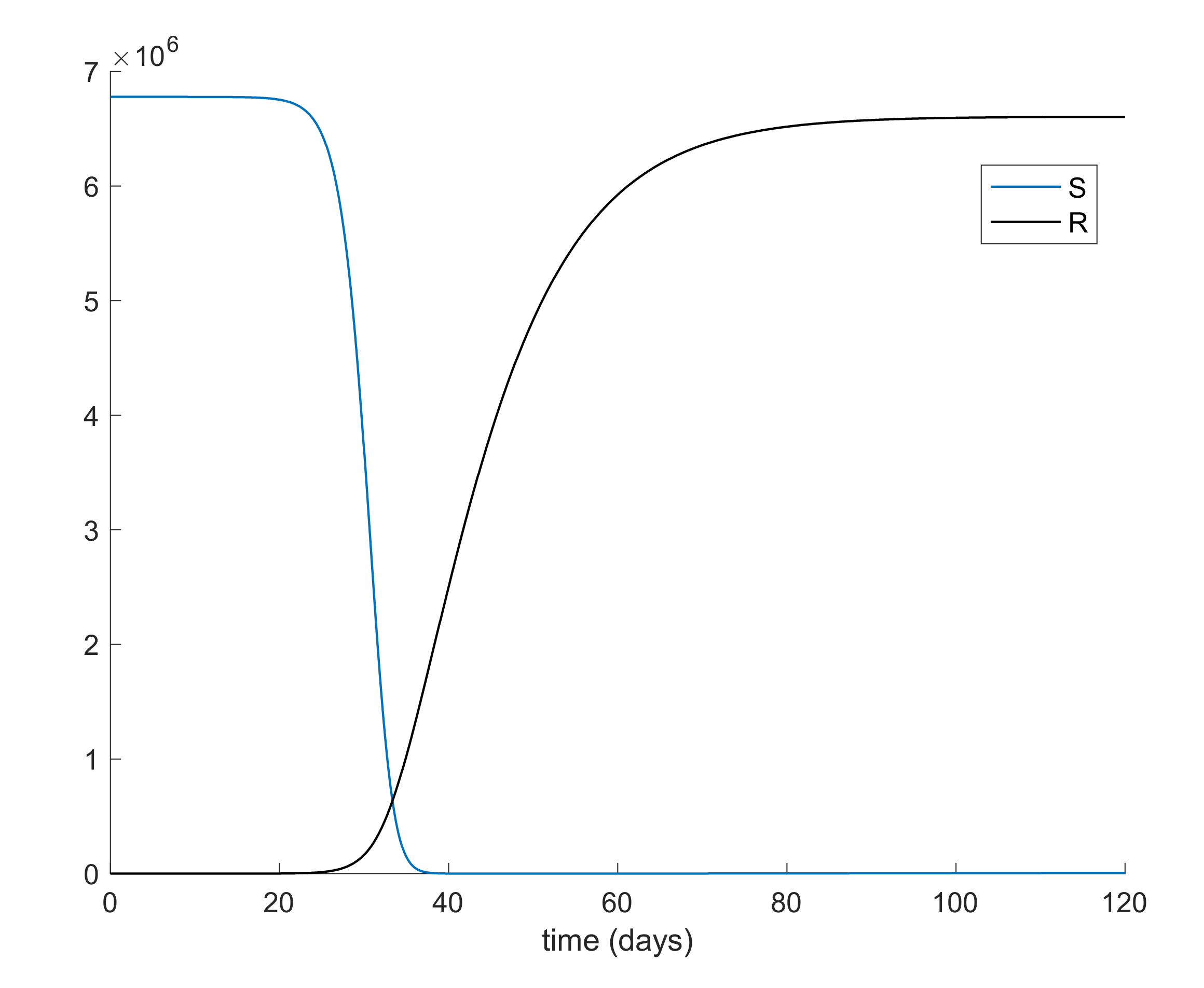
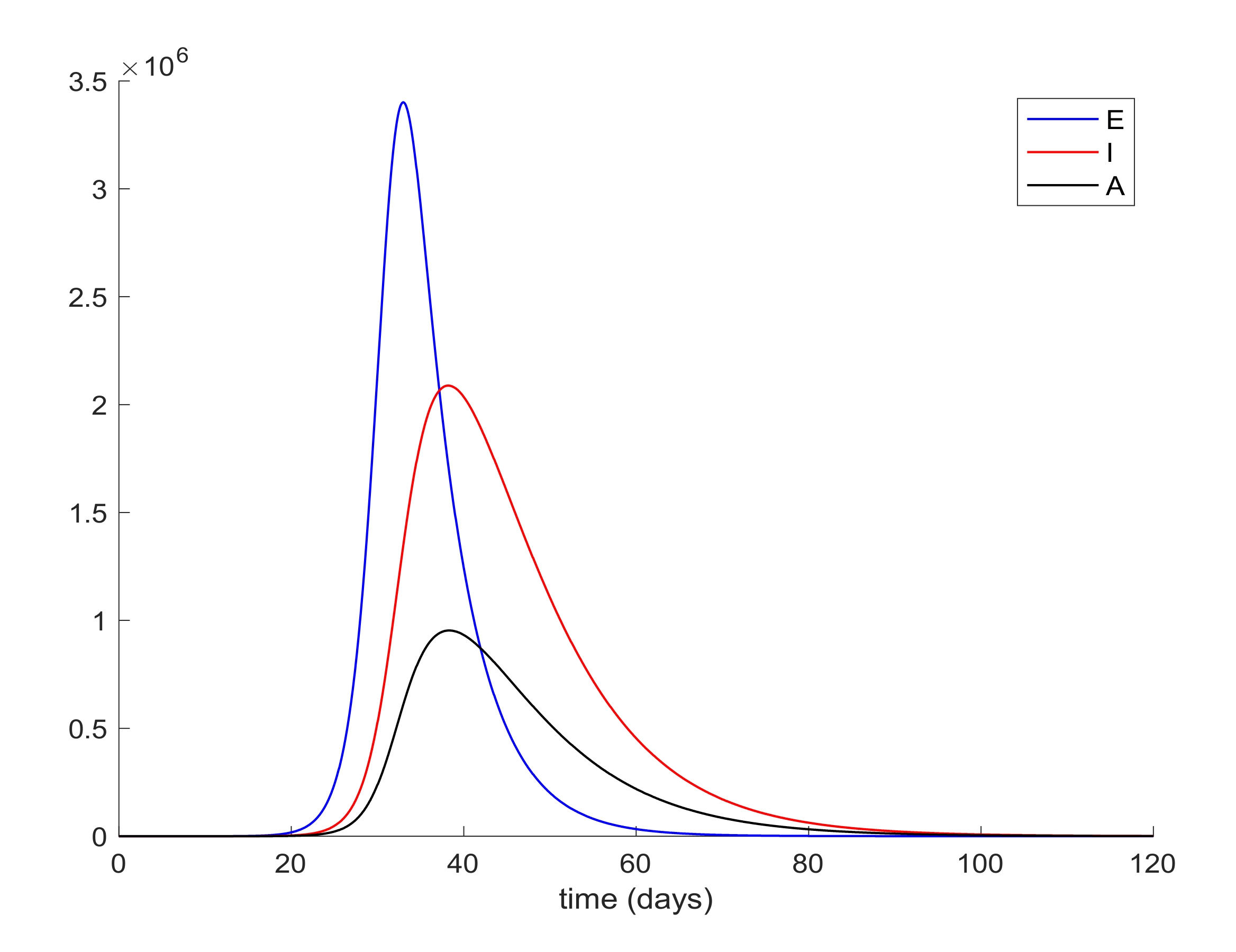
From Table 2, it can be concluded that simulation starts with the total population being susceptible and a single exposed case. Figure 1 and Figure 2 display the evolution of all populations in the absence of control actions. It is deduced from Figure 1 that the spreading of the disease would end up affecting the total population if no control action was taken, as similarly concluded in Reference [45].

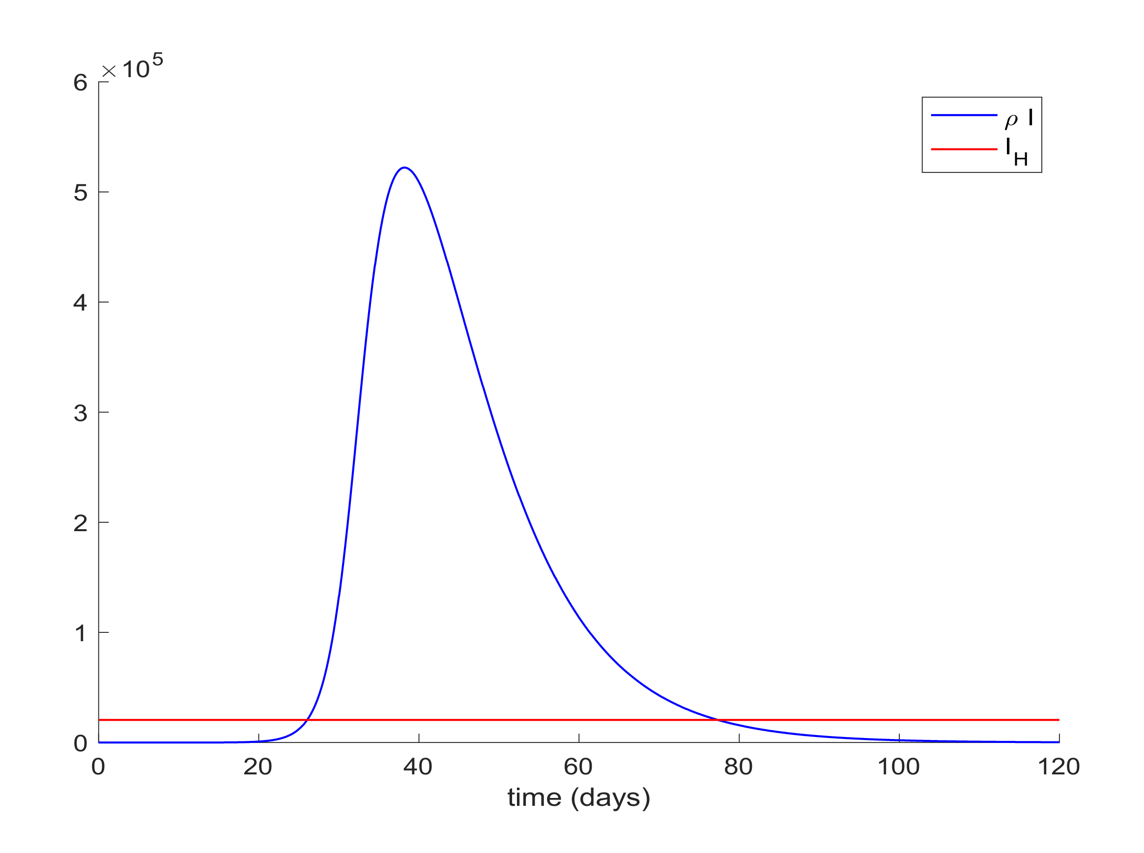
It is also observed in Figure 2 the large number of infected people, I, attained at the infection peak. Such a large number of infected people would definitely overflow the hospital available resources. In order to avoid this situation a quarantine policy will be applied to control the infection spreading. According to [50], it will be considered that the average percentage of infectious cases that require hospitalization is 25%. Thus, the hospital management objective is set as $\rho I(t)=0.25I(t)\le I_H(t)$, where $I_H(t)$ denotes the maximum number of available resources. In the Madrid region, the number of available hospital beds is 20,516, [51], so that the management of hospital resources imply that the constraint $I_H(t)$ should be satisfied for all time. This upper-bound is constant since it is the number of installed beds in the health system before the outbreak of the pandemic, which should not be outnumbered by using the proposed control measurements. 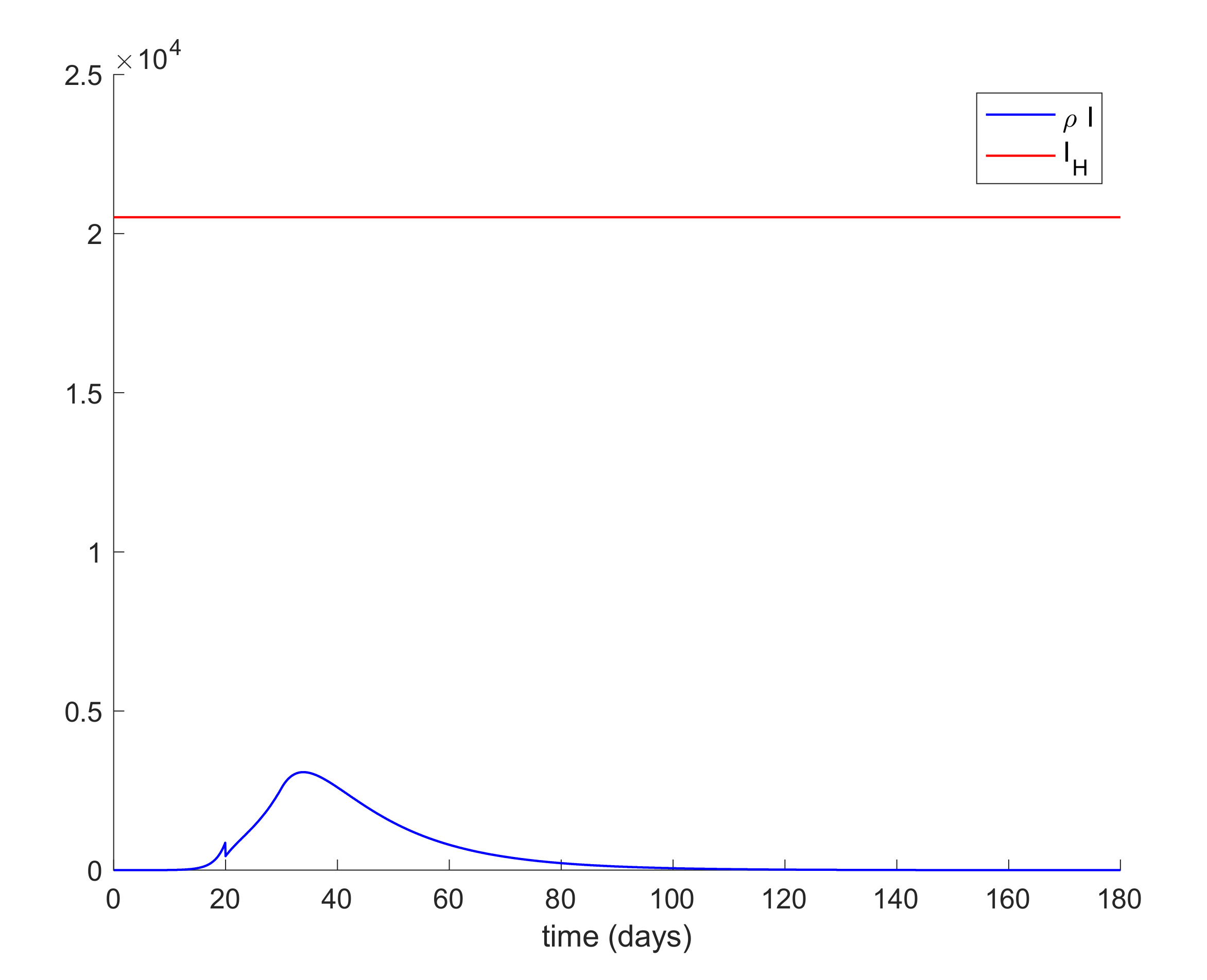This situation is depicted in Figure 3 where it is shown that the hospitalized cases may exceed the number of available beds.

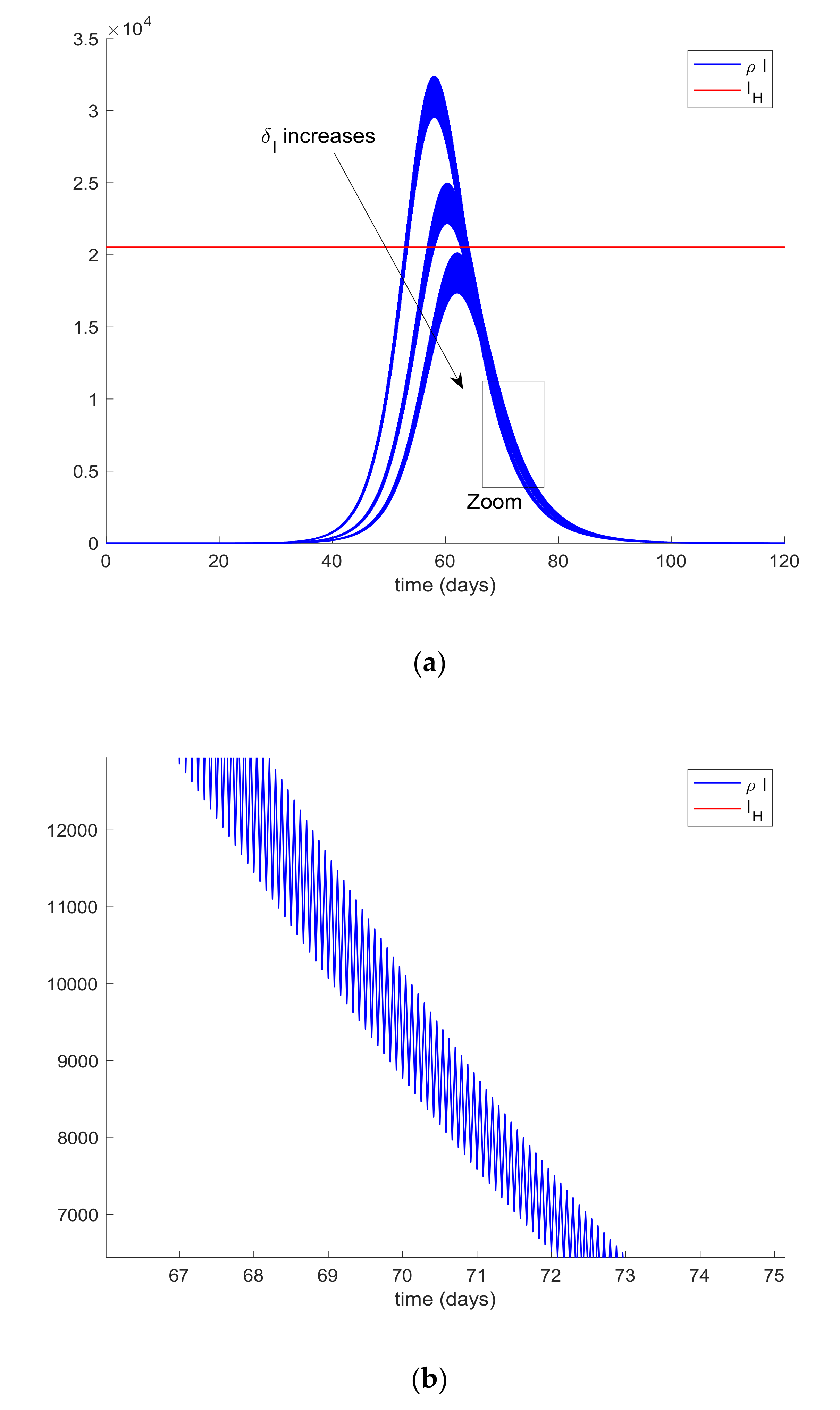
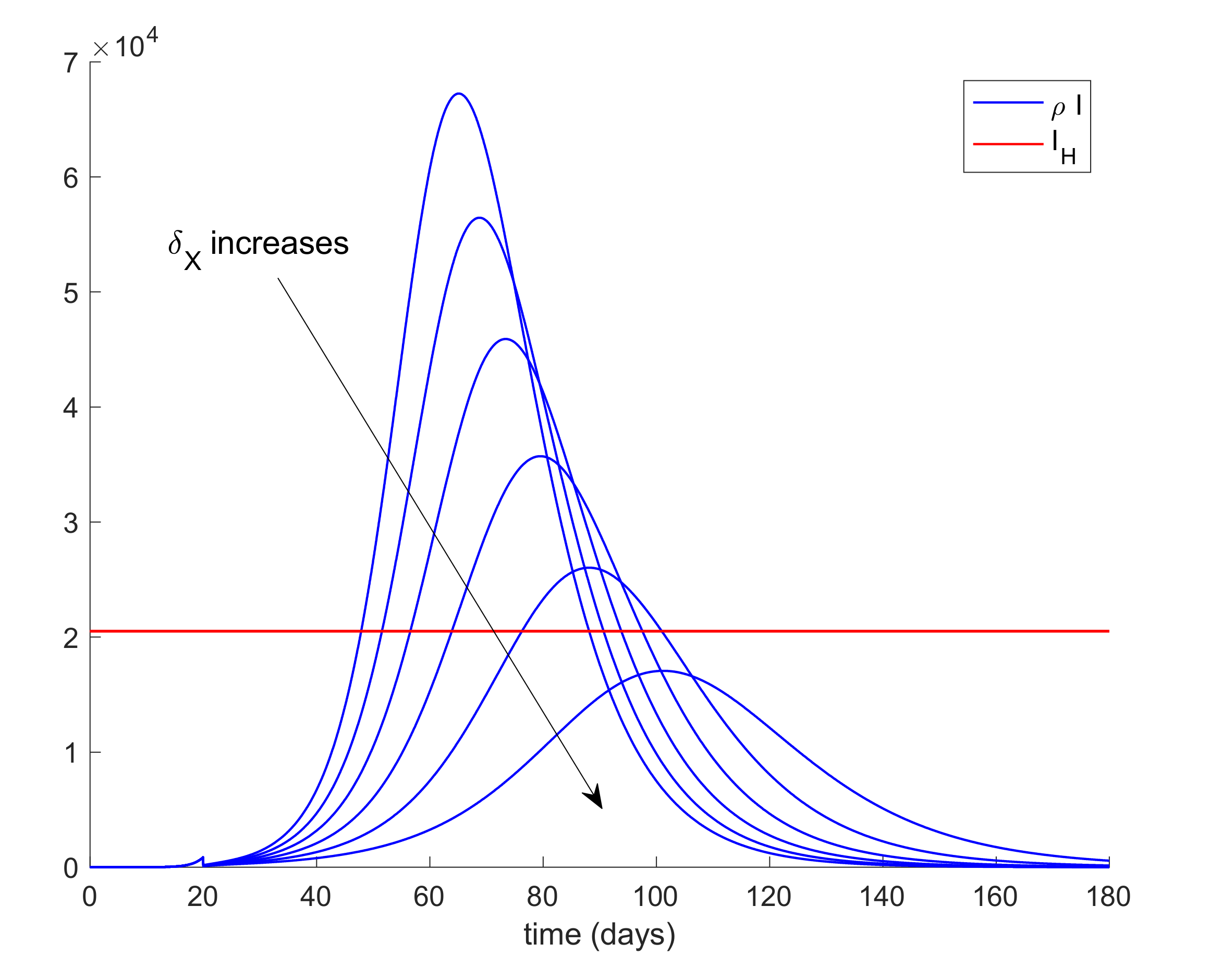
In order to achieve the hospital management objective, quarantine on different populations will be applied. Therefore, the population of infectious cases is assumed t be quarantined (isolated) at different percentages twice per day. This means that every 12 h, a percentage of the infectious population, I, is removed from this compartment due to the fact that they will be isolated and they will no longer spread the infection. Since clinical symptoms may be detected, this population can be quarantined independently from the other ones. Thus, Figure 4 shows the effect of this “isolation of cases” policy. In this way, Figure 4a displays the hospital management objective and the obtained infectious curves for different values of δ_I ranging from 0.16 to 0.24, so that the percentage of isolated infections range from 16% to 24%. Figure 4b also shows the effect of the impulsive action on the infectious evolution.

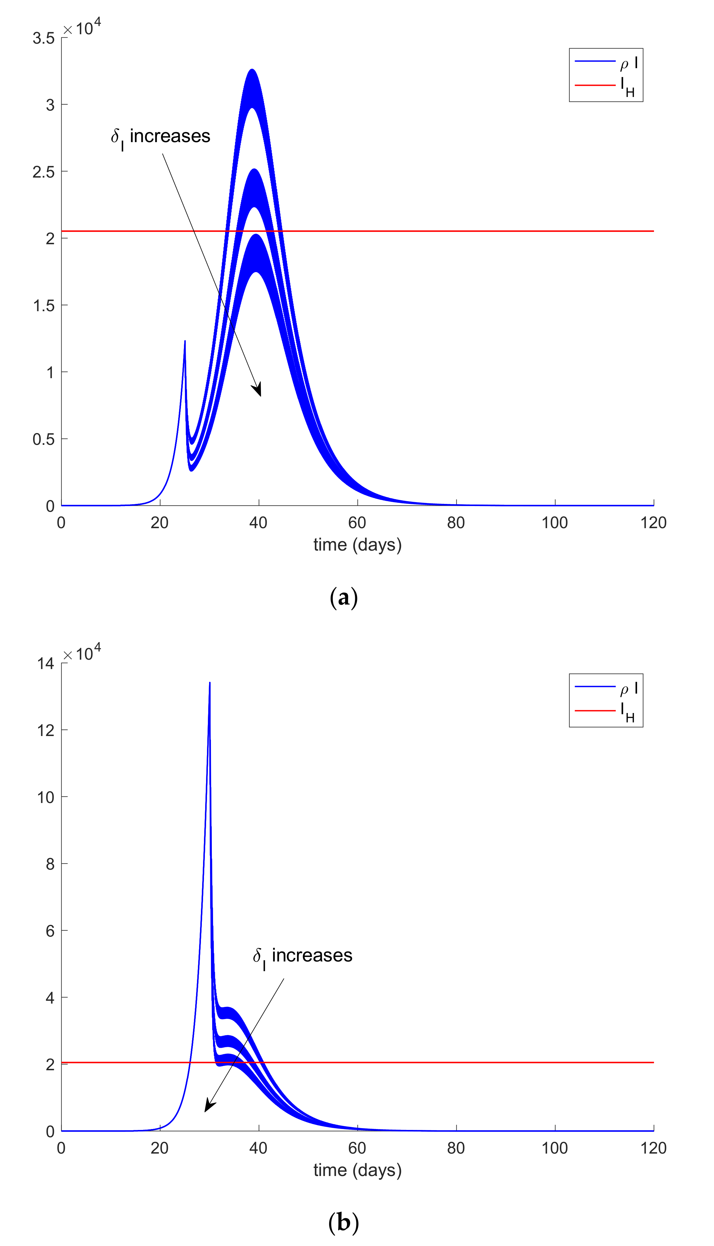
Figure 4 is obtained by assuming that the infectious cases are isolated from the first day of simulation. However, the first day of quarantine (isolation) application may be delayed by a number of days (implying that cases are not isolated and they can still spread the infection for more days) due to several reasons. In this case, the results depicted in Figure 5 are obtained for the same values of δ_I as before (from 0.16 to 0.24). Thus, Figure 5a displays the evolution of infectious cases when the isolation of cases policy starts 25 days before the first exposed case appears while Figure 5b displays the infectious evolution when the isolation policy starts 30 days after. The isolated individuals are removed from the I -compartment.

It can be deduced from Figure 5 that the hospital objective may still be accomplished if the quarantine policy is not delayed too much while, if the delay in the isolation application exceeds a certain threshold, then the hospital objective may not be satisfied. Consequently, it is revealed as crucial to isolate the cases as soon as possible. The limit value for the quarantine percentage that allows fulfilling with the hospital objective at all time points can be calculated by trial-error simulation by using a search algorithm such as Algorithm 1 discussed in Section 2 or by using Equations (61)-(66) evaluated at quarantine application time instants. In this case, simulations for different values are performed to analyze the effect of changing the quarantine percentage procedure that, in turn, allows finding its limit value. On the other hand, Figure 6 displays the evolution of the infectious and hospital beds threshold when a quarantine on the general population is applied at day 20 after the first exposed individual is introduced in the population. This situation is modeled as the reduction of the same percentages of individuals from all populations at day 20. This may be the general situation when a universal lock down is decreed as it was the case of Spain. Therefore, the values of δ_S = δ_E = δ_I = δ_A range between 0.8 and 0.9, which implies that the quarantine involves up to 90% of the whole population. It is observed in Figure 6 that the application of quarantine reduces the peak of infectious cases with respect to not taking any measure but, depending on the percentage, may not be enough to achieve the hospital objective. 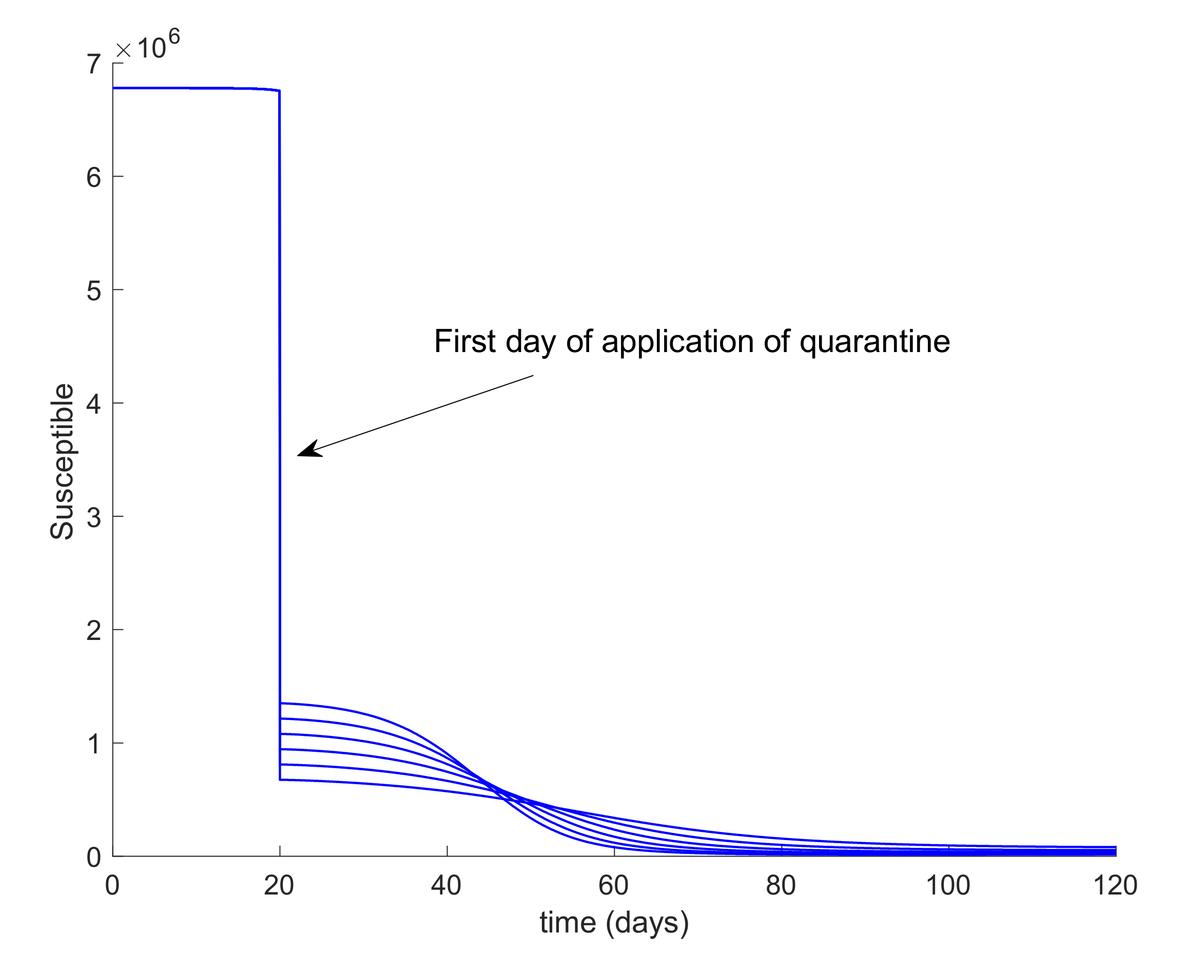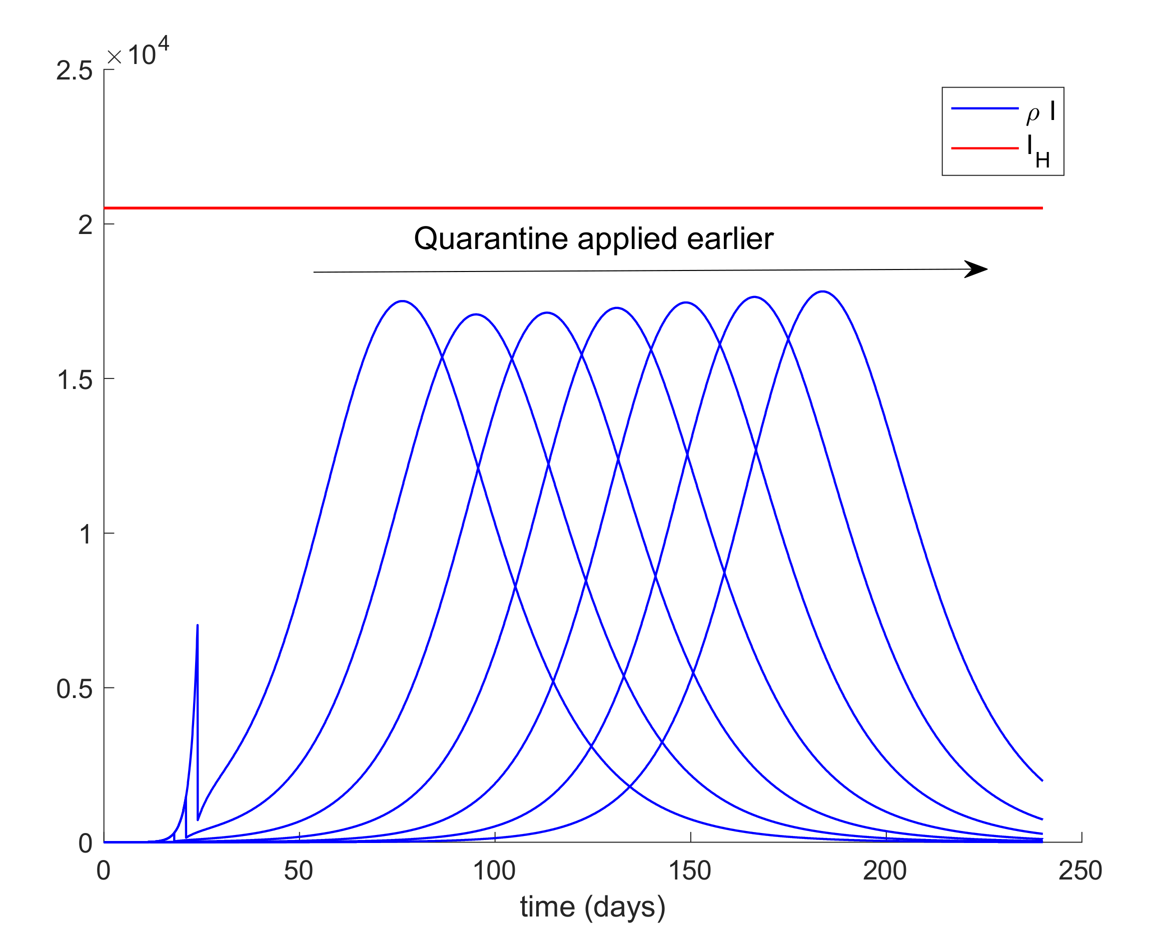Figure 7 displays, as an example, the abrupt change on the susceptible when the quarantine is applied at day 20. Furthermore, Figure 8 displays the change in the evolution of the infectious cases when quarantine is applied at different starting times. Thus, we fix δ_S for all populations and the day when quarantine is applied ranges from 3 to 24 days after the first exposed is introduced in the population. The fact for applying quarantine earlier moves the peak to the right but does not change its value. Therefore, when the quarantine is applied to such a large percentage of population, the time of application is not that crucial. In addition, it is revealed to be more appropriate for early detection and isolation of cases than the quarantine of a large percentage of general population since it allows attaining the hospital management objective without locking down a large amount of individuals.

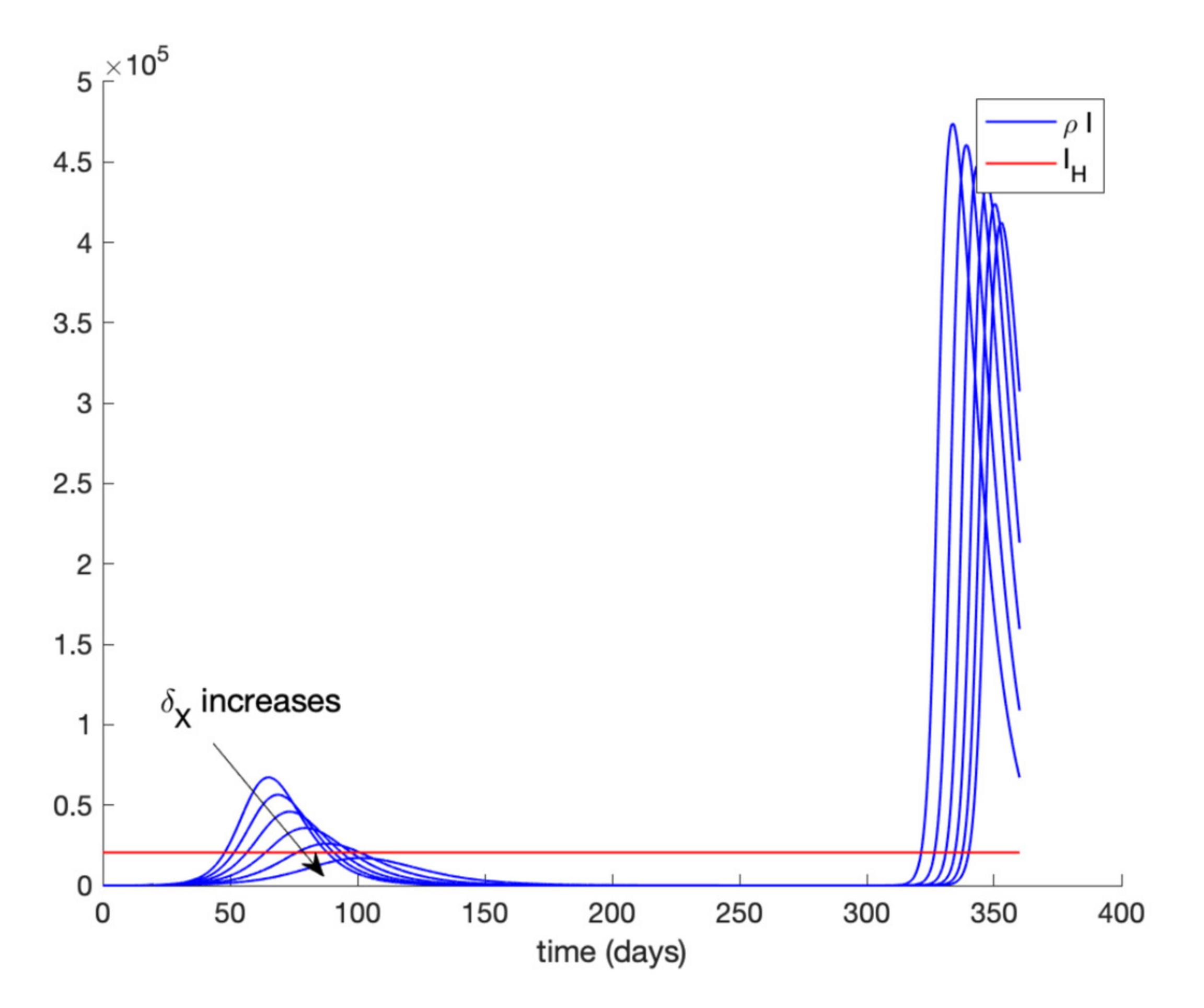
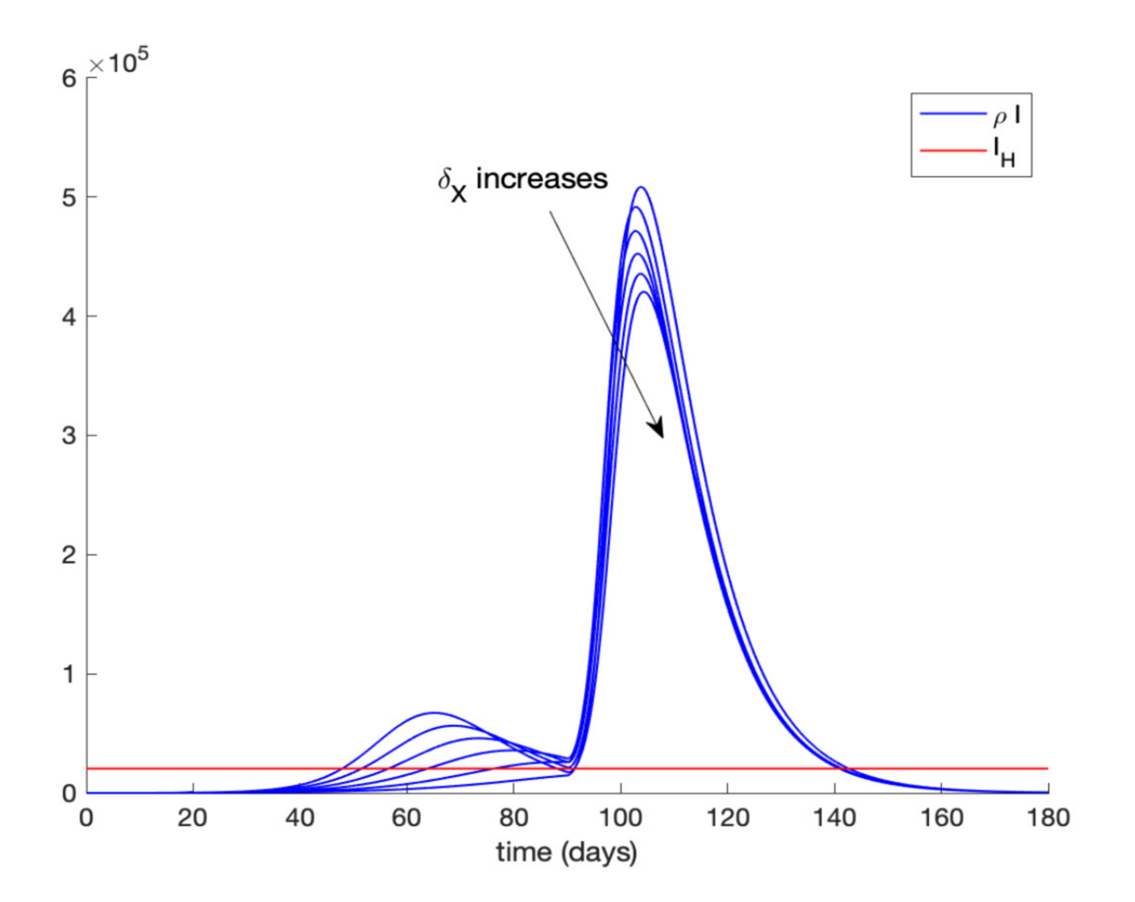
In addition, Figure 9 displays the evolution of infectious cases when quarantining 80–90% of the entire population is ordered at day 20 and relaxed at day 90 while Figure 10 shows the infectious cases when quarantine is lifted at day 300. In all these cases, all quarantined populations are added to the susceptible population once quarantine finishes. It is deduced from Figure 9 and Figure 10 that, when quarantine is lifted, the number of infectious cases rebounds (end exceeds the hospital availability threshold) no matter how long quarantine had been maintained. Thus, the sole application of a general quarantine is not a sufficient control action to deal with the infection spreading since rebounding may occur at the end of quarantine. 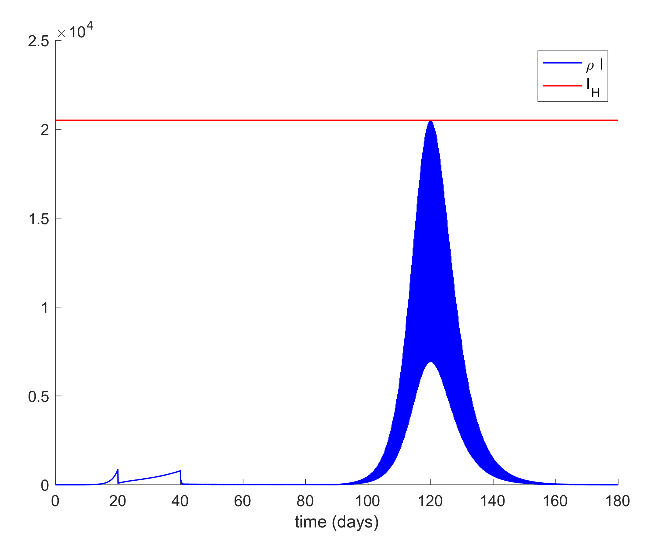Figure 11 shows the effect of isolating 70% of infectious individuals every 6 h after day 40 when a general quarantine for 90% of the population is decreed from day 20 to day 90. It can be concluded from Figure 9, Figure 10 and Figure 11 that an important measure is the early detection and isolation of cases in order to prevent new outbreaks once a situation of quarantine is relaxed.

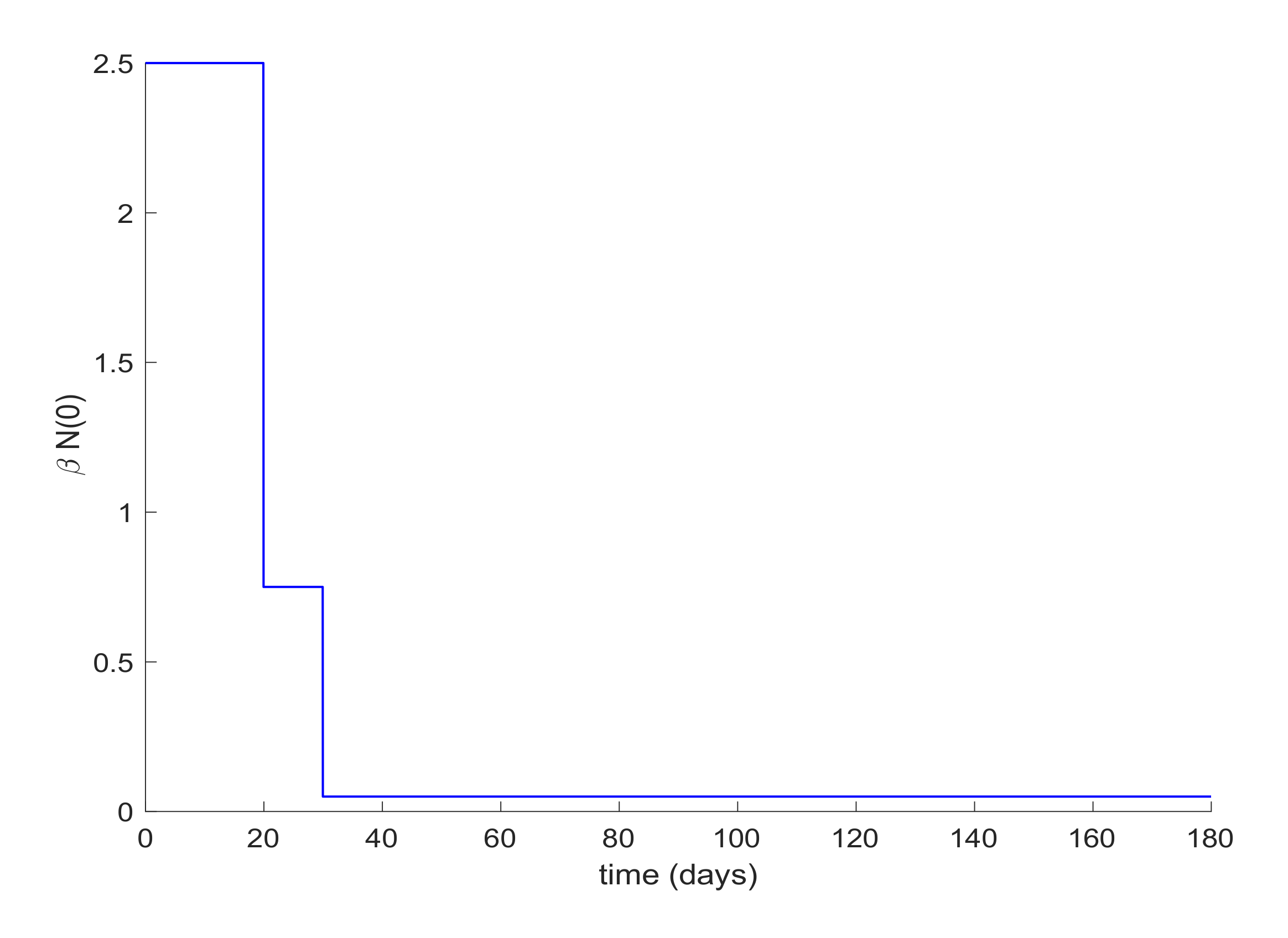
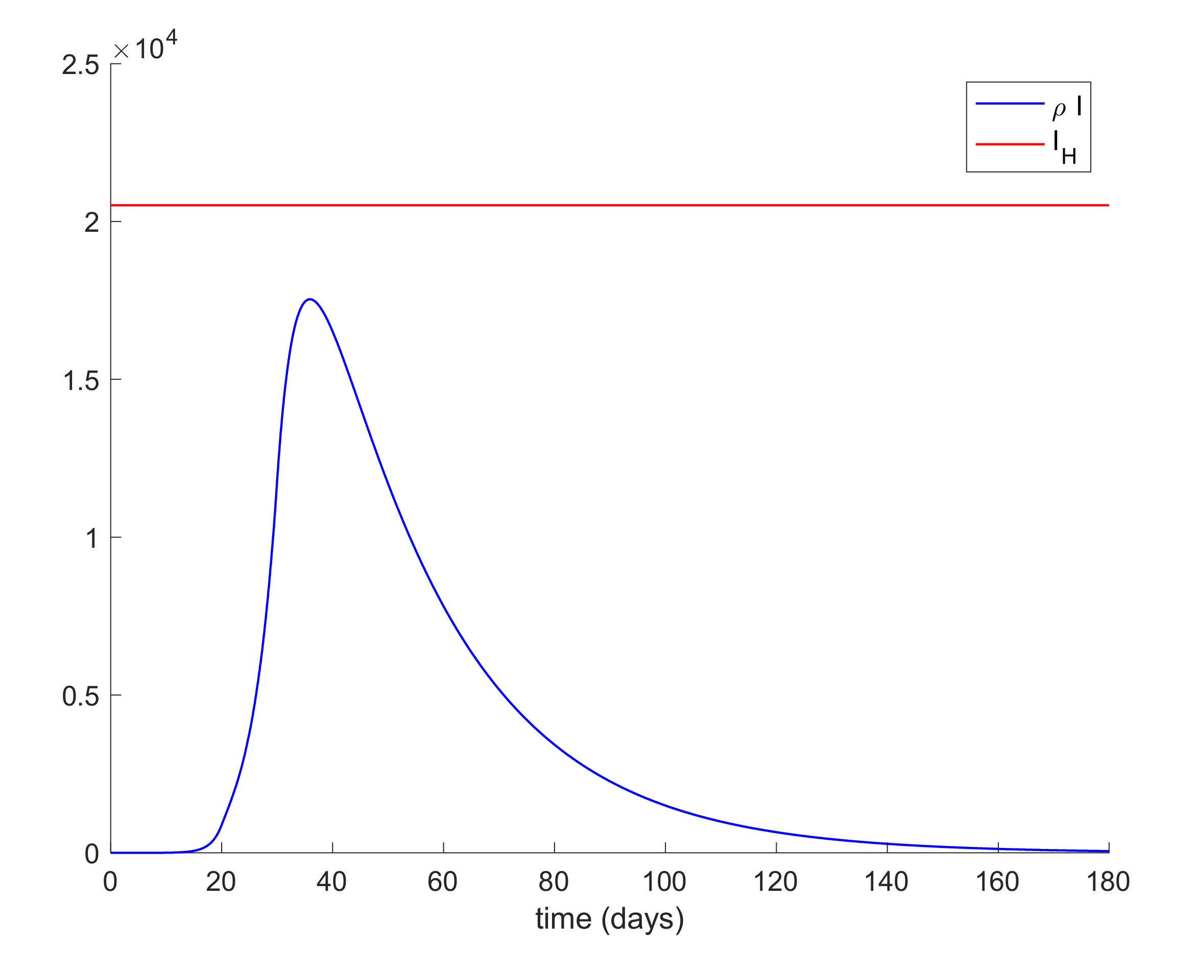
Lastly, quarantine is commonly implemented with social distancing measurements. Social distancing has the effect of reducing the infectivity factor, $\beta$. This factor can also be reduced due to the quarantine application discussed before. Therefore, the last simulation will deal with the case when $\beta$ is a piecewise constant function. In this way, the value of $\beta$ displayed in Figure 12 is proposed for simulation. Figure 13 depicts the evolution of the infectious cases with the displayed piecewise constant beta and no other control action. It is observed in Figure 13 that the hospital requirement is fulfilled in this case. Thus, an early reduction of the infectivity rate is crucial to control the infection spreading. Figure 14 shows the effect of joining a reduction of the infectivity rate with quarantine of 50% of the entire population from day 20. It can be concluded that the joint effect is able to attain the hospital requirement in an easier way than by using a single method.

It can be pointed out that current data regarding Covid-19 exhibit high variability between outbreaks and places and many of them include many inconsistencies such as a negative number of deaths in order to regularize incorrectly informed data. It was very common to give erroneous data at the beginning of the infection outbreak since only the seriously infected individuals were tested. Therefore, those with unserious symptoms and those being asymptomatic were not tested. Thus, the confrontation of the model with real data will require an important work of data gathering and analyzing. Therefore, the total number of total infectious cases at any time of the infection evolution can be roughly estimated by the number of deaths caused by the illness with the estimated proportion of 1%-1.5% of deaths from all of the infectious individuals in accordance with recently reported estimations. Basically, the model adequacy analysis could be performed by comparing the actual number of deaths and ICU hospitalized patients from the results obtained from the model. This process will definitely require an appropriate definition of cases and the review of previously informed data. On the other hand, the transmission rate of the symptomatic and asymptomatic infectious subpopulations can be updated through from the corresponding given data by the health system. The remaining parameters of Table 1 can be updated from medical data on hospital records and testing records on populations. This methodology may be useful to adjust the model parameterization from recorded data on the disease evolution.

6. Conclusions

This paper has considered the problem of partial or total quarantines of the susceptible and the susceptible and infectious populations of both a simple SIR model and a more general SEIAR model with mortality and demography. Such a model incorporates the asymptomatic infectious subpopulation to the usual SEIR models. The proposed model is studied under either partial or total quarantines of some or of all of the subpopulations in order to satisfy prescribed hospital availability requirements on bed disposal and other necessary treatment means. The quarantined fractions of one or various involved subpopulations can be mutually distinct. In this way, the total confinement becomes a particular case of quarantine intervention. The hospital objective to be fulfilled is being prescribed through time as a monitored design constraint on the seriously infectious subpopulations, which needs hospital care. Such a subpopulation is assumed to be a fraction of the total infectious individuals while the objective management establishes that their numbers should be kept below a prefixed absolute upper-boundary, which cannot be violated. Some simulated numerical examples are also discussed by using modelling parameterizations related to the current COVID-19 pandemic. Those simulations corroborate that quarantine interventions with enough anticipation related to the pandemic outbreak and the appropriate identification of cases are efficient tools for the fulfilment of required hospital management objectives.