The Emergence of Chaos in Quantum Mechanics

Abstract

Nonlinearity in Quantum Mechanics may have extrinsic or intrinsic origins and is a liable route to a chaotic behaviour that can be of difficult observations. In this paper, we propose two forms of nonlinear Hamiltonian, which explicitly depend upon the phase of the wave function and produce chaotic behaviour. To speed up the slow manifestation of chaotic effects, a resonant laser field assisting the time evolution of the systems causes cumulative effects that might be revealed, at least in principle. The nonlinear Schrödinger equation is solved within the two-state approximation; the solution displays features with characteristics similar to those found in chaotic Classical Mechanics: sensitivity on the initial state, dense power spectrum, irregular filling of the Poincaré map and exponential separation of the trajectories of the Bloch vector $\mathit{\sigma }$ in the Bloch sphere.

1. Introduction

The theory of chaos gained the role of a new paradigm of Science for explaining a large variety of phenomena by introducing the concept of unpredictability within the perimeter of Classical Physics. Chaos occurs when the trajectory of a particle is sensitive to the initial conditions and is produced by a nonlinear equation of motion [1]. As examples we quote the equation for the Duffing oscillator (1918)

$$m\ddot{x}+\gamma \dot{x}+r{x}^3=F\cos \left({\omega }_{L}t\right)$$

(1)

or its elaborated form

$$m\ddot{x}+\gamma \dot{x}+kx+r{x}^3=F\cos \left({\omega }_{L}t\right)$$

(2)

that are among the most studied equation of mathematical physics [1,2] and, as far as we know, cannot be analytically solved. These equations model complex systems with a huge number of microscopic interactions hidden in the chosen value of the phenomenological parameters $\gamma$, k and r. The equations share a relevant property: ranges of the numerical value of the parameters and of the initial conditions exist, which make the prediction of the final output of the motion useless, since any two trajectories starting from close initial conditions exponentially separate with time. What we are saying is that the study of complex systems, in which the dynamics are only partially known, may require models with nonlinear equations of motions and ensuing emergency of chaos. Only nonlinear systems can lead to chaos although not all nonlinear systems are chaotic. Two trajectories of a physical system in the chaotic regime must be aperiodic, must not intersect in phase space $\{q_i,{\dot{q}}_i,t\}$ for $t<+\infty$ and must exponentially diverge when starting with close initial conditions [3,4]. As far as we know, no general rule is known proving the chaotic nature of a physical system, although an interesting model displaying these characteristics can be constructed [4] where such a proof exists.

Almost by definition, Quantum Mechanics lays its foundation in the study of experimental unpredictability by describing the outcome of a measurement act with its probability.

However, the evolution of the wave function is ruled by the linear Schrödinger equation that permits the superposition principle: the sum of two different solutions is still a solution. Moreover, in Quantum Mechanics the concept of trajectory needs to be handled with care since it cannot be seen in the same way as in Classical Physics: determined by the knowledge of initial position and velocity, although a proxy of the classical concept may be recovered by use of the Ehrenfest theorem. These characteristics forbid the observation of chaos in the same fashion as in Classical Physics: the time evolution of the wave function is predictable. Thus, the quest for chaos within Quantum Mechanics requires some slight modification of paradigm.

However, also in Quantum Mechanics, when dealing with many interacting quantum particles or complex systems, nonlinear equations are found. As examples, they are obtained in the self-consistent Hartree-Fock method [5] or in the study of the motion of an excitation along one-dimensional molecular chains [6,7]. In principle these equations might display chaotic behaviour when opportune physical parameters are chosen. We may say that nonlinearity in these approaches is of extrinsic origin for it lays its ground on the linear Schrödinger equation and appears as a way to deal with complex systems in which dynamics are only partially known.

Indeed, examples of chaotic comportment are present in Quantum Mechanics. Experiments on the ionization of hydrogen atoms in a microwave field [8,9] showed a dependence upon the intensity of the driving field, which can be explained by the insurgence of chaos. Moreover by using Bohm’s formulation of the theory one can obtain a trajectory-based representation of a quantum mechanical system completely equivalent to the one based on the wave function obtained from the linear Schrödinger equation [10,11,12]. These trajectories manifest chaotic behaviour [11,13,14,15,16,17]. The reason for this feature is that in Bohm mechanics, the quantum evolution assumes a hydro-dynamical form, which has chaotic solutions. The surprising point in Bohm’s picture of Quantum Mechanics is that the underlying chaos does not emerge in the standard linear Schrödinger picture as if, apparently, washed out in the transition to the standard form of the theory. This, we believe, is as yet a not well understood issue, requiring in-depth analysis.

From the ontological point of view, the linearity of the Schrödinger equation has been questioned by the introduction of an intrinsic nonlinearity term in the Hamiltonian [14,18,19,20,21]. In this paper, we explore two different nonlinear Hamiltonians; they may be considered as the model of collective and complex interaction much in the same way as the rationale for Equations (1) and (2) otherwise they can be seen as a possibility for a basic nonlinear Schrödinger equation.

Chaos is an asymptotic effect and might appear after a long period of time; it is important in this condition to introduce an external field, which enhances the dynamics of the system and forces chaos to emerge through cumulative effects. Thus, in this paper, we study the evolution of a quantum system governed by a nonlinear Schrödinger equation and driven by a resonant laser of angular frequency ${\omega }_L$; in fact, resonance is the most efficient coupling between radiation and matter and mostly apt to cause rapid modifications of the dynamics.

If a nonlinear Hamiltonian rules the time evolution of a system, then the final wave function contains this information and leads us to the question if the information can be extracted from the measurement of opportune final physical quantities. We believe that a positive answer to this question would be important as it would relate final measured quantities to initial measured quantities without a detailed analysis of the time evolution of the wave function.

To provide a reliable answer to the question is an important goal. We believe that the results of this paper suggest that a positive answer is possible. Of course this is not, as yet, the definitive statement, and efforts and researches are still needed.

Before entering the full description of the theory, we should ask ourselves on the necessity of looking for a fundamental presence of nonlinearity and insurgence of chaos in Quantum Mechanics for, at the moment, it does not appear a cogent reason for it. In Classical Mechanics, chaos is present and the impression that it rules the evolution of the majority of phenomena is unavoidable; then why does it appear to be marginal in Quantum Mechanics since the correspondence principle asks for it? Actually, to challenge linearity could also require the challenging of the corresponding principle which, after all, was formulated when chaos was little more than Poincaré’s intuition. Nonetheless, curiosity compels the investigation of the issue.

2. Two Routes to Chaos

The presence of a laser field to drive quantum systems introduces a wealth of phenomena, which are of interest in fundamental and applicative physics. Among these phenomena, the process of high order harmonic generation (HHG) is relevant here; it occurs when a quantum object driven by the laser field at frequency ${\omega }_L$ irradiates electromagnetic radiation in which the spectrum is formed by a very large plateau of odd multiples of ${\omega }_L$; the absence of even harmonics being motivated by symmetry properties of the Hamiltonian. For simplicity sake, in what follows, we refer to the systems as an atom. The radiation is the result of a strong acceleration of the atomic charges, which is highly nonlinear with the laser-atom interaction energy $U_0$ and provides a benchmark for testing nonlinear phenomena and ground to new high frequency lasering devices [22,23,24]. Moreover, the radiation, produced by the field where the active charges are present, carries relevant information of the local status of the charges; thus, HHG can be an efficient spectroscopic tool for observing features otherwise undetectable [25,26,27]. The purpose of this paper is to exploit the fast modification of the wave function of the atom to explore a form of nonlinearity different from the one above mentioned and due to a dependence of the quantum Hamiltonian upon the wave function of the system. We show that the presence of the laser makes apparent a chaotic quantum behaviour.

To recognise chaotic behaviour, the Poincaré map is useful. The nature of a motion driven by a force with period T is conveniently studied by plotting in the configuration space the stroboscopic point

$$\mathit{P}\left(nT\right)=\left(q_1\left(nT\right),q_2\left(nT\right),\dots ,{\dot{q}}_1\left(nT\right),{\dot{q}}_2\left(nT\right),\dots \right)$$

(3)

with integer n; the distribution of the points gives qualitative information on the chaotic nature of the problem [1]. The best, quantitative, method for diagnosing chaos is to compute the Lyapunov exponent $\lambda$. It provides the degree of divergence of two chaotic orbits with a nearby starting point [2,28]; if $D\left(t\right)$ is the distance between the orbits at a time t, then $D\left(t\right)=D\left(0\right)2^{\lambda t}$. If $\lambda >0$, then the motion is chaotic.

We consider a laser driven quantum system in which the evolution is governed by a nonlinear Hamiltonian $\widehat{H}\left(t\right)$; the nonlinearity might have intrinsic (i.e., fundamental) or extrinsic (i.e., external) origin. Coherently with the resonant assumption, we adopt a two level scheme for the atom, scheme which was used in the past for similar purposes [29]; thus the equation of the system is

$$i\hslash \dot{\mathit{c}}\left(t\right)=\widehat{H}\left(t\right)\mathit{c}\left(t\right)$$

(4)

with the nonlinear Hamiltonian $\widehat{H}\left(t\right)$ a $2\times 2$ matrix and

$$\mathit{c}\left(t\right)=\left(\begin{array}{c}{c}_0\left(t\right)\\ c_1\left(t\right)\end{array}\right).$$

(5)

Many forms for the nonlinear Hamiltonian can be conjectured and often a dependence upon the square modulus of the wave function [18,30] is assumed. Here we wish to explore a dependence upon the phase of the wave function that might describe the de-coherence produced by a sudden interaction between the active atom and the environment.

We introduce two Hamiltonians. The first Hamiltonian is

$${\widehat{H}}_1=\frac{\hslash }{2}\left(\begin{array}{cc}-{\omega }_0& 2{\varpi }_1{c}_0^{\ast }{c}_1\\ 2{\varpi }_1{c}_0{c}_1^{\ast }& {\omega }_0\end{array}\right)+U_{0}f\left(t\right)\left(\begin{array}{cc}0& \sin \left({\omega }_{L}t\right)\\ \sin \left({\omega }_{L}t\right)& 0\end{array}\right)$$

(6)

which explicitly contains the phase difference between the two bare eigenstates through $c_0\left(t\right)c_1^{\ast }\left(t\right)$. In the absence of a laser in this Hamiltonian, the two levels remain stationary: if $c_0\left(0\right)=0$ or $c_1\left(0\right)=0$ then the Hamiltonian is diagonal and there is no free decay from upper to lower level.

The second Hamiltonian is

$${\widehat{H}}_2=\frac{\hslash }{2}\left(\begin{array}{cc}-{\omega }_0& 2{\varpi }_2{e}^{i({\varphi }_1-{\varphi }_0)}\\ 2{\varpi }_2{e}^{i({\varphi }_0-{\varphi }_1)}& {\omega }_0\end{array}\right)+U_{0}f\left(t\right)\left(\begin{array}{cc}0& \sin \left({\omega }_{L}t\right)\\ \sin \left({\omega }_{L}t\right)& 0\end{array}\right)$$

(7)

where ${\varphi }_0\left(t\right)$ and ${\varphi }_1\left(t\right)$ are the phase of the ground and the excited state. In this way, the nonlinear term depends only upon the relative phases of the states. The value of the nonlinear parameters ${\varpi }_n$ does not depend upon the laser. In both Hamiltonians, the laser-atom interaction energy is the term containing $U_0$.

Moreover, in this delicate field at issue, it is of paramount importance to make clear our operational steps to define as chaotic the evolution of the atom.

(i)

For our purposes, the first, fundamental step is to plot selected final physical quantities as a function of initial physical quantities. By inspection we infer if they can be caused by a chaotic behaviour. Of course we are aware that this is a qualitative method that can lead to misjudgements.

(ii)

In general, a dense power spectrum of a physical quantity is considered an indication. In our analysis we use the power spectrum of the electric dipole moment, the choice is motivated by the fact that the dipole moment is related to the electromagnetic radiation from an atom.

(iii)

In the search for chaos, the Poincaré section is a very important tool. We use it as a flag of chaos.

(iv)

Since all the previous points provide only a qualitative characterisation of chaos, as a final step we calculate the Lyapunov exponent of the orbits of the Bloch vector.

2.1. First Hamiltonian

For the first Hamiltonian, we adopt the following value for the physical parameters: the energy separation between the two levels is $\hslash {\omega }_0=4$ eV while the laser photon is taken $\hslash {\omega }_L=\hslash {\omega }_0/4$ corresponding to a laser optical cycle $T_L\approx 4.1\times {10}^{-15}$ s. The laser pulse has been taken as purely sinusoidal with sudden on–off switching ($f\left(t\right)=1$) with duration $t_f=2^{12}$ optical cycles (oc) corresponding to $t_f\cong 1.6\times {10}^{-11}$ s; the reason of such a long pulse is given by the awareness that chaos might appear after a long time. The laser-atom interaction energy is $U_0=5\times {10}^{-1}$ au. The numerical integration of the nonlinear Schrödinger equation with Hamiltonian (6) has been always carried out with $2^{11}$ integration steps per oc. For physical reasons, the nonlinearity term must be small and is always ${\varpi }_1=1.5\times {10}^{-2}$ au.

An important issue is the free decay time of an excited system, which, for an atom, is of the order of ${\tau }_d\approx {10}^{-8}$ s. Any use of a longer integration time should take into consideration the incoherent mixing of the two states introduced by the decay; in other words, the relation ${\tau }_d>t_f$ should be satisfied. This is the case in the present calculation and leaves room to further increases of the pulse duration. However, physical examples are known with a very long decay time; for example, the radiative life time of ${}^{229}$Th is of the order of ${10}^4$ s [31] while the natural lifetime of the ${}^2{F}_{7/2}$ state of ${}^{171}$Yb${}^{+}$ is of the order of 1 y [32]; both transitions can be coupled with a laser. Of course, such long living states would unburden the experimenter from free decay impediments.

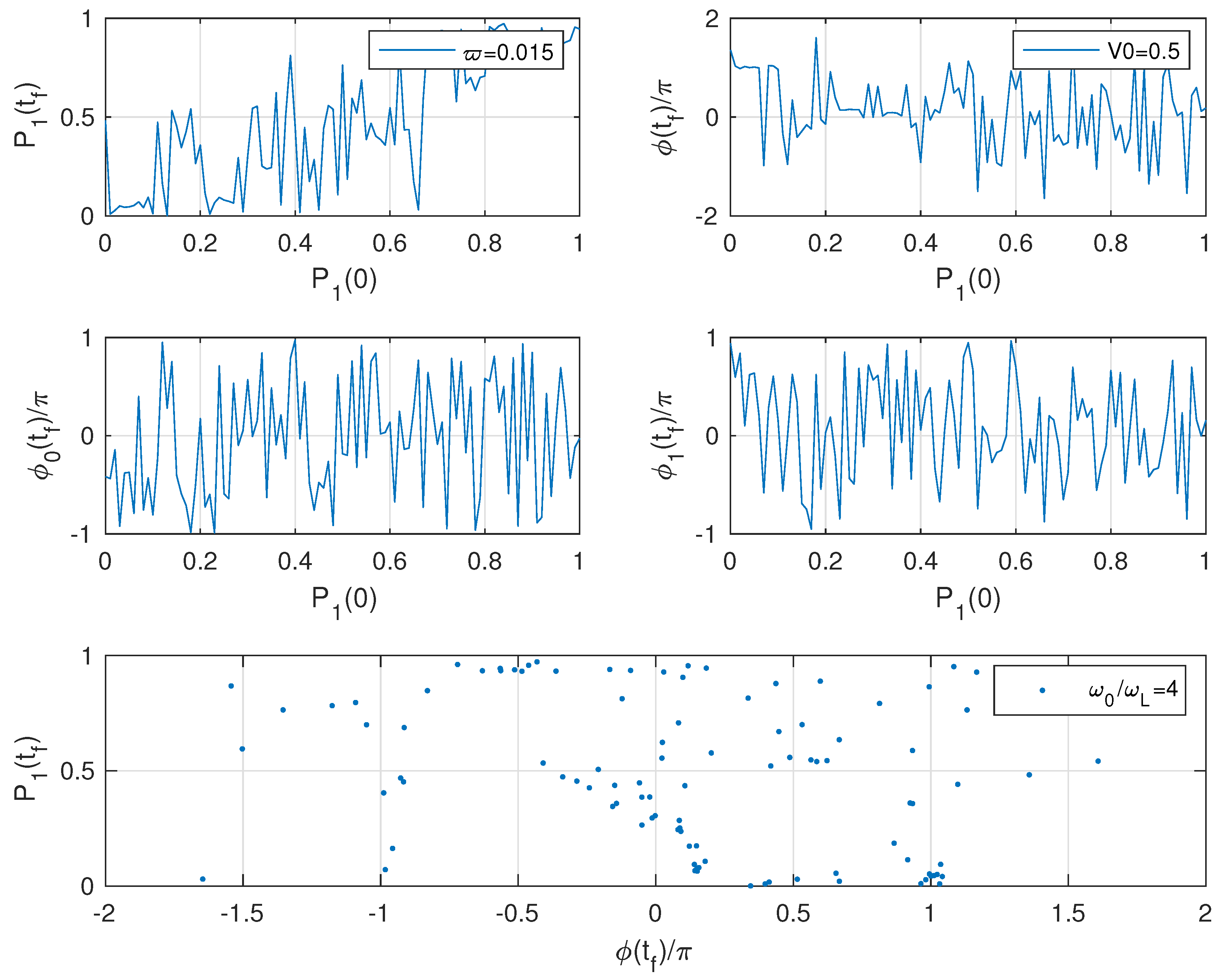
In Figure 1, we plot several final quantities as a function of the initial population of the excited level: no relation appears to exist between the points; this means that the final value of any quantity can be known only after an explicit numerical calculation is performed. According to our scheme, this is a candidate chaotic case.

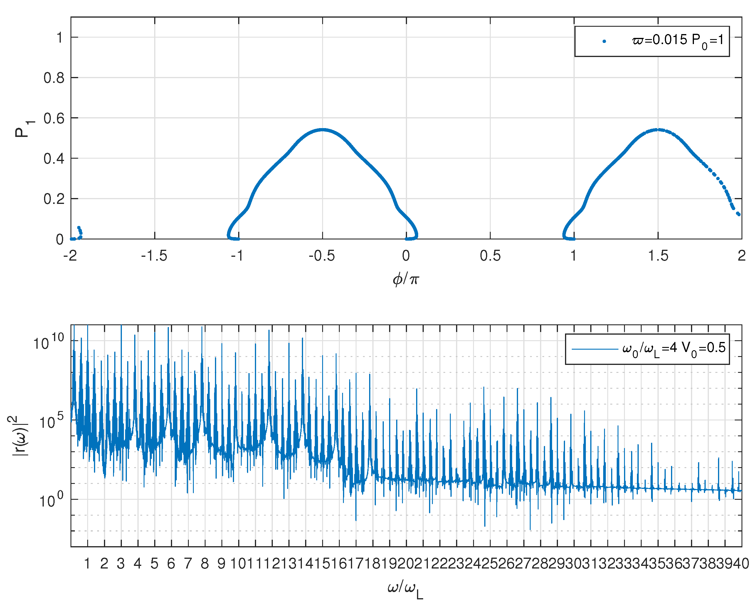
In Figure 2, we show the population of the upper state as a function of the relative phase between the two states; the points are taken at intervals of 1 oc and lie on a regular curve: they are not chaotic. The HHG spectrum is formed of well resolved lines. In Classical Physics, the presence of a broad spectrum in the Fourier transform suggest chaos [2]; this is not the case here: the reason is that the spectrum contains many discrete lines, and the evolution has a quasi-periodic nature. Thus, the first Hamiltonian presents chaotic solutions but suggests care in the choice of the examined quantities.

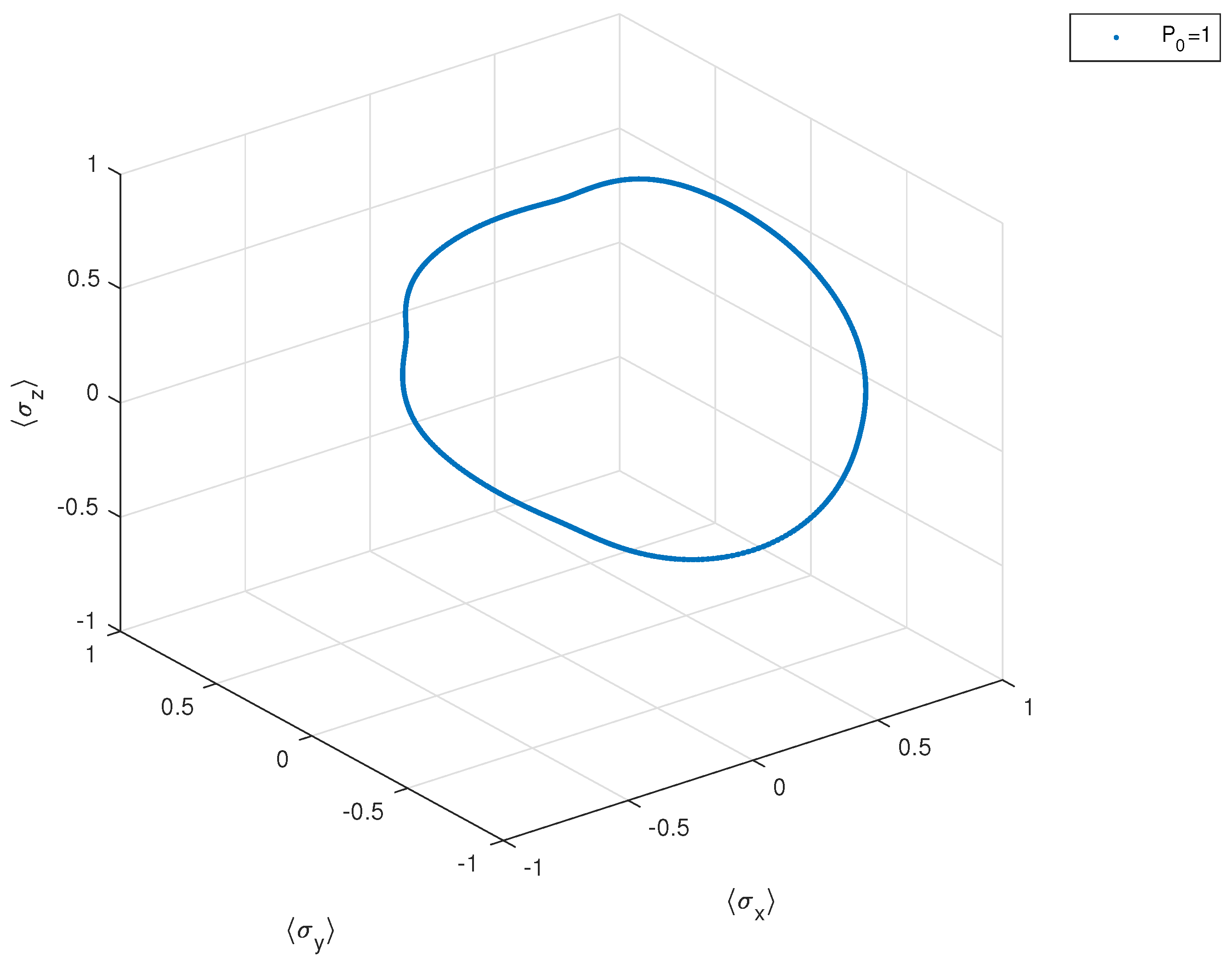
Within the limits of two-state systems, any linear operator can be written as a sum of the Pauli ${\sigma }_n$ and unit matrices. Thus, the three dimensional vector $\mathit{\sigma }\left(t\right)$ with components $\langle {\sigma }_i\rangle \left(t\right)=\langle \mathit{c}\left(t\right)|{\sigma }_i|\mathit{c}\left(t\right)\rangle$ contains all information on the evolution of any observables; therefore, $\mathit{\sigma }$ proves to be an important concept in the detection of quantum chaos. As well known, $\mathit{\sigma }$ is a unit vector lying on the surface of a unit sphere (Majorana or Bloch sphere).

In Figure 3, we plot the three $\langle {\sigma }_i\rangle \left(nT\right)$ when the initial state is the ground one: they are located on a regular curve. No chaotic motion is observed.

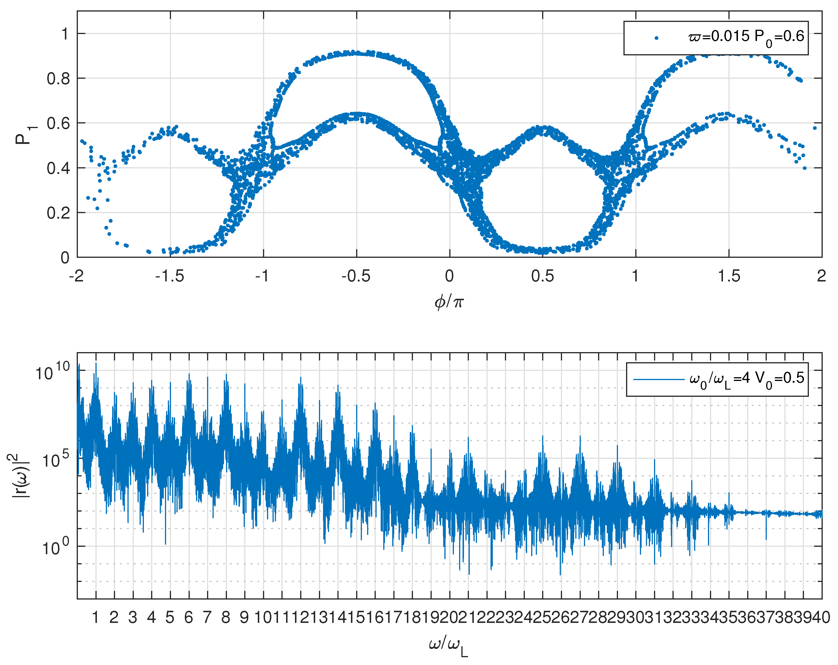
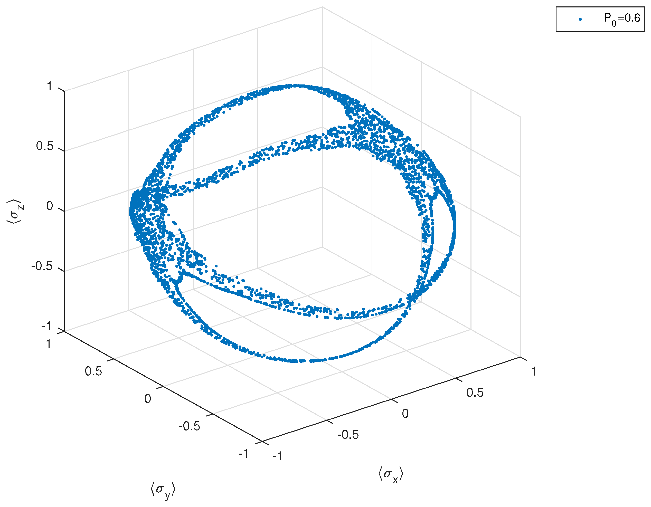
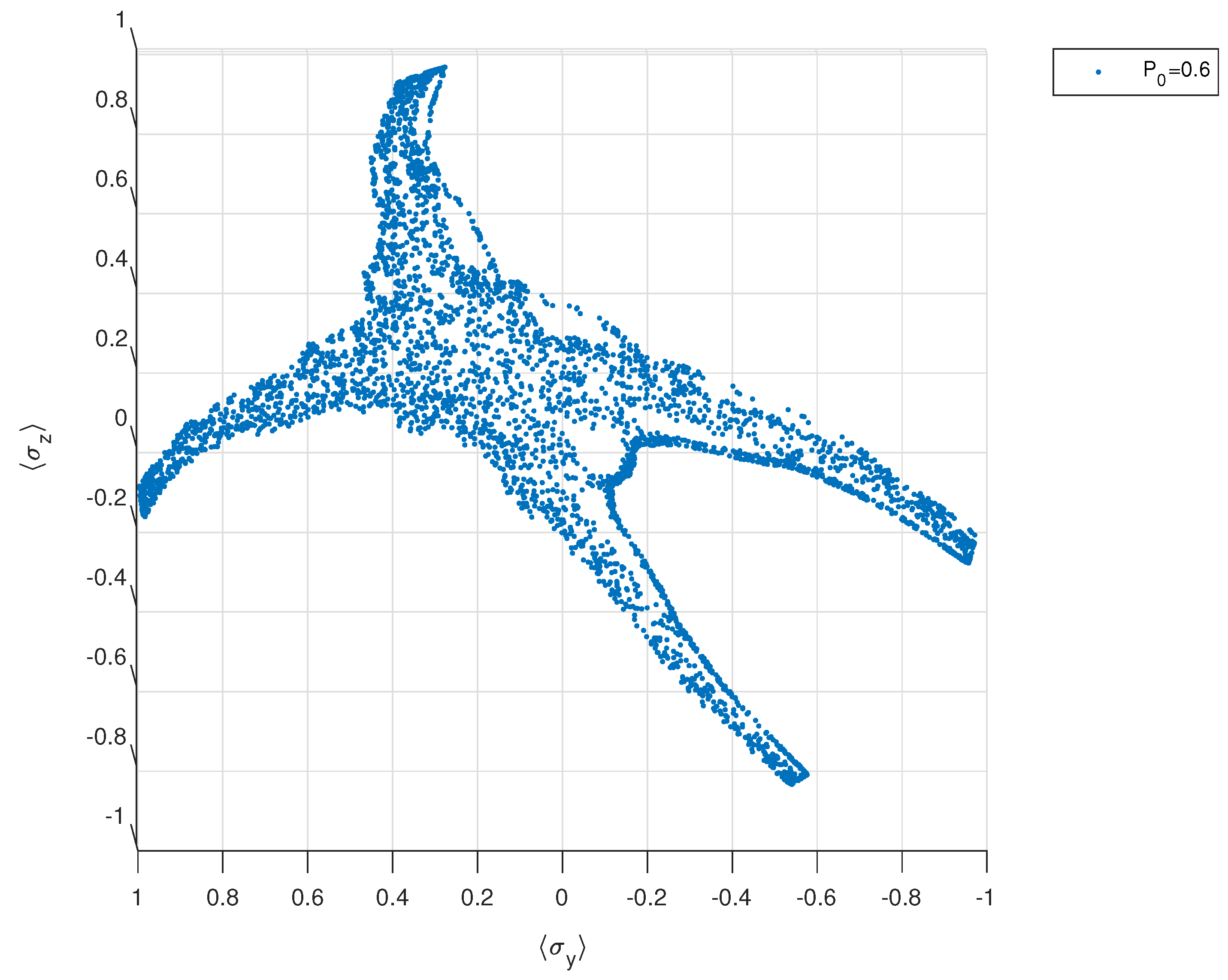
In Figure 4 and Figure 5, we show similar plots when the initial state has $P_0\left(0\right)=0.6$. Now the stroboscopic points are scattered over an irregular area and the spectrum is continuous. In Figure 6, the projection of the points on the Poincaré section $(\langle {\sigma }_x\rangle ,\langle {\sigma }_y\rangle )$ is shown. Thus, the initial wave function with $P_0\left(0\right)=0.6$ displays chaotic characteristics.

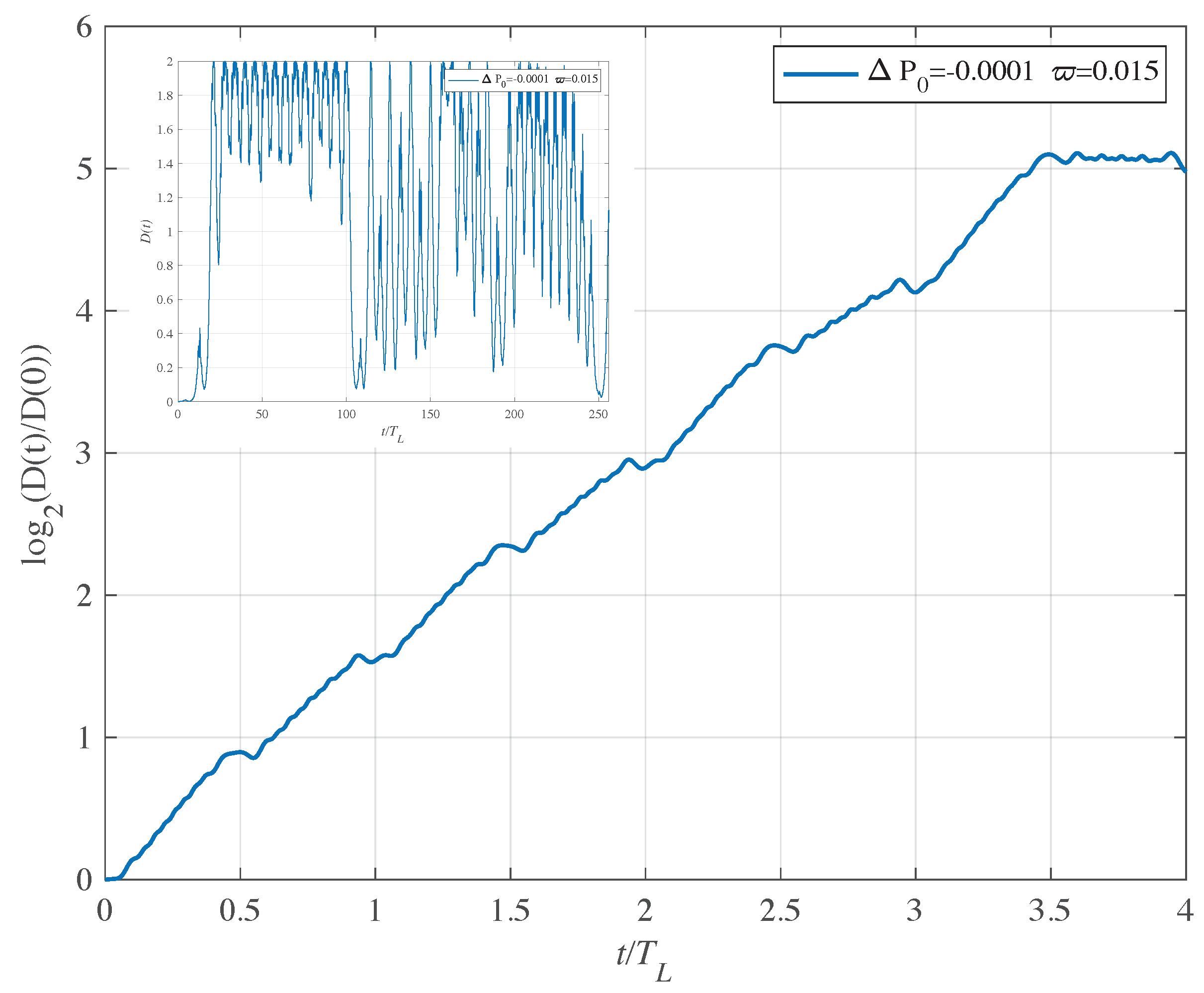
To prove that the behaviour is authentically chaotic we now evaluate the time evolution of the distance $D\left(t\right)=\sqrt{\Delta {\sigma }_1^2\left(t\right)+\Delta {\sigma }_2^2\left(t\right)+\Delta {\sigma }_3^2\left(t\right)}$ between two trajectories on the Bloch sphere with a nearby starting position. We note that the same procedure was adopted by Blümel and Esser [33]. In Figure 7 we show ${\log }_2\left(D\left(t\right)/D\left(0\right)\right)$ between the two orbits starting at $P_0\left(0\right)=0.6$ and $P_0\left(0\right)=0.6001$ versus time: we see that $D\left(t\right)$ is exponentially divergent with exponent $\lambda \cong 1.4$ oc${}^{-1}$. Before reaching the maximum distance $D=2$, $D\left(t\right)$ displays two more exponential growths with the same value of $\lambda$. In the inset, we show in linear scale $D\left(t\right)$: fast oscillations are clearly visible. A similar calculation, not shown here, performed for $P_0\left(0\right)=0$ where chaotic traits are not present does not present any exponential separation of the orbits. We conclude that the first Hamiltonian induces a chaotic evolution of the system.

2.2. Second Hamiltonian

An inspection of the form of the second Hamiltonian tells that the nonlinearity parameter ${\varpi }_2$ now plays a larger role than the one played by ${\varpi }_1$ in the first Hamiltonian. This happens because always $\varpi |c_0^{\ast }{c}_1|<\varpi$. Thus, chaotic behaviour should be found more easily in the second case. We shall see that the prediction is accomplished in a large measure. The value of the physical constants of the problem is unchanged with the exception of a smaller nonlinearity parameter, which now is ${\varpi }_2=1.0\times {10}^{-2}<{\varpi }_1=1.5\times {10}^{-2}$ au.

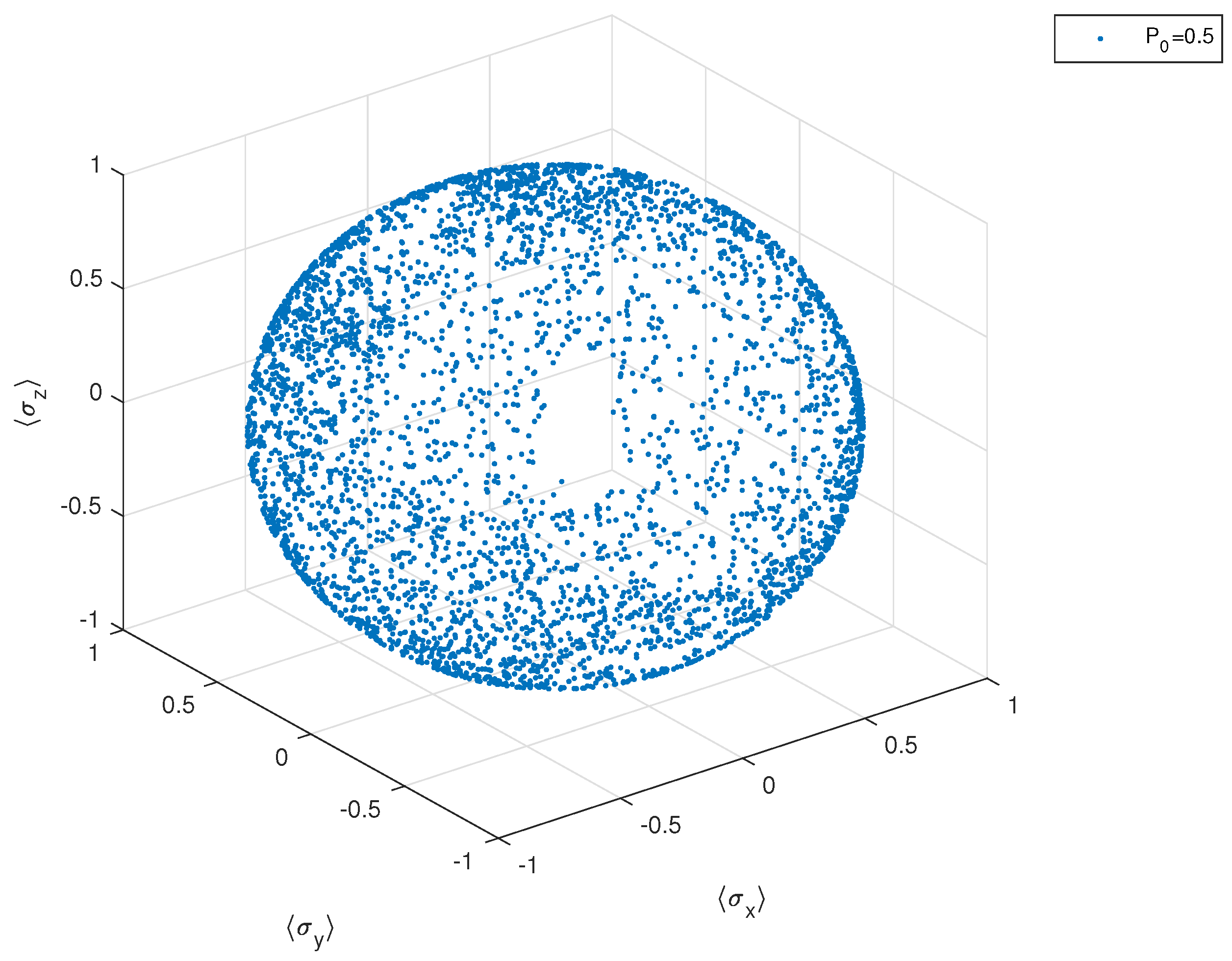
In Figure 8, we show the $\langle {\sigma }_i\rangle \left(n{T}_L\right)$ when the initial population of the ground state is $P_0=0.5$. The filling of the Bloch surface by the stroboscopic points seems uniform and no pattern can be recognized. This is a flag of chaos.

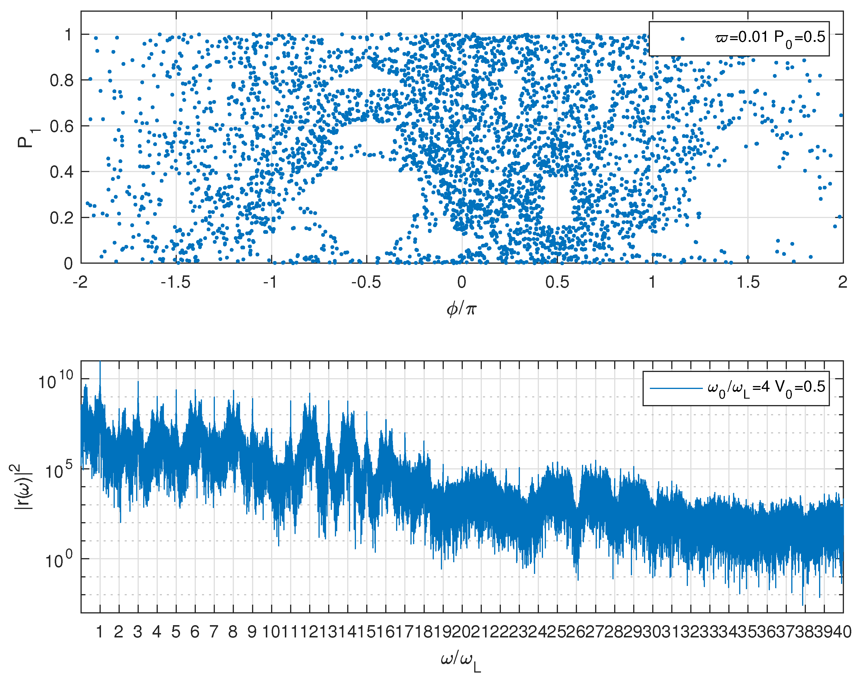
In Figure 9, we show $P_1\left(n{T}_L\right)$ vs. $\varphi \left(n{T}_L\right)/\pi$ and the power spectrum of the dipole moment when the initial population is $P_0=0.5$. The stroboscopic points are distributed in a random fashion and the power spectrum of the dipole moment is densely filled with unresolved lines. These features suggest that the evolution may be chaotic.

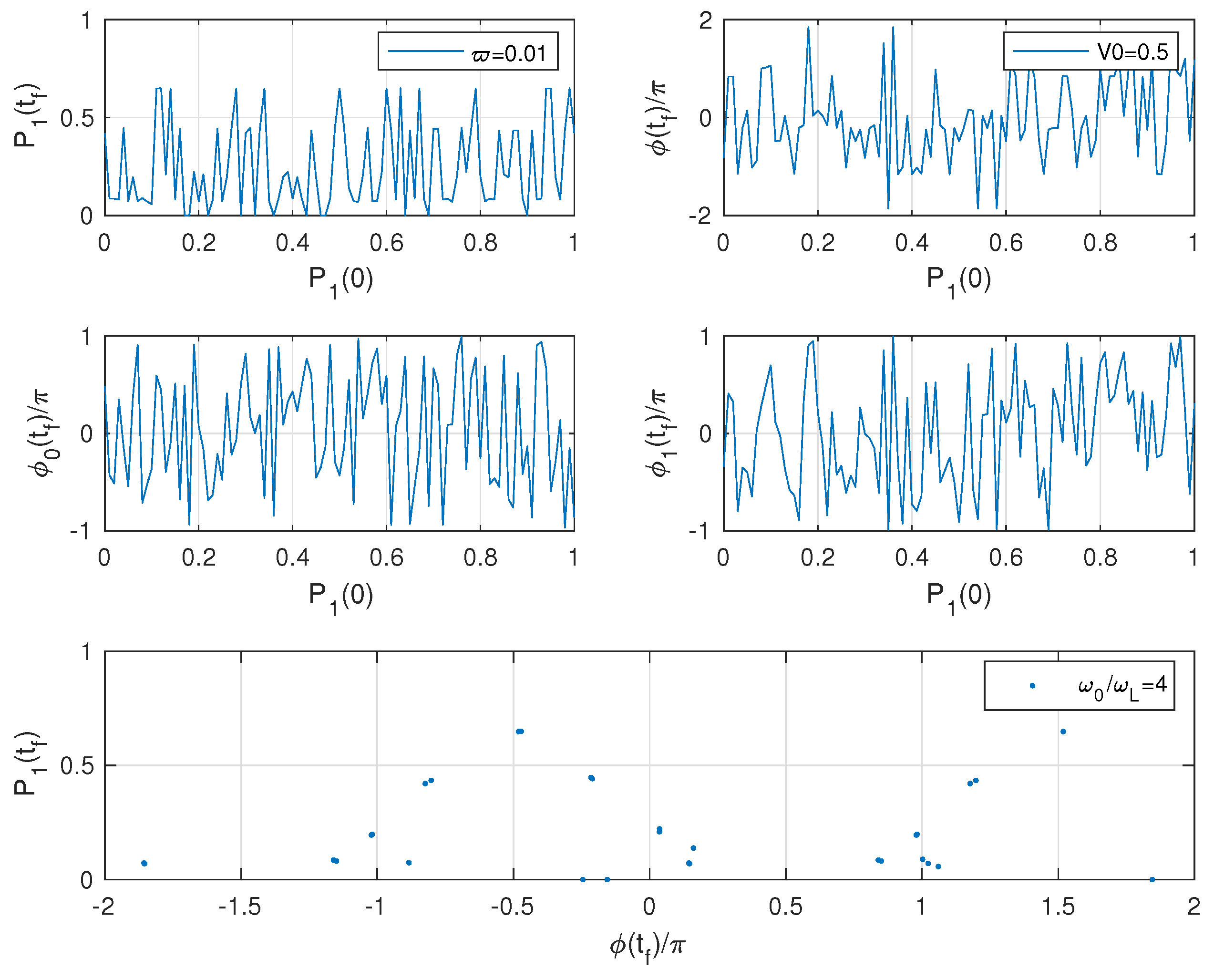
In Figure 10, we show the equivalent of Figure 1. The chaotic nature of the system is confirmed by the first two rows of plots. However, the last row is very surprising: the plot contains few stroboscopic points and not 100 as should be expected. Apparently the final phase difference and the final populations are correlated.

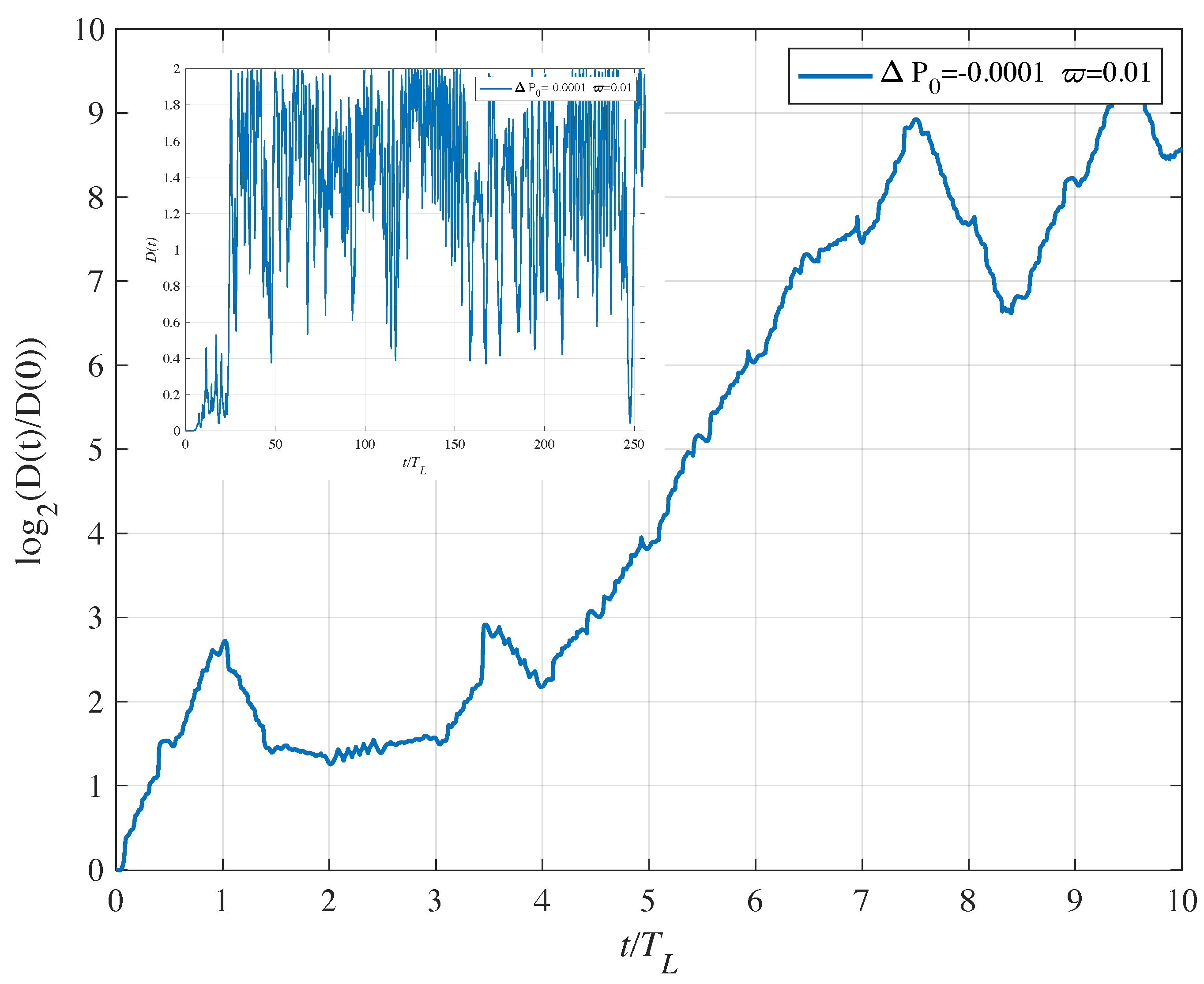
After these analyses, we resort again to the Lyapunov exponent to check that the second Hamiltonian introduces a bona fide chaotic evolution. In Figure 11, we show $D\left(t\right)$; we notice an exponential divergency in the time interval 4–7.5 oc where $\lambda \cong 1.9$ (oc)${}^{-1}$. In the full plot of $D\left(t\right)$, the maximum distance is reached after 20 oc and then fluctuates in a quick way not seen in the calculations for the first Hamiltonian. Again, we may say that the Lyapunov exponent confirms the qualitative conclusion that the motion is chaotic.

3. Final Remarks and Conclusions

In this paper we showed that the presence of a laser field may unveil and make detectable the presence of a small nonlinearity in the quantum Hamiltonian. We have argued that the nonlinearity may have different sources and the most probable one being extrinsic, caused by the need of modelling systems in which the dynamics are not fully known. In Classical Physics this is the main origin of nonlinearity; meteorology, fluid vortices, dissipative electric circuits, solar system and galaxy stability being the most common instances.

However, the possibility that a small intrinsic nonlinearity is present in the problem cannot be ignored. This second instance is a harbinger of many fundamental issues and is of deep debate. For example, the superposition principle is rudely put at stake as the superposition of two solutions of the nonlinear Schrödinger equation is not automatically a solution. Of course, also the essential technique of expanding the wave function as a linear combination of eigenstates is to be questioned and the use of a two-level atom used in the present calculations might lose validity and become a mere practical tool to be used because a fundamental theory is not available. However, qualitative information is important even more when a coherent theory is not known, at least in order to gain an idea on the phenomena to be looked at. We stress that it is legitimate to look for chaos in dealing with nonlinearity of extrinsic origin exactly in the same way as it has been done in Classical Physics.

Perhaps the connection between the nonlinear Schrödinger equation and the relativity principle represents the most important weakness for the research of intrinsic nonlinearity; in fact, almost from the beginning it has been realised that the presence of nonlinearity in Quantum Mechanics, at the least in the proposed forms, can be exploited for superluminal transmission of information [34,35,36,37]; thus an intrinsic nonlinear Schrödinger equation might be impossible. However, we believe that the nonlinear equations proposed up to now were meant with indicative meaning and that the relativity principle can be reconciled by a future fundamental theory of nonlinear Quantum Mechanics hopefully formulated in a relativistically covariant form. In this perspective, the finding of chaos in simple quantum systems may prove its importance. As yet much guessing work is required on the possible form of a quantum nonlinear Schrödinger equation; however, the actual form might be not really important because the emerging effect might be similar.

References

- Thompson, J.M.T.; Stewart, H.B. Nonlinear Dynamics and Chaos; John Wiley & Sons, LTD.: Hoboken, NJ, USA, 2002. [Google Scholar]
- Moon, F.C. Chaotic Vibrations an Introduction for Applied Scientists and Engineers; Wiley-Interscience: Hoboken, NJ, USA, 2004. [Google Scholar]
- Hilborn, R.C. Chaos and Nonlinear Dynamics; Oxford University Press: Oxford, UK, 1994. [Google Scholar]
- Vitiello, G. Classical Trajectories and Quantum Field Theory. Braz. J. Phys. 2005, 35, 351–358. [Google Scholar] [CrossRef]
- Davydov, A.S. Quantum Mechanics; International Series of Monographs in Natural Philosophy; Pergamon Press: London, UK, 1965; Volume I. [Google Scholar]
- Davydov, A.S. Solitons in molecular systems. Phys. Scr. 1979, 20, 387–394. [Google Scholar] [CrossRef]
- Kerr, W.C.; Lomdahl, P.S. Quantum-mechanical derivation of the equations of motion for Davydov solitons. Phys. Rev. B 1987, 35, 3629–3632. [Google Scholar] [CrossRef] [PubMed] [Green Version]
- Bayfield, J.E.; Koch, P.M. Multiphoton ionization of highly excited hydrogen atoms. Phys. Rev. Lett. 1974, 33, 258–261. [Google Scholar] [CrossRef]
- Bayfield, J.E.; Casati, G.; Guarneri, I.; Sokol, D.W. Localization of classically chaotic diffusion for hydrogen atoms in microwave fields. Phys. Rev. Lett. 1989, 63, 364–367. [Google Scholar] [CrossRef]
- Wyatt, R.E. Quantum Dynamics with Trajectories Introduction to Quantum Hydrodynamics; Interdisciplinary Applied Mathematics, 28; Springer: Berlin/Heidelberg, Germany, 2005. [Google Scholar]
- Efthymiopoulos, C.; Contopoulos, G. Chaos in bohmian quantum mechanics. J. Phys. A Math. Gen. 2006, 39, 1819–1852. [Google Scholar] [CrossRef]
- Dürr, D.; Teufel, S. Bohmian Mechanics: The Physics and Mathematics of Quantum Theory; Springer: Berlin/Heidelberg, Germany, 2009. [Google Scholar]
- Dürr, D.; Goldstein, S.; Zanghi, N. Quantum chaos, classical randomness, and bohmian mechanics. J. Stat. Phys. 1992, 68, 259–270. [Google Scholar] [CrossRef]
- De Polavieja, G.G. Exponential divergence of neighboring quantal trajectories. Phys. Rev. A 1996, 53, 2059–2061. [Google Scholar] [CrossRef]
- Bonfim, O.F.D.; Florencio, J.; Barreto, F.C.S. Chaotic dynamics in billiards using Bohm’s quantum mechanics. Phys. Rev. E 1998, 58, R2693–R2696. [Google Scholar] [CrossRef] [Green Version]
- De Alcantara Bonfim, O.F.; Florencio, J.; Sá Barreto, F.C. Quantum chaos in a double square well: An approach based on Bohm’s view of quantum mechanics. Phys. Rev. E 1998, 58, 6851–6854. [Google Scholar] [CrossRef] [Green Version]
- Ivanov, I.A.; Nam, C.H.; Kim, K.T. Quantum chaos in strong field ionization of hydrogen. J. Phys. B At. Mol. Opt. Phys. 2019, 53, 225002. [Google Scholar] [CrossRef]
- Weinberg, S. Precision tests of quantum mechanics. Phys. Rev. Lett. 1989, 62, 485–488. [Google Scholar] [CrossRef] [PubMed]
- Heinzen, D.J.; Bollinger, J.J.; Itano, W.M.; Gilbert, S.L.; Wineland, D.J. Test of the linearity of quantum mechanics by rf spectroscopy of the 9Be+ ground state. Phys. Rev. Lett. 1989, 63, 1031. [Google Scholar]
- Bialynicki-Birula, I. On the linearity of the Schrödinger equation. Braz. J. Phys. 2005, 35, 211–215. [Google Scholar] [CrossRef]
- Dou, G.-Q.; Cao, H.; Liu, J.; Fu, L.-B. High-fidelity composite adiabatic passage in nonlinear two-level systems. Phys. Rev. A 2016, 93, 043419. [Google Scholar] [CrossRef]
- Mittleman, M.H. Introduction to the Theory of Laser-Atom Interaction, 2nd ed.; Springer Science + Business Media, LLC: Berlin/Heidelberg, Germany, 1993. [Google Scholar]
- Joachain, C.J.; Kylstra, N.J.; Potvliege, R.M. Atoms in Intense Laser Fields; Cambridge University Press: Cambridge, UK, 2012. [Google Scholar]
- Cocke, S.; Reichl, L.E. High-harmonic generation in a driven triangular well: The implications of chaos. Phys. Rev. A 1996, 53, 1746–1750. [Google Scholar] [CrossRef]
- Corso, P.P.; Fiordilino, E.; Persico, F. Space-time localization of the radiation emitted by an electromagnetically driven charge and the question of the position of an electron. J. Mod. Opt. 2003, 50, 643–655. [Google Scholar] [CrossRef]
- Corso, P.P.; Fiordilino, E.; Persico, F. The electron wavefunction in laser-assisted bremsstrahlung. J. Phys. B At. Mol. Opt. Phys. 2003, 36, 2823–2835. [Google Scholar] [CrossRef]
- Xia, Y.; Jaron-Becker, A. Mollow sidebands in high order harmonic spectra of molecules. Opt. Express 2016, 24, 4689–4697. [Google Scholar] [CrossRef] [Green Version]
- Wolf, A.; Swift, J.B.; Swinney, H.L.; Vastano, J.A. Determining Lyapunov exponents from a time series. Physica 1985, 16D, 285–317. [Google Scholar] [CrossRef] [Green Version]
- Milonni, P.W.; Ackerhalt, J.R.; Galbraith, H.W. Chaos in the semiclassical n-atom Jaynes-Cummings model: Failure of the rotating-wave approximation. Phys. Rev. Lett. 1983, 50, 966–969. [Google Scholar] [CrossRef]
- Fiordilino, E. Chaos and nonlinearities in high harmonic generation. Laser Phys. Lett. 2016, 13, 115302. [Google Scholar] [CrossRef] [Green Version]
- Seiferle, B.; von der Wense, L.; Bilous, P.V.; Amersdorffer, I.; Lemell, C.; Libisch, F.; Stellmer, S.; Schumm, T.; Düullmann, C.E.; Pálffy, A.; et al. Energy of the 229Th nuclear clock transition. Nature 2019, 573, 243. [Google Scholar] [CrossRef] [PubMed] [Green Version]
- Huntemann, N.; Lipphardt, B.; Tamm, C.; Gerginov, V.; Weyers, S.; Peik, E. Improved limit on a temporal variation of mp/me from comparisons of Yb+ and Cs atomic clocks. Phys. Rev. Lett. 2014, 113, 210802. [Google Scholar] [CrossRef] [Green Version]
- Blümel, R.; Esser, B. Quantum chaos in the Born-Oppenheimer approximation. Phys. Rev. Lett. 1994, 72, 3658–3661. [Google Scholar] [CrossRef]
- Gisin, N. Weinberg’s non-linear quantum mechanics and supraluminal communications. Phys. Lett. A 1990, 143, 1–2. [Google Scholar] [CrossRef]
- Czachor, M. Mobility and non-separability. Found. Phys. Lett. 1991, 4, 351–361. [Google Scholar] [CrossRef]
- Polchinski, J. Weinberg’s nonlinear quantum mechanics and the Einstein-Podolsky-Rosen paradox. Phys. Rev. Lett. 1991, 66, 397–400. [Google Scholar] [CrossRef]
- Jordan, T.F. Why quantum dynamics is linear. J. Phys. Conf. Ser. 2009, 196, 012010. [Google Scholar] [CrossRef]
Figure 1.
First Hamiltonian. First row: final population of the upper level as a function of its initial population and relative phase between the two states vs. . Second row and vs. . Third row vs. . All plots contain 100 points.
Figure 2.
First Hamiltonian. First row: vs. where n is an integer and the laser period. Second row, spectrum emitted by the atom. The atom starts from the ground state.
Figure 3.
First Hamiltonian. The vector stroboscopically plotted at .
Figure 4.
First Hamiltonian. First row: vs. where n is an integer and the laser period. Second row, spectrum emitted by the atom. The initial population of the ground state is .
Figure 5.
Figure 6.
Figure 7.
First Hamiltonian. Plot of vs. of two orbits that start with close initial conditions. For the first orbit and for the second orbit . The value of the Lyapunov exponent is oc. In the inset, the time evolution of is shown in linear scale for the first oc.
Figure 8.
Second Hamiltonian. The vector stroboscopically plotted at .
Figure 9.
Second Hamiltonian. First row: vs. where n is an integer and the laser period. Second row, spectrum emitted by the atom. The initial population of the ground state is .
Figure 10.
Second Hamiltonian. First row: final population of the upper level as a function of the its initial population and relative phase between the two states vs. . Second row and vs. . Third row vs. . All plots contain 100 points.
Figure 11.
Second Hamiltonian. Plot of vs. of two orbits that start with close initial condition. For the first orbit and for the second orbit . The value of the Lyapunov exponent is oc. In the inset the full time evolution of is shown in linear scale.
© 2020 by the author. Licensee MDPI, Basel, Switzerland. This article is an open access article distributed under the terms and conditions of the Creative Commons Attribution (CC BY) license (http://creativecommons.org/licenses/by/4.0/).
Share and Cite
MDPI and ACS Style
Fiordilino, E. The Emergence of Chaos in Quantum Mechanics. Symmetry 2020, 12, 785. https://0-doi-org.brum.beds.ac.uk/10.3390/sym12050785
AMA Style
Fiordilino E. The Emergence of Chaos in Quantum Mechanics. Symmetry. 2020; 12(5):785. https://0-doi-org.brum.beds.ac.uk/10.3390/sym12050785
Chicago/Turabian StyleFiordilino, Emilio. 2020. "The Emergence of Chaos in Quantum Mechanics" Symmetry 12, no. 5: 785. https://0-doi-org.brum.beds.ac.uk/10.3390/sym12050785
Note that from the first issue of 2016, this journal uses article numbers instead of page numbers. See further details here.