Symmetries and Metamorphoses

Abstract

In quantum field theory with spontaneous breakdown of symmetry, the invariance of the dynamics under continuous symmetry transformations manifests itself in observable ordered patterns with different symmetry properties. Such a dynamical rearrangement of symmetry describes, in well definite formal terms, metamorphosis processes. The coherence of the correlations generating order and self-similar fractal patterns plays a crucial role. The metamorphosis phenomenon is generated by the loss of infrared contributions in physical states and observables due to their localized nature. The dissipative dynamics and evolution, the arising of the arrow of time and entanglement are also discussed. The conclusions may be extended to biology and neuroscience and to some aspects of linguistics in the transition from syntax to semantics (generation of meanings).

1. Introduction

The “change in form and structure” is often the protagonist in nature in all its aspects and the “question of metamorphosis” has always attracted much attention in the literature, arts and philosophy. In science the phenomenon of metamorphosis has been since a long time and is still today object of extended searches in the frame of evolutionistic theory and observations, in biology and botanic studies. The great land of fractal studies involving mathematics, statistical sciences and computer simulations offers on the other hand more and more occasions of explorations and applications to many sectors of engineering and science.

However, one less explored possibility in the study of the metamorphosis phenomenon is the one offered by the quantum field theory (QFT) of particle physics and condensed matter physics. Aim of this work is to show how the observable manifestations of dynamical symmetries in QFT may be described in well definite formal terms as metamorphoses. The metamorphosis phenomenon then appears in its genuine dynamical feature.

In the following, the discussion will rest on known QFT results, reviewed by resorting to specific general mechanisms, such as the spontaneous breakdown of symmetry (SBS) (Section 2 and Section 3), the group contraction mechanism in the dynamical rearrangement of symmetry (Section 4 and Section 5), the effects due to the system boundaries (Section 6). Fractal self-similarity properties and q-deformed coherent states, properties of functional stability, entanglement, dissipation, non-unitary time evolution (the arrow of time) are also briefly discussed (Section 7 and Section 8). Section 9 is devoted to the conclusions.

The localized character of physical states in finite space–time regions and the consequent loss of infrared contributions is found to be at the origin of the metamorphosis dynamical processes. The coherence of the condensate structure of the ground state (the vacuum structure) is responsible for the endless evolution [1] of forms along the flow of the arrow of time in morphogenesis processes.

The conclusions may be extended to gauge field theories and finite temperature systems. The discussion is limited to internal symmetries described by continuous compact symmetry groups. Nevertheless, we will also see that “external” (space and time) symmetries can be affected by the breakdown phenomenon. For example, the breakdown of time-reversal symmetry in open systems leads us also to the breakdown of time translational symmetry (and thus of Lorentz symmetry in a relativistic theory) (cf. Section 8). Breakdown of continuous space translational symmetry occurs, for example, in the case of crystals, where the symmetry rearrangement leads us to the crystal lattice structure. However, for brevity I only mention it in Section 5. Similarly, I will only spend a few words about the breakdown of time translation and time-reversal symmetry in connection with quantization in the curved background and inflation in cosmology (Section 8). Details of these and other issues are thus not discussed in the present work. The interested reader is referred to the quoted literature.

In order to facilitate the reading, mathematical details are summarized and partially confined in the appendices.

2. Two Levels of Description in Quantum Field Theory

In QFT there are representations of the canonical commutation relations (CCR for bosons; canonical anticommutation relations (CAR) for fermions) that cannot be related to each other by unitary transformations. In fact, infinitely many of them exist in QFT [2,3,4,5,6,7,8,9]. As is customary, I will refer to them as “unitarily inequivalent representations” (uir) of the CCR (CAR). In this section my comments are focused on such a specific feature of QFT, not present in quantum mechanics (QM), where the representations of the CCR (CAR) are unitarily equivalent [10]. The occurrence of uir in QFT is due to the fact that the number of degrees of freedom carried by fields is by definition an infinite number, which invalidates the proof of unitary equivalence holding instead in QM.

The mathematical issue of unitary equivalence or non-equivalence of the representations is of special physical relevance since it is actually the issue of physical equivalence or not of the corresponding dynamical regimes of the system under study. For example, the ferromagnetic and the non-ferromagnetic phases are described by uir and denote dynamical regimes with physical different properties of the same system of elementary constituents (similarly, the superconductive and non-superconductive phases, the crystal and the amorphous phases, etc.).

The conclusion is that the ‘same’ system (e.g., the same piece of material) may appear in the observations with physical properties that are mutually exclusive, in the example of ferromagnets with zero or non-zero magnetization M. Unitary inequivalence means that there is no unitary transformation able to change the value of the magnetization. The system actually is observed to be in one of the representations (Hilbert spaces) $H_F$ associated to one of the possible values of M, each representation being orthogonal to the other ones. This means that the ferromagnetic state of given magnetization M cannot be given by a superposition of states of magnetization $M^{\prime },M^{″},\dots$ etc. Transitions through the representations $H_{F,M}$, each one associated to a specific value of M, (phase transitions) are actually possible [11]. However, they are “singular” transitions, meaning that they involve some kind of “criticality”, thus not surprisingly involving the divergence of some quantity (e.g., susceptivity).

The dynamics of elementary constituents manifests itself in physical states and observables given in terms of physical fields $\varphi \left(x\right)$, $x\equiv \mathbf{x},t$, satisfying linear field equations

$$\Lambda (\partial )\varphi \left(x\right)=0$$

(1)

and having CCR (if boson fields) or canonical anticommutation relations (CAR) (if fermion fields). This is the physical level of description. $\Lambda (\partial )$ is a differential operator (projecting on the on-shell dispersion relation). Since $\varphi \left(x\right)$ are field operators, Equation (1) has to be understood as a ‘weak equality’, namely an equation for matrix elements computed in $H_F$, which means that we have to perform our choice of the state space $H_F$, on which we want to work, among the set $\left\{H_F\right\}$ of the infinitely many uir. In QM there is no need to do such a choice since the representations are unitary equivalent [10].

Consider now the other level of description, the dynamical level. QFT is assumed to be a canonical theory where the dynamics is specified by the Lagrangian L. The discussion is thus focused on closed systems described by canonical formalism. The basic entities describing the interaction are called Heisenberg fields. Denote them by $\psi \left(x\right)$. They satisfy the equations derived from L,

$$\Sigma (\partial )\psi \left(x\right)=F\left(\psi \right(x\left)\right),$$

(2)

and have CCR (CAR). $\Sigma (\partial )$ is a convenient operator describing kinematical terms and F is non-linear in the $\psi \left(x\right)$ fields. These are field operators defined on some Hilbert space $\mathcal{H}$. Equation (2), like Equation (1), is therefore meaningful only provided $\mathcal{H}$ is assigned (it is a weak equality). However, we do not have access to such a space. We have access only to physical states in $H_F$. Such a situation imposes to us to consider the mapping between $\psi \left(x\right)$ and $\varphi \left(x\right)$ fields (the dynamical map or the Haag expansion):

$$\psi \left(x\right)=\mathsf{\Psi }\left(\varphi \right(x\left)\right),$$

(3)

which again has to be understood as a weak equality in $H_F$. Matrix elements of $\psi \left(x\right)$ fields can be then computed in $H_F$.

I remark that the numbers of the $\psi$ and $\varphi$ fields need to be not necessarily the same. A bound state, for example, might be created out of a number of interacting $\psi$ fields. Another physical field is thus obtained. Physical fields must constitute anyway an irreducible set of fields.

Let me mention also that $\mathcal{H}$ and $H_F$ are unitarily inequivalent spaces (the Haag theorem) [2,3,4,8,12]. Apart from crucial consequences at the structural and computational level, such as the need of non-perturbative physics, the Haag theorem confirms that we have access to the dynamics of the basic $\psi \left(x\right)$ fields only through its manifestation in terms of physical fields $\varphi \left(x\right)$ and physical states. An intrinsic “opacity” of the basic dynamics is built-in in our knowledge [13].

It may happen that in one or more of the spaces $H_F$, the vacuum $|0\rangle$ is not symmetric under the symmetry group G of the Lagrangian, but only under one of its subgroup (called the stability group). One then says that the spontaneous breakdown of symmetry (SBS) occurs (in this work I am not interested in the “explicit” breakdown of symmetry obtained by introducing a symmetry breaking term in the Lagrangian).

Suppose we have SBS. Let $g\in G$ be an invariant transformation of the Heisenberg field $\psi \left(x\right)$

$$\psi \left(x\right)\to {\psi }^{\prime }\left(x\right)=g\left[\psi \left(x\right)\right].$$

(4)

Through the dynamical map (3) the transformation (4) can be obtained by the transformation $t\in G^{\prime }$ of the fields $\varphi$

$$\varphi \left(x\right)\to {\varphi }^{\prime }\left(x\right)=t\left[\varphi \left(x\right)\right],$$

(5)

giving

$$g\left[\psi \right(x\left)\right]=\mathsf{\Psi }\left(t\right[\varphi \left(x\right)\left]\right).$$

(6)

When $G^{\prime }\ne G$ we have the dynamical rearrangement of symmetry $G\to G^{\prime }$ [5,6,7,14,15,16,17,18,19].

As shown in the next section, SBS implies that observable ordered patterns, identified by an “order parameter”, are dynamically generated in $|0\rangle$. The specificity and the value of the order parameter depend on the considered, specific representation $H_F$.

Summing up, the same dynamics ruled by (2) may manifest itself in the infinitely many different realizations offered by the inequivalent physical representations $\left\{H_F\right\}$. One aspect of the success of QFT in describing a multitude of physical phenomena resides in such a tremendous richness.

Symmetry patterns in physical states are observable realizations of the invariance of the dynamics.

3. Spontaneous Breakdown of Symmetry

I will consider the ferromagnet as an example. Transformations of the continuous $SU\left(2\right)$ group are symmetry transformations for the Lagrangian and Heisenberg equations. The $ϵ$-term in the generating functional (see Appendix A) describes the coupling of the system with an external agent (the environment) and triggers the SBS (choice of $H_F$) [20]. The dynamics thus “realizes” itself in the broken symmetry state, where the system stays also in the absence of the environment action ($ϵ\to 0$) and is characterized by the magnetization M (the order parameter).

The magnetized (ground) state $|0\rangle$ is not symmetric under the three parameters $SU\left(2\right)$ group (three axis spherical rotations), but only under rotations around the magnetization direction, e.g., the 3rd axis in the spin-space ($U\left(1\right)$ subgroup of $SU\left(2\right)$). However, the invariance of the theory is not “lost” at the level of physical fields since their equations are still invariant, as we will see, under a three-parameter group, the $E\left(2\right)$ group, although the basic symmetry is broken in $|0\rangle$. The conservation laws associated with the three $SU\left(2\right)$ generators commuting with the Hamiltonian cannot be lost since this would introduce a radical modification of the dynamics of our model (of its defining Lagrangian and Hamiltonian). What happens is that the invariance, defined by such vanishing commutators, unfolds itself in different symmetry patterns, it manifests itself under different physical “appearances”. A metamorphosis process, indeed.

Changes in the order parameter correspond to transitions among the “phases” $H_F$’s (phase transitions). Our conclusions, although derived for the ferromagnets, hold in their structural aspects for any system whose Lagrangian is symmetric under continuous compact symmetry group transformations.

In the itinerant electron model of ferromagnets the Heisenberg electron field is

$$\psi \left(x\right)=\left(\begin{array}{c}{\psi }_{\uparrow }\left(x\right)\hfill \\ {\psi }_{\downarrow }\left(x\right)\hfill \end{array}\right),$$

(7)

where spin up and spin down are denoted by ↑ and ↓, respectively. They have usual equal-time CAR and the $SU\left(2\right)$ transformation is

$$\psi \left(x\right)\to {\psi }^{\prime }\left(x\right)=exp\left(i{\theta }_i{\lambda }_i\right)\psi \left(x\right),i=1,2,3,$$

(8)

${\sigma }_i$ are the Pauli matrices, ${\lambda }_i={\sigma }_i/2$, the rotation angles in the spin-space ${\theta }_i$ are real and denote the continuous group parameters. The explicit expression of the Lagrangian is not needed here; it is only required to be symmetric under the $SU\left(2\right)$ transformations (8), i.e., $\mathcal{L}\left[\psi \left(x\right)\right]=\mathcal{L}\left[{\psi }^{\prime }\left(x\right)\right]$. The explicit expression of the $SU\left(2\right)$ spin density $S_{\psi }^{\left(i\right)}\left(x\right),i=1,2,3$, does not need to be specified (one possible form is $S_{\psi }^{\left(i\right)}\left(x\right)={\psi }^{†}\left(x\right)\left({\sigma }_i/2\right)\psi \left(x\right)$). The $SU\left(2\right)$ algebra is

$$[S_{\psi }^{\left(i\right)}\left(x\right),S_{\psi }^{\left(j\right)}\left(x\right)]=i{ϵ}_{ijk}{S}_{\psi }^{\left(k\right)}\left(x\right).$$

(9)

The essential steps in the functional integration formalism are presented in the Appendix A.

Let ${\mu }_B$ denote the Bohr magneton. $g{\mu }_B{\langle S_{\psi }^{\left(3\right)}\left(x\right)\rangle }_{ϵ}$ gives the magnetization. ${\langle S_{\psi }^{\left(3\right)}\left(x\right)\rangle }_{ϵ}$ is given in Equations (A7) and (A8) and represents the expectation value of the spin density in the third direction (the order parameter). $ϵ$ carries the information of the SBS. At the end of the computation we take the limit $ϵ\to 0$. Putting $M\left(ϵ\right)={\langle S_{\psi }^{\left(3\right)}\left(x\right)\rangle }_{ϵ}$ and

$$M=\underset{ϵ\to 0}{lim}M\left(ϵ\right),$$

(10)

$${\Delta }_i(ϵ,p)={\rho }_{\left(i\right)}\left(p\right)\left(\frac{1}{p_0-{\omega }_p+iϵa_i}-\frac{1}{p_0+{\omega }_p-iϵa_i}\right),$$

(11)

Equations (A7) and (A8) give

$$M\left(ϵ\right)=iϵ{\Delta }_i(ϵ,0),i=1,2,$$

(12)

showing that SBS, i.e., non-zero M, with $ϵ\to 0$ is possible only provided that ${\omega }_p=0$ at $p=0$. We then have $M=2\rho$ (cf. Appendix A).

The conclusion is therefore that the order parameter M can be different from zero provided that a bound state of gapless energy ${\omega }_p=0$ at $p=0$ exists. We have thus proved the Goldstone theorem in SBS theories [21], stating that SBS implies the existence of massless (gapless) modes or particles, the so called Nambu–Goldstone (NG) boson particles.

Summing up, the model independent proof has been given of the existence of the magnons (NG boson particles) in the $SU\left(2\right)$ SBS. Magnons are gapless (vanishingly small mass m) bound states of electrons, quanta of spin waves which by propagating over large distances R create long-range correlations among the spin components and thus ferromagnetic ordered patterns ($R\propto (1/m)\to \infty$).

4. Dynamical Rearrangement of Symmetry

I discuss now the rearrangement of $G\equiv SU\left(2\right)$ into $G^{\prime }$, the symmetry group of the equations of the quasielectron field $\varphi \left(x\right)$ (in solid state physics physical fields in the material are called quasiparticles) and the magnon boson field $\chi \left(x\right)$:

$$\Lambda \left(\overrightarrow{\partial }\right)\varphi \left(x\right)=0,K\left(\overrightarrow{\partial }\right){\chi }^{†}\left(x\right)=0.$$

(13)

$\varphi \left(x\right)$ and $\chi \left(x\right)$ form an irreducible set of fields. The electromagnetic field does not influence the main features of the rearrangement $G\to G^{\prime }$. Thus I do not consider it here (see below and [5] for further details). The $\chi \left(x\right)$ field commutation relations are

$${[\chi \left(x\right),{\chi }^{†}\left(y\right)]}_{t_x-t_y}=\delta (\mathbf{x}-\mathbf{y}).$$

(14)

Other commutators are zero and the dynamical map is

$$\psi \left(x\right)=\mathsf{\Psi }\left(\varphi \right(x),\chi (x\left)\right).$$

(15)

The S-matrix $\mathcal{S}$ and the spin densities $S^{\left(i\right)}\left(x\right)$ are obtained by using the Lehmann-Symanzik- Zimmerman (LSZ) formula

$$\mathcal{S}(\varphi ,{\varphi }^{†},\chi ,{\chi }^{†})=\langle :exp[-iA(\varphi ,{\varphi }^{†},\chi ,{\chi }^{†})]:\rangle$$

(16)

$$S^{\left(i\right)}(\varphi ,{\varphi }^{†},\chi ,{\chi }^{†})=\langle S_{\psi }^{\left(i\right)}\left(x\right):exp[-iA(\varphi ,{\varphi }^{†},\chi ,{\chi }^{†})]:\rangle ,i=1,2,3,$$

(17)

where $A(\varphi ,{\varphi }^{†},\chi ,{\chi }^{†})$ is given in the Appendix B. Normal ordering and functional average are denoted by $:\dots :$ and $\langle \dots \rangle$, respectively.

The transformed fields are denoted by ${\varphi }_{\theta },{\varphi }_{\theta }^{†},{\chi }_{\theta },{\chi }_{\theta }^{†}$ and the transformations are found to be (cf. Appendix B)

$$\begin{array}{ccc}\hfill \varphi \left(x\right)\to {\varphi }_{\theta }\left(x\right)& =& \varphi \left(x\right),\hfill \\ \hfill \chi \left(x\right)\to {\chi }_{\theta }\left(x\right)=\chi \left(x\right)& +& i{\theta }_1{\left(\frac{M}{2}\right)}^{\frac{1}{2}},\hfill \end{array}$$

(18)

for ${\theta }_2={\theta }_3=0$,

$$\begin{array}{ccc}\hfill \varphi \left(x\right)\to {\varphi }_{\theta }\left(x\right)& =& \varphi \left(x\right),\hfill \\ \hfill \chi \left(x\right)\to {\chi }_{\theta }\left(x\right)=\chi \left(x\right)& -& {\theta }_2{\left(\frac{M}{2}\right)}^{\frac{1}{2}},\hfill \end{array}$$

(19)

for ${\theta }_1={\theta }_3=0$, and

$$\varphi \left(x\right)\to {\varphi }_{\theta }\left(x\right)=e^{i{\theta }_3{\lambda }_3}\varphi \left(x\right),$$

$$\chi \left(x\right)\to {\chi }_{\theta }\left(x\right)=e^{-i{\theta }_3}\chi \left(x\right),$$

(20)

for ${\theta }_1={\theta }_2=0$ and their hermitian conjugates. Equations (18)–(20) are canonical transformations. Equation (20) is the (unbroken) $U\left(1\right)$ third axis rotation.

In conclusion, the $SU\left(2\right)$ symmetry is dynamically rearranged as shown by Equations (18)–(20) (to be compared to (8)). These are $E\left(2\right)$ group transformations, the Inönü–Wigner $SU\left(2\right)$ group contraction [19,22,23,24]. It is indeed a general result, confirmed in many examples in high energy and condensed matter physics, that in the presence of SBS, under quite wide conditions, the dynamical rearrangement $G\to G^{\prime }$ is controlled by the mathematical structure of group contraction [19,25,26]. A true metamorphosis process. We do not observe the symmetry of the dynamics but its physical manifestations.

The $SU\left(2\right)$ symmetry is “restored” as the temperature T raises above the critical temperature $T_C$ (the Curie temperature). However, provided $T<T_C$, the “forms” or “phases” we observe are the ferromagnetic ones. Moreover, changes in the magnetization (i.e., in the ‘forms’ of ordered patterns) are observed as T changes.

5. Homogeneous and Non-Homogeneous Boson Condensation

Since in SBS theories the ground state $|0\rangle$ is not symmetric under G, there must be at least one of the generators, say

$$D_n=\int d^{3}x{j}_0^{\left(n\right)}\left(x\right),$$

(21)

that does not annihilate $|0\rangle$, $D_n|0\rangle \ne 0$. The integration in Equation (21) extends over the (infinite) volume V and $j_0^{\left(n\right)}\left(x\right)$ is the zero component of the conserved current $j_{\mu }^{\left(n\right)}\left(x\right)$, ${\partial }_{\mu }{j}_{\mu }^{\left(n\right)}\left(x\right)=0$. The problem is to find the expression of the generators in terms of the physical fields (their dynamical maps). One can show that $D_n|0\rangle \ne 0$ is possible only provided that $D_n$ is linear in field operators [7,14,15].

Translational invariance of the vacuum implies that

$$\langle 0|D_n{D}_n|0\rangle =\int d^{3}x\langle 0|j_0^{\left(n\right)}\left(x\right)D_n|0\rangle$$

(22)

is a divergent quantity, which means that $D_n$ is mathematically not well defined, or, stated differently, the $D_n$ transformation is not unitarily implementable [3,5,12]. The state $e^{i\theta D_n}|0\rangle$ thus belongs to a representation which is unitarily inequivalent to the one to which $|0\rangle$ belongs, $\langle 0\left|e^{i\theta D_n}\right|0\rangle =0$ at $V\to \infty$.

The generator $D_n$ needs to be regularized to be mathematically well defined. This is done by writing

$$D_n\equiv \underset{f\left(x\right)\to 1}{lim}{D}_{f,n}=\underset{f\left(x\right)\to 1}{lim}\int d^{3}xf\left(x\right)j_0^{\left(n\right)}\left(x\right).$$

(23)

$f\left(x\right)$ is a square integrable function. We require that it is also solution of the equations for the fields appearing linearly in $j_0^{\left(n\right)}\left(x\right)$. This last constraint ensures that $D_{f,n}$ is time independent, as it needs to be since it is a symmetry generator (and the invariance of the dynamics is not violated at physical level). The regularization (23) amounts to take finite volume integration and the limit $V\to \infty$ (i.e., $f\left(x\right)\to 1$) at the end of computation.

The translations in (17) and (18) are thus the limit for $f\left(x\right)\to 1$ of $\chi \left(x\right)\to {\chi }_{\theta }\left(x\right)={lim}_{f\left(x\right)\to 1}(\chi \left(x\right)+f\left(x\right)c_j)$, with $c_j=i^j{\theta }_j{\left(M/2\right)}^{1/2},j=1,2$, and h.c.. $f\left(x\right)$ is a regular function, solution of the magnon equations, which are thus invariant under $\chi \left(x\right)\to \chi \left(x\right)+f\left(x\right)c_j$. The generators of (18)–(20) (with $f\left(x\right){\theta }_i$ replacing ${\theta }_i$) are

$$\begin{array}{ccc}\hfill s_f^{\left(1\right)}& =& {\left(\frac{M}{2}\right)}^{1/2}\int d^{3}x[\chi \left(x\right)f\left(x\right)+{\chi }^{†}\left(x\right)f^{*}\left(x\right)],\hfill \end{array}$$

(24)

$$\begin{array}{ccc}\hfill s_f^{\left(2\right)}& =& -i{\left(\frac{M}{2}\right)}^{1/2}\int d^{3}x[\chi \left(x\right)f\left(x\right)-{\chi }^{†}\left(x\right)f^{*}\left(x\right)],\hfill \end{array}$$

(25)

$$\begin{array}{ccc}\hfill s_f^{\left(3\right)}& =& \int d^{3}x[{\varphi }^{†}\left(x\right){\lambda }_3\varphi \left(x\right)-{\chi }^{†}\left(x\right)\chi \left(x\right)].\hfill \end{array}$$

(26)

Their commutation relations are:

$$\begin{array}{c}\hfill [s_f^{\left(1\right)},s_f^{\left(2\right)}]=iM\int d^{3}x{\left|f\left(x\right)\right|}^2=(const.)\mathbf{1},\end{array}$$

(27)

$$[s_f^{\left(3\right)},s_f^{\left(i\right)}]=i{ϵ}_{3ij}{s}_f^{\left(j\right)},$$

which is the (projective) $e\left(2\right)$ algebra. The introduction of the functions $f\left(x\right)$ is also understood by recalling that we consider weak equalities among physical states. These are observable states, and therefore smeared out, localized states. Thus they are naturally expressed in terms of square integrable functions, which are characterized by finite support (in space and time), going to zero at plus and minus infinity. Computing expectation values in physical states thus naturally introduces the use of square integrable functions.

Note that Equations (24) and (25) (or $s_f^{(\pm )}=(1/2)(s_f^{\left(1\right)}\pm i{s}_f^{\left(2\right)})$) are generators of coherent states [27,28]. The ferromagnet ground state is thus a coherent state of magnons. Coherent behaviors of microscopic components appear in the ordered patterns as manifestations of SBS, the “forms” in which the dynamics is realized, its metamorphosis.

Coherence is thus dynamically generated and through it the quantum dynamics manifest at the macroscopic level. In coherent states of coherent strength $\left|\alpha \right|$, the ratio of the fluctuations $\Delta n$ over the number n of condensed modes goes to zero for high $\left|\alpha \right|$ as $1/\left|\alpha \right|$, which leads to the classical behavior of the system [19,20]. Some of its properties can be derived only from the dynamics of its elementary components. The system is then defined to be a macroscopic quantum system. The order parameter, characterizing the system behavior, is indeed a classical quantity, not affected by quantum fluctuations (of course, except during phase transitions; moreover, under boundary conditions of strong coupling the semiclassical limit cannot be achieved, as discussed in [29]). In Section 8, also fractal self-similarity is shown to be isomorph to coherent state structure.

The dynamical rearrangements of symmetry, i.e., the metamorphosis process, thus signals the transition from the collection of individual components to their collective systemic coherent behavior. This is a general result. In the presence of the electromagnetic field, NG quanta do not belong to the set of observable particles. However, they still control the condensate of the vacuum. For brevity, here I do not discuss such a mechanism (see [5,30,31,32]).

In the limit $f\left(x\right)\to 1$ the boson condensation is space-time independent (homogeneous). However, without taking the $f\left(x\right)\to 1$ limit, it is also possible to consider non-homogeneous boson condensation. Homogeneous and non-homogeneous boson condensations are thus possible realizations of the invariance of the same dynamics (the boson transformation theorem [5,6]). The function $f\left(x\right)$, solution of physical field equations, may be Fourier integrable (regular function), or be divergent, or with topological singularities (singular function) generating the formation of extended objects with topological non-trivial singularities, such as vortices, solitons, monopoles, etc. [5,6,8,32,33]. $f\left(x\right)$ plays in such cases the role of a “form factor”.

Of particular interest is for example the case of crystal lattice structure since it involves the spontaneous breakdown of an “external” symmetry (continuous space translations). The lattice structure (space “discreteness”) is the result of the dynamical rearrangement of the continuous space translational symmetry [5]. The crystal periodic potential and related Bloch periodic functions are described by the q-deformation of Weyl-Heisenberg algebra [34,35].

Boson condensation with singularities is possible only for gapless bosons, as indeed is the case of NG bosons in SBS. This explains why the formation of objects with topological singularities is observed to occur in the presence of ordered patterns and in the phase transition processes. A rich diversity of forms is thus obtained, genuine morphogenesis processes.

6. The Origin of Metamorphoses

Physical states and observables are always localized in space and time. Therefore, so-called infrared terms, of the order of $1/V$, do not contribute to them. Let me analyze how the missing of infrared terms is at the origin of the metamorphosis process (the change of the symmetry algebra).

The magnon boson field $\chi \left(x\right)$ is given by

$$\chi \left(x\right)=\int \frac{d^{3}p}{{\left(2\pi \right)}^{3/2}}{\chi }_{\mathbf{p}}{e}^{i\mathbf{p}·\mathbf{x}-i{\omega }_{p}t},$$

(28)

with ${\omega }_p=0$ at $p=0$ (cf. Equation (12)). We can split $\chi \left(x\right)$ into ${\chi }_t\left(x\right)$, the “hard” part containing momenta larger than $\eta$, and ${\chi }_{\eta }\left(x\right)$, the “soft” or infrared part containing momenta smaller than $\eta$,

$$\chi \left(x\right)={\chi }_t\left(x\right)+{\chi }_{\eta }\left(x\right).$$

(29)

Note that ${\chi }_{\eta }\left(x\right)\propto \eta$ and it does not depend on x for $\eta \to 0$ (cf. Appendix C).

By using of (29) in (17) the contributions to the generators due to ${\chi }_{\eta }\left(x\right)$ can be identified. In the Appendix C it is shown that:

$$\begin{array}{ccc}\hfill S_f^{\left(1\right)}& =& s_f^{\left(1\right)}+{\left(\frac{1}{2M}\right)}^{1/2}({\chi }_{\eta }+{\chi }_{\eta }^{†}):s_t^{\left(3\right)}:,\hfill \end{array}$$

(30)

$$\begin{array}{ccc}\hfill S_f^{\left(2\right)}& =& s_f^{\left(2\right)}-i{\left(\frac{1}{2M}\right)}^{1/2}({\chi }_{\eta }-{\chi }_{\eta }^{†}):s_t^{\left(3\right)}:,\hfill \end{array}$$

(31)

$$\begin{array}{ccc}\hfill S_f^{\left(3\right)}& =& s_t^{\left(3\right)}+{\left(\frac{1}{2M}\right)}^{1/2}\left[i({\chi }_{\eta }-{\chi }_{\eta }^{†})s_t^{\left(2\right)}-({\chi }_{\eta }+{\chi }_{\eta }^{†})s_t^{\left(1\right)}\right].\hfill \end{array}$$

(32)

The $su\left(2\right)$ algebra is then recovered by computing

$$\underset{\eta \to 0}{lim}\underset{\overline{\eta }\to 0}{lim}\underset{f\to 1}{lim}[S_f^{\left(i\right)},S_f^{\left(j\right)}]=i{ϵ}_{ijk}{S}^{\left(k\right)},$$

(33)

where $\eta$ and $\overline{\eta }$ are used for the two rotations in the commutator. Thus

$$[S_f^{\left(i\right)},S_f^{\left(j\right)}]=i{ϵ}_{ijk}{S}^{\left(k\right)}.$$

(34)

Instead, the $e\left(2\right)$ algebra is obtained if the infrared contributions are missed:

$$\begin{array}{ccc}\hfill \underset{f\to 1}{lim}\underset{\tilde{\eta }\to 0}{lim}[S_f^{\left(1\right)},S_f^{\left(2\right)}]& =& iM\underset{f\to 1}{lim}\int d^{3}x{\left|f\left(x\right)\right|}^2=\left(const\right)\mathbf{1},\hfill \end{array}$$

(35)

$$\begin{array}{ccc}\hfill \underset{f\to 1}{lim}\underset{\tilde{\eta }\to 0}{lim}[S_f^{\left(3\right)},S_f^{\left(i\right)}]& =& \underset{f\to 1}{lim}\underset{\tilde{\eta }\to 0}{lim}i{ϵ}_{3ij}{S}^{\left(j\right)},\hfill \end{array}$$

(36)

with $\tilde{\eta }$ denoting the $\mathrm{minimum}\mathrm{of}\eta \mathrm{and}\overline{\eta }$.

Thus we have two non commuting limits, $f\to 1$ and $\overline{\eta }\to 0$. The commutators of the generators expressed in terms of physical fields are not affected by infrared terms (the group contraction algebra $e\left(2\right)$). Instead, these terms globally contribute to the $S^{\left(i\right)}$ commutators expressed in terms of the Heisenberg field (recovered by including the whole volume in the $f\to 1$ limit and adding up all the infrared contributions). In conclusion, the metamorphosis $SU\left(2\right)\to E\left(2\right)$ finds its root in the localized nature of physical states and observables.

I remark that the result presented here is fully general and exact, not derived in a linear approximation (as for example in the Holstein–Primakoff representation [36]).

Finally, I remark that the localization of physical states and observables is also a prerequisite for the locality and causality principle. When we say that QFT is a local theory, we mean that a system A may be influenced by another system B, which is at some distance $\delta$ from A, through the exchange of a quantum traveling at a speed not higher than the light speed c. This is required by relativity and guaranties that the causality principle is also satisfied (the effect necessarily follows in time the cause (at a $\Delta t\ge \delta /c$)). The basic requirement for the locality is of course that A is distinguishable from B, i.e., they are localized in finite, separate space-time regions.

Let me estimate in a concrete example the order of magnitude of the localization of a low energy electron. Consider e.g., a thermal electron moving in the z direction with kinetic energy $E_{k_z}\approx (1/40)$ eV. $\mathbf{k}$ is the wave vector. For simplicity, the plane wave approximation is used. Let $\Delta x<<L$, with L the linear size of the instrument surface detecting the electron, say of the order of millimeters. The motion direction is well-defined if the transverse component of the wave vector is small compared to $k_z$, thus assume $\Delta k_x/k_z<<1$ (we will see that assuming this of the order of ${10}^{-5}$ will fit the instrument constraint). Due to the Heisenberg uncertainty relation, it is $1/(k_z\Delta x)\le (\Delta k_x/k_z)$. From $E_{k_z}={\hslash }^2{k}_z^2/2m$ (with $p_z=\hslash k_z$) it is derived $1/k_z=(\hslash /mc){(m{c}^2/2E_{k_z})}^{1/2}$. Use of $m{c}^2=0,5\times {10}^6$ eV and $\hslash /mc=3,861\times {10}^{-11}$ cm (the Compton wave length of the electron) gives $1/k_z={10}^{-7}$ cm. Using this value in $1/(k_z\Delta x)\le {10}^{-5}$ gives $\Delta x\ge {10}^{-2}$ cm, which can easily satisfy the instrument condition $\Delta x<<L$. Note that the obtained result justifies the use of the wave plane approximation (instead of the electron wave packet description) (further details in [37]).

7. Boundary Effects in Spontaneous Breakdown of Symmetry

In Equation (A10) the integration over the infinite volume selects the zero-momentum in the two-point correlation function. The system volume finiteness, however, produce effects on the system order, e.g., distortions of symmetry patterns due to boundary effects. On the other hand, the system boundaries by themselves might be dynamically created, not imposed by some external agent. The boundaries and the size of symmetry patterns in non-homogeneous condensation are in fact dynamically generated. Processes of fragmentation of ordered domains into smaller domains might be indeed described by the reduction of the extension of the ordering correlation range.

Consider Equations (A7), (A8) and (A10). Restrict the integration to finite volume $V\equiv {\eta }^{-3}$. Since

$${\delta }_{\eta }\left(p\right)=\frac{1}{2\pi }{\int }_{-\frac{1}{\eta }}^{\frac{1}{\eta }}dx{e}^{ipx}=\frac{1}{\pi p}sin\frac{p}{\eta },$$

(37)

and ${lim}_{\eta \to 0}{\delta }_{\eta }\left(p\right)=\delta \left(p\right)$ we have

$$\underset{\eta \to 0}{lim}\int dp{\delta }_{\eta }\left(p\right)f\left(p\right)=f\left(0\right)=\underset{\eta \to 0}{lim}\int dp\delta (p-\eta )f\left(p\right).$$

(38)

Since ${\delta }_{\eta }\left(p\right)\simeq \delta (p-\eta )$ for small $\eta$, we get (cf. Equation (11))

$$M(ϵ,\eta ,\mathbf{y})=iϵe^{-i\eta ·\overrightarrow{y}}{\Delta }_i(ϵ,\eta ,p_0=0),i=1,2,$$

(39)

Thus, provided ${\omega }_{\overrightarrow{p}=\eta }=0$ for $\eta \to 0$, ${lim}_{ϵ\to 0}{lim}_{\eta \to 0}M(ϵ,\eta ,\mathbf{y})\ne 0$. We see that for $\eta \to 0$ (infinite volume limit) the Goldstone theorem holds. However, it is ${lim}_{ϵ\to 0}M(ϵ,\eta ,\mathbf{y})=0$ for non-zero $\eta$ (finite volume, boundary effect); the $\chi$ bosons behave as having an “effective mass” $\propto {\omega }_{\overrightarrow{p}=\eta }\ne 0$. Then, $M\ne 0$ only if $ϵ\ne 0$. $ϵ$ plays the role of the pump supplying energy.

Our conclusions, although derived for the case of ferromagnets, are fully general [20]. In the presence of boundaries an effective mass $m_{eff}$ is generated for the correlation quanta and the condensation domain has linear size $\propto \xi \equiv 1/m_{eff}$. In general, “distorsions” of the condensate may occur “near” the boundaries. Conversely, if NGs acquire an effective mass due to action of some external agent (e.g., thermal effects), then the system dynamically rearranges so that condensation regions of size $\propto 1/m_{eff}$ are formed [38] within boundaries dynamically generated (fragmentation of ordered patterns), or else “symmetry restoration” (transition to disordered phase) may occur for $\xi \to 0$.

Symmetry restoration typically occurs due to thermalization when temperature T becomes larger than the critical temperature $T_C$. Then, $m_{eff}\propto \sqrt{\frac{|T-T_C|}{T_C}}$ and thermal fluctuations around $T_C$ may produce size fluctuations $\propto 1/m_{eff}$. The converse may also happens, fluctuations in size may manifest as thermal fluctuations.

A final remark is that the invariance of the S-matrix under c-number translations of $\chi \left(x\right)$ implies that it depends on $\chi \left(x\right)$ through its derivative. ${\partial }_{\mu }\chi \left(x\right)$ is indeed invariant under $\chi \left(x\right)\to \chi \left(x\right)+const.$. The result is that the S-matrix does not depend on low momentum $\chi \left(x\right)$ fields because ${\partial }_{\mu }\chi \left(x\right)\to 0$ for $p_{\mu }\to 0$, thus recovering the Dyson low-energy theorem for magnons (the Adler theorem in particle physics, the soft boson limit of current algebra theory) [5,6,8,39,40]. The stability of the ordered patterns is thus not affected by the excitation of low momenta NG modes (large wave-length quanta). In the case of non-homogeneous condensation (domain of size $\propto 1/m_{eff}$), the invariance requires dependence of S-matrix on $\chi \left(x\right)$ through its field equation. Then the stability threshold is fixed by $p_{\mu }\propto m_{eff}$ (stability under excitation of quanta of wave-length $\lambda \propto 1/m_{eff}$).

8. Fractals and Coherence

It can be shown that fractal self-similar structures are isomorph to squeezed coherent states [41,42,43]. This leads us to recognize metamorphosis processes in fractal formation.

I consider the example of the logarithmic spiral. The discussion and the results can be extended to other iteratively constructed fractals [44,45].

The logarithmic spiral (Figure 1) is described by [44]

$$r=r_0{e}^{d\theta },$$

(40)

where $(r,\theta )$ are polar coordinates, $r_0$ and d real constants, $r_0>0$. In a log-log plot $(\theta ,ln(r/r_0))$, (40) gives the straight line of angular coefficient ${tan}^{-1}d$:

$$ln\frac{r}{r_0}=d\theta .$$

(41)

The slope d is the fractal dimension or self-similarity dimension. Rescaling of $r/r_0$ by the power ${(r/r_0)}^n$ implies of course $\theta \to n\theta$ and the self-similarity property is evident. The golden spiral [44] is the one where $d=d_g\equiv 2ln\varphi /\pi$, with $\varphi =(1+\sqrt{5})/2$ denoting the golden ratio, so that, in Equation (40), $r_g\left(\theta \right)=r_0{e}^{d_g\theta }$ and $r_g(\theta =n\pi /2)/r_0=e^{d_g(n\pi /2)}={\left(\varphi \right)}^n$. The connection with the Fibonacci progression is then also possible (see e.g., [42,46]).

In the z-plane, with $z=\xi +i\eta =r_0{e}^{d\theta }{e}^{i\theta }$, the corresponding parametric equations are:

$$\begin{array}{ccc}\hfill \xi & =& r\left(\theta \right)cos\theta =r_0{e}^{d\theta }cos\theta ,\hfill \end{array}$$

(42)

$$\begin{array}{ccc}\hfill \eta & =& r\left(\theta \right)sin\theta =r_0{e}^{d\theta }sin\theta .\hfill \end{array}$$

(43)

Both elements $q=e^{\pm d\theta }$ of the (hyperbolic) basis $\{e^{-d\theta },e^{+d\theta }\}$ must be considered, as required by its completeness. Similarly for the imaginary exponent $\pm i\theta$. Thus the points on the z-plane are determined by the (linearly) independent choices $z_1=r_0{e}^{-d\theta }{e}^{-i\theta }$ and $z_2=r_0{e}^{+d\theta }{e}^{+i\theta }$.

Let the parametrization $\theta =\theta \left(t\right)$ be introduced. $z_1$ and $z_2$ are solutions of

$$\begin{array}{ccc}\hfill m{\ddot{z}}_1+\gamma {\dot{z}}_1+\kappa z_1& =& 0,\hfill \end{array}$$

(44)

$$\begin{array}{ccc}\hfill m{\ddot{z}}_2-\gamma {\dot{z}}_2+\kappa z_2& =& 0,\hfill \end{array}$$

(45)

with

$$\theta \left(t\right)=\frac{\gamma }{2md}t=\frac{\Gamma }{d}t$$

(46)

and setting to zero for simplicity an arbitrary additive constant. m, $\gamma$ and $\kappa$ are positive real constants and $\Gamma \equiv \gamma /2m$. In Equations (44) and (45) “dot” denotes as usual derivative with respect to t.

Use of the notations ${\mathsf{\Omega }}^2=(1/m)(\kappa -{\gamma }^2/4m)={\Gamma }^2/d^2$, $\kappa >{\gamma }^2/4m$ allows to write $z_1\left(t\right)=r_0{e}^{-i\mathsf{\Omega }t}{e}^{-\Gamma t}$, $z_2\left(t\right)=r_0{e}^{+i\mathsf{\Omega }t}{e}^{+\Gamma t}$. t may be interpreted as the time parameter and $|d\theta /dt|=|\Gamma /d|$ gives the angular velocity. The two solutions of the damped and amplified harmonic oscillator, (44) and (45), respectively, describe the two logarithmic spirals of opposite chirality. Time reversal symmetry is broken in each one of the two spirals and the arrow of time enters in the physical scenario.

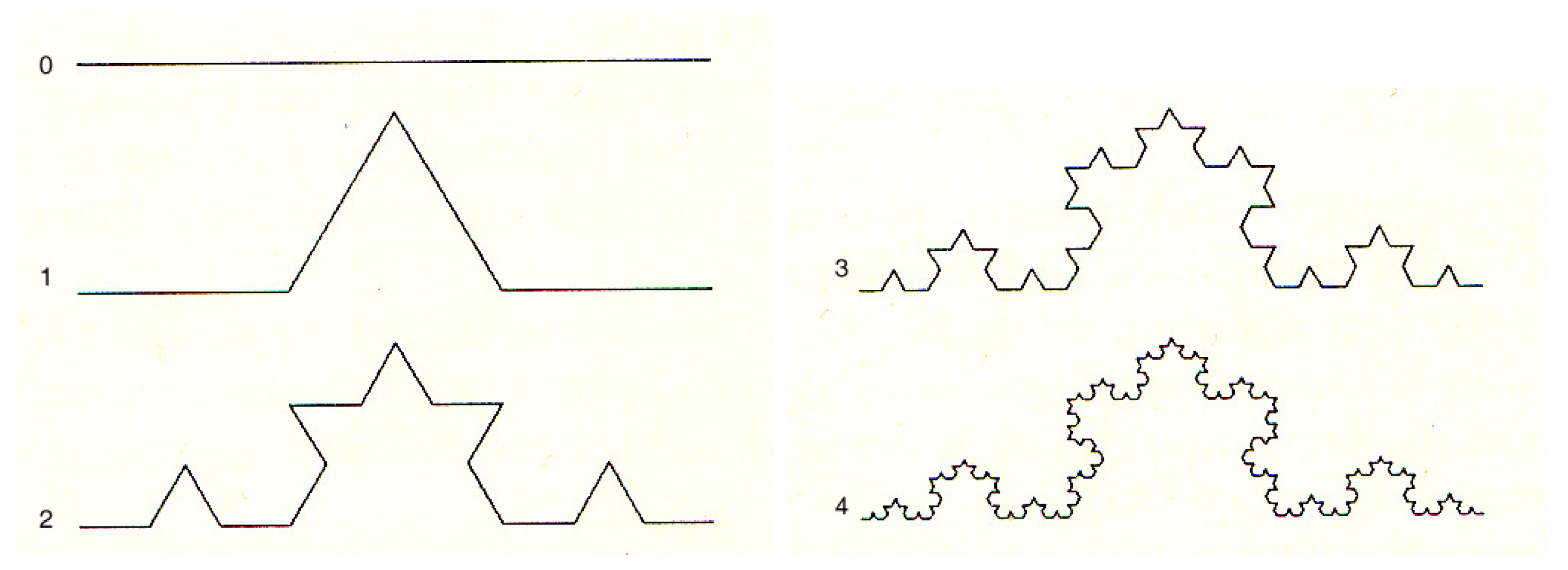
Extension of the discussion to other fractals is possible. For example, for the Koch curve (Figure 2), by using $q=e^{-d\theta }$, with d the fractal dimension, the self-similarity equation $q\alpha =1$ can be written in polar coordinates and is similar to Equation (40) [42]. Then the equations in the z-plane can be written also for the case of the Koch fractal as done for the logarithmic spiral.

I also remark that the system (44) and (45) is isomorph to QED under proper conditions [43]. I will not discuss this issue for brevity.

Taken separately, the damped and amplified oscillators (44) and (45) are open, “non-hamiltonian” systems. However, together they constitute a closed system and the canonical formalism can be used for their analysis [47]. The inclusion in the discussion of both components of the basis $\{e^{-d\theta },e^{+d\theta }\}$ is thus justified also on a physical ground.

This leads us to the discussion of the QFT formalism for dissipative systems. The closed system is found to evolve in time going through the uir of CCR, built on $SU(1,1)$ squeezed coherent states, which are also entangled states. Coherence, dissipation and entanglement thus appear to be interconnected dynamical features of fractal structures.

To see this, starting from the oscillator modes $z_1$ and $z_2$, the operators a and b and their CCR, $[a,a^{†}]=1=[b,b^{†}],[a,b]=0=[a,b^{†}]$, can be introduced in a standard way (I omit for simplicity the momentum subscript k). It is then convenient to define the operators $A=(1/\sqrt{2})(a+b)$ and $B=(1/\sqrt{2})(a-b)$. They annihilate the vacuum $|0\rangle$, $A|0\rangle =0$ and $B|0\rangle =0$, with $|0\rangle \equiv |0\rangle \otimes |0\rangle$, and have CCR. For details see [46,47,48].

From the algebraic point of view, one considers the two oscillators together by introducing the maps $H_F\to H_F\otimes H_F$ and $\mathcal{A}\to \mathcal{A}\otimes \mathcal{A}$, which indeed “duplicates” the algebra $\mathcal{A}$ (the doubling of the degrees of freedom). We thus consider the Hopf algebra with commutative coproduct map $\Delta A=A\otimes \mathbf{1}+\mathbf{1}\otimes A$. One might be interested, however, in making a distinction between the two systems, for example considering one of them as the environment in which the other one is embedded. It is then convenient to move to the “q-deformed” Hopf algebra, with coproduct $\Delta A=A\otimes q+q^{-1}\otimes A$, which is now a non-commutative algebra (under exchange $1\leftrightarrow 2$), and is therefore able to distinguish between “the system” and “its environment” (of course, it is our choice to define which one in the couple is “the system”). In full generality, the q-deformation parameter is $q=e^{\theta }$ or $q=e^{i\theta }$, for bosons or fermions, respectively (see [35,49,50] for details). The non-commutative character of deformed Hopf algebra is also at the root of non-commutative geometry, of which here for brevity I do not report [51], and of the possibility to “label” the uir by using $lnq=\zeta$. Of particular interest is the case of time-dependent q, as it happens indeed with $\zeta =\Gamma t$. Let $\left|0\right(t)\rangle$ denote the vacuum state at t. The time evolution operator is

$$\begin{array}{c}\hfill \mathcal{U}\left(t\right)=exp\left(-\frac{\Gamma t}{2}\left(\left(a^2-a^{†2}\right)-\left(b^2-b^{†2}\right)\right)\right).\end{array}$$

(47)

$\mathcal{U}\left(t\right)$ is also the two mode squeezing operator [47]. In terms of the operators A and B, restoring the k subscript, $\mathcal{U}\left(t\right)$ is

$$\begin{array}{c}\hfill \mathcal{U}\left(t\right)=\prod _{k}exp\left({\Gamma }_{k}t\left(A_k^{†}{B}_k^{†}-A_k{B}_k\right)\right),\end{array}$$

(48)

where we recognize the interaction part $H_I$ of the total Hamiltonian $H=H_0+H_I$ [47],

$$\begin{array}{c}\hfill H_0=\sum _k[\hslash \mathsf{\Omega }(A_k^{†}{A}_k-B_k^{†}{B}_k)+i\hslash \Gamma (A_k^{†}{B}_k^{†}-A_k{B}_k)].\end{array}$$

(49)

Omitting again for simplicity the k subscript, and putting $K_{+}=A^{†}{B}^{†},K_{-}=K_{+}^{†}=AB$, $K_3=(1/2)$$(A^{†}A+B^{†}B+1),$ with the Casimir operator ${\mathcal{C}}^2=(1/4){(A^{†}A-B^{†}B)}^2$, we recognize in H the generators of the $su(1,1)$ algebra: $[K_{+},K_{-}]=-2K_3,[K_3,K_{\pm }]=\pm K_{\pm }$. We also see that $[H_0,H_I]=0$; thus, the condition of positiveness imposed on eigenvalues of $H_0$ is preserved under time evolution induced by $H_I$ ($\mathcal{U}\left(t\right)=e^{-i(t/\hslash )H_I}$).

We also have

$$\begin{array}{ccc}\hfill A_k\to A_k\left(t\right)& =& e^{-i(t/\hslash )H_I}{A}_k{e}^{i(t/\hslash )H_I}=A_{k}cosh\left({\Gamma }_{k}t\right)-B_k^{†}sinh\left({\Gamma }_{k}t\right)\hfill \end{array}$$

(50)

$$\begin{array}{ccc}\hfill B_k\to B_k\left(t\right)& =& e^{-i(t/\hslash )H_I}{B}_k{e}^{i(t/\hslash )H_I}=B_{k}cosh\left({\Gamma }_{k}t\right)-A_k^{†}sinh\left({\Gamma }_{k}t\right)\hfill \end{array}$$

(51)

and h.c., which are the Bogoliubov transformations and give the (inverted) dynamical map of $A\left(t\right)$ and $B\left(t\right)$ in terms of A and B (playing the role of Heisenberg fields). $A\left(t\right)$ and $B\left(t\right)$ annihilate $\left|0\right(t)\rangle$, whose explicit expression is

$$\begin{array}{c}\hfill |0\left(t\right)\rangle =\prod _k\frac{1}{cosh\left({\Gamma }_{k}t\right)}exp\left(tanh\left({\Gamma }_{k}t\right)A_k^{†}{B}_k^{†}\right)|0\rangle ,\end{array}$$

(52)

normalized at each t, $\langle 0\left(t\right)\left|0\right(t)\rangle =1$, and we have

$$\underset{t\to \infty }{lim}\langle 0\left(t\right)|0\rangle \propto \underset{t\to \infty }{lim}exp(-\sum _k{\Gamma }_{k}t)=0,$$

(53)

with ${\sum }_k{\Gamma }_k$ finite and positive, which express the dissipative character (instability) of the oscillators. The B modes represent the heat bath of the A-oscillator [47]. Moreover, destruction of A modes is equivalent to creation of B modes. We have

$$\langle 0\left(t\right)|0\rangle \to 0\mathrm{as}V\to \infty \forall t,$$

(54)

$$\langle 0\left(t\right)|0\left(t^{\prime }\right)\rangle \to 0\mathrm{as}V\to \infty \forall t\mathrm{and}{t}^{\prime },t^{\prime }\ne t$$

(55)

for $\int d^3\kappa {\Gamma }_{\kappa }$ finite and positive. These equations show that the representation $\left\{\right|0\left(t\right)\rangle \}$ is unitarily inequivalent to other representations $\left\{\right|0\left(t^{\prime }\right)\rangle ,\forall t^{\prime }\ne t\}$ in the $V\to \infty$ limit. This confirms that time evolution occurs over trajectories in the manifold of uir. This is a symplectic, Kählerian manifold [28] and trajectories through it can be shown to be classical chaotic ones [52,53].

Time evolution is also controlled by the entropy variations $dS$, which is to be expected due to the dissipative character of the dynamics [42,47]. Heat dissipation is $dQ=(1/\beta )dS$ [47]. The Hamiltonian H can be shown to be actually the free energy $\mathcal{F}=U-TS$. Putting the Boltzmann constat $k_B=1$, the temperature is $T=\hslash \Gamma$, the entropy $S=2K_2$, with $K_2\equiv -(i/2)(K_{+}-K_{-})$, and heat contribution is $2\hslash \Gamma K_2$. It is $T\propto \hslash \mathsf{\Omega }/2$, the zero point energy [8,54]. $\left|0\right(t)\rangle$ is shown to be a finite temperature state in the Thermo Field Dynamics formalism [6,8,47]. This is a remarkable feature since it shows how temperature enters in the dissipative evolution of coherent condensate patterns. One finds

$${\mathcal{N}}_{A_k}\left(t\right)=\langle 0\left(t\right)|A_k^{†}{A}_k|0\left(t\right)\rangle =\langle 0\left(t\right)|B_k\left(t\right)B_k^{†}\left(t\right)|0\left(t\right)\rangle ={sinh}^2{\Gamma }_{k}t,$$

(56)

which gives the number of $A_k$-modes condensed in $\left|0\right(t)\rangle$ at t. Minimizing the free energy gives the Bose-Einstein distribution for ${\mathcal{N}}_{A_k}$ [47].

Equation (56) shows that the q parameter controls the coherent condensate content of $\left|0\right(t)\rangle$. It is remarkable that time for the A-mode is measured by its double B-mode. Notice indeed that in computing ${\mathcal{N}}_{A_k}\left(t\right)$ the only non-vanishing contributions are given by the $B_k\left(t\right)$-modes.

Equation (56) also suggests that A and B are entangled modes [42,53,55]. The $SU(1,1)$ state $\left|0\right(t)\rangle$ is in fact known to be an entangled state for its two mode components. One may compute the linear correlation coefficient $J(N_A,N_B)$ [53,55] and show that the phase-mediated correlation between $A_k$ and $B_k$ modes acquires the maximal value:

$$J(N_A,N_B)=\frac{cov(N_A,N_B)}{{\left(\langle {(\Delta N_A)}^2\rangle \right)}^{1/2}{\left(\langle {(\Delta N_B)}^2\rangle \right)}^{1/2}}=1,$$

(57)

where I have omitted the subscripts k for simplicity. Number operators are denoted by $N_A\equiv N_{A_k}=A_k^{†}{A}_k$, $N_B\equiv N_{B_k}=B_k^{†}{B}_k$. The variance is $\langle {(\Delta N)}^2\rangle \equiv \langle {(N-\langle N\rangle )}^2\rangle =\langle N^2\rangle -{\langle N\rangle }^2$, and the covariance is denoted by $cov(N_A,N_B)\equiv \langle N_A{N}_B\rangle -\langle N_A\rangle \langle N_B\rangle$. The expectation value in $\left|0\right(t)\rangle$ is denoted by $\langle \ast \rangle$.

$\langle N_A{N}_B\rangle =\langle N_A\rangle \langle N_B\rangle$ for non-correlated modes and the covariance is zero. On the contrary, the coherent structure of the vacuum $\left|0\right(t)\rangle$ generates the strong $(A,B)$-pair correlation. Clearly, there is no signal transmission between A and B mode, they are entangled by sharing their common phase in the $\left|0\right(t)\rangle$ condensate. No contradiction arises, therefore, with the relativity principle (and causality), since there is no exchange of messengers among them and, on the another hand, in contrast with the group velocity which is bounded by the speed of light c, the phase velocity is not bounded by c. There are no “spooky force at a distance”. The condensate is a realistic quantum system of entangled modes, observable in its macroscopic manifestation (as realistic is, e.g., a magnet, a crystal, etc.).

I remark that the classical oscillators considered above provide an example of deterministic systems à la ’t Hooft. Quantization emerges when a constraint of the form $K_2|0\rangle =0$ is imposed on physical states. For details see [54,56,57].

Let me finally observe that in the dissipative dynamics discussed above we have a spontaneous breakdown of time translational symmetry and at once breakdown of time-reversal symmetry (cf. Equation (53)). The symmetry of the Hamiltonian (49) under transformations induced by the $K_2$ generator of $SU(1,1)$ is broken in the system vacuum $|0\rangle$ (cf. Equations (54) and (55)). Since $K_2$ is part of the Hamiltonian ($K_2\propto H_I$) we have the breakdown of the “external” (time-)symmetry. In a relativistic system this would correspond to the breakdown of Lorentz time translational symmetry. This is particularly interesting since it happens indeed in the case of quantization in the presence of curved background (the breakdown of Poincaré symmetry) [58] and in the case of vacuum structure in inflationary scenarios in cosmology [59,60,61]. On the other hand, breakdown of time-reversal symmetry involves group contraction mechanisms and can be described in terms of loop–antiloop symmetry [62]. An interesting question is how to extend these results to a general covariant theory [63,64]. From our discussion, one might be tempted to propose gravitational effects as collective modes, macroscopic quantum manifestations of a basic quantum coherent dynamics. The possibility to describe the CMB (cosmic microwave background) in terms of a coherent codensate has been presented in [65]. However, this is a too long story to be further discussed here.

Returning to the discussion of fractals, the conclusion is that fractal forms emerge as macroscopic manifestations of the underlying coherent quantum dynamics (morphogenesis) and their evolution (metamorphoses) goes along trajectories through uir of the CCR. Changes in boundary conditions may turn in diverging trajectories (non-linear dynamical evolution [66]).

9. Conclusions

Some light on the “question of metamorphosis” is shed by the two-level language of QFT. The dynamics of elementary components manifests itself as a flow of evolving forms at the physical level.

Coherent condensation of quanta of long-range correlation waves (the NG boson quanta) determines specific forms, self-similar fractal structures, their evolution and fractal dimension, the vacuum structure.

I have explicitly discussed the example of the ferromagnet. The dynamical rearrangement of symmetry $SU\left(2\right)\to E\left(2\right)$ describes formally the metamorphosis process leading from the collection of randomly oriented spin elements ($SU\left(2\right)$ symmetry) to the organized form of the ferromagnet (on average, a prevalence of, e.g., spin up with respect to spin down).

Changes in the magnetization M are changes in the forms of the ferromagnetic ordered patterns, i.e., further metamorphosis processes evolving in time over classical chaotic trajectories through physically different representations.

The dynamical rearrangement of symmetry is controlled by the Inönü–Wigner group contraction. This is a general result in SBS. It can be shown also by use of projective geometry arguments [67,68] and it has been proved in models invariant under $SU\left(n\right)$, $SO\left(n\right)$, chiral $SU\left(2\right)\times SU\left(2\right)$, $SU\left(3\right)\times SU\left(3\right)$, spontaneous breakdown of phase, chiral phase and scale invariance, the case of a scalar isotriplet, the $SU\left(3\right)$ group in $T-t$ Jahn–Teller systems [25].

The group contraction mechanism introduces translations of the NG fields. These control the coherent boson condensation and thus the formation of ordered patterns. The resulting order parameter is independent of quantum fluctuations due to coherence and thus it is a classical field (of course, far from critical regimes; in polaron theory under boundary conditions of strong coupling the semiclassical limit cannot be achieved [29]). The system then behaves as a macroscopic quantum system, stable under excitations of low momenta NG quanta (the low energy theorems, Section 7).

In Section 6, the intrinsic localized character of physical states and observables has been shown to be at the origin of the dynamical rearrangement of symmetry (the origin of the metamorphosis process). In localized states, infinitesimal contributions of the order of $1/V$, with the volume $V\to \infty$, are missing. The lack of these contributions (the infrared effect) is responsible for the difference between the “rearranged” symmetries and the dynamical ones.

In the discussion on ferromagnets I have considered spontaneous breakdown of “internal” symmetries. Without entering into details, I have only mentioned the breakdown of space translational symmetry (occurring, e.g., in the crystal case). The breakdown of time-reversal symmetry and time translational symmetry has been considered in Section 8. I have not discussed further the breakdown of “external” symmetries. I have only quoted some references on the breakdown of Poincaré symmetry in curved background, the case of inflationary scenarios in cosmology. The question remains open whether the extension of the results to general covariant theories is possible.

SBS is triggered by the coupling of the system with an external agent, e.g., the environment in which it is embedded. Such a coupling, although infinitesimally small ($ϵ\to 0$, Section 3 and Section 4), drives the system to sit in one of the infinitely many uir. The important point is that we deal always with open systems. However, the canonical formalism describes closed systems. Therefore we have to consider the system under study together with its environment. The whole {system-environment} is then a closed system. Through such a doubling of the degrees of freedom, temperature enters in our scheme. Free energy minimization plays then a relevant role and the breakdown of time-reversal symmetry (the arrow of time) makes time evolution irreversible (… perhaps it is not a case that in stories and legends undoing a metamorphosis (break a spell, restore a symmetry) requires a miraculous action…only the kiss of the Princess may reverse the arrow of time and let the frog go back to be the most beautiful Prince [69]).

The modes A and B in the state $\left|0\right(t)\rangle$ are entangled modes (Equation (57)). A and B annihilate the vacuum state $|0\rangle$. They do not annihilate the physical vacuum $\left|0\right(t)\rangle$, which is instead annihilated by the physical modes $A\left(t\right)$ and $B\left(t\right)$. The states $|0\rangle$ and $\left|0\right(t)\rangle$, (and similarly $\left|0\right(t)\rangle$ and $\left|0\right(t^{\prime })\rangle$, for any $t\ne t^{\prime }$) are unitarily inequivalent states (Equations (54) and (55)). The measurement of the number of A modes is actually determined by the $B\left(t\right)$ modes (Equation (56)). The entanglement thus reveals itself when quantities of the “Heisenberg field level” are computed in the “physical level” (the vacuum $\left|0\right(t)\rangle$ at time t) [53]. Equation (56) is an example of computation by use of the dynamical map, expressed in this case by the Bogoliubov transformations (50) and (51) (the number operator of the Heisenberg A field is measured by use of the “lens” of the physical fields $A\left(t\right)$ and $B\left(t\right)$ and physical vacuum $\left|0\right(t)\rangle$).

The QFT formalism and the remarks on the openness of the system apply to condensed matter and particle physics and find wide experimental confirmation. They have been also extended to biology and neuroscience [70,71,72,73,74,75,76,77,78] and to some aspects of linguistics [79] in the generation of meanings, in the transition from syntax to semantics (see also [80,81,82] where the openness of the system also plays a crucial role).

Within the unified vision of nature that then emerges, the realization of the same basic dynamics into many forms depicts in terms of mathematical structures the metamorphosis of the being into the existing, its unfolding in the kaleidoscopic variety of the existence, if I am allowed to use metaphoric images [69,83]. Perhaps, as already done in [46], it might be worth to close by quoting one famous passage by Darwin “ […] in this view of life, with its several powers, having been originally breathed into a few form or into one; […] from so simple a beginning endless forms most beautiful and most wonderful have been, and are being, evolved.” [1].

References

- Darwin, C. On the Origin of Species; John Murray: London, UK, 1860; p. 490. [Google Scholar]
- Schweber, S.S. An Introduction to Relativistic Quantum Field Theory; Harper and Row Publ. Inc.: New York, NY, USA, 1961. [Google Scholar]
- Bogoliubov, N.N.; Logunov, A.A.; Todorov, I.T. Axiomatic Quantum Field Theory; Benjamin: New York, NY, USA, 1975. [Google Scholar]
- Bogoliubov, N.N. Lectures on qUantum Statistics, Quasi-Averages; Macdonald & Co. Ltd.: London, UK, 1971; Volume 2, ISBN 0356026981, ISBN 978-0356026985. [Google Scholar]
- Umezawa, H.; Matsumoto, H.; Tachiki, M. Thermo Field Dynamics and Condensed States; North-Holland: Amsterdam, The Netherlands, 1982. [Google Scholar]
- Umezawa, H. Advanced Field Theory: Micro, Macro and Thermal Concepts; American Institute of Physics: New York, NY, USA, 1993. [Google Scholar]
- Vitiello, G. Dynamical rearrangement of symmetry. Diss. Ab. Intern. 1975, 36/02, 769-B. [Google Scholar]
- Blasone, M.; Jizba, J.; Vitiello, G. Quantum Field Theory and Its Macroscopic Manifestations; Imperial College Press: London, UK, 2011. [Google Scholar]
- Umezawa, H. Developments in concepts in quantum field theory in half century. Math. Jpn. 1995, 41, 109–124. [Google Scholar]
- von Neumann, J. Mathematical Foundations of Quantum Mechanics; Princeton University Press: Princeton, NY, USA, 1955. [Google Scholar]
- Del Giudice, E.; Manka, R.; Milani, M.; Vitiello, G. Non-constant order parameter and vacuum evolution. Phys. Lett. B 1988, 206, 661–664. [Google Scholar] [CrossRef]
- Bratteli, O.; Robinson, D.W. Operator Algebras and Quantum Statistical Mechanics; Springer: Berlin, Germany, 1979. [Google Scholar]
- Vitiello, G. The world opacity and knowledge. In The Systemic Turn in Human and Natural Sciences. The Rock in the Pond; Urbani Ulivi, L., Ed.; Springer Nature Switzerland AG: Cham, Switzerland, 2019; pp. 41–51. (In Italian) [Google Scholar]
- Umezawa, H. Dynamical rearrangement of symmetries. Nuovo Cim. A 1965, 40, 450–475. [Google Scholar] [CrossRef]
- Leplae, L.; Sen, R.N.; Umezawa, H. Asymmetric ground states in invariant many-body theories. Nuovo Cim. B 1967, 49, 1–31. [Google Scholar] [CrossRef]
- Matsumoto, H.; Umezawa, H.; Vitiello, G.; Wyly, J.K. Spontaneous breakdown of a non-Abelian symmetry. Phys. Rev. D 1974, 9, 2806–2813. [Google Scholar] [CrossRef]
- Shah, M.N.; Umezawa, H.; Vitiello, G. Relation among spin operators and magnons. Phys. Rev. B 1974, 10, 4724–4726. [Google Scholar] [CrossRef]
- Shah, M.N.; Vitiello, G. Self-consistent formulation of itinerant electron ferromagnet. Nuovo Cim. B 1975, 30, 21–42. [Google Scholar] [CrossRef]
- De Concini, C.; Vitiello, G. Spontaneous breakdown of symmetry and group contraction. Nucl. Phys. B 1976, 116, 141–156. [Google Scholar] [CrossRef]
- Celeghini, E.; Graziano, E.; Vitiello, G. Classical limit and spontaneous breakdown of symmetry as an environment effect in quantum field theory. Phys. Lett. A 1990, 145, 1–6. [Google Scholar] [CrossRef]
- Goldstone, J.; Salam, A.; Weinberg, S. Broken Symmetries. Phys. Rev. 1962, 127, 965–970. [Google Scholar] [CrossRef]
- Inönü, E.; Wigner, E.P. On the contraction of groups and their representations. Proc. Nat. Acad. Sci. USA 1953, 39, 510–524. [Google Scholar] [CrossRef] [PubMed] [Green Version]
- Segal, I.E. A class of operator algebras which are determined by groups. Duke Math. J. 1951, 18, 221–265. [Google Scholar] [CrossRef]
- Saletan, E.J. Contraction of Lie groups. J. Math. Phys. 1961, 2, 1–21. [Google Scholar] [CrossRef]
- Vitiello, G. Dynamical rearrangement of SU(3) symmetry. Phys. Lett. A 1976, 58, 293–294. [Google Scholar] [CrossRef]
- Weimar, E. What does the centre of the universal enveloping algebra tell us about the deformations of representations? Nuovo Cim. 1973, 15, 245–256. [Google Scholar] [CrossRef]
- Klauder, J.R.; Sudarshan, E.C.G. Fundamentals of Quantum Optics; Benjamin: New York, NY, USA, 1968. [Google Scholar]
- Perelomov, A. Generalized Coherent States and Their Applications; Springer: Berlin, Germany, 1986. [Google Scholar]
- Lakhno, V.D. Translation-invariant bipolarons and superconductivity. Condens. Matter 2020, 5, 30. [Google Scholar] [CrossRef]
- Higgs, P.W. Spontaneous Symmetry Breakdown without Massless Bosons. Phys. Rev. 1966, 145, 1156–1163. [Google Scholar] [CrossRef] [Green Version]
- Kibble, T.W.B. Symmetry breaking in nonAbelian gauge theories. Phys. Rev. 1967, 155, 1554–1561. [Google Scholar] [CrossRef]
- Matsumoto, H.; Papastamatiou, N.J.; Umezawa, H.; Vitiello, G. Dynamical rearrangement in Anderson-Higgs-Kibble mechanism. Nucl. Phys. B 1975, 97, 61–89. [Google Scholar] [CrossRef]
- Vitiello, G. Topological defects, fractals and the structure of quantum field theory. In Vision of Oneness; Licata, I., Sakaji, A.J., Eds.; Aracne Edizioni: Rome, Italy, 2011; pp. 155–180. [Google Scholar]
- Celeghini, E.; De Martino, S.; De Siena, S.; Rasetti, M.; Vitiello, G. Quantum groups, squeezing, Bloch and theta functions. Mod. Phys. Lett. B 1993, 7, 1321–1329. [Google Scholar] [CrossRef]
- Celeghini, E.; De Martino, S.; De Siena, S.; Rasetti, M.; Vitiello, G. Quantum groups, coherent states, squeezing, and lattice quantum mechanics. Ann. Phys. 1995, 241, 50–67. [Google Scholar] [CrossRef] [Green Version]
- Holstein, T.; Primakoff, H. Field Dependence of the Intrinsic Domain Magnetization of a Ferromagnet. Phys. Rev. 1940, 58, 1098–1113. [Google Scholar] [CrossRef]
- Umezawa, H.; Vitiello, G. Quantum Mechanics; Bibliopolis: Napoli, Italy, 1985. [Google Scholar]
- Alfinito, E.; Vitiello, G. Formation and life-time of memory domains in the dissipative quantum model of brain. Int. J. Mod. Phys. B 2000, 14, 853–868. [Google Scholar] [CrossRef] [Green Version]
- Dyson, F.J. General Theory of Spin-Wave Interactions. Phys. Rev. 1956, 102, 1217–1230. [Google Scholar] [CrossRef]
- Adler, S.L. Consistency Conditions on the Strong Interactions Implied by a Partially Conserved Axial-Vector Current. II. Phys. Rev. B 1965, 139, 1638–1643. [Google Scholar] [CrossRef]
- Vitiello, G. Coherent states, fractals and brain waves. New Math. Nat. Comput. 2009, 5, 245–264. [Google Scholar] [CrossRef] [Green Version]
- Vitiello, G. Fractals, coherent states and self-similarity induced noncommutative geometry. Phys. Lett. A 2012, 376, 2527–2532. [Google Scholar] [CrossRef] [Green Version]
- Vitiello, G. On the isomorphism between dissipative systems, fractal self-similarity and electrodynamics. Toward an integrated vision of nature. Systems 2014, 2, 203–216. [Google Scholar] [CrossRef]
- Peitgen, H.O.; Jürgens, H.; Saupe, D. Chaos and Fractals. New frontiers of Science; Springer: Berlin, Germany, 1986. [Google Scholar]
- Bunde, A.; Havlin, S. (Eds.) Fractals in Science; Springer: Berlin, Germany, 1995. [Google Scholar]
- Vitiello, G. …And Kronos ate his sons. In Beyond Peaceful Coexistence. The Emergence of Space, Time and Quantum; Licata, I., Ed.; Imperial College Press: London, UK, 2016; pp. 465–486. [Google Scholar]
- Celeghini, E.; Rasetti, M.; Vitiello, G. Quantum Dissipation. Ann. Phys. 1992, 215, 156–170. [Google Scholar] [CrossRef]
- Vitiello, G. Links. Relating different physical systems through the common QFT algebraic structure. In Quantum Analogues: From Phase Transitions to Black Holes and Cosmology; Lectures Notes in Physics 718; Unruh, W.G., Schuetzhold, R., Eds.; Springer: Berlin, Germany, 2007; pp. 165–205. [Google Scholar]
- Celeghini, E.; Rasetti, M.; Vitiello, G. Squeezing and Quantum Groups. Phys. Rev. Lett. 1991, 66, 2056–2059. [Google Scholar] [CrossRef] [PubMed]
- Celeghini, E.; De Martino, S.; De Siena, S.; Iorio, A.; Rasetti, M.; Vitiello, G. Thermo field dynamics and quantum algebras. Phys. Lett. A 1998, 244, 455–461. [Google Scholar] [CrossRef] [Green Version]
- Sivasubramanian, S.; Srivastava, Y.N.; Vitiello, G.; Widom, A. Quantum dissipation induced noncommutative geometry. Phys. Lett. A 2003, 311, 97–105. [Google Scholar] [CrossRef] [Green Version]
- Vitiello, G. Classical chaotic trajectories in quantum field theory. Int. J. Mod. Phys. B 2004, 18, 785–792. [Google Scholar] [CrossRef] [Green Version]
- Sabbadini, S.A.; Vitiello, G. Entanglement and phase-mediated correlations in quantum field theory. Application to brain-mind states. Appl. Sci. 2019, 9, 3203. [Google Scholar] [CrossRef] [Green Version]
- Blasone, M.; Jizba, P.; Vitiello, G. Dissipation and quantization. Phys. Lett. A 2001, 287, 205–210. [Google Scholar] [CrossRef] [Green Version]
- Gerry, C.C.; Knight, P.L. Introductory Quantum Optics; Cambridge University Press: Cambridge, UK, 2005. [Google Scholar]
- Hooft, G.T. Quantum gravity as a dissipative deterministic system. Class. Quant. Grav. 1999, 16, 3263–3279. [Google Scholar] [CrossRef] [Green Version]
- Hooft, G.T. A mathematical theory for deterministic quantum mechanics. J. Phys. Conf. Ser. 2007, 67, 012015. [Google Scholar] [CrossRef]
- Martellini, M.; Sodano, P.; Vitiello, G. Vacuum Structure for a Quantum Field Theory in Curved Space-Time. Nuovo Cim. A 1978, 48, 341–358. [Google Scholar] [CrossRef]
- Alfinito, E.; Vitiello, G. Canonical quantization and expanding metrics. Phys. Lett. A 1999, 252, 5–10. [Google Scholar] [CrossRef] [Green Version]
- Alfinito, E.; Vitiello, G. Vacuum structure for expanding geometry. Class. Quant. Grav. 2000, 17, 93–111. [Google Scholar] [CrossRef]
- Alfinito, E.; Vitiello, G. Double universe and the arrow of time. J. Phys. Conf. Ser. 2007, 67, 012010. [Google Scholar] [CrossRef]
- Alfinito, E.; Vitiello, G. Time reversal violation as loop-antiloop symmetry breaking: The Bessel equation, group contraction and dissipation. Mod. Phys. Lett. B 2003, 17, 1–12. [Google Scholar] [CrossRef]
- Hooft, G.T. Foreword. In Beyond Peaceful Coexistence. The Emergence of Space, Time and Quantum; Licata, I., Ed.; Imperial College Press: London, UK, 2016; pp. ix–x. [Google Scholar]
- Licata, I. From peaceful coexistence to co-emergence. In Beyond Peaceful Coexistence. The Emergence of Space, Time and Quantum; Licata, I., Ed.; Imperial College Press: London, UK, 2016; pp. xi–xx. [Google Scholar]
- Capolupo, A.; Lambiase, G.; Vitiello, G. Thermal Condensate Structure and Cosmological Energy Density of the Universe. Adv. High Energy Phys. 2016, 2016, 3127597. [Google Scholar] [CrossRef] [Green Version]
- Hilborn, R. Chaos and Nonlinear Dynamics; Oxford University Press: Oxford, UK, 1994. [Google Scholar]
- De Concini, C.; Vitiello, G. Relation between projective geometry and group contraction in spontaneously broken symmetry theories. Phys. Lett. B 1977, 70, 355–357. [Google Scholar] [CrossRef]
- Celeghini, E.; Magnollay, P.; Tarlini, M.; Vitiello, G. Non linear realizations and contraction of group representations. Phys. Lett. B 1985, 162, 133–136. [Google Scholar] [CrossRef]
- Vitiello, G. Simmetrie e metamorfosi. Atque 2019, 24, 139–160. [Google Scholar]
- Del Giudice, E.; Doglia, S.; Milani, M.; Vitiello, G. A quantum field theoretical approach to the collective behavior of biological systems. Nucl. Phys. B 1985, 251, 375–400. [Google Scholar] [CrossRef]
- Del Giudice, E.; Doglia, S.; Milani, M.; Vitiello, G. Electromagnetic field and spontaneous symmetry breakdown in biological matter. Nucl. Phys. B 1986, 275, 185–199. [Google Scholar] [CrossRef]
- Vitiello, G. Dissipation and memory capacity in the quantum brain model. Int. J. Mod. Phys. B 1995, 9, 973–989. [Google Scholar] [CrossRef]
- Loppini, A.; Capolupo, A.; Cherubini, C.; Gizzi, A.; Bertolaso, M.; Filippi, S.; Vitiello, G. On the coherent behavior of pancreatic beta cell clusters. Phys. Lett. A 2014, 378, 3210–3217. [Google Scholar] [CrossRef] [Green Version]
- Vitiello, G. My Double Unveiled; John Benjamins: Amsterdam, The Netherlands, 2001. [Google Scholar]
- Freeman, W.J.; Vitiello, G. Nonlinear brain dynamics as macroscopic manifestation of underlying many-body dynamics. Phys. Life Rev. 2006, 3, 93–117. [Google Scholar] [CrossRef] [Green Version]
- Freeman, W.J.; Vitiello, G. Matter and Mind are entangled in two streams of images guiding behavior and informing the subject through awareness. Mind Matter 2016, 14, 7–24. [Google Scholar]
- Kurian, P.; Capolupo, A.; Craddock, T.J.A.; Vitiello, G. Water-mediated correlations in DNA-enzyme interactios. Phys. Lett. A 2016, 382, 33–43. [Google Scholar] [CrossRef] [PubMed]
- Montagnier, L.; Aïssa, J.; Capolupo, A.; Craddock, T.J.A.; Kurian, P.; Lavallee, C.; Polcari, A.; Romano, P.; Tedeschi, A.; Vitiello, G. Water bridging dynamics of polymerase chain reaction in the gauge theory paradigm of quantum fields. Water 2017, 9, 339, Addendum 9, 436. [Google Scholar] [CrossRef]
- Piattelli-Palmarini, M.; Vitiello, G. Linguistics and Some Aspects of Its Underlying Dynamics. Biolinguistics 2015, 9, 96–115. [Google Scholar]
- Longo, G. Confusing biological rhythms and physical clocks. Today’s ecological relevance of Bergson-Einstein debate on time. In Proceedings of the Conference “What is time? Einstein and Bergson 100 years later”, L’Aquila, Italy, 4–6 April 2019. in press. [Google Scholar]
- Damasco, A.; Giuliani, A. A resonance based model of biological evolution. Physics A 2017, 471, 750–756. [Google Scholar] [CrossRef]
- Camponeschi, I.; Damasco, A.; Uversky, V.N.; Giuliani, A.; Bianchi, M.M. Phenotypic suppression caused by resonance with light-dark cycles indicates the presence of a 24-h oscillator in yeast and suggests a new role of intrinsically disordered protein regions as internal mediators. J. Biomol. Struct. Dyn. 2020, accepted. [Google Scholar] [CrossRef]
- Fadini, U.; Pieri, P.F. (Eds.) Prefazione. In Metamorfosi Del Vivente. Atque; Moretti & Vitali: Bergamo, Italy, 2019; Volume 24, pp. 9–17. [Google Scholar]
Figure 1.
Anti-clockwise and clockwise logarithmic spirals.
Figure 2.
First five stages of the Koch curve.
© 2020 by the author. Licensee MDPI, Basel, Switzerland. This article is an open access article distributed under the terms and conditions of the Creative Commons Attribution (CC BY) license (http://creativecommons.org/licenses/by/4.0/).
Share and Cite
MDPI and ACS Style
Vitiello, G. Symmetries and Metamorphoses. Symmetry 2020, 12, 907. https://0-doi-org.brum.beds.ac.uk/10.3390/sym12060907
AMA Style
Vitiello G. Symmetries and Metamorphoses. Symmetry. 2020; 12(6):907. https://0-doi-org.brum.beds.ac.uk/10.3390/sym12060907
Chicago/Turabian StyleVitiello, Giuseppe. 2020. "Symmetries and Metamorphoses" Symmetry 12, no. 6: 907. https://0-doi-org.brum.beds.ac.uk/10.3390/sym12060907
Note that from the first issue of 2016, this journal uses article numbers instead of page numbers. See further details here.