On the Analytical and Numerical Study of a Two-Dimensional Nonlinear Heat Equation with a Source Term

Abstract

The paper deals with two-dimensional boundary-value problems for the degenerate nonlinear parabolic equation with a source term, which describes the process of heat conduction in the case of the power-law temperature dependence of the heat conductivity coefficient. We consider a heat wave propagation problem with a specified zero front in the case of two spatial variables. The solution existence and uniqueness theorem is proved in the class of analytic functions. The solution is constructed as a power series with coefficients to be calculated by a proposed constructive recurrent procedure. An algorithm based on the boundary element method using the dual reciprocity method is developed to solve the problem numerically. The efficiency of the application of the dual reciprocity method for various systems of radial basis functions is analyzed. An approach to constructing invariant solutions of the problem in the case of central symmetry is proposed. The constructed solutions are used to verify the developed numerical algorithm. The test calculations have shown the high efficiency of the algorithm.

1. Introduction

We consider a quasilinear parabolic equation in the case of power-law nonlinearity, which models the heat conduction process:

$$T_t=\mathsf{\alpha }\mathrm{div}\left(T^{\mathsf{\sigma }} \nabla T\right)+\mathrm{H}\left(T\right).$$

(1)

Here, $t$ is time, $T$ is the required function (temperature), $\mathsf{\alpha }$, $\mathsf{\sigma }$ are positive constants, $\mathrm{H}\left(T\right)$ is a specified source function, and $\mathrm{H}\left(0\right)=0$, $\mathrm{div}$, $\nabla$ are spatial divergence and spatial gradient.

Equation (1) is the complete form of the porous medium equation [1]. Besides heat conduction, Equation (1) describes polytropic gas filtration in a porous medium [2,3,4] and diffusion.

By the standard substitution, $u=T^{\mathsf{\sigma }}, t^{\prime }=\mathsf{\alpha }t$, Equation (1) is reduced to the equation

$$u_t=u\Delta u+\frac{1}{\mathsf{\sigma }}{\left(\nabla u\right)}^2+\mathsf{\eta }\left(u\right),$$

(2)

where $\mathsf{\eta }\left(u\right)=\frac{\mathsf{\sigma }}{\mathsf{\alpha }}{u}^{1-\frac{1}{\mathsf{\sigma }}}\mathrm{H}\left(u^{\frac{1}{\mathsf{\sigma }}}\right)$. It is assumed that the source function is such that $\mathsf{\eta }\left(0\right)=0$. This is always true when $\mathsf{\sigma }>1$.

Proceeding from the physical meaning of the problem, we consider only the values $u\ge 0$ and $T\ge 0$. When $u>0$ and $T>0$, it is clear that Equations (1) and (2), are equivalent. If, simultaneously, $T=0$ and $T^{\mathsf{\sigma }}=0$, which is always true when $\mathsf{\sigma }>0$, there is one-to-one correspondence between the values of the functions $u$ and $T$; however, the properties of the derivatives need to be further investigated.

It is Equation (2) that will be studied in what follows. Note that its characteristic feature is parabolic-type degeneration when $u=0$, since the factor in front of the Laplacian in the right-hand side becomes zero. For the solutions of Equation (2), this results in the appearance of the degeneration of some properties in the neighborhood of a line (point, surface), which are generally typical of hyperbolic equations. One of these properties is that Equation (2) has heat-wave (filtration-wave) type solutions, which can be constructed as special series [4,5]. Note that the study of degenerate partial differential and integro-differential equations applicable to mathematical physics and mechanics has received much attention from researchers in the school of thought headed by N. A. Sidorov [6], including proving theorems of the existence and uniqueness of classical [7] and generalized [8] solutions.

It is well known that analytical methods in solving nonlinear problems of mathematical physics are rather poorly applicable. Thus, all the above-mentioned existence and uniqueness theorems are local. In this respect, it is expedient to complement the analytical study by a numerical one.

The dual reciprocity boundary element method (DRBEM), first proposed in [9] for solving nonstationary heat conduction problems, is an effective means of solving boundary value problems for various parabolic equations, namely heat conduction [10,11,12], diffusion [13], advection–diffusion [14], convection–diffusion–reaction [15,16], etc. The common approach in these studies is the representation of the parabolic equation as an inhomogeneous Poisson equation with a time derivative in the right-hand part and the application of the boundary element method (BEM) to solving the obtained elliptic equation. An important role in applying the dual reciprocity method (DRM) is played by the choice of the form of radial basis functions [17,18]. When nonlinear problems are solved by the boundary element method [11,12,13], the DRM allows domain integrals to be reduced to boundary integrals, and this reduces the problem dimension, the subsequent solution being determined by the chosen time-stepping scheme. A similar approach was proposed by us in [19,20] for solving problems with a moving boundary for the degenerate nonlinear parabolic equation. In the present paper, this approach is extended to the numerical solution of a two-dimensional nonlinear equation with a source term.

Unfortunately, for approximate methods of constructing solutions to boundary value problems for nonlinear equations of mathematical physics, it is very seldom possible to prove any rigorous statements of convergence, excluding statements of the local convergence of power series [21]. An important tool for the verification of calculation results under these conditions is a comparison with exact solutions [22], their construction being often reduced to the integration of ordinary differential equations [23]. To study the properties of heat waves, exact solutions, in particular, enable one to go beyond the small neighborhood in which it is generally possible to prove the series convergence [24]. In the theory of blow-up regimes, developed by the researchers in Samarsky’s school of thought, exact solutions are used as illustrative examples [25]. New classes of wave-type exact solutions to the nonlinear heat conduction equation without sources (sinks) were obtained in [26], their construction being reducible to the integration of the Cauchy problems for the generalized Liénard equation [27,28].

2. The Existence and Uniqueness Theorem

We write Equation (2) for the two-dimensional case in the polar coordinates $\mathsf{\rho }$, $\mathsf{\phi }$ as

$$u_t=u{u}_{\mathsf{\rho }\mathsf{\rho }}+\frac{u_{\mathsf{\rho }}^2}{\mathsf{\sigma }}+\frac{u{u}_{\mathsf{\rho }}}{\mathsf{\rho }}+\frac{1}{{\mathsf{\rho }}^2}\left(\frac{u_{\mathsf{\phi }}^2}{\mathsf{\sigma }}+u{u}_{\mathsf{\phi }\mathsf{\phi }}\right)+\mathsf{\eta }\left(u\right),$$

(3)

where $\mathsf{\eta }\left(0\right)=0$. The boundary condition is given as

$${u|}_{\mathsf{\rho }=b\left(t,\mathsf{\phi }\right)}=0.$$

(4)

We formulate and prove the theorem of the existence and uniqueness of a nontrivial solution to the problems (3) and (4) in the class of analytical functions with a simultaneous construction of the solution in the form of a converging power series.

Theorem 1.

Assume that the function $b\left(t,\mathsf{\phi }\right)$ in the problems (3) and (4) possesses the following properties:

• $b\left(t,-\mathsf{\pi }\right)=b\left(t,\mathsf{\pi }\right), b\left(t,\mathsf{\phi }\right)>0$ and $\mathsf{\eta }\left(0\right)=0$.
• $b\left(t,\mathsf{\phi }\right)$ and $1/b\left(t,\mathsf{\phi }\right)$ are analytical with respect to $\mathsf{\phi }$ when $-\mathsf{\pi }\le \mathsf{\phi }\le \mathsf{\pi }$ and, in terms of $t$ in some neighborhood of the initial time $t=0$, $\mathsf{\eta }\left(u\right)$ is analytical with respect to $u$.

Then, the problems (3) and (4) in some neighborhood of the closed line $\mathsf{\rho }=b\left(0,\mathsf{\phi }\right)$, $-\mathsf{\pi }\le \mathsf{\phi }\le \mathsf{\pi }$, has a unique nontrivial analytical solution, local with respect to $t$.

Proof. 

Theorem 1 is proved in two stages as follows: in Stage 1, the solution of the problems (3) and (4) is constructed as a power series with recurrently computed coefficients; in Stage 2, the convergence of the constructed series is proved. □

Stage 1.

Make a substitution of the independent variables in Equation (3),

$$\mathsf{\tau }=t, s=\mathsf{\rho }-b\left(t,\mathsf{\phi }\right), \mathsf{\psi }=\mathsf{\phi }.$$

(5)

With the substitution in (5), the derivatives become as follows: $u_{\mathsf{\rho }}=u_s$, $u_t=u_{\mathsf{\tau }}-b_{\mathsf{\tau }}{u}_s$, $u_{\mathsf{\phi }}=u_{\mathsf{\psi }}-b_{\mathsf{\psi }}{u}_s$, $u_{\mathsf{\rho }\mathsf{\rho }}=u_{ss}$, $u_{\mathsf{\phi }\mathsf{\phi }}=u_{\mathsf{\psi }\mathsf{\psi }}+b_{\mathsf{\psi }}^2{u}_{ss}-b_{\mathsf{\psi }}{u}_{\mathsf{\psi }s}-b_{\mathsf{\psi }\mathsf{\psi }}{u}_s$. Then, Equation (3) becomes

$$\begin{array}{c}{u}_{\mathsf{\tau }}=b_{\mathsf{\tau }}{u}_s+u{u}_{ss}+\frac{u_s^2}{\mathsf{\sigma }}+\frac{u{u}_s}{b+s}\\ +\frac{1}{{\left(b+s\right)}^2}\left[u{u}_{\mathsf{\psi }\mathsf{\psi }}+\frac{u_{\mathsf{\psi }}^2}{\mathsf{\sigma }}-2b_{\mathsf{\psi }}\left(\frac{u_{\mathsf{\psi }}{u}_s}{\mathsf{\sigma }}+u{u}_{\mathsf{\psi }s}\right)+b_{\mathsf{\psi }}^2\left(u{u}_{ss}+\frac{u_s^2}{\mathsf{\sigma }}\right)-u{b}_{\mathsf{\psi }\mathsf{\psi }}{u}_s\right]+\mathsf{\eta }\left(u\right).\end{array}$$

(6)

Transform Equation (6) to a more convenient form by grouping the terms:

$$\begin{array}{c}{u}_{\mathsf{\tau }}=b_{\mathsf{\tau }}{u}_s+B\left(\mathsf{\tau },\mathsf{\psi },s\right)\left(u{u}_{ss}+\frac{u_s^2}{\mathsf{\sigma }}\right)+\frac{1}{b+s}\left(1-\frac{b_{\mathsf{\psi }\mathsf{\psi }}}{b+s}\right)u{u}_s\\ +\frac{1}{{\left(b+s\right)}^2}\left[u{u}_{\mathsf{\psi }\mathsf{\psi }}+\frac{u_{\mathsf{\psi }}^2}{\mathsf{\sigma }}-2b_{\mathsf{\psi }}\left(\frac{u_{\mathsf{\psi }}{u}_s}{\mathsf{\sigma }}+u{u}_{\mathsf{\psi }s}\right)\right]+\mathsf{\eta }\left(u\right).\end{array}$$

(7)

Here, $B\left(\mathsf{\tau },\mathsf{\psi },s\right)=1+b_{\mathsf{\psi }}^2/{\left(b+s\right)}^2$. The boundary condition, (4), can then be written as

$${u|}_{s=0}=0.$$

(8)

The solution to the problems (7) and (8) is constructed in the form of a series with respect to the powers of $s$:

$$u={\displaystyle \sum _{k=0}^{\infty }\frac{u_k\left(\mathsf{\tau },\mathsf{\psi }\right)}{k!}{s}^k},$$

(9)

where $u_k={\frac{{\partial }^{k}u}{\partial s^k}|}_{s=0}$. It follows from the boundary conditions that $u_0\left(\mathsf{\tau },\mathsf{\psi }\right)=0$.

In order to find $u_1$, it is set that $s=0$ in Equation (7). We obtain

$$0=b_{\mathsf{\tau }}{u}_1+\frac{1}{\mathsf{\sigma }}{B}^0{u}_1^2,$$

(10)

where $B^0={B|}_{s=0}$.

Assume that $u_1\ne 0$ (in the opposite case, we have a trivial solution). Then $u_1\left(\mathsf{\tau },\mathsf{\psi }\right)=-\mathsf{\sigma }\mathsf{\beta }\left(\mathsf{\tau },\mathsf{\psi }\right)$, where $\mathsf{\beta }\left(\mathsf{\tau },\mathsf{\psi }\right)=b_{\mathsf{\tau }}\left(\mathsf{\tau },\mathsf{\psi }\right)/B^0\left(\mathsf{\tau },\mathsf{\psi }\right)$. To find $u_2$, we differentiate both sides, set $s=0$ and represent $u_2$ in terms of the known quantities. We arrive at the following:

$$u_2=\frac{u_{1\mathsf{\tau }}+\left[\frac{b_{\mathsf{\psi }\mathsf{\psi }}}{b}-\left(1+\frac{2}{\mathsf{\sigma }}\right)\right]\frac{1}{b}{u}_1^2+\frac{2b_{\mathsf{\psi }}}{b^2}\left(1+\frac{1}{\mathsf{\sigma }}\right)u_1{u}_{1\mathsf{\psi }}-{\mathsf{\eta }}^{\prime }\left(0\right)u_1}{b_{\mathsf{\tau }}+B^0\left(1+\frac{2}{\mathsf{\sigma }}\right)u_1},$$

(11)

and so on. By differentiating Equation (7) $k$ times and setting $s=0$, we have

$$\left[B^0\left(k+\frac{2}{\mathsf{\sigma }}\right)u_1+b_{\mathsf{\tau }}\right]u_{k+1}={\Phi }_k,$$

(12)

where ${\Phi }_k$ depends on the coefficients $u_0$, $u_1$,…, $u_k$ (and their derivatives with respect to $\mathsf{\tau }$, $\mathsf{\psi }$). Being too cumbersome, the expressions for ${\Phi }_k$ are omitted here. It can be easily demonstrated that the multiplier for $u_{k+1}$ in the latter equation is $-\left(k\mathsf{\sigma }+1\right)b_{\mathsf{\tau }}\ne 0$; i.e., all the coefficients of the series represented by Equation (9) are determined uniquely.

Stage 2.

Let us now prove the convergence of the series in Equation (9).

All $u_k\left(\mathsf{\tau },\mathsf{\psi }\right)$ are analytical in some neighborhood of $\mathsf{\tau }=0$ and at all $-\mathsf{\pi }\le \mathsf{\psi }\le \mathsf{\pi }$. This follows from the construction procedure and the theorem conditions; namely, ${\Phi }_k$ denotes analytic functions by construction since they have been obtained from the differentiation of analytical functions; $\left(k\mathsf{\sigma }+1\right)b_{\mathsf{\tau }}\ne 0$ is an analytic function according to condition (2) of the theorem. It also follows from the theorem statement that $\mathsf{\eta }\left(u\right)=u{\mathsf{\eta }}^{*}\left(u\right)$, where ${\mathsf{\eta }}^{*}\left(u\right)$ is a function analytical in the neighborhood of $u=0$.

The proof follows the classical majorant method [2], which is generally applied to proving the Cauchy–Kovalevskaya theorem and its analogs. In this case, the construction of the majorant is complicated by the fact that the equation we have is not the Cauchy–Kovalevskaya type, since it cannot be solved with respect to the highest derivative. In this connection, we first eliminate the singularity by means of partial expansion of the required function in a Taylor series. Then we construct a majorant equation, unsolved with respect to the highest derivative, but already lacking singularity. Finally, we resolve this equation with respect to the highest derivative by differentiating both sides by the variable $s$.

We construct a majorant problem for Equations (7)–(8). We first introduce a new variable $v$, defined from

$$u\left(\mathsf{\tau },s,\mathsf{\psi }\right)=-s\mathsf{\sigma }\mathsf{\beta }\left(\mathsf{\tau },\mathsf{\psi }\right)+s^{2}v.$$

(13)

The substitution represented by Equation (13) brings the problems (7) and (8) to the form

$$\begin{array}{ll}2\left(\mathsf{\sigma }+1\right)v+\left(1+4\mathsf{\sigma }\right)s{v}_s+\mathsf{\sigma }{s}^2{v}_{ss}& =g\left(\mathsf{\tau },\mathsf{\psi },s\right)[1+s{G}_1\left(\mathsf{\tau },\mathsf{\psi },s,v,v_{\mathsf{\tau }},v_{\mathsf{\psi }}\right)\\ & +s^2{G}_2\left(\mathsf{\tau },\mathsf{\psi },s,v,v_{\mathsf{\psi }},v_s,v_{\mathsf{\psi }\mathsf{\psi }},v_{s\mathsf{\psi }}\right)\\ & +s^3{G}_3\left(\mathsf{\tau },\mathsf{\psi },s,v,v_{\mathsf{\psi }},v_s,v_{\mathsf{\psi }\mathsf{\psi }},v_{s\mathsf{\psi }},v_{ss}\right)] .\end{array}$$

(14)

The cumbersome expressions for the known functions $g$, $G_i$ and $i=1,2,3$, are omitted here. Note, however, that they possess the following properties (provided that the conditions of Theorem 1 are met):

• $g\left(\mathsf{\tau },\mathsf{\psi },s\right)$ is analytical in some neighborhood of $\mathsf{\tau }=0, s=0$ and at all $-\mathsf{\pi }\le \mathsf{\psi }\le \mathsf{\pi }$.
• $G_i$ and $i=1,2,3$ are quadratic polynomials with respect to the required function $v$ and its derivatives, whose coefficients are functions of the independent variables $\mathsf{\tau }, \mathsf{\psi }, s$, analytical in some neighborhood of $\mathsf{\tau }=0, s=0$ and at all $-\mathsf{\pi }\le \mathsf{\psi }\le \mathsf{\pi }$.

Equation (14) has a unique analytical solution in some neighborhood of the manifold $s=0$. There is no need to specify the Cauchy conditions for it when $s=0$, since, due to degeneration, Equation (14) is solvable for the only pair of functions ${v|}_{s=0}$,${v^{\prime }|}_{s=0}$.

The solution of Equation (14) is constructed as a series with respect to the powers of $s$ with recurrently computable coefficients,

$$v={\displaystyle \sum _{k=0}^{\infty }\frac{v_k\left(\mathsf{\tau },\mathsf{\psi }\right)}{k!}{s}^k}, v_k={\frac{{\partial }^{k}v}{\partial s^k}|}_{s=0}.$$

(15)

For $v_0$, assuming in Equation (14) that $s=0$, we have $v_0\left(\mathsf{\tau },\mathsf{\psi }\right)=g\left(\mathsf{\tau },\mathsf{\psi },0\right)/\left(2\mathsf{\sigma }+2\right)$.

To compute $v_1$, we take a derivative with respect to $s$ from both sides of Equation (14) and set $s=0$. We obtain $v_1\left(\mathsf{\tau },\mathsf{\psi }\right)=\left\{g_s\left(\mathsf{\tau },\mathsf{\psi },0\right)+g\left(\mathsf{\tau },\mathsf{\psi },0\right)\left[1+G_1\left(\mathsf{\tau },\mathsf{\psi },0,v_0,v_{0\mathsf{\tau }},v_{0\mathsf{\psi }}\right)\right]\right\}/\left(6\mathsf{\sigma }+3\right)$. Thus, the base of induction has been created.

The coefficients in Equation (15) are the found by successive differentiation of Equation (14) followed by substitution of $s=0$. This results in the following recurrent relationships:

$$v_k\left(\mathsf{\tau },\mathsf{\psi }\right)=\frac{1}{\left(k+2\right)\left[\left(k+1\right)\mathsf{\sigma }+1\right]}\left[{\frac{{\partial }^{k}g}{\partial s^k}|}_{s=0}+k{\frac{{\partial }^{k-1}\left(g{G}_1\right)}{\partial s^{k-1}}|}_{s=0}+k\left(k-1\right){\frac{{\partial }^{k-2}\left(g{G}_2+sg{G}_3\right)}{\partial s^{k-2}}|}_{s=0}\right].$$

(16)

It is obvious that, when $k\ge 2$, the right-hand sides in Equation (16) depend on the coefficients $v_0$, $v_1$,…, $v_{k-1}$, and this enables the series represented by Equation (15) to be uniquely constructed. Therewith, it follows from the condition of theorem 1 and the properties of analytical functions that all $v_k\left(\mathsf{\tau },\mathsf{\psi }\right)$ are analytical when $-\mathsf{\pi }\le \mathsf{\psi }\le \mathsf{\pi }$ and in some neighborhood of the initial time $\mathsf{\tau }=0$.

Let us now construct a majorant problem for Equation (16). Since, when $k\ge 2$, the evident inequalities

$$0<\frac{1}{\left(k+2\right)\left[\left(k+1\right)\mathsf{\sigma }+1\right]}<\frac{k}{\left(k+2\right)\left[\left(k+1\right)\mathsf{\sigma }+1\right]}\le \frac{k\left(k-1\right)}{\left(k+2\right)\left[\left(k+1\right)\mathsf{\sigma }+1\right]}<\frac{1}{\mathsf{\sigma }}$$

(17)

are valid, the majorant problem has in this case the following form:

$$V_{ss}=\frac{1}{\mathsf{\sigma }}\left[F_0+F_1\left(1+V_s+V_{s\mathsf{\tau }}+V_{s\mathsf{\psi }}\right)+F_2+s{F}_3\right],$$

(18)

$${V|}_{s=0}=V_0\left(\mathsf{\tau },\mathsf{\psi }\right), {V_s|}_{s=0}=V_1\left(\mathsf{\tau },\mathsf{\psi }\right).$$

(19)

Here, $V_0\left(\mathsf{\tau },\mathsf{\psi }\right)$ and $V_1\left(\mathsf{\tau },\mathsf{\psi }\right)$ are the functions majorizing $v_0\left(\mathsf{\tau },\mathsf{\psi }\right)$ and $v_1\left(\mathsf{\tau },\mathsf{\psi }\right)$, respectively, and majorizing zero; the functions $F_i$ and $i=0,\dots ,3$, possess the following properties:

$$F_0=\frac{M_0}{\left(1-\frac{s+\mathsf{\tau }}{R_0}\right)\left(1-\frac{\Psi }{{\Pi }_0}\right)}>>\frac{{\partial }^{2}g}{\partial s^2};$$

(20)

$$F_1=\frac{M_1{P}_1\left(V,V_{\mathsf{\tau }},V_{\mathsf{\psi }}\right)}{\left(1-\frac{s+\mathsf{\tau }}{R_1}\right)\left(1-\frac{\Psi }{{\Pi }_1}\right)}>>\frac{\partial \left(g{G}_1\right)}{\partial s},g\frac{\partial G_1}{\partial V},g\frac{\partial G_1}{\partial V_{\mathsf{\tau }}},g\frac{\partial G_1}{V_{\mathsf{\psi }}};$$

(21)

$$F_2=\frac{M_2{P}_2\left(V,V_{\mathsf{\tau }},V_{\mathsf{\psi }},V_s,V_{\mathsf{\psi }\mathsf{\psi }},V_{s\mathsf{\psi }}\right)}{\left(1-\frac{s+\mathsf{\tau }}{R_2}\right)\left(1-\frac{\Psi }{{\Pi }_2}\right)}>>g{G}_2;$$

(22)

$$F_3=\frac{M_3{P}_3\left(V,V_{\mathsf{\tau }},V_{\mathsf{\psi }},V_s,V_{\mathsf{\psi }\mathsf{\psi }},V_{s\mathsf{\psi }},V_{ss}\right)}{\left(1-\frac{s+\mathsf{\tau }}{R_3}\right)\left(1-\frac{\Psi }{{\Pi }_3}\right)}>>g{G}_3,$$

(23)

where $M_i>0$, $R_i>0$, ${\Pi }_i>\mathsf{\pi }$ and $i=0,\dots ,3$ are constants; $P_i>0$ and $i=1,2,3$ are the quadratic polynomials of their variables; and $>>$ symbolizes function majorization.

To prove the existence of the unique analytical solution, majorizing zero, for the problems (18) and (19), one can differentiate the both sides of Equation (18) with respect to $s$ and solve the resulting equation for $V_{sss}$. The following relationship ensues:

$$V_{sss}=\frac{\Psi \left(\mathsf{\tau },\mathsf{\psi },s,V,V_{\mathsf{\tau }},V_{\mathsf{\psi }},V_s,V_{\mathsf{\psi }\mathsf{\psi }},V_{s\mathsf{\tau }},V_{s\mathsf{\psi }},V_{ss},V_{s\mathsf{\psi }\mathsf{\psi }},V_{ss\mathsf{\psi }}\right)}{1-\frac{s}{\mathsf{\sigma }}\frac{\partial F_3}{\partial V_{ss}}},$$

(24)

where the function $\Psi$ is analytical, majorizing zero, and, in terms of the variable $\mathsf{\psi }$, the analyticity domain contains the whole interval $-\mathsf{\pi }\le \mathsf{\psi }\le \mathsf{\pi }$.

Equation (24) is of the third order; therefore, to write the Cauchy conditions, one can supplement conditions (19) with a condition for the second derivative ${V_{ss}|}_{s=0}$, which can be easily obtained by setting $s=0$ in the both sides of Equation (18). As a result,

$${V|}_{s=0}=V_0\left(\mathsf{\tau },\mathsf{\psi }\right), {V_s|}_{s=0}=V_1\left(\mathsf{\tau },\mathsf{\psi }\right),$$

$${V_{ss}|}_{s=0}={\frac{1}{\mathsf{\sigma }}\left[F_0+F_1\left(1+V_s+V_{s\mathsf{\tau }}+V_{s\mathsf{\psi }}\right)+F_2\right]|}_{s=0}=V_2\left(\mathsf{\tau },\mathsf{\psi }\right).$$

(25)

Equation (24) is resolved with respect to the highest derivative. Its right-hand side and condition (25) are analytical functions; consequently, the problems (24) and (25) has a unique analytical solution. Therewith, it follows from the properties of the right-hand side of Equation (24) that this solution a) majorizes zero; b) in terms of the variable $\mathsf{\psi }$, the analyticity domain contains the whole interval $-\mathsf{\pi }\le \mathsf{\psi }\le \mathsf{\pi }$. Hence, according to the construction of the problems (24) and (25), it follows that the statement of Theorem 1 is true.

3. The BEM Solution Algorithm

In the Cartesian coordinates $x_1$ and $x_2$, Equation (3) and the boundary condition (4) have the form

$$u_t=u\left(u_{x_1{x}_1}+u_{x_2{x}_2}\right)+\frac{1}{\mathsf{\sigma }}\left(u_{x_1}^2+u_{x_2}^2\right)+\mathsf{\eta }\left(u\right),$$

(26)

$${u|}_{b\left(t,x\right)=0}=0.$$

(27)

Here, the equation $b\left(t,x\right)=0$ at each moment of time $t$ determines the zero front of a heat wave $S^{\left(t\right)}$, i.e., a closed smooth line bounding the domain $V^{\left(t\right)}$ containing the origin; $x\left(x_1,x_2\right)$ is a point on the plane. Assume that, if $t_1<t_2$, then $V^{\left(t_1\right)}\subset V^{\left(t_2\right)}$. The problem consists in the determination of the function $u=u\left(t,x\right)$ satisfying Equations (26) and (27) in the domain $t\in \left[0,t_{*}\right]$, $x\in {\Omega }^{\left(t\right)}$, where ${\Omega }^{\left(t\right)}$ is the spatial domain bounded by $S^{\left(0\right)}$ and $S^{\left(t\right)}$.

When condition (27) is met, the following relationship is valid (see Appendix A):

$${q|}_{b\left(t,x\right)=0}=\frac{\mathsf{\sigma }{b}_t\left(t,x\right)}{\sqrt{b_{x_1}^2\left(t,x\right)+b_{x_2}^2\left(t,x\right)}},$$

(28)

where $q=\frac{\partial u}{\partial n}$ is heat flux and $n$ is the vector of the external normal to the domain boundary at time $t$.

To solve the problems (26) and (27) on the basis of the boundary element method, we propose the following time-step algorithm. At each (k-th) time step, for $t=t_k=kh$, we solve a boundary value problem for an elliptic-type equation. Namely, in the domain ${\Omega }^{\left(t_k\right)}$, the Poisson equation is considered:

$$\Delta u=\frac{1}{u}\left(u_t-\frac{{\left(\nabla u\right)}^2}{\mathsf{\sigma }}-\mathsf{\eta }\left(u\right)\right),$$

(29)

with the following boundary conditions corresponding to Equations (27) and (28):

$${u|}_{x\in S^{\left(t_k\right)}}=0,$$

(30)

$${q|}_{x\in S^{\left(t_k\right)}}=\frac{\mathsf{\sigma }{b}_t}{\sqrt{b_{x_1}^2+b_{x_2}^2}}.$$

(31)

The iterative solution of the problems (29)–(31) by the BEM leads to the relationship

$$\begin{array}{ll}{u}^{\left(n+1\right)}\left(\xi \right)& ={\displaystyle \underset{S_k}{\int }\left[q^{\left(n+1\right)}\left(x\right)u^{*}\left(\xi ,x\right)-u^{\left(n+1\right)}\left(x\right)q^{*}\left(\xi ,x\right)\right]dS\left(x\right)}\\ & -{\displaystyle \underset{{\Omega }^{\left(t_k\right)}}{\int }\frac{1}{u^{\left(n\right)}}\left(u_t^{\left(n\right)}-\frac{{\left(\nabla u^{\left(n\right)}\right)}^2}{\mathsf{\sigma }}-\mathsf{\eta }\left(u^{\left(n\right)}\right)\right)u^{*}\left(\xi ,x\right)d\Omega \left(x\right)},\end{array}$$

(32)

where $u^{\left(n\right)}\left(x\right)$ is the n-th iteration of the solution at the step $t_k$, $\xi$ is an internal point of the domain ${\Omega }^{\left(t_k\right)}$, $S_k=S^{\left(0\right)}\cup S^{\left(t_k\right)}$, $u^{*}\left(\xi ,x\right)$ is the fundamental solution of the Laplace equation, and $q^{*}\left(\xi ,x\right)=\frac{\partial u^{*}\left(\xi ,x\right)}{\partial n}$ [29].

To compute the integral over ${\Omega }^{\left(t_k\right)}$, which is involved in the right-hand side of Equation (32), we apply the dual reciprocity method. The expression $\frac{1}{u^{\left(n\right)}}\left(u_t^{\left(n\right)}-\frac{{\left(\nabla u^{\left(n\right)}\right)}^2}{\mathsf{\sigma }}-\mathsf{\eta }\left(u^{\left(n\right)}\right)\right)$ in the integrand is represented as

$$\frac{1}{u^{\left(n\right)}}\left(u_t^{\left(n\right)}-\frac{{\left(\nabla u^{\left(n\right)}\right)}^2}{\mathsf{\sigma }}-\mathsf{\eta }\left(u^{\left(n\right)}\right)\right)={\displaystyle \sum _{i=1}^K}{\mathsf{\alpha }}_i^{\left(n\right)}{f}_i(x),$$

(33)

where $f_i$ denotes radial basis functions (RBF) whose values depend on the distance between the current point and the specified collocation points $y_1,y_2,\dots ,y_K$ lying in the domain ${\Omega }^{\left(t_k\right)}$ and on the boundary $S_k$, i.e., $f_i=f\left(r_i\right)$, where $r_i=\Vert x-y_i\Vert$.

In view of Equation (33), the integral over ${\Omega }^{\left(t_k\right)}$ can be transformed into an integral over the boundary $S_k$:

$$\begin{array}{l}{\displaystyle \underset{{\Omega }^{\left(t_k\right)}}{\int }\frac{1}{u^{\left(n\right)}}\left(u_t^{\left(n\right)}-\frac{{\left(\nabla u^{\left(n\right)}\right)}^2}{\mathsf{\sigma }}-\mathsf{\eta }\left(u^{\left(n\right)}\right)\right)u^{*}\left(\xi ,x\right)d\Omega \left(x\right)}\\ ={\displaystyle \sum _{i=1}^K{\mathsf{\alpha }}_i^{\left(n\right)}\left(-{\widehat{u}}_i\left(\xi \right)+{\displaystyle \underset{S_k}{\int }\left[{\widehat{q}}_i\left(x\right)u^{*}\left(\xi ,x\right)-{\widehat{u}}_i\left(x\right)q^{*}\left(\xi ,x\right)\right]dS\left(x\right)}\right)}.\end{array}$$

(34)

Here, ${\widehat{u}}_i\left(\xi \right)$ is such a function that $f_i=\Delta {\widehat{u}}_i$, $i=1,\dots ,K$ and ${\widehat{q}}_i(x)=\frac{\partial {\widehat{u}}_i(x)}{\partial n}$; the coefficients ${\mathsf{\alpha }}_i^{(n)}$ are determined on each iteration from the system of linear equations

$$\frac{1}{u^{(n)}(y_j)}\left[u_t^{(n)}(y_j)-\frac{{\left(\nabla u^{(n)}(y_j)\right)}^2}{\mathsf{\sigma }}-\mathsf{\eta }\left(u^{\left(n\right)}(y_j)\right)\right]={\displaystyle \sum _{i=1}^K}{\mathsf{\alpha }}_i^{(n)}{f}_i(y_j),j=1,\dots ,K.$$

(35)

At the first iteration, ${\mathsf{\alpha }}_i^{(0)}=0$, $i=1,\dots ,K$.

In view of Equation (34), the following equation is true for the boundary point $x_0\in S_k$:

$$\begin{array}{ll}\frac{1}{2}{u}^{\left(n+1\right)}\left(x_0\right)& ={\displaystyle \underset{S_k}{\int }\left[q^{\left(n+1\right)}\left(x\right)u^{*}\left(x_0,x\right)-u^{\left(n+1\right)}\left(x\right)q^{*}\left(x_0,x\right)\right]dS\left(x\right)}\\ & +{\displaystyle \sum _{i=1}^K{\mathsf{\alpha }}_i^{\left(n\right)}\left({\widehat{u}}_i\left(x_0\right)-{\displaystyle \underset{S_k}{\int }\left[{\widehat{q}}_i\left(x\right)u^{*}\left(x_0,x\right)-{\widehat{u}}_i\left(x\right)q^{*}\left(x_0,x\right)\right]dS\left(x\right)}\right)}.\end{array}$$

(36)

Since both boundary conditions, (30) and (31), are specified on the boundary $S^{\left(t_k\right)}$, we need to divide this boundary and the boundary $S^{\left(0\right)}$ into equal numbers of boundary elements. Dividing each of these boundaries into $N$ rectilinear boundary elements with constant approximation and writing Equation (36) for each node, we arrive at a system of linear equations for the determination of the nodal values of temperature and flux on the boundary $S^{\left(0\right)}$:

$$\begin{array}{ll}\frac{1}{2}{u}_j^{\left(n+1\right)}& ={\displaystyle \sum _{m=1}^{2N}\left(q_m^{\left(n+1\right)}{\displaystyle \underset{e_m}{\int }{u}^{*}\left(x_j,x\right)dS\left(x\right)}-u_m^{\left(n+1\right)}{\displaystyle \underset{e_m}{\int }{q}^{*}\left(x_j,x\right)dS\left(x\right)}\right)}\\ & +{\displaystyle \sum _{i=1}^K{\mathsf{\alpha }}_i^{\left(n\right)}\left({\widehat{u}}_i\left(x_j\right)-{\displaystyle \sum _{m=1}^{2N}\left({\widehat{q}}_i\left(x_m\right){\displaystyle \underset{e_m}{\int }{u}^{*}\left(x_j,x\right)xdS\left(x\right)}-{\widehat{u}}_i\left(x_m\right){\displaystyle \underset{e_m}{\int }{q}^{*}\left(x_j,x\right)dS\left(x\right)}\right)}\right)}, j=1,\dots 2N.\end{array}$$

(37)

Here, $e_m$, $m=1,\dots ,2N$ denotes the boundary elements; $x_m$ is the node corresponding to the element $e_m$; $u_m$ and $q_m$ are the nodal values of temperature and flux.

Thus, with the use of Equations (32)–(37), the problems (26) and (27) is solved in time steps. At each step, $t=t_k$, the following iteration procedure is performed:

• We assume $u^{\left(0\right)}\equiv 0$ as the initial iteration;
• Solving system (37), we determine the next, (n+1)-th, iteration of the nodal values of temperature and flux on the boundary $S^{\left(0\right)}$, $u_m^{\left(n+1\right)}$ and $q_m^{\left(n+1\right)}$;
• The determined nodal values give us the (n+1)-th iteration of the solution

  $$\begin{array}{ll}{u}^{\left(n+1\right)}\left(\xi \right)& ={\displaystyle \sum _{m=1}^{2N}\left(q_m^{\left(n+1\right)}{\displaystyle \underset{e_m}{\int }{u}^{*}\left(\xi ,x\right)dS\left(x\right)}-u_m^{\left(n+1\right)}{\displaystyle \underset{e_m}{\int }{q}^{*}\left(\xi ,x\right)dS\left(x\right)}\right)}\\ & +{\displaystyle \sum _{i=1}^K{\mathsf{\alpha }}_i^{\left(n\right)}\left({\widehat{u}}_i\left(\xi \right)-{\displaystyle \sum _{m=1}^{2N}\left({\widehat{q}}_i\left(x_m\right){\displaystyle \underset{e_m}{\int }{u}^{*}\left(\xi ,x\right)dS\left(x\right)}-{\widehat{u}}_i\left(x_m\right){\displaystyle \underset{e_m}{\int }{q}^{*}\left(\xi ,x\right)dS\left(x\right)}\right)}\right)};\end{array}$$

  (38)
• Solving system (35), we determine the coefficients ${\mathsf{\alpha }}_i^{(n+1)}$ for the next iteration;
• We go to the next iteration.

The iteration process stops with the (n+1)-th iteration, close enough to the n-th one, according to the condition

$$\underset{i}{\max }\left\{\frac{\left|u_i^{\left(n+1\right)}-u_i^{\left(n\right)}\right|}{u_i^{\left(n+1\right)}}\right\}<\mathsf{\epsilon },$$

(39)

and the (n+1)-th iteration is assumed as the solution at step $t=t_k$,

$$u(t_k,\xi )=u^{\left(n+1\right)}(\xi ).$$

(40)

The time derivative $u_t^{(n)}(y_j)$ in system (35) at stage 4 is calculated with the use of finite differences as follows:

$$u_t^{(n)}(y_j)=\{\begin{array}{l}\frac{u^{\left(n\right)}(y_j)-u\left(t_{k-1},y_j\right)}{h}, y_i\in {\Omega }^{\left(t_{k-1}\right)};\\ \frac{u^{\left(n\right)}(y_j)}{h_j^{*}}, y_i\notin {\Omega }^{\left(t_{k-1}\right)}.\end{array}$$

(41)

Here, $h$ is the size of the time step, $h_j^{*}=t_k-t_j^{*}$, and $t_j^{*}$ is the instant of time at which the point $y_j$ belongs to the zero front, i.e., $b\left(t_j^{*},y_j\right)=0$. At the first time step, the derivative is calculated by the lower formula in the right-hand side of Equation (41) for all the collocation points $y_j$.

Note that the integrals ${\displaystyle \underset{e_m}{\int }{u}^{*}\left(\xi ,x\right)dS\left(x\right)}$ and ${\displaystyle \underset{e_m}{\int }{f}^{*}\left(\xi ,x\right)dS\left(x\right)}$ involved in Equations (37) and (38) are computed exactly, with the use of the analytical formulae derived in [30].

4. Exact Solutions

We seek the exact solution of Equation (26) in the form $u=W\left(t\right)U\left(z\right)$, where $z=\left(x_1^2+x_2^2\right)/a\left(t\right)$. We used similar representations earlier in [17] for similar problems without a source term. Then, the equality $U\left(1\right)=0$ corresponds to the condition expressed by Equation (27), when

$$b\left(t,x\right)=x_1^2+x_2^2-a\left(t\right).$$

(42)

Substituting the expression $W\left(t\right)U\left(z\right)$ for $u$ into Equation (26), reducing similar terms, and multiplying both parts by $a/4W^2$, we arrive at the following relationship:

$$\frac{W^{\prime }\left(t\right)a\left(t\right)}{4W^2\left(t\right)}U-\frac{a^{\prime }\left(t\right)}{4W\left(t\right)}z{U}^{\prime }=U\left(z{U}^{″}+U^{\prime }\right)+\frac{z}{\mathsf{\sigma }}{\left(U^{\prime }\right)}^2+\frac{a\left(t\right)}{4W^2\left(t\right)}\mathsf{\eta }\left(WU\right).$$

(43)

The examination of Equation (43) has enabled us to find that the following equalities are sufficient conditions for it to become an ordinary differential equation (ODE) with respect to $U\left(z\right)$:

$$\mathsf{\eta }\left(u\right)=\mathsf{\lambda }{u}^{\mathsf{\gamma }}, a\left(t\right)=R{\left(1+\mathsf{\mu }t\right)}^{\mathsf{\omega }}, \mathsf{\omega }=\frac{\mathsf{\gamma }-2}{\mathsf{\gamma }-1}, W=a^{\prime }\left(t\right)=R\mathsf{\mu }\mathsf{\omega }{\left(1+\mathsf{\mu }t\right)}^{\mathsf{\omega }-1}.$$

(44)

Here, $\mathsf{\gamma }$, $\mathsf{\lambda }$, $\mathsf{\mu }$, $\mathsf{\omega }$, and $R$ are constants, $\mathsf{\gamma }>2$ and $R>0$. Then, Equation (43) becomes

$$\frac{\mathsf{\omega }-1}{4\mathsf{\omega }}U-\frac{1}{4}z{U}^{\prime }=U\left(z{U}^{″}+U^{\prime }\right)+\frac{z}{\mathsf{\sigma }}{\left(U^{\prime }\right)}^2+\frac{\mathsf{\lambda }R{U}^{\mathsf{\gamma }}}{4{\left(R\mathsf{\omega }\mathsf{\mu }\right)}^{\mathsf{\omega }/\left(\mathsf{\omega }-1\right)}}.$$

(45)

Finally, having grouped the terms and added the initial conditions, we obtain the Cauchy problem for the ODE:

$$zU{U}^{″}+U{U}^{\prime }+\frac{z}{\mathsf{\sigma }}{\left(U^{\prime }\right)}^2+\frac{z}{4}{U}^{\prime }+\frac{1}{4\left(\mathsf{\gamma }-2\right)}U+\frac{\mathsf{\lambda }{R}^{\mathsf{\gamma }-1}{U}^{\mathsf{\gamma }}}{4{\left(\mathsf{\omega }\mathsf{\mu }\right)}^{2-\mathsf{\gamma }}}=0, U\left(1\right)=0, U^{\prime }\left(1\right)=-\frac{\mathsf{\sigma }}{4}.$$

(46)

Here, the condition for the derivative results from the requirements of compatibility of problem (46) and solution nontriviality.

Problem (46) is degenerate when $z=0$ since the multiplier at $U^{″}$ is zeroed, i.e., the classical existence and uniqueness theorems are inapplicable to it. Nevertheless, according to Theorem 1, it has a unique nontrivial locally analytical solution when $\mathsf{\gamma }=1, 2, \dots$. If $\mathsf{\gamma }>1$ and is a non-integer, problem (46) does not fall within the scope of the theorem, and the issue of its solvability remains a challenge. We here suppose that the classical (i.e., twice continuously differentiable) solution does exist in this case, although it is not analytical. When $\mathsf{\gamma }<1$, it is obvious that problem (46) has no classical solution.

The computational experiment shows that the domain of convergence of an analytical solution to problem (46) in the form of the series

$$U={\displaystyle \sum _{n=0}^{\infty }\frac{U_n}{n!}{\left(z-1\right)}^n}, U_n={\frac{{\partial }^{n}U}{\partial U^n}|}_{z=1},$$

(47)

which, in fact, is a particular case of series (9), significantly exceeds that in the general case. The issue whether condition (44) is necessary remains beyond consideration so far.

It follows from the initial conditions that $U_0=0$ and $U_1=\mathsf{\sigma }/4$. The other coefficients of the series (47) are determined by successively differentiating both sides of Equation (46) and subsequently substituting 1 for $z$.

Thus, for the case $\mathsf{\eta }\left(u\right)=\mathsf{\lambda }{u}^{\mathsf{\gamma }}$, $b\left(t,x\right)=x_1^2+x_2^2-R{\left(1+\mathsf{\mu }t\right)}^{\mathsf{\omega }}$, $\mathsf{\omega }=\left(\mathsf{\gamma }-2\right)/\left(\mathsf{\gamma }-1\right)$, we obtain a solution to problems (26) and (27) in the form

$$u\left(t,x_1,x_2\right)=R\mathsf{\mu }\mathsf{\omega }{\left(1+\mathsf{\mu }t\right)}^{\mathsf{\omega }-1}U\left(\frac{x_1^2+x_2^2}{R{\left(1+\mathsf{\mu }t\right)}^{\mathsf{\omega }}}\right),$$

(48)

where the function $U\left(z\right)$, in turn, is determined from the solution of the Cauchy problem (46).

Finally, note that, when $\mathsf{\lambda }=0$, i.e., without a source, the formula represented by Equation (48) also gives a solution to problems (26) and (27); however, the restriction on $\mathsf{\omega }$ weakens considerably (only $\mathsf{\omega }\ne 0$ remains) and the multiplier at $U$ has the form $\left(1-\mathsf{\omega }\right)/\left(4\mathsf{\omega }\right)$.

5. Test Examples

As Example 1, we consider a sourceless problem ($\mathsf{\eta }\equiv 0$) with a symmetric zero front of the form (42) when

$$a\left(t\right)=R{\left(1+\mathsf{\mu }t\right)}^{1/\left(\mathsf{\sigma }+1\right)}.$$

(49)

In this case, Equation (46) is integrated in quadratures, and the exact solution (48) has the form

$$u=-\frac{x_1^2+x_2^2}{C+\mathsf{\theta }t}+\frac{C^{\mathsf{\chi }-1}R}{{\left(C+\mathsf{\theta }t\right)}^{\mathsf{\chi }}},$$

(50)

where $\mathsf{\theta }=4+4/\mathsf{\sigma }$, $\mathsf{\chi }=4/\mathsf{\theta }$, $\mathsf{\mu }=\mathsf{\theta }/C$, and $C$ is an arbitrary constant.

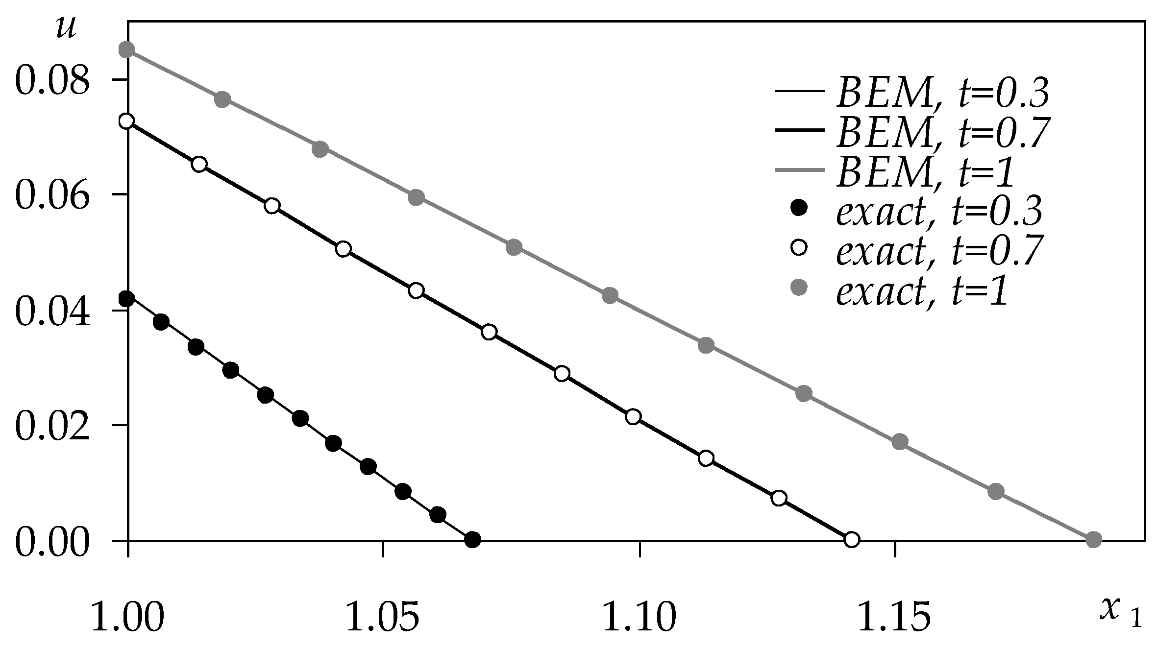
In all the examples with a zero front symmetric relative to the origin, the two-dimensional BEM solutions are also symmetric. Therefore, they are compared with the exact solutions along the axis $O{x}_1$. Figure 1 shows a comparison between the BEM solution and the exact solution in the form of Equation (50) with the following values of the parameters: $\mathsf{\sigma }=3$, $R=1$, $C=5$.

In Example 2, the BEM solution is compared with the exact solution, (48), for the following parameter values: $\mathsf{\lambda }=1$, $\mathsf{\gamma }=3$, $R=1$, $\mathsf{\mu }=1$, $\mathsf{\omega }=0.5$. The comparison is shown in Figure 2.

The calculation results for various values of the parameters agree well with the exact solution, (48). In all the calculation variants, the greatest deviation of the numerical solution from the exact one at different times occurs on the boundary $S^{\left(0\right)}$, and this agrees well with the form of the boundary condition (27). Therefore, the relative error along $S^{\left(0\right)}$ is used to estimate the accuracy of the BEM solution for Example 2.

Table 1. Relative errors of BEM solutions for various numbers of boundary elements.

t	h	Relative Error
		N = 150	N = 250	N = 300	N = 350
0.3	0.1	0.00069	0.00047	0.00039	0.00035
0.6	0.1	0.00081	0.00058	0.00048	0.00043
1	0.1	0.00095	0.00071	0.00060	0.00052
0.3	0.05	0.00061	0.00041	0.00034	0.00029
0.6	0.05	0.00072	0.00051	0.00043	0.00037
1	0.05	0.00084	0.00062	0.00054	0.00045

shows the relative errors of the BEM solutions on the boundary $S^{\left(0\right)}$ for various numbers of the boundary elements for $h=0.1$ and $h=0.05$. The linear functions $f_i=1+r_i$ are used in these calculations as RBFs. The calculations were made for $\mathsf{\epsilon }={10}^{-7}$.

The calculation results demonstrate a high efficiency in solving problems (26) and (27) by the boundary element method, as well as convergence with an increasing number of boundary elements.

6. Analysis of Using Radial Basis Functions

A crucial issue of the effectiveness of the presented algorithm is to select a system of RBFs and their parameters as the most suitable for the class of problems under study. To analyze the use of various kinds of RBF, the constructed algorithm is implemented in the form of a program. The analysis is based on comparing the calculation results for the Example 2, considered in the previous section, with the exact solution in the form of Equation (48).

The form of the RBFs, their shape parameters and the time step are taken as analysis factors. Five RBF systems are considered, namely, the polyharmonic splines $f_i=r_i$ and $f_i=r_i^3$, the linear functions $f_i=1+r_i$, the scaled linear functions $f_i=1+\mathsf{\delta }{r}_i$, and the multiquadric functions $f_i=\sqrt{1+{\left(\mathsf{\delta }{r}_i\right)}^2}$. The analysis is aimed at estimating the effect of the form of the RBF and the value of the shape parameter $\mathsf{\delta }$ on the solution accuracy.

The solutions obtained at different RBFs and parameter values are fairly close. The solution accuracy estimation results are shown in

Table 2. Relative errors of BEM solutions for various RBFs.

t	h	Relative Error
		${\mathit{f}}_{\mathit{i}}={\mathit{r}}_{\mathit{i}}$	${\mathit{f}}_{\mathit{i}}={\mathit{r}}_{\mathit{i}}^3$	${\mathit{f}}_{\mathit{i}}=1+{\mathit{r}}_{\mathit{i}}$	${\mathit{f}}_{\mathit{i}}=1+{\mathbf{\delta }}_1{\mathit{r}}_{\mathit{i}}$	${\mathit{f}}_{\mathit{i}}=1+{\mathbf{\delta }}_2{\mathit{r}}_{\mathit{i}}$	${\mathit{f}}_{\mathit{i}}=\sqrt{1+{\left({\mathbf{\delta }}_1{\mathit{r}}_{\mathit{i}}\right)}^2}$	${\mathit{f}}_{\mathit{i}}=\sqrt{1+{\left({\mathbf{\delta }}_2{\mathit{r}}_{\mathit{i}}\right)}^2}$
0.3	0.1	0.00064	0.00048	0.00035	0.00017	0.00015	0.00012	0.00011
0.6	0.1	0.00077	0.00060	0.00043	0.00020	0.00017	0.00016	0.00014
1	0.1	0.00094	0.00074	0.00052	0.00024	0.00021	0.00022	0.00019
0.3	0.05	0.00058	0.00040	0.00029	0.00016	0.00014	0.00010	0.00010
0.6	0.05	0.00072	0.00054	0.00037	0.00018	0.00015	0.00013	0.00012
1	0.05	0.00087	0.00067	0.00045	0.00023	0.00018	0.00019	0.00016

. The table shows relative errors along the boundary $S^{\left(0\right)}$ at three moments of time for BEM solutions obtained with the use of various RBFs, with the time steps $h=0.1$ and $h=0.05$ when $N=350$. The values ${\mathsf{\delta }}_1=1/\left(0.815d\right)$, where $d=\left(1/N\right){\displaystyle \sum _{i=1}^N{d}_i}$, $d_i$ is the distance from the i-th collocation point to the nearest other point [31], and ${\mathsf{\delta }}_2=0.8\sqrt{N}/D$, where $D$ is the diameter of the smallest circle containing all the collocation points [32], are taken as the values of the shape parameter in the scaled linear functions and in the multiquadrics.

The calculations have shown that the solution accuracy increases as the time step decreases, and this testifies to the convergence of the algorithm developed. The comparison among the results of using different RBF systems enables us to make the following inferences. The BEM solutions obtained with the use of all the selected RBFs have small relative errors, so that the algorithm is stable with respect to the choice of RBFs. The best results have been obtained with the use of the multiquadric functions.

Thus, the developed algorithm, based on BEM with the application of the dual reciprocity method, allows one to solve, with a high accuracy, problems of the form expressed by Equations (26) and (27) in a finite time interval.

7. Conclusions

The paper has discussed the problem of constructing a heat wave for a nonlinear heat conduction equation with a source (sink) in the case of two spatial variables. In order to solve this problem, the following two different approaches are applied: the power series method, enabling one to prove the existence and uniqueness of the solution in the neighborhood of the initial time moment and to construct the solution in the form of a converging power series, and the boundary element method, allowing the problem to be solved on a specified finite time interval. Calculations showing a stable convergence of the algorithm have been made. Exact solutions have been used to verify the numerical method, their construction being reduced to the integration of the Cauchy problem for the second-order ODE with a singularity. The comparison of the BEM calculations with the here-obtained solutions has testified to a practically complete coincidence, which allows the conclusion that the BEM algorithm works correctly.

Further research may involve consideration of other heat wave initiation problems in a two-dimensional statement, as well as an increase in the problem dimensionality.

References

- Vazquez, J.L. The Porous Medium Equation: Mathematical Theory; Clarendon Press: Oxford, UK, 2007. [Google Scholar] [CrossRef]
- Evans, L.C. Partial Differential Equations, 2nd ed.; American Mathematical Society: Providence, RI, USA, 2010. [Google Scholar] [CrossRef] [Green Version]
- Barenblatt, G.I.; Entov, V.M.; Ryzhik, V.M. Theory of Fluid Flowsthrough Natural Rocks; Kluwer Academic Publishers: Dordrecht, The Netherlands; Boston, MA, USA, 1990. [Google Scholar]
- Sidorov, A.F. Analytic representations of solutions of nonlinear parabolic equations of time-dependent filtration (porous medium) type. Sov. Math. Dokl. 1985, 31, 40–44. [Google Scholar]
- Filimonov, M.Y.; Korzunin, L.G.; Sidorov, A.F. Approximate methods for solving nonlinear initial boundary-value problems based on special construction of series. Russ. J. Numer. Anal. Math. Model. 1993, 8, 101–125. [Google Scholar] [CrossRef]
- Sidorov, N.A.; Loginov, B.V.; Sinitsyn, A.V.; Falaleev, M.V. Lyapunov-Schmidt Methods in Nonlinear Analysis and Applications; Kluwer Academic Publishers: Dordrecht, The Netherlands, 2002. [Google Scholar] [CrossRef]
- Sidorov, N.A. Classic Solutions of Boundary Value Problems for Partial Differential Equations with Operator of Finite Index in the Main Part of Equation. Bull. Irkutsk State Univ. Ser. Math. 2019, 27, 55–70. [Google Scholar] [CrossRef]
- Sidorov, D.N.; Sidorov, N.A. Generalized solutions in the problem of dynamical systems modeling by Volterra polynomials. Autom. Remote Control 2011, 72, 1258–1263. [Google Scholar] [CrossRef]
- Wrobel, L.C.; Brebbia, C.A.; Nardini, D. The dual reciprocity boundary element formulation for transient heat conduction. In Finite Elements in Water Resources VI; Springer: Berlin, Germany, 1986; pp. 801–811. [Google Scholar]
- Tanaka, M.; Matsumoto, T.; Yang, Q.F. Time-stepping boundary element method applied to 2-D transient heat conduction problems. Appl. Math. Model. 1994, 18, 569–576. [Google Scholar] [CrossRef]
- Tanaka, M.; Matsumoto, T.; Takakuwa, S. Dual reciprocity BEM for time-stepping approach to the transient heat conduction problem in nonlinear materials. Comput. Methods Appl. Mech. Eng. 2006, 195, 4953–4961. [Google Scholar] [CrossRef]
- Divo, E.; Kassab, A.J. Transient non-linear heat conduction solution by a dual reciprocity boundary element method with an effective posteriori error estimator. Comput. Mater. Contin. 2005, 2, 277–288. [Google Scholar] [CrossRef]
- Wrobel, L.C.; Brebbia, C.A. The dual reciprocity boundary element formulation for nonlinear diffusion problems. Comput. Methods Appl. Mech. Eng. 1987, 65, 147–164. [Google Scholar] [CrossRef]
- Singh, K.M.; Tanaka, M. Dual reciprocity boundary element analysis of transient advection-diffusion. Int. J. Numer. Method H 2003, 13, 633–646. [Google Scholar] [CrossRef]
- AL-Bayati, S.A.; Wrobel, L.C. A novel dual reciprocity boundary element formulation for two-dimensional transient convection–diffusion–reaction problems with variable velocity. Eng. Anal. Bound. Elem. 2018, 94, 60–68. [Google Scholar] [CrossRef]
- Fendoglu, H.; Bozkaya, C.; Tezer-Sezgin, M. DBEM and DRBEM solutions to 2D transient convection-diffusion-reaction type equations. Eng. Anal. Bound. Elem. 2018, 93, 124–134. [Google Scholar] [CrossRef]
- Powell, M.J.D. The Theory of Radial Basis Function Approximation. In Advances in Numerical Analysis; Light, W., Ed.; Oxford Science Publications: Oxford, UK, 1992; Volume 2. [Google Scholar]
- Golberg, M.A.; Chen, C.S.; Bowman, H. Some recent results and proposals for the use of radial basis functions in the BEM. Eng. Anal. Bound. Elem. 1999, 23, 285–296. [Google Scholar] [CrossRef]
- Kazakov, A.L.; Spevak, L.F. Numerical and analytical studies of a nonlinear parabolic equation with boundary conditions of a special form. Appl. Math. Model. 2013, 37, 6918–6928. [Google Scholar] [CrossRef]
- Kazakov, A.L.; Spevak, L.F. An analytical and numerical study of a nonlinear parabolic equation with degeneration for the cases of circular and spherical symmetry. Appl. Math. Model. 2016, 40, 1333–1343. [Google Scholar] [CrossRef]
- Kazakov, A.L.; Lempert, A.A. Existence and uniqueness of the solution of the boundary-value problem for a parabolic equation of unsteady filtration. J. Appl. Mech. Tech. Phys. 2013, 54, 251–258. [Google Scholar] [CrossRef]
- Polyanin, A.D.; Zaitsev, V.F. Handbook of Nonlinear Partial Differential Equations; Chapman and Hall/CRC Press: Boca Raton, FL, USA; London, UK; New York, NY, USA, 2012. [Google Scholar]
- Kosov, A.A.; Semenov, E.I. Exact Solutions of the Nonlinear Diffusion Equation. Sib. Math. J. 2019, 60, 93–107. [Google Scholar] [CrossRef]
- Filimonov, M. Application of method of special series for solution of nonlinear partial differential equations. In AIP Conference Proceedings; American Institute of Physics: College Park, MD, USA, 2014; Volume 1631, p. 218. [Google Scholar] [CrossRef]
- Samarskii, A.A.; Galaktionov, V.A.; Kurdyumov, S.P.; Mikhailov, A.P. Blow-Up in Quasilinear Parabolic Equations; De Gruyte: Berlin, Germany; New York, NY, USA, 1995. [Google Scholar] [CrossRef]
- Kazakov, A.L.; Orlov, S.S.; Orlov, S.S. Construction and study of exact solutions to a nonlinear heat equation. Sib. Math. J. 2018, 59, 427–441. [Google Scholar] [CrossRef]
- Sinelshchikov, D.I.; Kudryashov, N.A. Integrable Nonautonomous Liénard-Type Equations. Theor. Math. Phys. 2018, 196, 1230–1240. [Google Scholar] [CrossRef]
- Guha, P.; Ghose-Choudhury, A. Nonlocal transformations of the generalized Liénard type equations and dissipative Ermakov-Milne-Pinney systems. Int. J. Geom. Methods Mod. Phys. 2019, 16, 1950107. [Google Scholar] [CrossRef] [Green Version]
- Brebbia, C.A.; Telles, J.C.F.; Wrobel, L.C. Boundary Element Techniques; Springer: Berlin, Germany, 1984. [Google Scholar] [CrossRef]
- Fedotov, V.P.; Spevak, L.F. One approach to the derivation of exact integration formulae in the boundary element method. Eng. Anal. Bound. Elem. 2008, 32, 883–888. [Google Scholar] [CrossRef]
- Hardy, R.L. Multiquadric equations of topography and other irregular surfaces. J. Geophys. Res. 1971, 76, 1905–1915. [Google Scholar] [CrossRef]
- Franke, R. Scattered data interpolation: Tests of some methods. Math. Comput. 1982, 38, 181–200. [Google Scholar] [CrossRef]
Figure 1.
Comparison between the BEM solution and the exact solution, .
Figure 2.