Corrected Maximum Likelihood Estimations of the Lognormal Distribution Parameters


Department of Mathematics, Beijing Jiaotong University, Beijing 100044, China
*
Author to whom correspondence should be addressed.
Symmetry 2020, 12(6), 968; https://0-doi-org.brum.beds.ac.uk/10.3390/sym12060968
Submission received: 15 May 2020
/
Revised: 27 May 2020
/
Accepted: 29 May 2020
/
Published: 6 June 2020
Abstract
:As a result of asymmetry in practical problems, the Lognormal distribution is more suitable for data modeling in biological and economic fields than the normal distribution, while biases of maximum likelihood estimators are regular of the order , especially in small samples. It is of necessity to derive logical expressions for the biases of the first-order and nearly consistent estimators by bias correction techniques. Two methods are adopted in this article. One is the Cox-Snell method. The other is the resampling method known as parametric Bootstrap. They can improve maximum likelihood estimators performance and correct biases of the Lognormal distribution parameters. Through Monte Carlo simulations, we obtain average root mean squared error and bias, which are two important indexes to compare the effect of different methods. The numerical results reveal that for small and medium-sized samples, the performance of analytical bias correction estimation is superior than bootstrap estimation and classical maximum likelihood estimation. Finally, an example is given based on the actual data.
1. Introduction
Because of its flexibility and universality, the Lognormal distribution is a commonly used reliability function distribution, which can be applied to describe the fatigue life and wear resistance of products in the article of [1]. And [2] introduces the latest computer statistical method for test plan and reliability data analysis of industrial products. The Lognormal distribution is asymmetrical and positively skewed. The hazard rate function of this distribution always starts at zero, rises to the maximum, and then drops to zero at a slow pace. Hence, when positive studies suggest that the hazard rate of potential distribution is nonmonotone and single-peaked, these factual data can be analyzed by the Lognormal distribution. As shown by [3], in the table associated with normal (Gaussian) random variables, approximate values of the hazard rate that can be used to calculate the parameter values outside of the usual range are presented. At present, [4] is the first one to put forward the Lognormal distribution theory in detail. In the late 1920’s, there was an independent development path in small-particle statistics with the Lognormal distribution. [5] pointed out the applicability of truncated or censored lognormal distributions and [6] applied his theory to biological data which appeared as discrete counts. In this case, [7] further studied the Lognormal distribution.
Most of the existing statistical analysis methods based on the hypothesis of the normal distribution of data. Nevertheless, for data that does not contain negative values or is otherwise distorted, the assumption of normality is not realized—which is common in different disciplines such as biology, politics, philology, economics, physical, finance and sociology. In this case, the Lognormal distribution can better fit the data.
When an event is affected by multiple factors, the distribution of these factors is unknown. According to the central limit theorem, after they are all added up, the average value of the result is concerned as the normal distribution. Because of the existence of the central limit theorem, we use the normal distribution to obtain most theoretical arguments. This theorem shows that with the increase of the number of variables in the normal distribution, the distribution which is standardized random variable summation approaches to unit a normal distribution. Nevertheless, on account of the symmetry of the normal distribution, it can not accurately estimate actual problems. Because many natural growth processes do not add up independently. They are related to each other and driven by the accumulation of many small percentage changes. When inversely transformed to the initial scale, it makes the scale distribution approximate to the Lognormal distribution. They are multiplicative and additive on the logarithmic scale. Refs. [8,9] pointed out that an important difference amid the normal distribution and the Lognormal distribution is that the former is on the basic effect of multiplication and the latter is based on addition. Taking logarithm can make us change multiplication into addition.
If normal distribution is followed by , we believe random variable X follows the Lognormal distribution. In some cases, X only takes positive value. The calculation mean and median can be different. Especially when there is a large value in the data, the arithmetic mean will be seriously affected. Face so of circumstance, the Lognormal distribution is better for data fitting. The geometric mean usually represents median, but arithmetic mean is greater than median, resulting in right deviation of distribution. The curve of the Lognormal distribution is usually right-skewed, with long tail on the right-hand position and narrow array on the left-hand sideways. The Lognormal distribution is similar to Weibull distribution in some shape parameters, and some data suitable for Weibull distribution are also appropriate for Lognormal distribution.
In this paper, we discuss some useful methods which can correct the maximum likelihood estimators from the Lognormal distribution and deduce specific formulae of bias with limited samples. The probability density function of Lognormal distribution is written as:
where , and . The mathematical expectation of the Lognormal distribution is . For a given parameter , when tends to zero, the mathematical expectation tends to .
Then, the function of the failure rate is written as:
where is probability density function of standard normal distribution and is its distribution function.
The failure rate function is applicable to non monotonic data of inverted bathtub shape. When the parameter is small, it can be simplified as the failure rate increasing model. When the parameter is large, it can be simplified as the failure rate decreasing model. And the Lognormal distribution is applied to reliability analysis of semiconductor devices and fatigue life of some kinds of mechanical parts. Its main purpose is to analyze the repair time data accurately in the maintainability analysis.
The Lognormal distribution has many important applications in financial asset prices such as Black-Scholes equations and in reliability engineering in [10]. The Lognormal distribution is also widely applied to the realms of health care. For example, Ref. [11] pointed out that the transcriptional level of different genes is consistent with the Lognormal distribution and provided a more exact method to estimate the gene activity of the typical cell. Ref. [12] exploited the age distribution of Perthes disease is log-normal.
For the curve with horizontal asymptote, the standard concept of additive homogeneous error of symmetrical distribution will appear almost inevitably. When estimating parameters of any probability distribution, it is very important to choose the estimation method. No matter for real data or random simulation data, the most commonly used approach in all classical estimation techniques is maximum likelihood estimation. Under normal regularity circumstances, it is invariant, asymptotically consistent, as well as asymptotically normal. Therefore, we mainly observe the maximum likelihood estimators for Lognormal distribution parameters. However, we observe that these excellent properties can only be realized in large-sample size. In the limited samples, especially in the small samples, the maximum likelihood estimation (MLE) is often biased. Since the characteristic of likelihood equation of the Lognormal distribution is usually highly non-linear and it also have an unclosed form solution, it can be complex to determine such bias. In realistic application, in order to increase the accuracy in estimation, it is very essential to obtain the closed expression of the first-order deviation of the estimator. Many researchers have corrected the bias of different distributions. Readers can refer to [13,14,15,16,17,18,19,20,21].
We focus on two approaches to modify the bias of MLEs from the first order to the second order, and illustrate their effects. Ref. [22] recommended a method to obtain specific bias analytical expressions. Then we use these expressions to develop the bias of MLEs, and get the consistent second order. Instead of the analytically bias-adjusted MLEs, Ref. [23] introduced the parametric Bootstrap resampling method. The two methods are compared with the classical MLE in terms of error reduction and root mean square error. On the basis of results, a conclusion is drawn that the analytic method is suitable for the Lognormal distribution.
In the article remaining part is arranged as follows. A brief Section 2 describes the parametric point estimation for the Lognormal distribution by maximum likelihood method. In Section 3, we describe the Cox-Snell bias-corrected method and parametric bootstrap resampling method. And these methods are used in the Lognormal distribution. Section 4, contains simulation by Monte Carlo as used to contrast action of Cox-Snell bias adjustment estimation, bootstrap bias adjustment estimation and MLE. In Section 5, for the purpose of illustrating the point, the application of real data are proposed. Eventually, the summary of the article is in Section 6.
2. Maximum Likelihood Estimator
Lognormal distribution maximum likelihood estimators are discussed in this part. If are randomly selected from independent observations which obey the Lognormal distribution. From (1), the function of the likelihood can be donated as below:
where and are two unknown parameters, and , .
The function of log-likelihood of and is denoted as below:
The MLEs of and are and which can be solved from the following equations:
The expected information matrix is defined as:
The inverse of K is expressed as:
3. Bias-Corrected MLEs
We adopt the method proposed by [22] and the parametric Bootstrap resampling method (Efron 1982). Both methods modify maximum likelihood estimators by reducing the bias order.
3.1. Cox-Snell Methodology
According to observation samples of size n and r-dimensional parameter vector , we can derive . Due to properties of logarithm and derivative, the likelihood function is always regular for all derivatives even the third derivative. The derivatives joint cumulant is expressed as:
where the function of the log-likelihood is , .
Moreover, the derivatives of can be written as:
All of the derivatives joint cumulants are presumed to be . The data of the corresponding sample are independent but not strictly subject to the same distribution. The element bias of the can be denoted as follows:
where . element of the inverse expected information matrix is . Furthermore, in the case of non independent and every term of the k is , the bias equation is also applicable, It can be adjusted as:
In terms of calculation, we normally choose this expression to evaluate, because it does not relate to terms of . Define , where , and the matrix of A is obtained as:
The bias of can be re-expressed in the concise form:
The bias correction of can be given by:
It is noteworthy that from (9), the expected value of joint cumulants results of derivatives can be calculated. For this reason this methodology is suitable for the Lognormal distribution. If the analytical solution cannot be obtained, the numerical solution can be used instead.
Next, we ought to calculate the third derivative of the two parameters of the Lognormal distribution. From (7) and (8), it follows that:
Due to the higher-order derivatives and observations x, we can obtain the derivatives of cumulants. From and , we have:
The information matrix is
Thus, in the process of MLE, the bias which is to order of the estimated values of and are expressed, separately, as:
Bias-adjusted estimators are then given by:
We observe the bias-corrected estimation (BCE) of is 0. According to the behavior of the Lognormal distribution, we consider that it is related to the linear property of maximum likelihood estimation of parameter . It is to be noted that is consistent to order .
3.2. Parametric Bootstrap
Bootstrap method can be divided into parametric method and nonparametric method. When the distribution of original data is clear, it is generally considered that the efficiency of parametric method is higher than that of nonparametric method. According to the characteristics of this paper, we decided to adopt the parameter bootstrap method.
Bootstrap theory is applied to assess the bias of maximum likelihood estimate, carried out in a parametric framework. Efron introduced the parametric Bootstrap resampling estimation (PBE) in 1982. Suppose random variable X is from distribution function F. Then we randomly select n samples from X. And is a parameter related to function F. The estimator of is . In order to resample, we generate a great quantity pseudo samples , and calculate respectively. In such a scenario, the factual values generate of parameters are MLEs of the and is the data for the second MLEs. Then, the empirical distribution of can be applied to assess the distribution function of . If is a finite dimensional parameter family of F, according to the consistency of the distribution, the parameter estimation of F can be obtained by using a estimator . The bias of the is expressed as:
where is the expectation of F distribution. By substituting for F, we can get the bias of parametric bootstrap estimation.
Based on the original samples, we generate independent bootstrap samples of size B and calculate the bootstrap estimators for each time as follows . When B is large enough, the expected value is approximately equal to .
The bias-corrected estimators are written as:
where is the MLE of , is the Bootstrap sample. And then the maximum likelihood estimators are regarded as the true values. Therefore, the estimated value from PBE is defined as:
Ref. [24] pointed out that since the estimator is approximate to a constant, it should be called constant bias correction MLE. Compared with BCE, the form of PCE is more convenient and it does not involve the joint cumulants of the derivatives, when this methodology realizes a consistent estimator to second order. However, there is a certain randomness in the process of resampling. This may lead to the risk of unstable correction results.
4. Simulation Results
Based on different sample sizes and the true value of parameters, the effect of the maximum likelihood estimation, analytic correction method and parametric Bootstrap resampling method are compared in a Monte Carlo experiment. root mean squared errors (RMSEs) and average biases are criteria for the assessment. In the process of research, we notice that the characteristics of the Inverse Gaussian distribution are similar to those of the Lognormal distribution. After calculation, we observe that the bias of maximum likelihood algorithm of from the Inverse Gaussian distribution is also equal to zero. Therefore, we evaluate from three approaches in the Inverse Gaussian distribution as well.
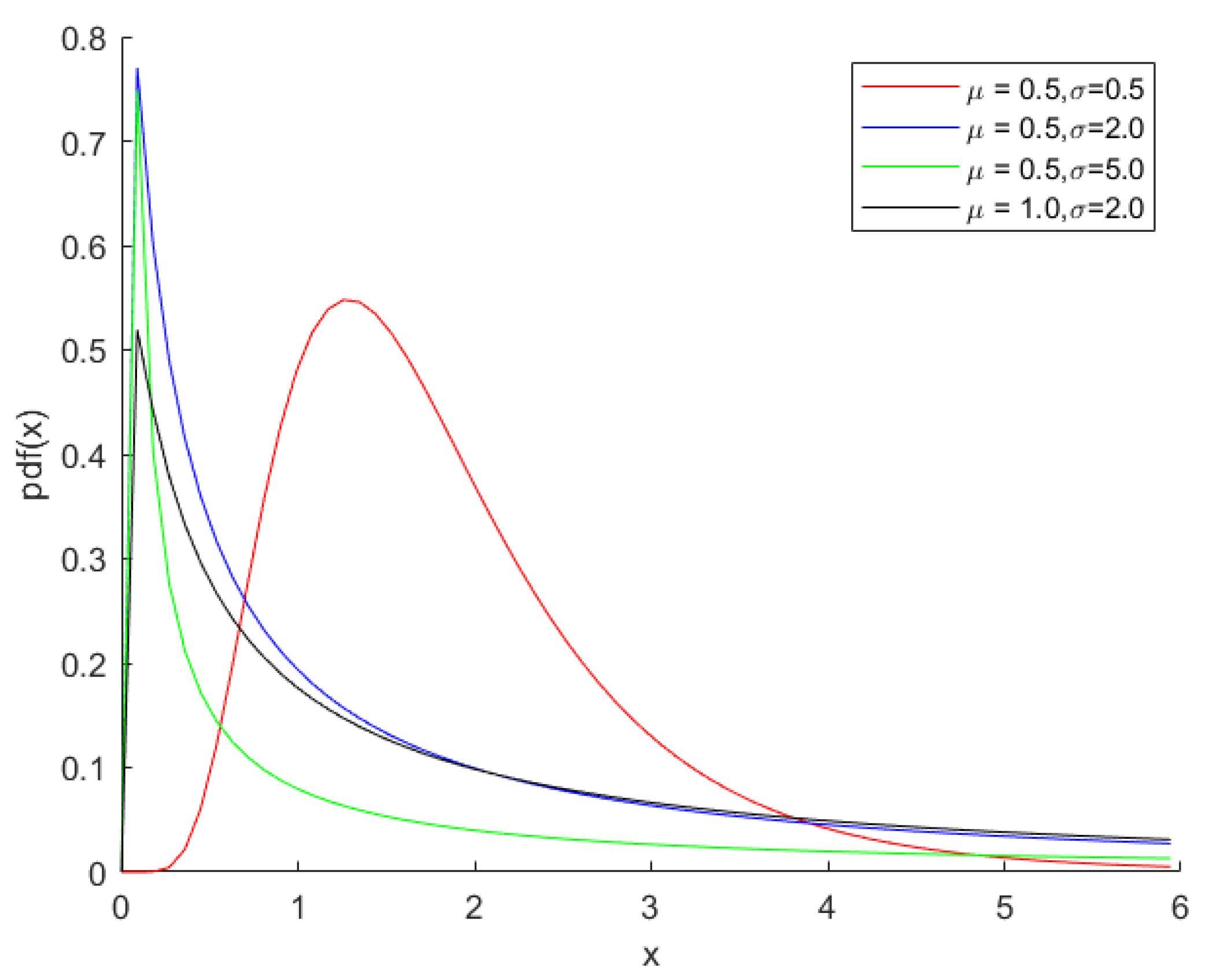
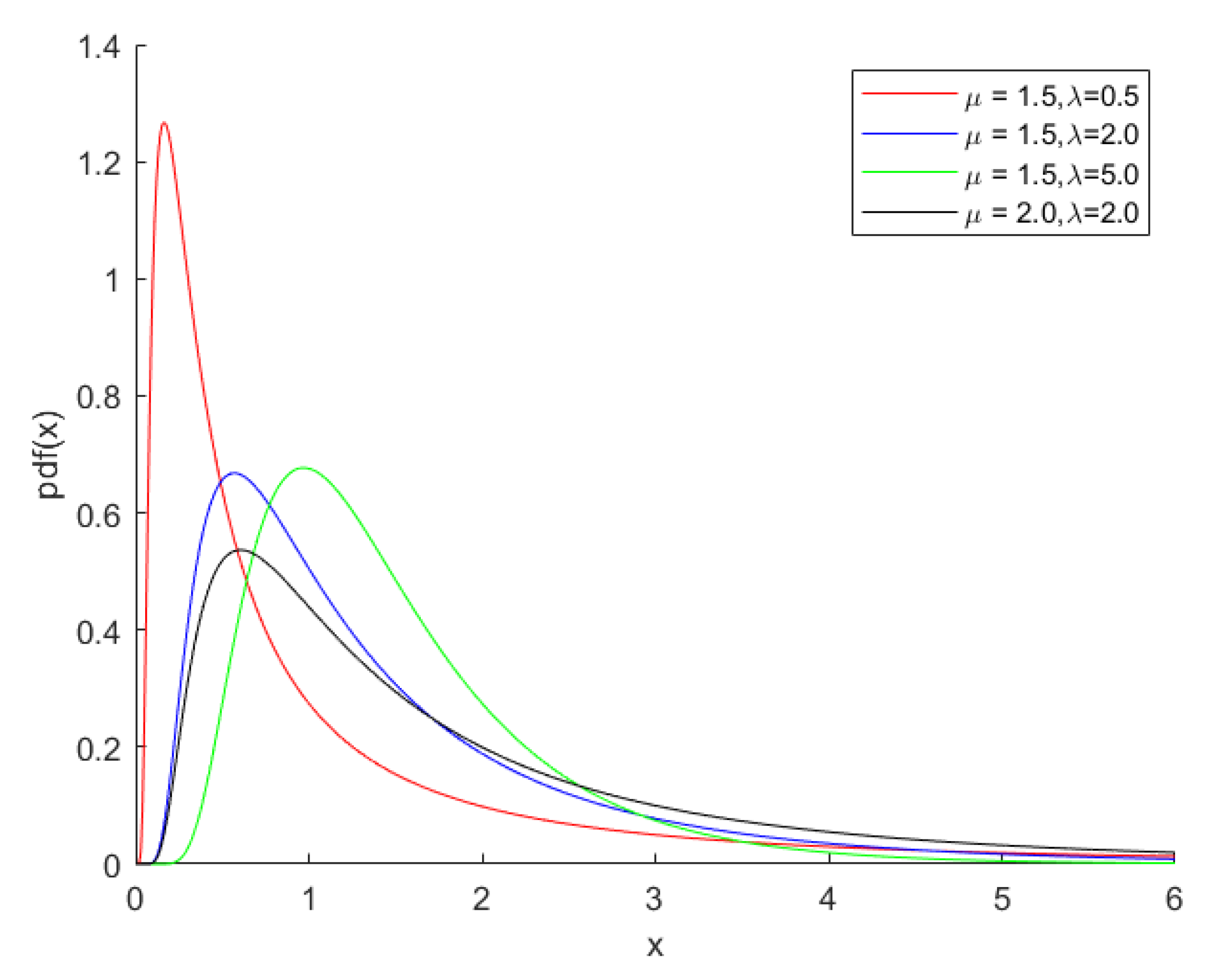
By considering the density curve shown in Figure 1 and Figure 2, different parameter values in the Lognormal distribution and Inverse Gaussian distribution can be selected. We have considered sample sizes of 10, 20, 30, 40, 50 and = 0.5, 1, 1.5, 2 and , = 0.5, 1, 1.5, 2, 3, 5. Using inverse transformation method, pseudo-random samples are generated. Nevertheless, the Lognormal distribution does not have the form of cumulative distribution function(c.d.f). So we generate random numbers of the normal distribution and then take their index.
We use Monte Carlo method for 10,000 repetitions, and use 5000 re-samples to construct bootstrap bias correction. The first two tables are from the Lognormal distribution, and the data of the last two tables are simulated by the Inverse Gaussian distribution.
For results discussion of above methods, we consider the theoretical bias, defined as shown:
In the process of Monte Carlo simulation, we need to bring specific values into the formula. The average bias and RMSE of , and of the sample are defined as
where M is the number of simulations. In this paper, M equals 10,000. If scholars need relevant codes, they can send an email to [email protected].
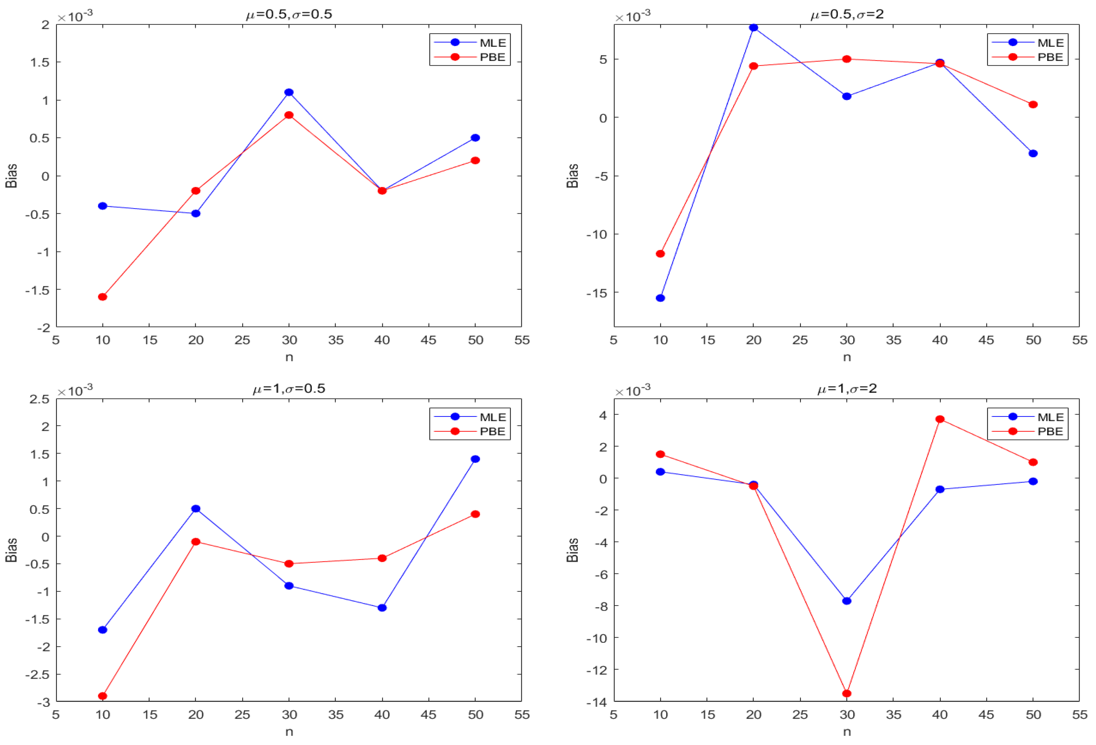
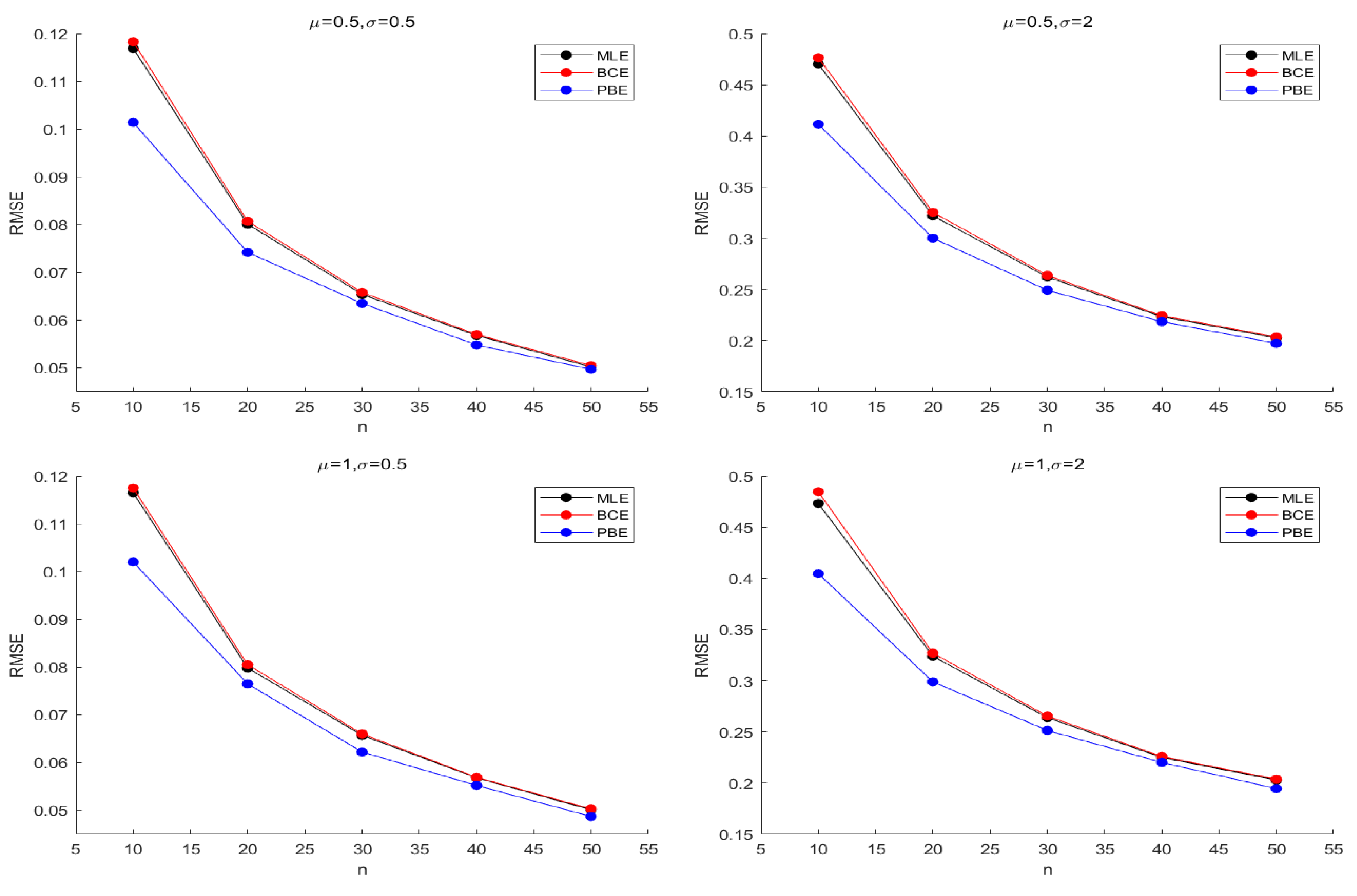
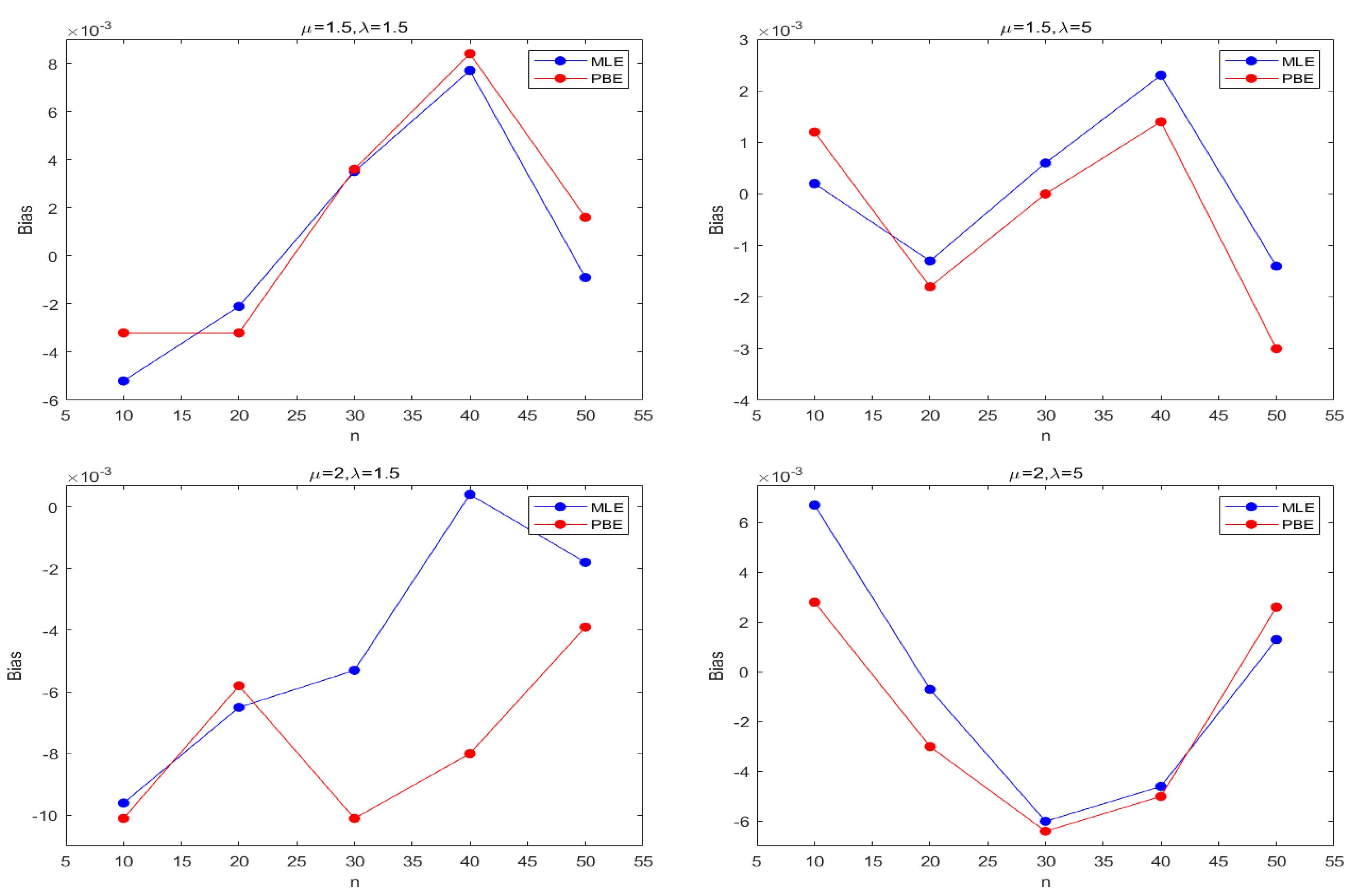
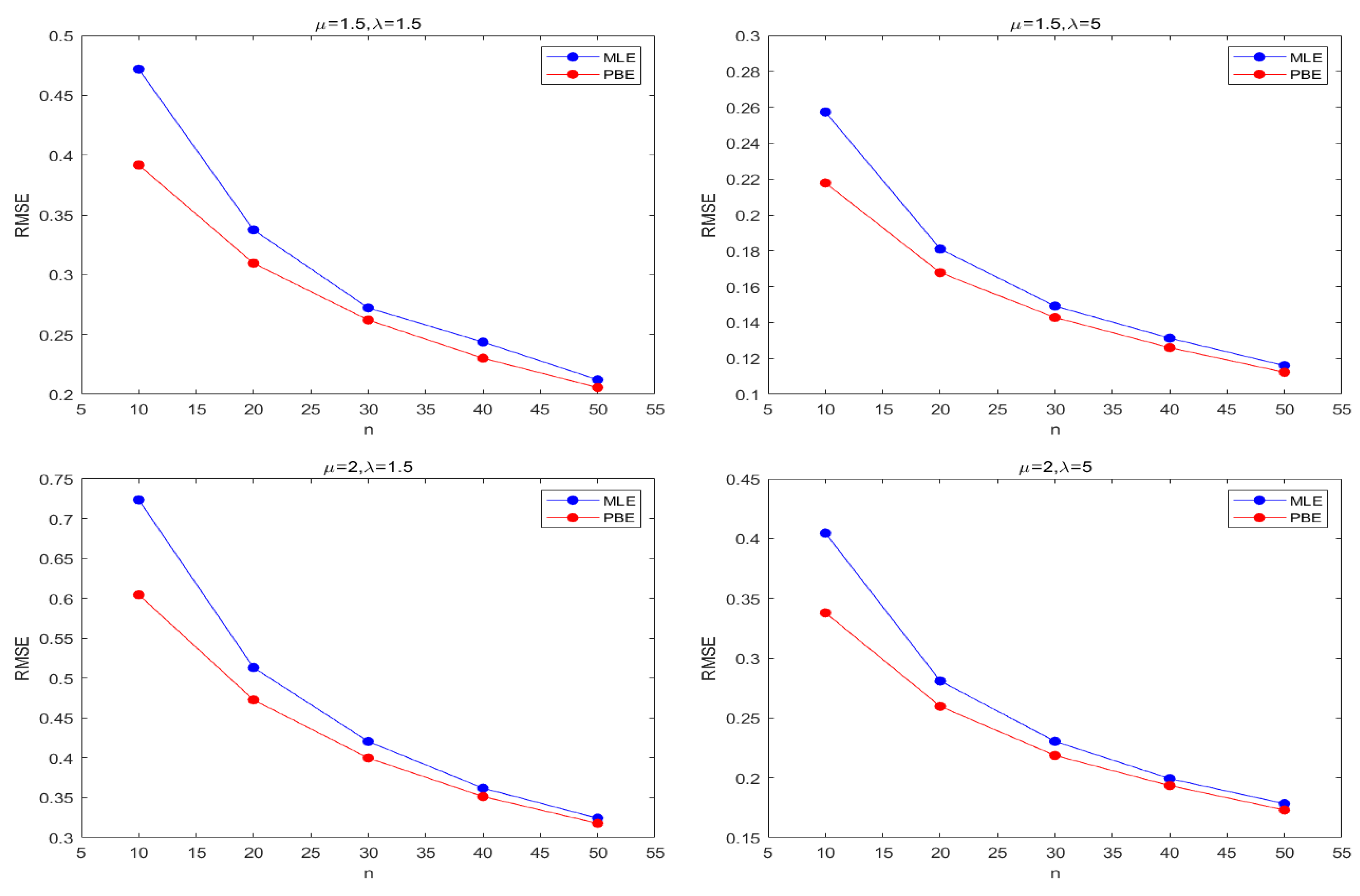
Figure 3 and Figure 4 describe the average and biases of simulated data from the sample size of the Lognormal distribution, and Figure 5 and Figure 6 suggest RMSEs of and from the Lognormal distribution, separately. Based on simulation data, Figure 7 and Figure 8 depict the bias from the Inverse Gaussian distribution. Figure 9 and Figure 10 show RMSEs from Inverse Gaussian distribution.
From Table 1 and Table 2, we can observe that the bias of is much smaller than that of , so it is reasonable that Cox-Snell methodology can only reduce the bias of estimator . Therefore, we mainly consider the bias correction of . The bias of and is always smaller than that of ; the bias of is usually smaller than that of . In general, with the increasing of sample sizes n, the bias of all estimators of is close to zero.
Table 3 and Table 4 show the corresponding results of the Inverse Gaussian distribution. These results and those of the Lognormal distribution have similarities, besides that the performance of analytic bais correction is better. Although the bias of of Inverse Gaussian distribution is larger than that of lognormal distribution, the bias of of Inverse Gaussian distribution is smaller than that of the Lognormal distribution.
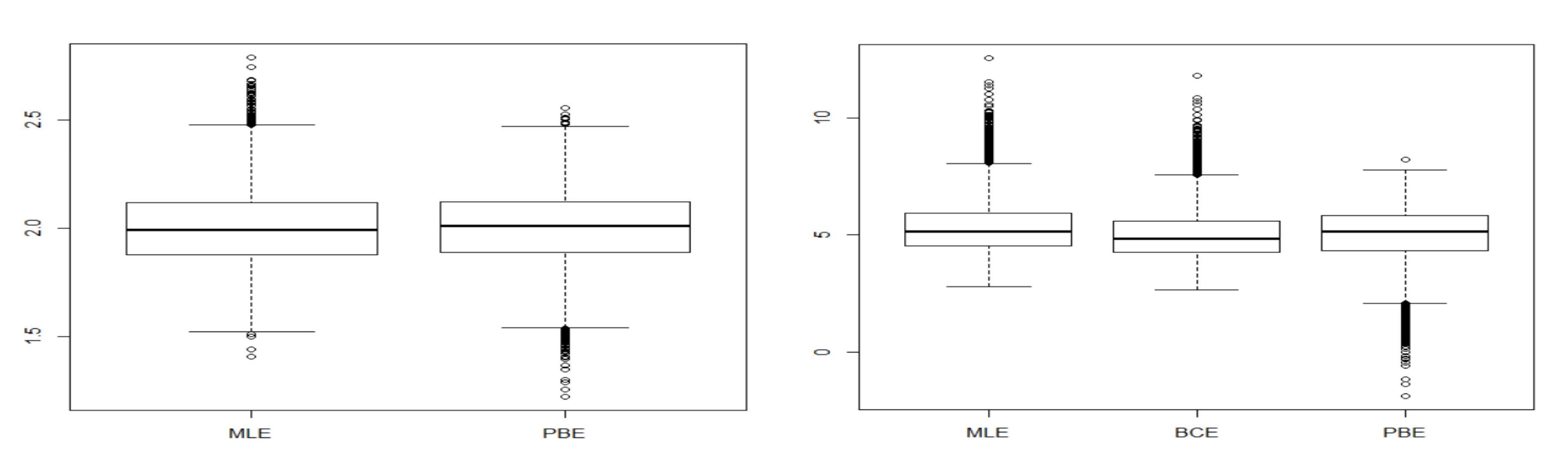
We also show the Lognormal distribution and the Inverse Gaussian distribution parameters estimation when the size is 50 by using the boxplots. Boxplots can convey more information than tables. Figure 11 and Figure 12 show that the parameter estimators are closer to the real values through the bias corrected method. At the same time, Cox Snell method can reduce the range of parameter estimates to a certain extent.
We change parameter values and carry out repeated experiments. It is observed that the result will not change with the change of parameter setting, which shows that Cox-Snell method is robust. In the process of bias correction, the focus of calculation is to find Fisher information matrix. For most distribution functions, this is easy to calculate. In terms of the usability of existing software, we mainly use optim package in R language. This package is efficient and concise, and is suitable for practical calculation.
On this basis, in almost all cases considered, the analytical Cox-Snell method is superior to the bootstrap method and the classical maximum likelihood algorithm. BCE and PBE also reduce the RMSE in the Inverse Gaussian distribution. Therefore, when the standards to measure the correction effect are consistent, it can be determined that the improved estimator is nearer to the real value of parameter than the uncorrected estimator. Maximum likelihood estimators of in the Lognormal distribution and the Inverse Gaussian distribution are unbiased and efficient. In the process of analysis, we find that consistent estimation of is general, when and equal to zero in the expected information matrix. In this case, we can obtain that the bias of maximum likelihood estimator is zero by using Cox and Snell method.
5. Example Illustration
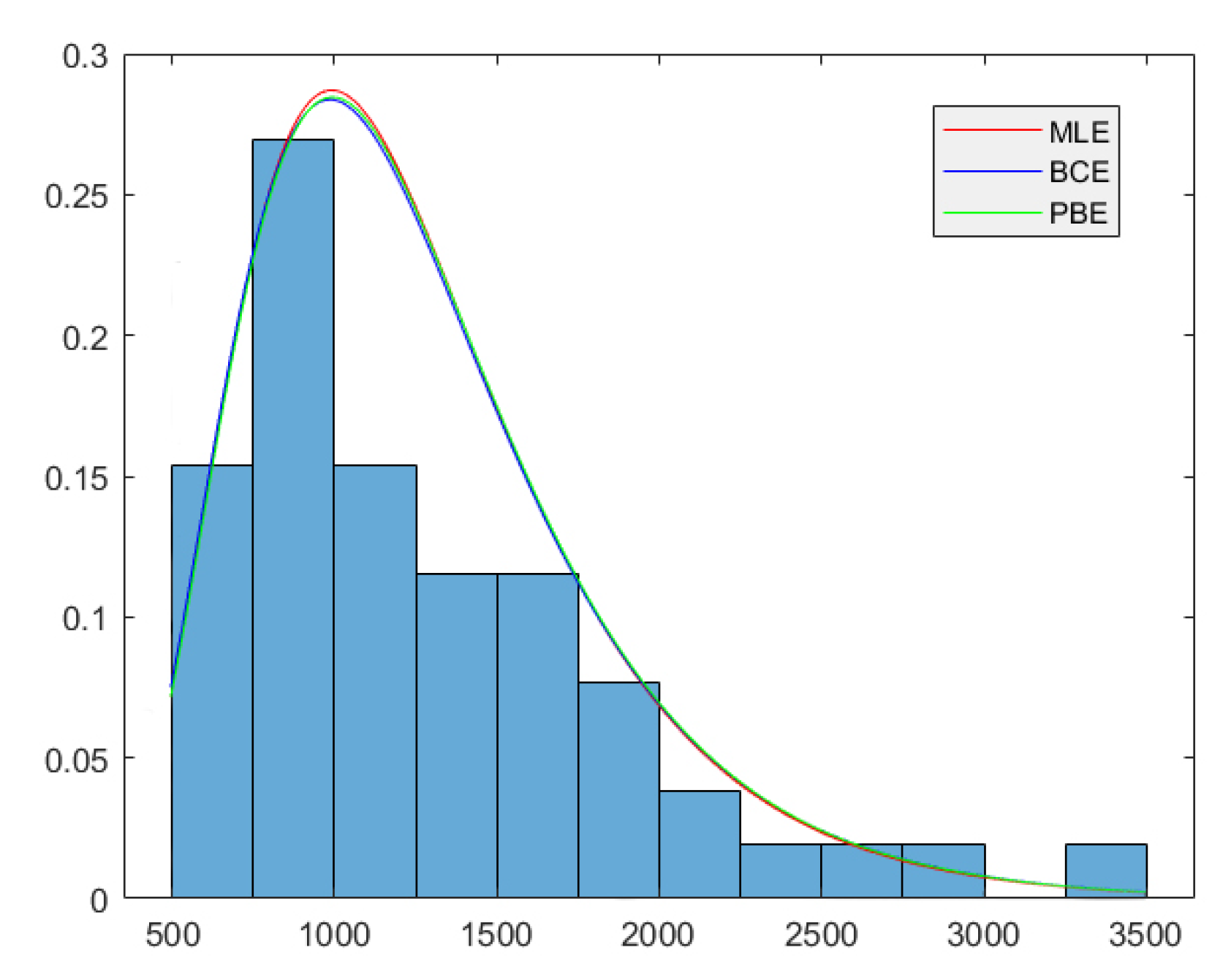
In this part, we use a few actual data to verify whether we can obtain estimators with smaller biases by adopting the Cox-Snell approach and the parameter bootstrap resampling method. The experimental data comes from the daily trading volume of Shanghai stock market in 2002. Data sourced from China Securities Regulatory Commission. We first adopt the maximum likelihood estimation to fit the actual data, and then use the analytic method. Since the estimator of has little difference in various methods, we mainly focus on the correction effect of estimation. Figure 13 depicts the fitting of the Lognormal probability density at different estimators of and . Table 5 shows that for , the lowest RMSE is given by the biased MLE whereas PBE gives the highest RMSE. We also observe that BCE of is the largest and MLE of is the smallest, which is in accordance with the simulation results. Therefore, we have additional evidence that the behavior of the bias correction estimation is superior. It is worth noting that there are obvious differences in the estimators of , which illustrate that in the case of small sample size, bias correction is still necessary due to the effective information contained in the correction method.
To evaluate the degree of figures fitting the Lognormal distribution, we use Kolmogorov-Smirnov (KS) test to calculate D-values and p-values with different parameter values. It is observed that p-values of KS in analytic bias-corrected method derive higher values than MLEs and parametric Bootstrap bias correction and D-values are the opposite. So we have every reason to believe that analytical bias correction can get extremely useful results.
6. Conclusions
The Lognormal distribution and Inverse Gaussian distribution are applied in a broad variety of fields. In practice, the maximum likelihood method is the most used method for these distributions. In this article, we employ the bias-adjusted method recommended by Cox and Snell to increase the accuracy of MLE. We obtain concrete analytical expressions of for the biases and then use these data to construct the biases of the prospective estimated values which are of . Additionally, we have compared a different bias-corrected approach based on Bootstrap resampling. According to the simulation results, we consider that the of two distributions is close to the true value through classical MLEs. When we focus on the other parameter, it is noted that Bootstrap resampling bias correction is not as efficient as Cox-Snell modification in aspect of average bias as well as error of root mean squared, especially in the Inverse Gaussian distribution. In particular, when the sample size increases and the parameter value decreases, the correction effect is better. The bias correction proposed by Cox and Snell is heartily recommended in estimating the Lognormal distribution parameters and the Inverse Gaussian distribution, which is often met in the context of reliability analysis.
In the future work, wild bootstrap is worth considering. In this method, the random weight is generated independent of the model bias and multiplied by the residual to simulate the actual bias distribution. It is suitable for regression analysis the model with heteroskedasticity. In practical analysis, it is characterized by weighted residuals rather than data pairs. Now in the bivariate setting of unknown , it is not a priori clear how to combine coordinate-wise accuracy measures for the two components, but depending on this choice different bias weights result optimal and will lead to different rankings of procedures. And the normal distribution is closely related to the lognormal distribution, so the bias corrected method is also suitable for the normal distribution. As we know, that the MLE is asymptotic, but there is no specific research to prove that Cox-Snell method is also asymptotic. We think it’s worth thinking about in the future work. Then, the Phase-Type distributions are widely used, including many commonly used distributions, such as Erlang, Hypo-empirical and Coxian distributions. Readers can refer to [25]. This distribution can correct some inaccuracies of Weibull distribution in terms of physics. The Phase-Type distributions are non-negative type distributions and have two unknown parameters, which are worth studying in the future work.
Author Contributions
Investigation, S.W.; Supervision, W.G. All authors have read and agreed to the published version of the manuscript.
Funding
This research was supported by Project 202010004009 which was supported by National Training Program of Innovation and Entrepreneurship for Undergraduates.
Acknowledgments
The authors would like to thank the editor and anonymous referees for their constructive comments and suggestions that have substantially improved the original manuscript.
Conflicts of Interest
The authors declare no conflict of interest.
References
- Pinto, J.; Pujol, J.; Cimini, C., Jr. Probabilistic cumulative damage model to estimate fatigue life. Fatigue Fract. Eng. Mater. Struct. 2014, 37, 85–94. [Google Scholar] [CrossRef]
- Meeker, W.Q.; Escobar, L.A. Statistical Methods for Reliability Data; John Wiley & Sons: Hoboken, NJ, USA, 2014. [Google Scholar]
- Sweet, A.L. On the hazard rate of the lognormal distribution. IEEE Trans. Reliab. 1990, 39, 325–328. [Google Scholar] [CrossRef]
- McAlister, D. XIII. The law of the geometric mean. Proc. R. Soc. Lond. 1879, 29, 367–376. [Google Scholar]
- Spiller, D. Truncated log-normal and root-normal frequency distributions of insect populations. Nature 1948, 162, 530–531. [Google Scholar] [CrossRef]
- Thompson, H. Truncated lognormal distributions: I. solution by moments. Biometrika 1951, 38, 414–422. [Google Scholar] [CrossRef]
- Krumbein, W.C. Applications of statistical methods to sedimentary rocks. J. Am. Stat. Assoc. 1954, 49, 51–66. [Google Scholar] [CrossRef]
- Diwakar, R. An evaluation of normal versus lognormal distribution in data description and empirical analysis. Pract. Assess. Res. Eval. 2017, 22, 13. [Google Scholar]
- Limpert, E.; Stahel, W.A. Problems with using the normal distribution–and ways to improve quality and efficiency of data analysis. PLoS ONE 2011, 6, e21403. [Google Scholar] [CrossRef] [Green Version]
- Bishop, P.G.; Bloomfield, R.E. Using a log-normal failure rate distribution for worst case bound reliability prediction. In Proceedings of the 14th International Symposium on Software Reliability Engineering, Denver, CO, USA, 17–20 November 2003; pp. 237–245. [Google Scholar]
- Bengtsson, M.; Ståhlberg, A.; Rorsman, P.; Kubista, M. Gene expression profiling in single cells from the pancreatic islets of langerhans reveals lognormal distribution of mrna levels. Genome Res. 2005, 15, 1388–1392. [Google Scholar] [CrossRef] [Green Version]
- Perry, D.; Skellorn, P.; Bruce, C. The lognormal age of onset distribution in perthes’ disease: An analysis from a large well-defined cohort. Bone Jt. J. 2016, 98, 710–714. [Google Scholar] [CrossRef]
- Saha, K.; Paul, S. Bias-corrected maximum likelihood estimator of the negative binomial dispersion parameter. Biometrics 2005, 61, 179–185. [Google Scholar] [CrossRef] [PubMed]
- Giles, D.E. Bias reduction for the maximum likelihood estimators of the parameters in the half-logistic distribution. Commun. Stat. Theory Methods 2012, 41, 212–222. [Google Scholar] [CrossRef]
- Zaka, A.; Akhter, A.S. Modified moment, maximum likelihood and percentile estimators for the parameters of the power function distribution. Pak. J. Stat. Oper. Res. 2014, 10, 369–388. [Google Scholar] [CrossRef]
- Ling, X.; Giles, D.E. Bias reduction for the maximum likelihood estimator of the parameters of the generalized rayleigh family of distributions. Commun. Stat. Theory Methods 2014, 43, 1778–1792. [Google Scholar] [CrossRef] [Green Version]
- Giles, D.E.; Feng, H.; Godwin, R.T. Bias-corrected maximum likelihood estimation of the parameters of the generalized pareto distribution. Commun. Stat. Theory Methods 2016, 45, 2465–2483. [Google Scholar] [CrossRef]
- Wang, M.; Wang, W. Bias-corrected maximum likelihood estimation of the parameters of the weighted lindley distribution. Commun. Stat. Simul. Comput. 2017, 46, 530–545. [Google Scholar] [CrossRef] [Green Version]
- Mazucheli, J.; Menezes, A.F.B.; Dey, S. Improved maximum-likelihood estimators for the parameters of the unit-gamma distribution. Commun. Stat. Theory Methods 2018, 47, 3767–3778. [Google Scholar] [CrossRef]
- Reath, J.; Dong, J.; Wang, M. Improved parameter estimation of the log-logistic distribution with applications. Comput. Stat. 2018, 33, 339–356. [Google Scholar] [CrossRef] [Green Version]
- Mazucheli, J.; Menezes, A.F.B.; Dey, S. Bias-corrected maximum likelihood estimators of the parameters of the inverse weibull distribution. Commun. Stat. Simul. Comput. 2019, 48, 2046–2055. [Google Scholar] [CrossRef]
- Cox, D.R.; Snell, E.J. A general definition of residuals. J. R. Stat. Soc. Ser. B Methodol. 1968, 30, 248–265. [Google Scholar] [CrossRef]
- Efron, B. The Jackknife, the Bootstrap, and Other Resampling Plans; Siam: Philadelphia, PA, USA, 1982; Volume 38. [Google Scholar]
- MacKinnon, J.G.; Smith, A.A., Jr. Approximate bias correction in econometrics. J. Econ. 1998, 85, 205–230. [Google Scholar] [CrossRef] [Green Version]
- Acal, C.; Ruizcastro, J.E.; Aguilera, A.M.; Jimenezmolinos, F.; Roldan, J.B. Phase-type distributions for studying variability in resistive memories. J. Comput. Appl. Math. 2019, 345, 23–32. [Google Scholar] [CrossRef]
Figure 1.
The Lognormal probability density curve with various values of and .

Figure 2.
The Inverse Gaussian probability density curve with various values of and .

Figure 3.
The bias of average with the Lognormal distribution.

Figure 4.
The bias of average with the Lognormal distribution.

Figure 5.
RMSE of with the Lognormal distribution.

Figure 6.
RMSE of with the Lognormal distribution.

Figure 7.
Average bias of with the Inverse Gaussian distribution.

Figure 8.
Average bias of with the Inverse Gaussian distribution.

Figure 9.
RMSE of with the Inverse Gaussian distribution.

Figure 10.
RMSE of with the Inverse Gaussian distribution.

Figure 11.
Parameter estimations of the Lognormal distribution with , .

Figure 12.
Parameter estimations of the Inverse Gaussian distribution with , .

Figure 13.
Estimated fitted density functions of the daily trading volume in Shanghai.


Table 1.
Relative bias of the Lognormal Distribution ( = 0.5).
| Estimated Values of | Estimated Values of | |||||
|---|---|---|---|---|---|---|
| n | MLE | PBE | MLE | BCE | PBE | |
| 0.5 | 10 | −0.0004 (0.1565) | −0.0016 (0.1457) | −0.0397 (0.1169) | −0.0052 (0.1183) | −0.0054 (0.1014) |
| 20 | −0.0005 (0.1111) | −0.0002 (0.1037) | −0.0192 (0.0801) | −0.0012 (0.0807) | −0.0014 (0.0742) | |
| 30 | 0.0011 (0.0907) | 0.0008 (0.0892) | −0.0123 (0.0654) | −0.0001 (0.0658) | −0.0003 (0.0635) | |
| 40 | −0.0002 (0.0783) | −0.0002 (0.0771) | −0.0097 (0.0568) | −0.0005 (0.0570) | −0.0011 (0.0548) | |
| 50 | 0.0005 (0.0698) | 0.0002 (0.0696) | −0.0070 (0.0502) | 0.0004 (0.0505) | 0.0012 (0.0497) | |
| 100 | 0.0005 (0.0497) | 0.0001 (0.0495) | −0.0039 (0.0353) | −0.0001 (0.0353) | −0.0002 (0.0352) | |
| 200 | −0.0002 (0.0352) | −0.0003 (0.0356) | −0.0018 (0.0249) | 0.0001 (0.0249) | 0.0000 (0.0248) | |
| 1 | 10 | −0.0027 (0.3156) | −0.0025 (0.2897) | −0.0788 (0.2353) | −0.0097 (0.2386) | −0.0103 (0.2031) |
| 20 | −0.0003 (0.2224) | −0.0016 (0.2115) | −0.0380 (0.1601) | −0.0020 (0.1614) | −0.0021 (0.1519) | |
| 30 | 0.0022 (0.1836) | 0.0047 (0.1788) | −0.0245 (0.1316) | −0.0001 (0.1325) | −0.0017 (0.1272) | |
| 40 | 0.0019 (0.1571) | 0.0018 (0.1552) | −0.0180 (0.1133) | 0.0004 (0.1140) | 0.0014 (0.1100) | |
| 50 | −0.0006 (0.1411) | −0.0011 (0.1385) | −0.0160 (0.1000) | −0.0012 (0.1002) | −0.0025 (0.0973) | |
| 100 | 0.0010 (0.1003) | 0.0016 (0.0988) | −0.0076 (0.0703) | −0.0001 (0.0704) | 0.0007 (0.0696) | |
| 200 | 0.0003 (0.0702) | 0.0017 (0.0710) | −0.0039 (0.0503) | −0.0002 (0.0504) | 0.0001 (0.0495) | |
| 1.5 | 10 | 0.0063 (0.4731) | 0.0026 (0.4361) | −0.1215 (0.3481) | −0.0181 (0.3511) | −0.0185 (0.3066) |
| 20 | 0.0007 (0.3313) | 0.0001 (0.3202) | −0.0538 (0.2401) | 0.0005 (0.2428) | 0.0028 (0.2287) | |
| 30 | −0.0006 (0.2729) | −0.0007 (0.2720) | −0.0403 (0.1982) | −0.0038 (0.1990) | −0.0390 (0.1964) | |
| 40 | 0.0027 (0.2415) | 0.0054 (0.2371) | −0.0285 (0.1688) | −0.0009 (0.1695) | −0.0040 (0.1637) | |
| 50 | 0.0026 (0.2137) | 0.0026 (0.2093) | −0.0226 (0.1509) | −0.0005 (0.1514) | 0.0010 (0.1470) | |
| 100 | 0.0001 (0.1538) | −0.0018 (0.1499) | −0.0106 (0.1069) | 0.0006 (0.1072) | 0.0014 (0.1054 ) | |
| 200 | −0.0005 (0.1070) | −0.0017 (0.1054) | −0.0063 (0.0744) | −0.0007 (0.0744) | −0.0014 (0.0741) | |
| 2 | 10 | −0.0155 (0.6346) | −0.0117 (0.5812) | −0.1585 (0.4703) | −0.0204 (0.4764) | −0.0158 (0.4114) |
| 20 | 0.0077 (0.4493) | 0.0044 (0.4325) | −0.0729 (0.3219) | −0.0006 (0.3253) | 0.0019 (0.3001) | |
| 30 | 0.0018 (0.3654) | 0.0050 (0.3519) | −0.0499 (0.2622) | −0.0011 (0.2638) | −0.0026 (0.2492) | |
| 40 | 0.0047 (0.3141) | 0.0046 (0.3111) | −0.0377 (0.2234) | −0.0009 (0.2244) | −0.0009 (0.2185) | |
| 50 | −0.0031 (0.2796) | 0.0011 (0.2782) | −0.0293 (0.2027) | 0.0003 (0.2036) | −0.0011 (0.1973) | |
| 100 | 0.0009 (0.1984) | 0.0041 (0.1988) | −0.0170 (0.1429) | −0.0022 (0.1429) | −0.0022 (0.1419) | |
| 200 | −0.0024 (0.1395) | 0.0006 (0.1409) | −0.0072 (0.1013) | 0.0002 (0.1014) | 0.0009 (0.1003) | |
| 3 | 10 | −0.0178 (0.9540) | −0.0042 (0.8750) | −0.2406 (0.7005) | −0.0337 (0.7080) | −0.0325 (0.6084) |
| 20 | −0.0111 (0.6683) | −0.0117 (0.6280) | −0.1138 (0.4822) | −0.0056 (0.4862) | −0.0147 (0.4408) | |
| 30 | −0.0076 (0.5479) | −0.0088 (0.5337) | −0.0782 (0.4014) | −0.0051 (0.4036) | −0.0053 (0.3756) | |
| 40 | −0.0054 (0.4764) | −0.0039 (0.4663) | −0.0540 (0.3341) | 0.0013 (0.3359) | 0.0046 (0.3292) | |
| 50 | 0.0032 (0.4253) | 0.0049 (0.4185) | −0.0449 (0.3033) | −0.0006 (0.3045) | 0.0044 (0.2958) | |
| 100 | −0.0015 (0.3014) | 0.0004 (0.2988) | −0.0226 (0.2135) | −0.0003 (0.2139) | −0.0020 (0.2128) | |
| 200 | −0.0037 (0.2109) | −0.0019 (0.2124) | −0.0117 (0.1505) | −0.0005 (0.1506) | 0.0022 (0.1491) | |
| 5 | 10 | −0.0067 (1.5798) | −0.0171 (1.4447) | −0.3956 (1.1619) | −0.0503 (1.1755) | −0.0564 (1.0163) |
| 20 | 0.0190 (1.1307) | −0.0029 (1.0635) | −0.1941 (0.7986) | −0.0139 (0.8039) | −0.0146 (0.7546) | |
| 30 | 0.0003 (0.9126) | −0.0063 (0.8852) | −0.1284 (0.6549) | −0.0066 (0.6583) | −0.0097 (0.6306) | |
| 40 | 0.0066 (0.7806) | 0.0103 (0.7809) | −0.0961 (0.5655) | −0.0041 (0.5678) | −0.0103 (0.5504) | |
| 50 | 0.0053 (0.8570) | 0.0002 (0.6820) | −0.1139 (0.6093) | −0.0406 (0.6089) | −0.0423 (0.4889) | |
| 100 | −0.0026 (0.4970) | 0.0044 (0.4953) | −0.0364 (0.3561) | 0.0008 (0.3569) | −0.0016 (0.3479) | |
| 200 | 0.0054 (0.3525) | 0.0095 (0.3499) | −0.0223 (0.2507) | −0.0036 (0.2507) | −0.0038 (0.2478) | |
Table 2.
Relative bias of the Lognormal Distribution ( = 1).
| Estimated Values of | Estimated Values of | |||||
|---|---|---|---|---|---|---|
| n | MLE | PBE | MLE | BCE | PBE | |
| 0.5 | 10 | −0.0017 (0.1578) | −0.0029 (0.1459) | −0.0405 (0.1165) | −0.0061 (0.1175) | −0.0077 (0.1020) |
| 20 | 0.0005 (0.1127) | −0.0001 (0.1084) | −0.0188 (0.0798) | −0.0007 (0.0805) | −0.0019 (0.0765) | |
| 30 | −0.0009 (0.0912) | −0.0005 (0.0896) | −0.0128 (0.0657) | −0.0006 (0.0660) | −0.0010 (0.0622) | |
| 40 | −0.0013 (0.0793) | −0.0004 (0.0777) | −0.0103 (0.0568) | −0.0011 (0.0569) | −0.0017 (0.0552) | |
| 50 | 0.0014 (0.0706) | 0.0004 (0.0696) | −0.0070 (0.0501) | 0.0004 (0.0503) | 0.0003 (0.0487) | |
| 100 | 0.0005 (0.0501) | 0.0017 (0.0498) | −0.0040 (0.0356) | −0.0003 (0.0356) | 0.0002 (0.0353) | |
| 200 | 0.0001 (0.0349) | 0.0003 (0.0349) | −0.0019 (0.0251) | 0.0000 (0.0251) | 0.0000 (0.0250) | |
| 1 | 10 | −0.0001 (0.3153) | −0.0010 (0.2940) | −0.0777 (0.2305) | −0.0085 (0.2335) | −0.0077 (0.2041) |
| 20 | 0.0020 (0.2238) | 0.0054 (0.2133) | −0.0428 (0.1645) | −0.0069 (0.1649) | −0.0072 (0.1513) | |
| 30 | −0.0005 (0.1845) | −0.0021 (0.1784) | −0.0264 (0.1321) | −0.0021 (0.1326) | −0.0060 (0.1260) | |
| 40 | −0.0007 (0.1585) | −0.0050 (0.1552) | −0.0198 (0.1123) | −0.0014 (0.1126) | −0.0032 (0.1093) | |
| 50 | 0.0013 (0.1412) | 0.0025 (0.1400) | −0.0143 (0.1015) | 0.0005 (0.1020) | 0.0003 (0.0988) | |
| 100 | 0.0004 (0.1005) | −0.0006 (0.0993) | −0.0080 (0.0715) | −0.0006 (0.0716) | −0.0005 (0.0696) | |
| 200 | 0.0006 (0.0713) | 0.0013 (0.0709) | −0.0035 (0.0502) | 0.0003 (0.0503) | 0.0006 (0.0492) | |
| 1.5 | 10 | 0.0107 (0.4745) | 0.0003 (0.4378) | −0.1152 (0.3509) | −0.0113 (0.3565) | −0.0135 (0.3074) |
| 20 | 0.0031 (0.3329) | 0.0000 (0.2082) | −0.0530 (0.2402) | 0.0013 (0.2431) | 0.0035 (0.1601) | |
| 30 | 0.0012 (0.2726) | 0.0005 (0.2653) | −0.0369 (0.1956) | −0.0003 (0.1969) | 0.0006 (0.1878) | |
| 40 | 0.0039 (0.2389) | 0.0028 (0.2337) | −0.0279 (0.1703) | −0.0003 (0.1711) | 0.0017 (0.1640) | |
| 50 | 0.0024 (0.2117) | 0.0023 (0.2074) | −0.0218 (0.1518) | 0.0004 (0.1525) | 0.0011 (0.1475) | |
| 100 | −0.0009 (0.1495) | 0.0013 (0.1515) | −0.0101 (0.1060) | 0.0010 (0.1063) | −0.0002 (0.1057) | |
| 200 | 0.0008 (0.1071) | 0.0012 (0.1056) | −0.0052 (0.0752) | 0.0004 (0.0753) | −0.0001 (0.0751) | |
| 2 | 10 | 0.0004 (0.6372) | 0.0015 (0.5848) | −0.1437 (0.4732) | −0.0045 (0.4846) | −0.0056 (0.4046) |
| 20 | −0.0004 (0.4465) | −0.0005 (0.4284) | −0.0747 (0.3238) | −0.0025 (0.3269) | 0.0004 (0.2989) | |
| 30 | −0.0077 (0.3638) | −0.0135 (0.3541) | −0.0504 (0.2639) | −0.0017 (0.2655) | −0.0039 (0.2514) | |
| 40 | −0.0007 (0.3119) | 0.0037 (0.3102) | −0.0381 (0.2250) | −0.0014 (0.2259) | −0.0042 (0.2201) | |
| 50 | −0.0002 (0.2835) | 0.0010 (0.2781) | −0.0294 (0.2028) | 0.0002 (0.2037) | 0.0022 (0.1945) | |
| 100 | −0.0003 (0.2034) | −0.0011 (0.1963) | −0.0172 (0.1435) | −0.0023 (0.1435) | −0.0037 (0.1395) | |
| 200 | 0.0021 (0.1412) | −0.0008 (0.1421) | −0.0053 (0.1000) | 0.0021 (0.1003) | 0.0039 (0.1006) | |
| 3 | 10 | −0.0189 (0.9378) | −0.0130 (0.8784) | −0.2282 (0.7011) | −0.0203 (0.7130) | −0.0184 (0.6159) |
| 20 | −0.0053 (0.6702) | −0.0109 (0.6482) | −0.1147 (0.4835) | −0.0065 (0.4874) | −0.0126 (0.4558) | |
| 30 | 0.0073 (0.5433) | 0.0056 (0.5271) | −0.0803 (0.3909) | −0.0074 (0.3922) | −0.0119 (0.3782) | |
| 40 | 0.0011 (0.4658) | 0.0102 (0.4595) | −0.0580 (0.3399) | −0.0028 (0.3412) | −0.0059 (0.3279) | |
| 50 | 0.0052 (0.4251) | 0.0070 (0.4235) | −0.0454 (0.3017) | −0.0010 (0.3027) | −0.0044 (0.2954) | |
| 100 | 0.0010 (0.2969) | −0.0040 (0.2969) | −0.0170 (0.2121) | 0.0054 (0.2131) | 0.0061 (0.2117) | |
| 200 | 0.0010 (0.2121) | 0.0019 (0.2093) | −0.0117 (0.1497) | −0.0005 (0.1498) | 0.0001 (0.1495) | |
| 5 | 10 | 0.0081 (1.6029) | −0.0017 (1.4537) | −0.3971 (1.1656) | −0.0519 (1.1792) | −0.0386 (1.0179) |
| 20 | 0.0119 (1.1173) | 0.0149 (1.0621) | −0.1820 (0.7977) | −0.0013 (0.8057) | −0.0103 (0.7652) | |
| 30 | 0.0023 (0.9137) | −0.0064 (0.8932) | −0.1423 (0.6625) | −0.0209 (0.6636) | −0.0249 (0.6232) | |
| 40 | 0.0120 (0.7890) | 0.0226 (0.7687) | −0.0929 (0.5646) | −0.0009 (0.5674) | −0.0021 (0.5418) | |
| 50 | 0.0084 (0.7026) | 0.0045 (0.6932) | −0.0925 (0.5101) | −0.0189 (0.5095) | −0.0258 (0.4866) | |
| 100 | 0.0045 (0.4963) | 0.0046 (0.4943) | −0.0364 (0.3588) | 0.0009 (0.3596) | 0.0061 (0.3464) | |
| 200 | −0.0018 (0.3594) | 0.0004 (0.3529) | −0.0182 (0.2536) | 0.0004 (0.2539) | −0.0043 (0.2485) | |
Table 3.
Relative bias of the Inverse Gaussian Distribution ( = 1.5).
| Estimated Values of | Estimated Values of | |||||
|---|---|---|---|---|---|---|
| n | MLE | PBE | MLE | BCE | PBE | |
| 0.5 | 10 | 0.0061 (0.8295) | 0.0027 (0.6985) | 0.2039 (0.4752) | −0.0073 (0.3005) | −0.0965 (0.6231) |
| 20 | −0.0086 (0.5775) | −0.0121 (0.5298) | 0.0905 (0.2370) | 0.0019 (0.1862) | −0.0121 (0.2489) | |
| 30 | 0.0022 (0.4738) | −0.0041 (0.4523) | 0.0573 (0.1683) | 0.0016 (0.1425) | −0.0035 (0.1730) | |
| 40 | 0.0021 (0.4149) | 0.0016 (0.3909) | 0.0420 (0.1351) | 0.0013 (0.1188) | −0.0029 (0.1402) | |
| 50 | 0.0029 (0.3677) | 0.0026 (0.3563) | 0.0310 (0.1156) | −0.0009 (0.1047) | −0.0027 (0.1197) | |
| 100 | 0.0031 (0.2623) | 0.0047 (0.2523) | 0.0173 (0.0771) | 0.0018 (0.0729) | 0.0023 (0.757) | |
| 200 | −0.0002 (0.1838) | 0.0012 (0.1833) | 0.0071 (0.0521) | −0.0005 (0.0508) | −0.0005 (0.0527) | |
| 1 | 10 | −0.0006 (0.5780) | −0.0040 (1.1158) | 0.4233 (0.9881) | −0.0037 (0.6250) | −0.1833 (1.7218) |
| 20 | 0.0012 (0.4122) | −0.0009 (1.0698) | 0.1705 (0.4580) | −0.0051 (0.3613) | −0.0283 (0.6777) | |
| 30 | 0.0071 (0.3381) | 0.0103 (1.0549) | 0.1090 (0.3339) | −0.0019 (0.2840) | −0.0118 (0.4469) | |
| 40 | −0.0001 (0.2910) | −0.0019 (1.0407) | 0.0827 (0.2712) | 0.0015 (0.2390) | −0.0352 (0.3790) | |
| 50 | 0.0019 (0.2610) | −0.0007 (1.0332) | 0.0626 (0.2330) | −0.0012 (0.2110) | −0.0077 (0.2888) | |
| 100 | 0.0021 (0.1837) | −0.0005 (0.1797) | 0.0317 (0.1544) | 0.0008 (0.1466) | −0.0009 (0.1546) | |
| 200 | 0.0036 (0.1296) | 0.0031 (0.1304) | 0.0140 (0.1035) | −0.0012 (0.1010) | 0.0002 (0.1039) | |
| 1.5 | 10 | −0.0052 (0.4718) | −0.0032 (0.3917) | 0.6475 (1.4887) | 0.0032 (0.9384) | −0.2753 (1.9174) |
| 20 | −0.0021 (0.3375) | −0.0032 (0.3096) | 0.2618 (0.6950) | −0.0025 (0.6950) | −0.0484 (0.7522) | |
| 30 | 0.0035 (0.2723) | 0.0036 (0.2621) | 0.1604 (0.4940) | −0.0057 (0.4206) | −0.0232 (0.5240) | |
| 40 | 0.0077 (0.2437) | 0.0084 (0.2302) | 0.1190 (0.4028) | −0.0024 (0.3560) | −0.0133 (0.4175) | |
| 50 | −0.0009 (0.2122) | 0.0016 (0.2057) | 0.0912 (0.3466) | −0.0043 (0.3144) | −0.0096 (0.3554) | |
| 100 | −0.0014 (0.1510) | 0.0022 (0.1467) | 0.0461 (0.2317) | −0.0003 (0.2203) | −0.0009 (0.2325) | |
| 200 | −0.0002 (0.1063) | −0.0004 (0.1043) | 0.0213 (0.1559) | −0.0016 (0.1521) | −0.0035 (0.1568) | |
| 2 | 10 | −0.0029 (0.4141) | −0.0065 (0.3449) | 0.8525 (1.9553) | −0.0033 (1.2318) | −0.3479 (2.5164) |
| 20 | −0.0008 (0.2882) | −0.0025 (0.2693) | 0.3493 (0.9358) | −0.0031 (0.7380) | −0.0694 (1.0276) | |
| 30 | −0.0013 (0.2358) | −0.0004 (0.2259) | 0.2173 (0.6581) | −0.0044 (0.5591) | −0.0304 (0.7010) | |
| 40 | 0.0014 (0.2043) | 0.0013 (0.1977) | 0.1616 (0.5389) | −0.0005 (0.4755) | −0.0137 (0.5544) | |
| 50 | 0.0011 (0.1841) | 0.0022 (0.1779) | 0.1248 (0.4656) | −0.0027 (0.4216) | −0.0186 (0.4714) | |
| 100 | 0.0012 (0.1301) | 0.0013 (0.1279) | 0.0627 (0.3034) | 0.0008 (0.2880) | −0.0006 (0.3061) | |
| 200 | −0.0024 (0.0913) | −0.0018 (0.0916) | 0.0324 (0.2068) | 0.0019 (0.2011) | 0.0018 (0.2082) | |
| 3 | 10 | 0.0005 (0.3318) | −0.0004 (0.2799) | 1.3145 (2.9997) | 0.0202 (1.8875) | −0.5668 (4.1916) |
| 20 | −0.0041 (0.2358) | −0.0052 (0.2210) | 0.5145 (1.3654) | −0.0127 (1.0751) | −0.1172 (1.5008) | |
| 30 | −0.0011 (0.1969) | 0.0018 (0.1833) | 0.3292 (0.9950) | −0.0037 (0.8451) | −0.0455 (1.0610) | |
| 40 | −0.0020 (0.1646) | −0.0028 (0.1607) | 0.2419 (0.8150) | −0.0013 (0.7200) | −0.0342 (0.8453) | |
| 50 | −0.0009 (0.1490) | 0.0013 (0.1446) | 0.1972 (0.6995) | 0.0053 (0.6309) | −0.0123 (0.7154) | |
| 100 | −0.0005 (0.1058) | −0.0010 (0.1051) | 0.0932 (0.4585) | 0.0004 (0.4354) | −0.0085 (0.4633) | |
| 200 | 0.0006 (0.0741) | 0.0001 (0.0743) | 0.0489 (0.3134) | 0.0032 (0.3049) | 0.0048 (0.3160) | |
| 5 | 10 | 0.0002 (0.2573) | 0.0012 (0.2178) | 2.1432 (5.0168) | 0.0002 (3.1752) | −0.8969 (6.1953) |
| 20 | −0.0013 (0.1810) | −0.0018 (0.1678) | 0.8727 (2.3070) | −0.0082 (1.8152) | −0.1818 (2.5416) | |
| 30 | 0.0006 (0.1492) | 0.0000 (0.1428) | 0.5536 (1.6833) | −0.0018 (1.4307) | −0.0596 (1.7358) | |
| 40 | 0.0023 (0.1313) | 0.0014 (0.1260) | 0.4105 (1.3708) | 0.0047 (1.2098) | −0.0528 (1.4204) | |
| 50 | −0.0014 (0.1160) | −0.0030 (0.1123) | 0.3203 (1.1740) | 0.0011 (1.0617) | −0.0226 (1.1967) | |
| 100 | −0.0002 (0.0816) | −0.0013 (0.0806) | 0.1510 (0.7644) | −0.0035 (0.7369) | 0.0020 (0.7712) | |
| 200 | 0.0000 (0.0585) | 0.0010 (0.0573) | 0.0840 (0.5228) | 0.0077 (0.5082) | −0.0010 (0.5285) | |
Table 4.
Relative bias of the Inverse Gaussian Distribution ( = 2).
| Estimated Values of | Estimated Values of | |||||
|---|---|---|---|---|---|---|
| n | MLE | PBE | MLE | BCE | PBE | |
| 0.5 | 10 | 0.0052 (1.2541) | 0.0154 (1.0644) | 0.2153 (0.5266) | 0.0007 (0.3364) | −0.0802 (0.6240) |
| 20 | 0.0119 (0.9175) | 0.0132 (0.8291) | 0.0923 (0.2351) | 0.0035 (0.1838) | −0.0122 (0.2497) | |
| 30 | 0.0015 (0.7315) | 0.0073 (0.6930) | 0.0550 (0.1637) | −0.0005 (0.1388) | −0.0080 (0.1723) | |
| 40 | −0.0081 (0.6274) | −0.0045 (0.6061) | 0.0417 (0.1360) | 0.0011 (0.1197) | −0.0031 (0.1390) | |
| 50 | 0.0034 (0.5693) | −0.0047 (0.5515) | 0.0309 (0.1169) | −0.0010 (0.1059) | −0.0033 (0.1177) | |
| 100 | −0.0016 (0.3958) | −0.0019 (0.3992) | 0.0156 (0.0764) | 0.0001 (0.0725) | −0.0014 (0.0786) | |
| 200 | −0.0010 (0.2828) | −0.0050 (0.2826) | 0.0081 (0.0524) | 0.0005 (0.0510) | 0.0012 (0.0524) | |
| 1 | 10 | 0.0024 (0.9028) | 0.0098 (0.7389) | 0.4289 (1.0224) | 0.0003 (0.6497) | −0.1991 (1.3692) |
| 20 | 0.0078 (0.6393) | 0.0204 (0.5906) | 0.1789 (0.4701) | 0.0020 (0.3696) | −0.0394 (0.5385) | |
| 30 | −0.0032 (0.5168) | −0.0074 (0.4865) | 0.1137 (0.3376) | 0.0023 (0.2861) | −0.0111 (0.3477) | |
| 40 | −0.0028 (0.4461) | −0.0027 (0.4236) | 0.0844 (0.2728) | 0.0031 (0.2400) | −0.0026 (0.2747) | |
| 50 | 0.0029 (0.4029) | 0.0037 (0.3859) | 0.0655 (0.2332) | 0.0015 (0.2104) | −0.0023 (0.2378) | |
| 100 | 0.0020 (0.2832) | 0.0050 (0.2749) | 0.0318 (0.1502) | 0.0008 (0.1424) | −0.0026 (0.1544) | |
| 200 | −0.0010 (0.1998) | 10.0001 (0.2081) | 0.0146 (0.1026) | −0.0006 (0.1000) | −0.0011 (0.1060) | |
| 1.5 | 10 | −0.0096 (0.7235) | −0.0101 (0.6045) | 0.6555 (1.5574) | 0.0088 (0.9889) | −0.2797 (1.9456) |
| 20 | −0.0065 (0.5132) | −0.0058 (0.4728) | 0.2560 (0.6852) | −0.007 (0.5403) | −0.0409 (0.7412) | |
| 30 | −0.0053 (0.4206) | −0.0101 (0.3999) | 0.1603 (0.4961) | −0.0057 (0.4226) | −0.0245 (0.5240) | |
| 40 | 0.0004 (0.3620) | −0.0080 (0.3515) | 0.1204 (0.3989) | −0.0011 (0.3518) | −0.0117 (0.4165) | |
| 50 | −0.0018 (0.3244) | −0.0039 (0.3179) | 0.0962 (0.3482) | 0.0005 (0.3145) | −0.0086 (0.3597) | |
| 100 | 0.0030 (0.2295) | 0.0050 (0.2256) | 0.0462 (0.2300) | −0.0002 (0.2186) | −0.0051 (0.2336) | |
| 200 | 0.0000 (0.1643) | 0.0020 (0.1628) | 0.0250 (0.1566) | 0.0021 (0.1523) | 0.0000 (0.1568) | |
| 2 | 10 | 0.0044 (0.6325) | 0.0043 (0.5254) | 0.8800 (1.9928) | 0.0160 (1.2517) | −0.3845 (2.7104) |
| 20 | −0.0003 (0.4509) | −0.0016 (0.4148) | 0.3677 (0.9390) | 0.0125 (0.7346) | −0.0336 (1.0306) | |
| 30 | 0.0016 (0.3714) | 0.0052 (0.3465) | 0.2142 (0.6591) | −0.0072 (0.5610) | −0.0334 (0.6794) | |
| 40 | −0.0016 (0.3127) | 0.0005 (0.3017) | 0.1695 (0.5477) | 0.0068 (0.4818) | −0.0075 (0.5587) | |
| 50 | −0.0050 (0.2798) | −0.0066 (0.2720) | 0.1222 (0.4573) | −0.0051 (0.4143) | −0.0118 (0.4780) | |
| 100 | −0.0030 (0.1958) | −0.0003 (0.1947) | 0.0600 (0.3027) | −0.0018 (0.2878) | −0.0030 (0.3089) | |
| 200 | 0.0040 (0.1412) | 0.0050 (0.1400) | 0.0270 (0.2076) | −0.0034 (0.2027) | −0.0060 (0.2067) | |
| 3 | 10 | 0.0045 (0.5156) | −0.0009 (0.4389) | 1.3224 (3.1669) | 0.0257 (2.0145) | −0.4900 (3.8990) |
| 20 | 0.0078 (0.3650) | 0.0043 (0.3397) | 0.5275 (1.4140) | −0.0016 (1.1151) | −0.0865 (1.5160) | |
| 30 | 0.0061 (0.2980) | 0.0068 (0.2847) | 0.3272 (0.9918) | −0.0055 (0.8427) | −0.0372 (1.0443) | |
| 40 | 0.0049 (0.2616) | 0.0024 (0.2535) | 0.2348 (0.7988) | −0.0078 (0.7063) | −0.0192 (0.8340) | |
| 50 | 0.0044 (0.2328) | 0.0045 (0.2218) | 0.1926 (0.7040) | 0.0010 (0.6365) | −0.0190 (0.7207) | |
| 100 | 0.0030 (0.1647) | 0.0020 (0.1610) | 0.0900 (0.4533) | −0.0027 (0.4309) | −0.0030 (0.4604) | |
| 200 | 0.0010 (0.1158) | 0.0000 (0.1152) | 0.0450 (0.3139) | −0.0007 (0.3060) | 0.0030 (0.3144) | |
| 5 | 10 | 0.0067 (0.4045) | 0.0028 (0.3379) | 2.1461 (5.0474) | 0.0023 (3.1979) | −0.8892 (6.5675) |
| 20 | −0.0007 (0.2810) | −0.0030 (0.2598) | 0.9148 (2.3543) | 0.0276 (1.8441) | −0.0821 (2.5338) | |
| 30 | −0.0060 (0.2305) | −0.0064 (0.2187) | 0.5494 (1.6525) | −0.0055 (1.4027) | −0.0812 (1.7656) | |
| 40 | −0.0046 (0.1993) | −0.0050 (0.1935) | 0.4105 (1.3474) | 0.0047 (1.1872) | −0.0078 (1.3849) | |
| 50 | 0.0013 (0.1784) | 0.0026 (0.1731) | 0.3039 (1.1707) | −0.0143 (1.0628) | −0.0032 (1.1782) | |
| 100 | −0.0010 (0.1266) | −0.0010 (0.1247) | 0.1450 (0.7583) | −0.0094 (0.7221) | −0.0090 (0.7630) | |
| 200 | 0.0000 (0.0900) | 0.0010 (0.0903) | 0.0660 (0.5171) | −0.0100 (0.5053) | −0.0160 (0.5169) | |
Table 5.
Estimated values of parameters of and (root mean squared error).
| Estimators | D-Value | p-Value | ||
|---|---|---|---|---|
| MLE | 7.0742 | 0.4144 (0.0398) | 0.1157 | 0.4561 |
| BCE | 7.0742 | 0.4203 (0.0403) | 0.1148 | 0.4655 |
| PBE | 7.0783 | 0.4167 (0.0427) | 0.1190 | 0.4202 |
© 2020 by the authors. Licensee MDPI, Basel, Switzerland. This article is an open access article distributed under the terms and conditions of the Creative Commons Attribution (CC BY) license (http://creativecommons.org/licenses/by/4.0/).
Share and Cite
MDPI and ACS Style
Wang, S.; Gui, W. Corrected Maximum Likelihood Estimations of the Lognormal Distribution Parameters. Symmetry 2020, 12, 968. https://0-doi-org.brum.beds.ac.uk/10.3390/sym12060968
AMA Style
Wang S, Gui W. Corrected Maximum Likelihood Estimations of the Lognormal Distribution Parameters. Symmetry. 2020; 12(6):968. https://0-doi-org.brum.beds.ac.uk/10.3390/sym12060968
Chicago/Turabian StyleWang, Shuyi, and Wenhao Gui. 2020. "Corrected Maximum Likelihood Estimations of the Lognormal Distribution Parameters" Symmetry 12, no. 6: 968. https://0-doi-org.brum.beds.ac.uk/10.3390/sym12060968
Note that from the first issue of 2016, this journal uses article numbers instead of page numbers. See further details here.