Unitarization Technics in Hadron Physics with Historical Remarks


Departamento de Física, Universidad de Murcia, E-30071 Murcia, Spain
Symmetry 2020, 12(7), 1114; https://0-doi-org.brum.beds.ac.uk/10.3390/sym12071114
Submission received: 29 May 2020
/
Revised: 17 June 2020
/
Accepted: 28 June 2020
/
Published: 3 July 2020
(This article belongs to the Special Issue Effective Field Theories - Chiral Perturbation Theory and Non-relativistic QFT)
Abstract
:We review a series of unitarization techniques that have been used during the last decades, many of them in connection with the advent and development of current algebra and later of Chiral Perturbation Theory. Several methods are discussed like the generalized effective-range expansion, K-matrix approach, Inverse Amplitude Method, Padé approximants and the method. More details are given for the latter though. We also consider how to implement them in order to correct by final-state interactions. In connection with this some other methods are also introduced like the expansion of the inverse of the form factor, the Omnés solution, generalization to coupled channels and the Khuri-Treiman formalism, among others.
1. Introduction
The effective chiral Lagrangian formalism has become a well-established methodology to study the interactions of the Goldstone bosons with or without other particle species, like, for example, pions and nucleons, respectively [1,2]. The most significant example is Chiral Perturbation Theory (ChPT) [3,4,5,6,7], which is the low-energy effective field theory (EFT) of Quantum Chromodynamics (QCD). For introduction and reviews, see for example, References [8,9,10]. The use of perturbative calculations within ChPT as input for non-perturbative S-matrix based methods is a general procedure several decades old. Due to the fact that ChPT results are perturbative, given in terms of an expansion organized in increasing powers of the external four-momenta and light pseudoscalar masses, unitarity is only satisfied in the perturbative sense, similarly as in a standard Born series (perturbative unitarity is discussed in Section 2). A well-known example in this regard is the calculations in Quantum Electrodynamics with Feynman diagrams, where the expansion is done in powers of (the fine structure constant), so that if the leading-order calculation is then unitarity contributions start at from one-loop diagrams. However, the fulfillment of unitarity implies to square the calculated amplitudes, and not to expand the latter only up to the order in which the scattering amplitude is calculated (for an explicit example the reader can consult for example, Section 7.3 of Reference [11]).
It is somewhat astonishing that already in 1970 one can read about motivations for unitarizing phenomenological chiral Lagrangians, introduced to construct realizations of the current algebra approach [3,4,5,6]. Rephrasing the original remarks by Schnitzer [12,13], the ideas he put forward are still the main reasons to advocate the unitarization of ChPT amplitudes:
- The tree approximation to the scattering amplitudes violate badly unitarity. This could also be said for perturbative unitarity, at least in some partial waves.
- The Lagrangians are nonlinear and nonrenormalizable, which makes difficult to compute higher-order corrections. Nowadays, we would better say that there is a rapid proliferation of counterterms as the order of the calculation increases in ChPT, with the state of the art at the two-loop level in ChPT. It is typically simpler and much more predictive to implement lower-order calculations of ChPT within non-perturbative methods (several examples are given along this review related to meson-meson scattering and spectroscopy, like for example, the phase shifts, scalar and vector pion form factors, impact of the resonances and in the low-energy phenomenology, decays, etc.).
- Even if such corrections could be computed, the resultant renormalized perturbation series would probably diverge, since the perturbation parameter has the strength characteristic of strong interactions. This is clear from phenomenology because hadronic interactions are characterized by plenty of resonances and a rapid saturation of unitarity in many partial-wave amplitudes (PWAs).
Although the interest in the present writing is on ChPT and the associated chiral expansion, among those early papers of Schnitzer we also quote Reference [13]. This paper builds a particular realization of the current-algebra, which satisfies the associated Ward-Takahashi identities and two-body unitarity is implemented by means of an effective-range-type parameterization (a unitarization method discussed in Section 3.1).
One possibility to improve the agreement with data of the perturbative calculations within ChPT is to apply the chiral series expansion to an interaction element of the amplitude, which is afterwards implemented within non-perturbative techniques. This is one of the basic ideas behind unitarization methods for the chiral series of scattering amplitudes. The first works along these lines considered the application of an effective-range-type parameterization to unitarize scattering [13,14], once the scattering amplitude was calculated at leading order in ChPT by the application of the current-algebra techniques and the partial conservation of the axial-vector current (PCAC) [14,15]. A similar unitarization method was later applied to the first calculation at next-to-leading order (NLO) in the chiral counting of the PWAs in the chiral limit (). The calculation of the latter ones, as well as their unitarization by applying a generalized effective-range expansion (ERE) [16], were undertaken in Reference [17], as discussed in more detail in Section 3. This calculation explicitly shows that the scattering in the chiral limit is finite.
The pioneering works by Truong and collaborators [18,19,20] deserve special mention, in which the role of the isoscalar S-wave final-state interactions (FSI) are stressed, having significant effects on several physical processes. In a first instance [18], the authors correct the current-algebra result for by the S-wave rescattering, a reaction which is also discussed by the application of the Khuri-Treiman (KT) [21] formalism in Section 4.3. For that, Reference [18] multiplies the current-algebra transition amplitude by an Omnès function [22,23], in which the isoscalar scalar phase shifts were, however, taken from experiment. As a result, the Watson final-state theorem is fulfilled [24]. In another work of the saga [19], the input phase shifts were generated consistently by the theoretical scheme followed after taking the one-loop ChPT result for the scalar and vector pion form factors and imposing the fulfillment of unitarity, as discussed in Section 4.2. It is also stressed that in this form a resummation of the ChPT series is achieved that may also give rise to resonant effects.
It is also remarkable the confirmation by unitarization methods of the existence of the resonance in pion-pion interactions at low energies. This resonance is nowadays called in the PDG [25] and its pole position is given there at (400–550)(200–350) MeV. The standard view of ChPT, based on the spontaneous symmetry breaking of chiral symmetry [7], considered as highly unlikely that such a low-mass resonance could happen in scattering, where the small expansion parameter is claimed to be , with the mass of the meson. However, for the isoscalar scalar scattering the unitarity corrections are affected by a large numerical factor that could actually make the expansion parameter in the momentum-squared dependence of these PWAs to be much larger. This was explicitly shown in Reference [26] by performing the exercise of determining the value of the renormalization scale needed in order to generate the pole by unitarizing the leading-order (LO) ChPT amplitude. It was obtained that a huge unnatural value for the realm of QCD was needed, with TeV, while the same value for generating the resonance had the natural value in QCD of GeV.
It is instructive to also show the main equations for the completion of this exercise. For the isovector vector interactions, where the resonance appears, one has the unitarized expression of the LO ChPT PWA , which reads [26] (as also discussed in Section 5)
Here, is the PWA of the two-pion system with isospin I, J is the angular momentum and the LO ChPT amplitude is , with MeV the pion weak decay constant. The function corresponds to the two-pion unitarity loop function, given by
In turn, the unitarized expression for the PWA, which contains the pole, is [26,27]
where the LO ChPT PWA is . The main difference between Equations (1) and (3) is the factor 6 dividing the LO ChPT compared to , because in the region where the or poles lie. Indeed, in order to get a resonance of mass in the PWA one needs a of around 1.8 GeV, in comparison with around 1 TeV that is needed in the case. The reason for this dramatic change in the needed values of is because only depends logarithmically on this parameter. This fact reflects that the unitarity corrections for the scalar isoscalar sector are numerically enhanced. This enhancement is enough to generate resonant effects that strongly impact the phenomenology and make fallacious to think in the possibility to reach accuracy by a straightforward application of ChPT for many reactions. As a result, the infinite set of unitarity bubble diagrams should be resummed in order to account for this numerical enhancement.
This phenomenon is also seen in the strong corrections affecting the scattering length originally calculated by Weinberg at LO [15] with current algebra methods. The expressions for the scattering lengths up to NLO or in ChPT from Reference [7] contain chiral loops which are the dominant NLO contributions in the limit . They read:
It follows then that has the largest NLO contribution in the limit . In order to appreciate better the relatively large size of this correction, it is worth comparing it with the pion mass calculated in ChPT up to NLO [7],
with the bare mass squared. The NLO term here is a factor 9 smaller in absolute value than that for . Indeed, this was one of the reasons for developing a non-perturbative dispersive approach that could provide an improvement in the prediction of the scattering lengths. The idea is to make use of the Roy equations [28] and to match with ChPT in the subthreshold region, where the ChPT expansion is better behaved, since it is away from the threshold cusps [29,30]. In this way, the two subtraction constants needed for solving the Roy equations can be predicted by ChPT, applied at different orders. The resulting convergence properties of the prediction for the scattering lengths is much improved and a reliable estimate of the uncertainties can be also provided. Another more recent advance was the development of a new set of Roy-like equations in References [31,32], the so-called GKPY equations. The difference is that these equations have only one subtraction instead of two and, for example, they have given rise to an accurate determination of the pole from experimental data, without relaying on the ChPT expansion.
These unitarity techniques have also other interesting fields of application beyond meson physics. Indeed, the 90’s of the past century experienced a boost in the interest of applying chiral EFTs for the study of nuclear interactions. To large extent this was triggered by the seminal articles of Weinberg [33,34], in which the systematic application of ChPT order by order to calculate the nuclear potentials V is established. As the chiral order increases, however, extra derivatives with respect to r act on the potential, so that it becomes more singular for . Because of this complication the application of ChPT for the calculation of the low-energy PWAs by implementing the chiral potentials in quantum-scattering integral equations is not yet fully satisfactory. In atomic and molecular physics the scattering by a singular potential is of great importance too, a well-known example being the Van der Waals force among atoms or molecules. This is a problem in which recent advances giving rise to the exact method in non-relativistic scattering [35,36] are showing themselves as very powerful and promising. This new method is briefly reviewed in Section 5.3. The application of ChPT with barons to scattering also triggered the use of this EFT to the study of the non-perturbative scattering in coupled channels, particularly in connection with the [37,38,39,40].
The non-perturbative character of the interactions, which requires the full iteration of the potential, is due to two basic aspects. (i) One of them is a quantum effect of kinematical origin within the typical scales of the problem. The typical distance of propagation of two nucleons as virtual particles is , where m and are the nucleon and pion masses, respectively. The range of the interactions is given by the Compton wavelength of the pion (in our units ). As this travel distance for virtual particles is large enough for having several repetitive collisions between the propagating two nucleons. The same conclusion is reached if one focuses on the propagation of real nucleons. For a typical three-momentum they have a velocity of order . Thus, the time for crossing a distance is . (ii) Nonetheless, if the coupling between two nucleons were small enough the scattering would be perturbative despite (i). This does not happen since the coupling due to one-pion exchange between two nucleons is of the order , where is the axial coupling of the nucleon. This factor times implies the dimensionless number
which is about 0.5. Therefore, the interactions should be treated non-perturbatively as a general rule. In this equation the phase-space factor is included, which accounts for the two-nucleon propagation in all directions. We also distinguish in Equation (6) the scale [41,42]
which has a striking small size despite it is not proportional to . This is another consequence of the non-perturbative character of the interactions.
The unnaturally large size of the S-wave scattering lengths (), so that they are much bigger in absolute value than the Compton wavelength of the pion, , introduces a new scale at low energies. For instance, the scattering length for the isovector PWA is fm. As a result, the dimensionless number in Equation (6) becomes even larger by a factor . Therefore, when the center of mass (CM) three-momentum is smaller than , in which case the ERE applies, the interactions are manifestly non-perturbative and the potential has to be iterated. Precisely, in this energy region one finds the bound state of the Deuteron in the coupled PWAs and an antibound state for the .
One close field is infinite nuclear matter, where resummation techniques based on the method, discussed in Section 5, were applied in References [43,44,45,46] to work out the scattering amplitude in the nuclear medium. From this result, equations of state for neutron and symmetric nuclear matter were derived each containing only a free parameter, and showing themselves as very successful from the phenomenological point of view. See Reference [47] for a recent review on these and other connected works. Related resummations were achieved in References [48,49,50] to address the unitary limit in normal nuclear matter for a Fermi Gas. This issue concerns both nuclear physics, condensed matter and atomic, molecular, and optical physics.
At higher energies, one also finds examples of the application of unitarization techniques, some of them, like the method or the Inverse-Amplitude Method (IAM), discussed here. Regarding this point, there have been recently a series of works applying these two methods to study the scattering and spectrum of the longitudinal components of the electroweak gauge vector bosons W and Z by taking advantage of the equivalence theorem, which is applicable to energies much larger than the masses of the W and Z bosons [51,52,53,54]. These studies are very timely due to the experimental program at the LHC, which reinforces their interest.
Quantum gravity is another field in which unitarization techniques have been applied in the last years to study the scattering, due to one-graviton exchange in the s channel, of scalars, vector and fermions. Notice that this set of fields comprises all the particles in the standard model as a particular case. The two particles making up an initial or final two-body state are selected so as to avoid the graviton t- and/or u-channel exchanges. The reason is because these exchanges drive to infrared divergences (gravity is a force of infinite range) that invalidate a standard partial-wave amplitude expansion. The quantum corrections are implementing within the low-energy EFT of Quantum Gravity [55,56,57]. The interested reader can consult References [58,59,60,61]. These works employ the one-loop vacuum polarization due to matter fields (gravitons are excluded), and resum its iteration plus the tree-level contribution. Of course, a similar situation also arises in the electromagnetic case by the exchange of a photon in the t- and u-channels. A prominent example of it being the Coulomb scattering. An interesting future prospect is to develop unitarization methods appropriate for infinite-range interactions. It could then handle crossed one-graviton exchanges and allow to study those scattering processes disregarded in References [58,59,60,61].
In this work we review a set of unitarization methods and we always follow the order of first discussing scattering, mostly in PWAs, and then FSI. We also develop links between the different methods discussed. The unitarization techniques selected are popular ones within the hadron physics community. One of the reasons for their popularity is because they have proven to be very powerful in phenomenological applications, so that they are certainly of interest. It was not the aim of this work to be exhaustive and give a comprehensive review discussing every unitarization method used in the literature. Historical reasons are behind the inclusion of the (generalized) ERE unitarization, widely used in the earlier papers of the 60’s and 70’s, since later on this method was replaced by the IAM, K-matrix parameterizations, method, and so forth, in relativistic hadron-hadron scattering (not so for non-relativistic applications).
The contents of this work are organized as follows. After a brief review on the S-matrix and unitarity in Section 2 we then move to discuss several unitarization methods in Section 3. The generalized ERE, the K-matrix approach, the IAM and the Padé resummation are then considered. The Section 4 is dedicated to the implementation of re-scattering effects in probes and several methods are presented, with some of them clearly related to the already presented ones in Section 3 dedicated to scattering. Subsequently, other methods are introduced that could be applied to any given set of PWAs. We discuss in Section 5 the method for PWAs and FSI. This section ends with a brief account of the exact method recently developed for non-relativistic scattering. The last section contains our conclusions with extra discussions included.
2. Unitarity
The S-matrix operator S gathers the transition probability amplitudes between in and out states in a scattering process. Let us denote by and an ‘in’ and an ‘out’ state in the Heisenberg picture, respectively. Then, the matrix elements of the S matrix, , correspond to the scalar products
The S matrix plays a central role in Quantum Field Theory (QFT) [62]. One is typically concerned with the matrix elements of the S-matrix so as to extract scattering observables out of a QFT. A crucial property in this regard is that the (on-shell) matrix elements of the S-matrix are invariant under reparameterization of the quantum fields in QFT [1,63,64].
The analytical continuation of the S matrix in the complex-energy plane allows to determine the spectrum of the theory. Its continuum part corresponds to branch cuts and the bound states, virtual states and resonances are poles of the S matrix. Furthermore it is very suitable to implement a relativistic formalism since the S-matrix elements are covariant under the Poincaré group.
In the Dirac or interacting picture of QFT the S matrix is given by
where is the interacting Lagrangian, and are free particles states and is the -order perturbative vacuum. In Equation (9) is the evolution operator in the Dirac picture from/to asymptotic times. The denominator is a normalization factor that cancels the disconnected contributions without involving any external particle in the matrix elements of .
A crucial point is that the S matrix is unitary because of the completeness relation of either the ‘in’ or ‘out’ states. However, it is important to emphasize that in the case of the S matrix its unitarity refers to the subset of states that are open for a given energy. This is different to the typical sum over intermediate states covering a resolution of the identity for the whole Fock space. for example, within ordinary Quantum Mechanics (conserving the number of particles) one can insert a resolution of the identity by plane waves within the product of two one-particle operators as
Here takes any value, so that its kinetic energy is arbitrary large and not constrained by the available energy fixed by the external states and .
After this qualification, we can show that is unitary by employing the completeness relation associated with the ‘out’ states, so that
Analogously, we can also derive by attending to the completeness relation of the ‘in’ states. Therefore,
The scattering operator T, also called the T matrix, is introduced such that in terms of it the S matrix reads
The unitarity of the S matrix implies in turn that T fulfills that
which is the unitarity relation for the T matrix. The last expression on the right-hand side (rhs) of the previous equation allows to derive the Boltzmann H-theorem in Statistical Mechanics, which is one of the most fundamental theorem in physics. It drives to the increase of entropy with time until the equilibrium is reached. It is also well-known that unitarity implies the optical theorem and the existence of the diffraction peak at high energies. For derivations of these points the reader can consult Section 3.6 of Reference [62].
The unitarity relation satisfied by the T matrix is central in the S-matrix theory in which the scattering amplitudes are analytically continued in their kinematical arguments [65]. In the development of this program one also employs the property of hermitian analyticity, so that the matrix elements of can be also expressed in terms of those of T by an analytical continuation in the complex s plane of the (sub)process in question. This fact allows an extension of the standard unitarity relation of Equation (14), such that its left-hand side (lhs) provides the discontinuity of the analytical scattering amplitudes across the normal cuts due to intermediate states. This discontinuity implies the existence of the so-called right-hand cut (RHC), or unitarity cut, in the scattering amplitudes.
Due to the hermitian analyticity the unitarity relation could also involve on-shell intermediate states, because the total energy is above their thresholds, but with some other kinematical variables taking non-physical values (e.g., the Mandelstam variable t could be away from the physical process). For more details the reader can consult Section 4.6 of Reference [66]. An explicit example is developed in Section 4.3, where an analytical extrapolation in the mass of the squared is used for the KT formalism.
Multiplying both sides of Equation (14) to the left by and to the right by we have the interesting equation
The unitarity constraints are more easily expressed in terms of partial-wave amplitudes (PWAs), in which the matrix elements of the T-matrix are taking between asymptotic states having well-defined angular momentum. For instance, for two particles without spin, like in scattering, the PWAs are giving by the standard expression
where ℓ is the angular momentum, and are the final and initial three-momenta, is their relative angle and is a Legendre polynomial. The general formulas relating the PWAs and the scattering amplitudes can be found in References [22,67], to which we refer for further details. Reference [65] offers a rather thorough treatment on PWAs within the helicity formalism.
Because of time-reversal symmetry the T matrix is symmetric in partial waves. If we write this matrix in brief as , and denote its matrix elements by , by its symmetric character we mean that . Equation (15) then implies that the imaginary part of the inverse of the PWA matrix is fixed by unitarity. In the region of energy in which the resolution of the identity is saturated by two-body intermediate states, the rhs of Equation (15) can be written as
In this equation, q is the diagonal matrix of the CM three-momentum for every two-body intermediate state and is also another diagonal matrix whose matrix elements are 1 for larger than the threshold and 0 otherwise. Equation (17) is equivalent to the probably more familiar unitarity equation for PWAs
The phase-space diagonal matrix is sometimes denoted for short by .
The previous relation is not linear because its rhs is quadratic. This fact drives to the concept of perturbative unitarity, which applies when perturbation theory is employed to calculate the PWAs up to some order in a dimensionless parameter, let us call it . Therefore, if the PWA is calculated up to , Equation (18) indeed implies that
because the rhs contains contributions of , while the lhs only does so up to . The consistent procedure is to expand the rhs in powers of and keep only terms up to . For instance, up to second order in one has that
The discontinuity across intermediate states in the crossed channels gives rise to the crossed-channel cuts in the PWAs after the angular projection required to calculate them. We denote this kind of cuts generically as left-hand cuts (LHCs). The interested reader could consult the Section 2 of Reference [67] for a handy pedagogical introduction to the notions of RHC, LHC and crossing.
Now, let us consider simultaneously stronger and weaker interactions. The latter ones are supposed to be proportional to some small dimensionless parameter and could correspond, for example, to actually electromagnetic or weak probes, while the stronger ones typically refer to the strong interactions among hadrons. The unitarity relation, Equation (14), at leading order in the weaker interaction, reads now
In this equation F represents the matrix elements of the T matrix involving the weaker interactions, so that they vanish if these interactions are neglected altogether, while still the stronger ones would be acting. In the latter equation we have taken that the weaker interactions act in the initial state, otherwise write on the rhs of Equation (21).
In PWAs the unitarity relation of Equation (21) gets its simplest form. In the physical region for the reactions to occur it reads
where corresponds to the phase space of the intermediate hadronic states (integrations could also be involved for multiparticle states) and s is the standard Mandelstam variable corresponding to the total CM energy squared. The opening of the threshold for the channel j, , is accounted for by a Heaviside function included as part of .
For the one-channel case the sum on the rhs of the Equation (22) collapses to just one term,
where is the corresponding uncoupled PWA. Since the lhs of the equation is real then it follows that the phase of the form factor and the phase shift of are the same modulo . This is the well-known Watson final-state theorem.
3. ERE, -Matrix, IAM and Padé Approximants
Along this section we follow a multifaceted discussion relating different unitarization approaches, like the (generalized) ERE, K-matrix parameterizations, the IAM and the Padé approximants.
3.1. ERE and K-Matrix Approaches
In the early days of PCAC, soft pions theorems and realizations based on chiral Lagrangians, it was customary to refer to (generalized) ERE as a unitarization method based on the identification of a remnant in the inverse of a PWA free of RHC which was expanded in powers of . The standard ERE was originally derived in Reference [68] for interactions which, for an uncoupled PWA, has the form
The remaining part is identified with as it is well known, because of the relation between the T and S matrices in the normalization used typically for the ERE, which is the one in Equation (24). Namely, the steps are
The scattering is non-relativistic (NR), with at low energies, so that the expansion of is a Taylor series in . However, for pion-pion interactions, where in the region of interest both theoretical and experimentally speaking, the series expansion in is a Laurent series for the S waves. The reason is because the Adler zeroes required by chiral symmetry in the S-wave PWAs [69], despite there is no centrifugal barrier. The latter is present for the higher partial waves, , which implies the standard zero at threshold so that vanishes as for .
The phase space factor for relativistic systems changes in comparison with the NR expression of Equation (24). The steps are the same as in Equations (24) and (25), but now instead of one should use so that . Then,
In more recent times, the remaining part of after discounting the factor , required by unitarity, cf. Equation (17), is called the inverse of the K-matrix, , instead of . In this notation, is written as
Of course, Equations (25)–(27) can be generalized straightforwardly to a matrix notation for coupled-channel scattering, with and replaced by the matrices and , respectively. The inverse of the later is usually referred as the matrix, [70].
We are surprised that in these first works, for example, References [12,13,14,16,17,71,72], it was common to refer to the (generalized) ERE without any mention at all to the K-matrix approach, a notion much more common in later times and, in particular, for more recent papers based on the unitarization of ChPT. Probably this is related to the fact that the K-matrix parameterizations have been used in many instances in the literature over large energy intervals in order to fit experimental data. As a result, it does not really make sense to keep any memory of a particular threshold, as it is the case for the ERE. Indeed, in those earlier papers referred the basic object of study was scattering or the vector form factor.
Another fact worth stressing is that in those earlier references the expressions finally used for had better analytical properties than the ones typically found later in papers using the K-matrix approach, as in References [70,73,74] among many others phenomenological studies. The reason is because the later ones only keep the term in while the first papers [12,13,14,16,17,71,72] referred to the non-trivial analytical function , which is modulo a constant, cf. Equation (2), was used by performing a dispersion relation (DR) along the RHC. Namely,
The function is an analytical function of s in the cut complex s plane, having the RHC along the real s axis for . As a trivial byproduct, the zero at that occurs in the phase space factor in the simplest K-matrix parameterizations is absent when using the function , which is the correct analytical extrapolation of the two-body unitarity requirement above threshold. Indeed, the removal of this spurious singularity at was the argument used in Reference [14] to construct the function without using any DR. This reference also notices the presence of the Adler zeros in the 2 S-wave PWAs and similar expressions to Equation (3) are proposed for these PWAs. The main difference, an important one indeed, between Equation (3) and Reference [14] is that the function , contrary to , contains a subtraction constant
which is absent in the function of Brown and Gobble [14]. This is a crucial fact for the right reproduction of important features in low-energy scattering, like the generation of the resonance pole in good agreement with the latest and more sophisticated determinations [25]. As a matter of fact, the predicted phase shifts in Reference [14] are around a factor 2 smaller than data for the energies in between 500–700 MeV, while the S-wave phase shifts are too large in modulus by the same factor. These deficiencies in the approach of Reference [14] are cured once the subtraction constant of Equation (29), with a natural value for GeV, is taken into account [27].
For the PWA Reference [14] performs a generalized ERE up to and including the effective range,
The parameter is fixed from the current algebra prediction [15], , while is determined by the vanishing of the real part of at . The resulting equation is therefore,
Let us notice that in Equation (30) can be also considered as a subtraction constant of . Attending to Equation (28) the relation is
with a correction of around a 20% of the term explicitly shown. This simple calculation illustrates the discussion at the Introduction regarding the huge unnatural value TeV that results by the matching in Equation (32), while the expected value is around 1 GeV.
As a result of this analysis, the authors of Reference [14] predicted the width of the to be 130 MeV and the phase shifts up to 1000 MeV, in good shape compared with later experimental determinations. They also gave an expression for the coupling of the () in terms of and , which drives to the KSFR relation [75,76], , if one assumes vector-meson dominance (VMD) [77,78]. Here is the coupling of the -photon transition which is equal to within VMD [78].
The authors summarize their research by stating that the fulfillment of the low-energy current-algebra constraints together with the inclusion of extra energy dependence as required by general principles, such as it follows by implementing two-body unitarity and the correct analytical properties of PWAs, are able to provide good results in a large energy range, much larger than the one naively expected for current-algebra results. This is a conclusion that has been strengthened along the years, at the same time that the chiral calculations have been improved going to higher orders and the unitarization methods have become more sophisticated.
3.2. ERE and IAM
Already at 1972 the calculation of the NLO ChPT amplitude was worked by Lehmann [17] in the chiral limit (), much earlier than the seminal paper by Gasser and Leutwyler [7], which established the general framework for ChPT at . The author did not need to work out the chiral Lagrangians at NLO order because he only used unitarity, crossing symmetry and analyticity to work out the chiral loops. The point is that because of unitarity a PWA satisfies Equation (18). However, unitarity is only satisfied perturbatively in the chiral expansion, so that if we denote by a one-loop ChPT PWA and its LO, then perturbative unitarity requires that
a particular example of Equation (20).
The PWA has LHC and RHC. The discontinuity along the RHC is twice , because of the Schwarz reflection principle. A DR that results by considering a closed circuit engulfing the RHC, implies the following contribution to ,
Three subtractions have been taken because at most diverges like s in the limit . By invoking crossing one can build up the one-loop contributions from the t- and u-channels for a given process. As usual the Mandelstam variables are indicated by s, t and u ( for massless pions).
In Cartesian coordinates for the pions and treating all of them on equal footing, so that they are all for example, incoming, one can write for the scattering amplitude , where the are the on-shell four-momenta (, ), the expression
Here crossing has also been used to properly exchange the arguments of the function. The previous expression is manifestly symmetric in the indices and which also implies that, because the pions are bosons, is symmetric under the exchange . Since the isospin coordinates run only from 1 to 3, two out of the four pions have the same coordinates necessarily.
In the calculation of Reference [17] the resulting expression for has two parts. One of them corresponds to DR integrals of the type in Equation (34), in all the s-, t- and u-channels, which can be evaluated in an algebraic close form. The other contribution is a second-order polynomial in the Mandelstam variables, whose general expression can be written as , which can also be extra constrained. In this respect, because Goldstone particles do not interact in the limit in which masses and four-momenta vanish. The term is order and it is already accounted for in . As a result, the one-loop calculation of Lehmann only involves two unknown parameters, nowadays typically called counterterms because they are associated to bare parameters appearing at the NLO ChPT Lagrangian.
In terms of the amplitude one can calculate the different isospin PWAs [79], . An interesting point of Reference [17] is the perturbative matching in the chiral expansion of the calculated PWAs at with the ERE expression for a PWA, cf. Equation (25). The subtle point is that the former only satisfies unitarity in a perturbative way, as discussed above. Therefore, writing in the massless case that
is not right. The correct procedure is to write a chiral expansion of up to NLO and from there to identify ,
Taking into account the perturbative unitarity satisfied by , one can extract from here the NLO expression for (with a numerical normalization factor properly chosen) as, cf. Equation (26),
This is indeed the first example that we know of a paper in the literature deriving the expression of a PWA as
This formula, generalized to any other two-body PWA and also to coupled channels, is the basic one for the so-called IAM [79,80]. It also illustrates the connection between these earlier treatments based on the ERE and this more modern method, which was named IAM after the general framework for the one-loop calculations in ChPT was established in Reference [7]. The approach of Reference [17] has the advantage over the previous ERE of References [12,13,14,71,72] that chiral one-loop contributions in the crossed channels are also kept, so that the LHC is reproduced up to NLO in the inverse of the PWA.
The extension of Equation (39) up to two-loop ChPT can be done straightforwardly by expanding the inverse of up to next-to-next-to-leading order (NNLO), or . The result is,
3.3. IAM and Padé Approximants
Another non-perturbative method used with the aim of improving the convergence of the QFT calculations in perturbation theory is the Padé resummation technique [82]. It is also a unitarization method that was applied since the early days of current algebra calculations by References [83,84], in which the linear model was considered too. An interesting qualitative agreement with data for the S-, P- and D-waves was reported, despite the limitations of the theoretical input.
Given a function that is analytic at , its Taylor series expansion around this point converges within the circle of radius R, which is the distance to the nearest singularity. However, it is also known that the value of at a point within its domain of analyticity, but beyond the radius of convergence of the Taylor series around , is fixed by the coefficients in the later expansion. The idea of the Padé method is to provide a resummation of the Taylor series and build an approximation of beyond the radius of convergence of its Taylor series around .
The Padé approximant is given by the ratio of two polynomial functions and of degrees n and m, respectively, which has the same first derivatives as at . Namely,
Notice that in particular the approximant is identical up to with the Taylor series of at . It is also typically the case that the Padé approximants usually provide an acceleration in the rate of convergence of the Taylor series itself. For instance, one can write that
By iteration it can be expressed as a continued fraction, which are particular cases of Padé approximants,
and so forth. Let us compare the first four Padé approximants with the first four terms in the Taylor series, by calculating . We then obtain the sequence of approximate results from the Padé approach , and the Taylor series . It is clear the improvement in the convergence properties achieved by the Padé method in this case.
The formulas for the IAM at one- and two-loop ChPT, Equations (39) and (40), respectively, can also be obtained as Padé approximants, where a generic small parameter accounts for the chiral order. Formally, we then write , and . The one-loop IAM is a Padé approximant:
To solve this type of equation, typically found in Padé approximants, it is convenient to rewrite Equation (44) as
By matching the different powers of one has that
From which it follows that
For the approximant
The result of the matching is the same as in Equation (46) for , and , and the extra new parameter is
Therefore,
as Equation (40).
4. Final-State Interactions
As a canonical example of taking into account the FSI that correct the production processes due to weaker probes because of the rescattering by the stronger interactions, we start with the unitarization of the vector pion form factor, , within the ERE approach of Reference [71]. We next move to the Omnès solution for a form factor and also consider the scalar pion form factor, , paying attention to a caveat in the use of an Omnès function that one should properly consider. Along the discussion we introduce the way FSI are treated in Reference [19], as it is probably the first paper in which NLO ChPT is unitarized to account for FSI following the basic notions of unitarity, Watson final-state theorem and use of an Omnès function, which are the basic elements usually employed in the different modern approaches to resum FSI [22,67]. We end this section with a basic account of the Khuri-Treiman approach for decays.
4.1. ERE, the Omnès Solution and Coupled Channels
The application of the ERE for implementing the FSI of the pion vector form factor was pioneered in Reference [71]. The main aim of this paper concerns the corrections because of the finite width of the to the VMD dominance relation between and , as well as to characterize the energy shape of .
Reference [71] implemented the relationship between the PWA and the pion form factor by writing , with the LO ChPT amplitude. This relation is a consequence of the Omnès representation in the approximation in which: (i) One assumes that the only zero in in the region of interest is the one at threshold, , because of the centrifugal barrier; (ii) one also assumes the dominance of the exchange so that it is a good approximation to consider that is dominated by s-channel dynamics (under these assumptions is given by the Omnès function on the rhs of Equation (74) times ). Thus,
guaranteeing that because of conservation of total charge. Next, Reference [71] performs the same ERE of Reference [14], which we have already discussed, cf. Equation (30), which allows to finally write the form factor in a successful manner as
The authors of Reference [71] simplify further this expression by removing those terms involving the expansion of the real part of around that are at least of . They finally write
Again, one concludes that the extrapolation of the current-algebra results plus the extra energy dependence that arises by implementing the basic principles of two-body unitarity and analyticity allows one to reach much higher energies than expected, even above the 1 GeV frontier.
Writing a form factor proportional to a given PWA is usually employed in many cases in the literature. The basic reason is to provide an expression for the coupled form factors that automatically satisfies the constraint imposed by the two-body unitarity, cf. Equation (22). Following Reference [70] one then writes
where the sum is over the strongly-coupled channels. The functions are real and they are also expected to be smooth because all the RHC features in are included in the PWAs . As a result, the should not have nearby singularities, if any. They could involve crossed-channel cuts which could be mimicked typically by parameterizing these functions by low-degree polynomials. Nonetheless, in the case of the low-energy interactions of the lightest pseudoscalars, like pions, an extra feature is the presence of the Adler zeroes in the S waves. In particular, for we have already discussed that this Adler zero is around , cf. Equation (3). The existence of Adler zeros is a characteristic feature of the interactions of the Goldstone bosons, as said, but not necessarily for their production through external currents. To handle such cases, Reference [70] proposes explicitly removing the Adler zeroes in the , when they are present, and any necessary zero in the production process is then explicitly included in the prefactors. Denoting by , with the Adler zero in , the final expression proposed is
For the case of only one coupled channel, the form factor can be expressed in terms of an Omnès function . Due to the Watson final-state theorem the continuous phase of the form factor is the same as the phase shift for the PWA . The Omnès function results by performing a DR for the logarithm of the function , where and are the polynomials whose only roots are the possible zeros and poles of , respectively, which are assumed to be finite in number. The discontinuity of along the RHC is the discontinuity of its imaginary part, and it is given by . We can then write the following expression for the DR of (for a more extensive discussion on the Muskhelishvili-Omnès problem the reader can consult References [22,67]),
where we have taken n subtractions assuming that does not diverge stronger than when . The Omnès function is defined in terms of as
One can always normalize the Omnès function such that , which fixes . In this manner we always take at least one subtraction. It is also clear that the ratio
is a meromorphic function of s in the first RS of the cut complex s plane, being analytic in this whole plane if has no bound states. As it is well known, any analytical function in the whole complex plane is either a constant or it is unbounded, which is then the case for too under the stated assumptions. Therefore,
diverges as much as or stronger than for . The function would have severe divergences for if its DR required for convergence more than one subtraction. The reason is that if () has no zero limit for , the DR for would be affected by logarithmic divergences like which could not be cancelled by the subtractive polynomial. In such circumstances it would be required that is a non-trivial analytical function in order to cancel such divergences and guarantee that can be represented as a DR.
If the conditions are met for a DR of , cf. Equation (56), then is a rational function. Thus, from the previous analysis, we conclude that the DR of in Equation (56) involves only one subtraction and it is then necessary that for some in the limit . We can then write the following representation for ,
The presence of makes clear that one can fix de normalization of the Omnès function, , without any loss of generality. The asymptotic behavior of in the limit can be calculated as follows. Let us rewrite in Equation (62) as
with . Then,
being the limit dominated by the logarithmic divergence, as the other two terms in this equation are constants. It follows from here the limit behavior
This result, together with Equation (60), implies that the asymptotic behavior for is
where and are constants, and p and q are the number of zeros and poles of , respectively (or equivalently, the degrees of and , in this order). Two interesting consequences follow from Equation (66):
- (i)
- If the asymptotic high-energy behavior of is known to be proportional to , then
- (ii)
- Under changes of the parameters when modeling strong interactions one should keep Equation (67) unchanged. As is a known constant, then
For instance, if increases by one and there are no bound states then an extra zero should be introduced in the form factor to satisfy Equation (68). A similar procedure would be applied for other scenarios.
It is worth stressing that by using Equation (60) one can guarantee that Equation (68) is fulfilled, while this is not the case for . The use of this function without taking proper care of the rational function , included in the expression for in Equation (60), could drive to an unstable behavior under changes of the parameters, for example, in a fit to data. This problem was originally discussed in Reference [85] in connection with the scalar form factor of the pion , to which we refer to further details in the discussion that follows. This form factor is associated with the light-quark scalar source, , and is defined as
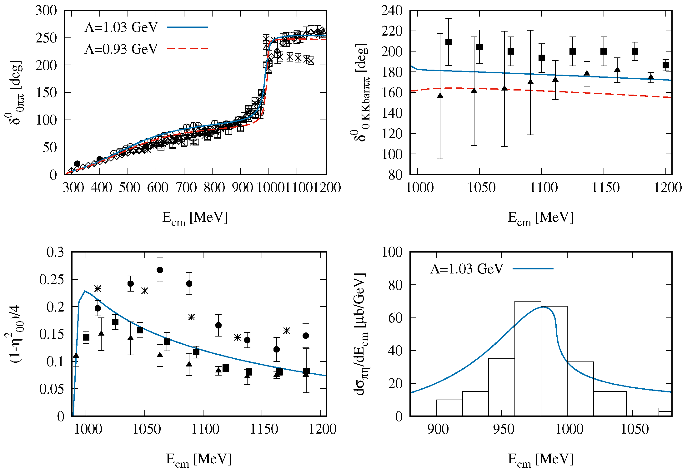
where u and d are the up and down quarks, is their masses, and . Because of the quantum numbers of the non-strange scalar source, the FSI occur in the isoscalar scalar meson-meson scattering, introduced in Section 3. There, we discuss the Adler zero required by chiral symmetry and the pole of the or resonance, being both of them related by unitarity, analyticity and chiral symmetry. At around the two-kaon threshold, MeV, the channel makes a big impact. This energy almost coincides with the sharp emergence of the resonance, which gives rise to a rapid increase of the isoscalar scalar phase shifts , since it is a relatively narrow resonance [25], cf. Figure 2. The elasticity parameter also experiences a sharp reduction as soon as the channel open, since the couples much more to than to [86]. This phenomenon causes an active conversion of the pionic flux into the kaonic one.
The rapid rise of the isoscalar scalar phase shifts, also implies the corresponding rise of the phase of the isoscalar scalar PWA , , because they coincide below the threshold, that is, for . However, above this energy the rise of is interrupted abruptly if , with , while in the opposite case keeps increasing. Quite interestingly, the two situations can be connected by tiny variations in the values of the parameters in the hadronic model, while keeping compatibility with the experimental phase shifts at around the mass.
As a result, there is a jump in the limiting value of because changes by . Thus, in order to keep constant Equation (68) under an increase by in for , it is necessary to increase p by one unit, so that a zero is necessary in that is not present when . For completeness, we also mention that had we required the continuity from to then an extra pole (in the first RS) should be added. This latter scenario can be disregarded in scattering because of the absence of bound states. With respect to the difference between and , as indicated above, the dominates the behavior of the isoscalar scalar meson-meson scattering around 1 GeV, and couples much more strongly to kaons than to pions. For instance, Reference [86] calculates that its coupling to kaons is a factor 3 larger than that to pions. This makes that the mixing between the pion and kaon scalar form factors is suppressed, following each of them its own eigenchannel of the PWAs.
Let be the value of s at which the pion scalar form factor has a zero for . Then, we can write an Omnès representation of the pion scalar form factor in terms of a modified Omnès function
such that . From here it is clear that can be fixed by the requirement that . Because of the Watson final-state theorem in the elastic region we can write that and it vanishes when , which allows to determine from the knowledge of . The context clarifies whether the same symbol actually refers to Equation (57) or Equation (70).
A clear lesson from the discussion here is that possible troubles could occur when using an Omnès function in fitting the free parameters because an unstable behavior could arise due to a jump in . These regions of dramatic differences in are separated by a discontinuity of in the parametric space. As a consequence, it is important in the fitting process to satisfy the condition Equation (68). In particular, for the PWA the more elaborated function in Equation (70) should be used, instead of just the standard Omnès given in Equation (61). This fact also affects studies of two-photon fusion into two pions, like Reference [87], as discussed in Reference [88].
4.2. The IAM for FSI
The first step of Reference [19] is to write down twice subtracted DR expressions for the scalar and vector pion form factors, and , respectively, as
Here, and are the and 1 isoscalar and isovector phase shifts, in this order. These DRs can be interpreted as singular integral equations (IEs) for the form factors and [89].
Let us remark, as in Reference [19], that the solutions of the IEs of Equations (71) and (72) for and , respectively, can be expressed in terms of the associated Omnès functions [90]. In the approximation of identifying the phases of the form factors with the phase shifts, strictly valid only for the elastic region, one has the approximate expressions
where and are polynomials that take into account the zeros (if any) of the form factors in the first or physical RS.
At the one-loop order in ChPT or, equivalently, at next-to-leading order NLO or , we can replace inside the dispersive integrals of Equation (71) the scattering PWAs at leading order,
The phase space function is defined in Equation (2). Evaluating the dispersive integral in Equation (71) with the approximation for of Equation (75), Reference [19] of course ends with the same expression for as the NLO ChPT [7] result,
The function is defined in Equation (28). By proceeding in an analogous way, a similar expression holds for the vector form factor at this level of accuracy, ,
There is an important difference between the scalar and vector form factors. The unitarity corrections are enhanced by around a factor 6 for the former compared to the latter, because the leading order ChPT amplitude is around a factor 6 larger, compared Equations (75) and (76), as first noticed in Reference [26] and already discussed above in detail.
By invoking the Watson final-state theorem, one can calculate from the perturbative expressions of and in Equations (77) and (78) the phase shifts for and 1, respectively. Nonetheless, since the form factors are calculated perturbatively one should proceed consistently in order to extract from this perturbative information the corresponding phase shifts. In this way, denoting by the LO form factors and by their NLO contributions, with the superscripts indicating the real (r) and imaginary (i) parts, we then have for the Watson final-state theorem:
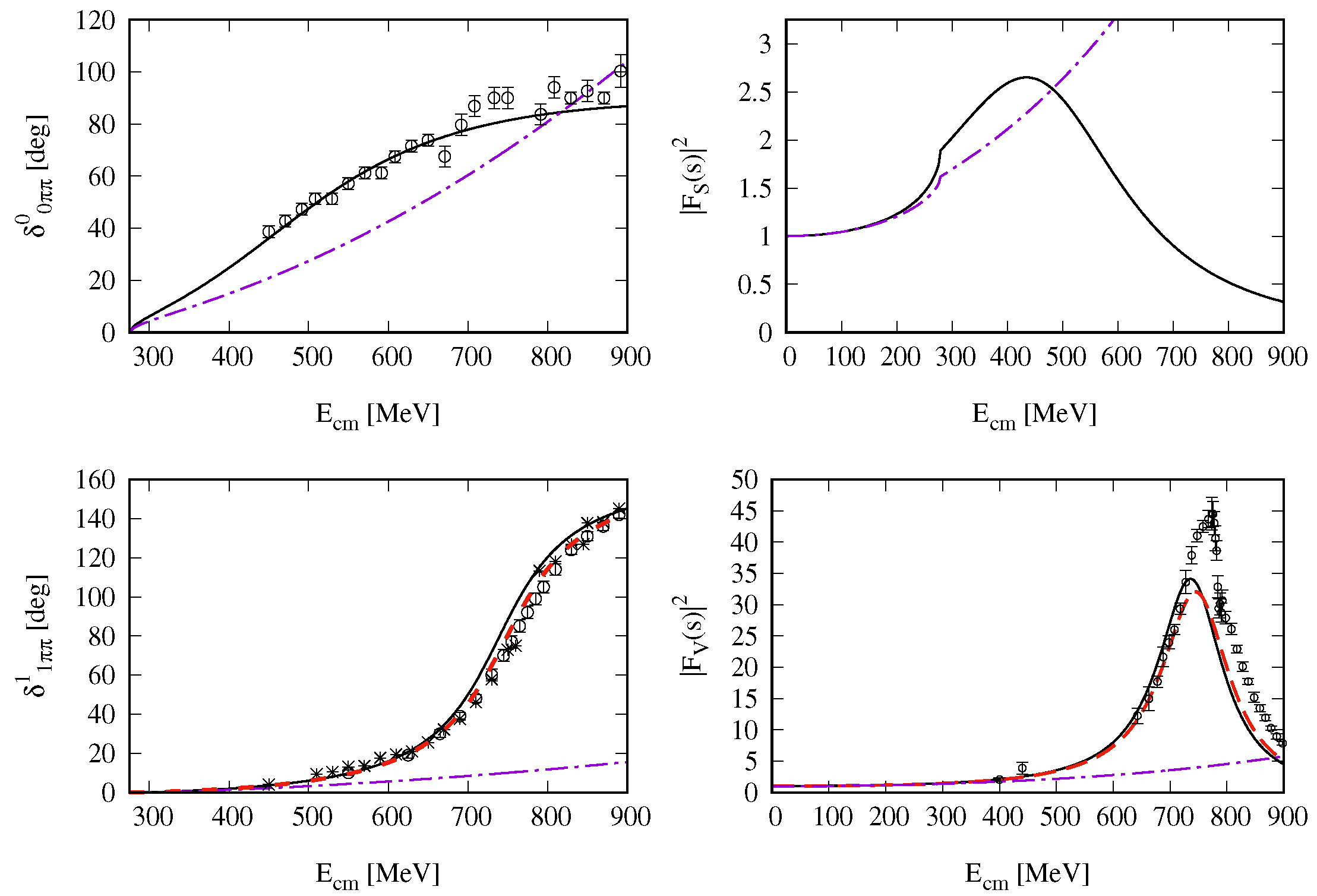
from where the phase can be extracted. Let us notice that Reference [19] compared directly the phase of the perturbative form factors in Equations (77) and (78) with the phase shifts of the PWAs in its Figure 1 and Figure 2. In this respect, it did no take account that this is not meaningful because the Watson final-state theorem only holds perturbatively in ChPT, as explained. We show in Figure 1 the resulting form factors, so that the top line is dedicated to and the bottom one to . The panels on the left correspond to the phases of these form factors and the panels on the right to their module squared. It is clear that there is a strong departure between the calculated phase shifts from the NLO ChPT form factors (magenta dashed lines) and the experimental values even at low values of s. This is also clearly true for the modulus squared of , for which the perturbative calculation again departures strongly from the experimental points. It is particularly visible there the emergence of the resonance , which dominates the phase shifts and , with tails extending up to threshold and affecting the low-energy results. This phenomenon can only be captured approximately in ChPT by the large size of the counterterm ,
as estimated in Reference [7].
For the vector case, the cause of the large higher-order contributions is clearly associated with the prominent role played by the resonance. In turn, for the scalar sector the enhanced RHC is the one blamed for such effects. Indeed, these strong contributions from unitarity and analyticity even drive to the emergence of a pole in the complex s plane, the or resonance, as already discussed, cf. Equation (3).
Reference [19] discusses that the application of the chiral series expansion should be performed on the inverse of the form factor rather than on the form factor itself. The main reason lies on sound and general grounds, as provided by unitarity and analyticity. Let us consider a DR representation of , analogous to Equation (71). The point to be stressed is that the imaginary part of is expected to be much smoother than the imaginary part of itself in the elastic region. The reason is that the imaginary part of the inverse of the form factor satisfies, because of unitarity in PWAs, that
As and share the same resonances, their propagators cancel in the ratio that gives . Then, this ratio is expected to be smoother than , where this cancellation does not occur but rather the resonance effects in and mutually enhance each other because of the product involved.
Then, let us write down a twice-subtracted DR for the inverses of the form factors and . First, we neglect by now the possible presence of zeroes in the form factors in the 1st Riemann sheet (RS), which give rise to poles in the inverse of the form factors. The issue of a zero in for certain types of T matrices was already discussed in Section 4.1, as first shown to happen in Reference [85]. This is not an issue here because we are considering the one-channel elastic scattering in the isoscalar scalar PWAs. As a result we write,
Then, up to , in the integrand of these integrals one takes the leading order expressions in the chiral expansion of , cf. Equations (75) and (76), and . In this way, except for a global sign the same result as above is obtained for the dispersive integral as in the DR for . Namely, the only difference is a flip of sign in the NLO contributions in Equations (77) and (78). Then, the results for the form factors can be written as
with representing either or and is the ChPT result. Similarly is the LO ChPT calculation. Being more specific, Equation (84) results after performing the DR integrals, compare with Equations (71) and (72),
The resulting phase and modulus squared of from Equation (85) is shown by the (black) solid lines in the top panels of Figure 1. The resummed expression of in Equation (86) gives rise to the results shown by the (black) solid and the (red) dashed lines in the bottom panels of Figure 1. They differ in the value of employed, so that the former uses 0.42 fm (as in Reference [19]), and the latter takes the slightly lower value 0.41 fm, so as to agree better with the data on the isovector vector phase shifts. We also use the updated value MeV, instead of 94 MeV used in Ref. [19] (this reference indeed employs the normalization MeV = ). It is clear that now, the resulting phase shifts calculated from the phases of the form factors in Equations (85) and (86) are much closer to the experimental points than the perturbative ones form Equations (77) and (78). The same dramatic improvement also happens for the modulus squared of calculated from Equation (86), as compared with the data points given by the empty circles. In the peak of it is clear the effect due to the mixing, which is not treated here, see for example, Reference [94] for its implementation. Notice that this improvement is achieved by employing the same perturbative input, namely the NLO ChPT results. It is a matter of properly reshuffling the chiral expansion in a way clearly motivated by unitarity and analyticity. We also show in the right top panel of Figure 1, in which the resonance shape due to the is clearly visible. These resonance effects are not so evident in the case of the isoscalar scalar phase shifts because of the Adler zero in this PWA, which interferes strongly with the pole contribution from the resonance itself.
4.3. KT Formalism
The KT formalism was originally developed by Reference [21] to study the decays and, up to including two-body intermediate states, it allows to implement unitarity and crossing symmetry. Later on, this approach has been applied to study extensively the decays, among others. These decays violate isospin because the G parity of the is and that of the pion in , so that it is proportional to in pure QCD.
The application of ChPT to the decays has been controversial, until accepting that FSI are so strong that a non-perturbative unitarization method is needed to be implemented in order to be able to confront well with experimental data [18]. The earliest calculations using current-algebra techniques obtained a value for the of around 65 eV [95], too small compared with the experimental result eV [25]. Roiesnel and Truong [18] stressed that a non-perturbative calculation taking care of the isoscalar-scalar FSI, by employing an Omnès function on top of the current-algebra result, increases the decay width up to 200 eV. A few years later, the NLO ChPT calculation [96] gives eV, which implies a large correction by a factor 2.4 over the LO calculation in the right direction, but still too small by around a factor of 2. In addition, the parameter , typically employed in the parameterization of the Dalitz plot for the decay , is positive at NLO ChPT [96] while experimentally it is negative, [25]. The calculation at NNLO in ChPT of the decays was performed in Reference [97] but the proliferation of new counterterms prevented a sharp result. If resonance saturation is assumed to estimate the NNLO ChPT counterterms then the Dalitz plot parameters are not well reproduced. One then concludes that the decays are sensitive to the detailed values of the counterterms, so that an accurate calculation requires a precise knowledge of their values. This controversial situation stimulated the interest in developing sophisticated calculations combining ChPT and non-perturbative methods, within unitarized ChPT [18,98,99] and the KT formalism [100,101,102,103,104].
We now describe the basic points of the one-channel KT formalism for decays and refer the reader to References [104,105] and the recent review in Reference [67] for further details. In particular, the generalization to coupled channels was worked out in Reference [104], given in a more compact matrix notation in Reference [67].
Let us consider the decay , which is related by crossing symmetry to the scattering reactions in the s-channel, in the t-channel, and in the u-channel. The Mandelstam variables s, t and u are given by
The crossing-symmetry relations are
These amplitudes in turn can be decomposed in scattering amplitudes with well defined isospin, , as
The inversion of these relations gives us the ,
The PWA amplitudes are denoted by , and one has the standard relations
In the KT formalism the S and P waves are the ones that are subject to a non-perturbative treatment.
The PWAs have a RHC above the two-pion threshold . Instead of writing the unitarity constraint as in Equation (18), one should consider it as giving the discontinuity along the RHC because of the two on-shell intermediate pions. Due to the fact that in the decay channel all the three pions are on-shell in the region this is another source of imaginary part from the crossed-channel cuts that are also on-shell. For the branch point singularity at happens for . These crossed-channel cuts can be separated from the RHC one by giving a vanishing positive imaginary part to and then proceed by analytical continuation in [106]. We then write
From the last line in Equation (92) we can write more conveniently the discontinuity of along the RHC, , as
which is the relation finally used.
A crucial feature of the KT formalism is to write down as the sum of three functions of only one Mandelstam variable, , and [103,104]
which is invariant under the exchange , a feature that can be seen as a consequence of charge-conjugate invariance. This representation is valid up to in ChPT [97,103] because then the D waves also contribute and higher polynomials in and would be required. The derivation of Equation (94) can be understood by considering only PWAs in the s-channel and taking into account the isospin decomposition for the process and the crossed-channel ones, cf. Equation (89). In this way, for the s-channel process there is no contribution, which only happens in the crossed ones, cf. Equation (89). As this is a P-wave we then write it as , that also keeps explicitly the symmetry under the exchange . The contribution can only happen in the s-channel, because for the other channels the third component of isospin is not zero. This is the contribution in Equation (94). Finally, regarding the it is clear from Equation (89) that it appears in the combination .
Taking the expression for in the ones of , as given in Equation (90), it follows that
Writing down the PWAs for and 11 we have
where
with
We have also introduced in Equation (96) the angular averages
and
The function has no discontinuity across the RHC so that the discontinuities of the PWAs can be expressed as,
Following the same steps as above in Equation (93) we can then also write that
with except for for which (as it should be clear from the context in this section). Dividing this expression by the corresponding Omnès function , which fulfills that along the RHC , , we then obtain from Equation (102) the discontinuity of as
The final step is to obtain IEs for by writing down DRs for as
where is a subtractive polynomial with . Requiring that diverges linearly at most at infinity in the Mandelstam variables [101], then should be bounded by a constant and , would diverge linearly at most in the limit . Furthermore, we also know the asymptotic behavior in the same limit for the Omnès functions, cf. Equation (65), with . Depending on the value of m should be adjusted to the required asymptotic behavior of . For instance, Reference [104] assumes that , and , so that for and for and 2.
The DRs in Equation (104) constitute a set of coupled linear IEs because the angular averages are also expressed in terms of the functions. A standard way for solving these equations is by iteration. The subtraction constants can be determined by matching with the NLO ChPT calculation of and/or fitted to data, as done in References [101,104]. A clear improvement is obtained in the calculated decay width for the in Reference [101], where the value eV was obtained. Other improvements concern the parameter for characterizing the amplitude for in its Dalitz plot. NLO ChPT gives a value while the KT treatment of Reference [104] gives , to be compared with the PDG average value of .
5. The Method
In this section we elaborate on different aspects of the method, first introduced in Reference [16] to study uncoupled PWAs. We first review on this method, discuss in more detail the limit in which the crossed-channel dynamics is neglected [26], and afterwards elaborate on how the latter can be treated perturbatively within the method [39,107]. These results can also be used to take into account FSI in production processes [94,108]. For the case of NR scattering, thanks to recent developments [35], it is possible to know the exact discontinuity of a PWA along the LHC for a given potential. In this way, one can generate the same solutions as in the Lippmann-Schwinger (LS) equation, together with other ones that cannot be obtained in a LS equation when mimicking the short-distance interactions by contact terms in the potential [36].
5.1. Scattering
For the scattering of particles with equal masses there is only a LHC for because of crossing. However, when the particles involved have different masses there are also other types of cuts in the complex s plane due to crossing. For instance, for the scattering of particles , in addition to a LHC there is also a circular cut for [65] where, for definiteness, we have considered that . Nonetheless, when we refer in the following to the LHC we actually mean all the crossed-channel cuts. Indeed, had we taken instead the complex plane all the cuts would be linear and only a LHC would be present [65].
We introduce the method following Reference [26]. The uncoupled case is discussed first and afterwards we move to coupled-channel scattering. The discussion is restricted to two-body intermediate states. The discontinuity of the inverse of a PWA along the RHC is times its imaginary part, being the latter fixed by phase space because of unitarity, cf. Equation (17).
In the method is expressed as the quotient of two functions,
where stands for the numerator function and for the denominator one. The former has only LHC and the later RHC.
To enforce the right kinematical threshold behavior of a PWA, vanishing as , Reference [26] divides by ,
The method is then applied to this function,
It follows then that the discontinuities of and along the LHC and RHC, respectively, are
with along the LHC. Let us discuss the DRs for and that result by taking into account these discontinuities. For one has,
Here n is, at least, the minimum number of subtractions required to guarantee the convergence of the integral in the DR,
Consistently with Equation (111), the DR for can be written as
The Equations (110) and (112) are a system of coupled linear IEs whose input is . It is customary to substitute the expression for in and end with a linear IE for along the LHC. Namely,
and the last integral can indeed be performed algebraically. This is a linear IE for with s along the LHC. Once this solved one can calculate for and, in particular, along the physical region, . Other types of IEs could be deduced by taking more subtractions independently in and . Fore more details on this respect the reader can consult [109].
The expression in Equation (113) can be shortened and simplified for equal mass scattering with mass m by taking , because then . It follows that,
The last integral in the previous expression can be written in terms of , Equation (2).
One of the subtraction constants can be fixed because we can freely choose the normalization of , since their ratio and analytical properties are invariant under a change in normalization. The standard choice is to take . However, given along the LHC, the solution is not unique because of the addition of extra subtraction constants in and .
Historically, the possible addition of Castillejo-Dalitz-Dyson (CDD) poles [110] was the clear indication that extra solutions could be obtained even if is assumed to be known along the LHC. They give rise to zeros of along the RHC and each zero comprises two real parameters, its residue and position. Phenomenologically the CDD poles correspond to the short-distance dynamics underneath the scattering process and might also be related to the addition of bare states [111]. Let us notice that does not exist at a zero of and, therefore, Equation (17) is not defined there. As in Reference [110] let us introduce the auxiliary function such that
and rewrite Equation (108) as,
Denoting by the zeros of along the real axis above threshold, we can write from Equation (116) as
where the are a priori unknown. Thus, Equations (115) and (117) allow us to write
The last term in the previous equation can be rewritten as
The contribution can be reabsorbed in and Equation (118) can be rewritten as
where , and are constants not fixed by the knowledge of , and the CDD poles give rise to the last term.
Interesting results can be deduced under the approximation of neglecting the LHC, . Equation (112) then becomes
and is just a polynomial, which can be reabsorbed in by dividing simultaneously both functions by itself. The expression for then becomes
The number of real free parameters in the previous equation is , with the number of CDD poles. A priori there is nothing to prevent the generalization of Equation (122) such that some could also lie below threshold. We could adjust the position and residue of a CDD pole such that the real part of vanishes at the desired position. This would give rise to typical resonance behavior above threshold, or to a bound-state pole if this happens below threshold. This is why the parameters of the CDD poles are typically associated with the coupling constants and masses of the poles in the S matrix. In other instances, the CDD poles are needed because the presence of a zero cannot be related to , but they respond to fundamental constraints in the theory. This is the case of the Adler zeroes in QCD [69], which already occur at LO in the chiral expansion, while only at NLO and higher orders. It is therefore necessary to account for them by including CDD poles, such that the derivative of the PWA at the zero corresponds to the inverse of the residue of the CDD pole, . For the Adler zeroes the latter could be fixed in good approximation by the LO ChPT result. The other parameters emerge by having enforced the correct behavior of a PWA near threshold, which should vanish as .
Let us stress that Equation (122) gives the general form of an elastic PWA when the LHC contributions are neglected. Phenomenologically this assumption could be suited if the LHC is far away and/or if it is suppressed for some reason [112,113]. The free parameters in Equation (122) can be fixed by fitting experimental data and/or by reproducing the Lattice QCD (LQCD) results at finite volume or when varying some of the QCD parameters, like or the quark masses [114,115,116,117].
Reference [26] focuses on meson-meson scattering, whose basic theory is QCD. It studied the S- and P-wave two-body scattering between the lightest pseudoscalars (, K and ), as well as the related spectroscopy. It was found that the full nonet of scalar resonances [118] , , and arose from the self-interactions among the lightest pseudoscalars, while the more massive resonances , , and stem from a nonet of bare resonances with a mass around 1.4 GeV. In addition, Reference [26] included a bare scalar singlet with a mass around 1 GeV which gives also a contribution to the [119]. Later on, Reference [120] extended this model by including more channels and could determine a glueball state affecting mainly the with a reflection (because of the threshold) on the as well. Of course, the same Equation (122) can be applied to other interactions, for example, Reference [107] studied scattering in the electroweak symmetry breaking sector.
The generalization of Equation (122) to coupled channels is rather straightforward by employing a matrix notation, where the T matrix in coupled channels is a matrix denoted by . As in Equation (122) we take from the onset that crossed-channel dynamics can be neglected in a first approximation. Thus, the matrix element is proportional to , which gives rise for odd orbital angular momentum (unless ) to another cut between and due to the square roots in the expressions of and as a function of s. To avoid this cut we define the matrix , analogously to Equation (106), as
In this equation, the symbol corresponds to a diagonal matrix with matrix elements
and and are the masses of the two particles in the same channel i. The matrix unitarity relation along the RHC then reads
where is another diagonal matrix whose elements are . The next step proceeds with the generalization to coupled channel of Equation (105) by writing as
with and two matrices, the former only involves LHC and the later RHC, respectively. In our present case without LHC, the matrix elements of are polynomials functions. Multiplying and in Equation (126) to the left by we can always make that and write,
with a matrix of rational functions which poles produce the CDD poles in . Let us notice that all the zeros in correspond to CDD poles in the . This is the generalization of the CDD poles for the coupled-channel case.
The resulting expression for in Equation (127) can be also recast as
with the diagonal matrix with matrix elements defined as
where is a subtraction constant and the subtraction point. The result of this integration can also be written as
The parameter is a renormalization scale, such that a change in the value of can always be reabsorbed in a corresponding variation of , while the combination is independent of . The unitarity loop function corresponds to the one-loop two-point function
where and the total four-momentum is indicated by P. The integral in Equation (131) diverges logarithmically, which is the reason why a subtraction has been taken in Equation (129). The Equation (130) also results by employing dimensional regularization and reabsorbing the diverging term in .
Let us elaborate on the so-called natural value for the subtraction constants. The function given by Equation (130) has the value at threshold,
This expression is compared with the one that results by evaluating in terms of a three-momentum cutoff . The resulting expression for the function , and denoted by , can be found in Reference [79]. The natural size of a three-momentum cutoff in hadron physics is the inverse of the typical size of a compact hadron, which is generated by the strong dynamics binding quarks and gluons. Thus, according to this estimate we take GeV. For NR scattering and () are given by the value at threshold of every function plus [109]. The value at threshold of can be worked out explicitly with the result [114]
By equating Equations (132) and (133) the following matching value for results,
One should employ GeV in Equation (134) to estimate the natural value for the subtraction constants, a procedure originally established in Reference [39]. In this way, both the renormalization scale and the cut off are used with values suitable to the transition from the low-energy EFT to the shorter-range QCD degrees of freedom. As an example, let us take scattering and GeV. Then, from Equation (134)
The Equation (128) is adequate for including perturbatively the LHC contributions in the T-matrix . This can be achieved by matching order by order with a calculation within an EFT. For instance, this has been used many times taking as input one-loop calculations in ChPT [39,86,107,114,115,121,122,123,124,125,126]. The procedure is as follows. Let us take a meson-meson scattering amplitude calculated in ChPT up to one-loop or , . Then the chiral expansion of Equation (128), with , [107], reads at LO,
and at NLO,
and similarly for higher orders. Thus, up to NLO the matching equations fix and to
The LHC contributions arise because crossed-channel loops are calculated order by order in the ChPT results for . At NLO in the calculation of we then have the expression
If is further expanded we then recover the IAM result of Equation (39) because
so that
This is the formula for the IAM in coupled channels at NLO [79,127].
In order to appreciate the power of the method for some reactions we consider the LO matching, that is, with , applied in Reference [27] to study the meson-meson S-waves with and 1. This is a coupled-channel study with and for and and for . It is certainly remarkable that only one free parameter entered in the successful calculation of the PWAs from the threshold up to around 1.2 GeV. This is shown in Figure 2 by the , phase shifts, the inelastic reaction and a event distribution around the , from top to bottom and left to right, respectively. The resonances , and , clearly visible in Figure 2, are generated dynamically from the interactions between the pseudoscalars. The free parameter is the three-momentum cut-off with natural size GeV used in the evaluation of the unitarity-loop functions employed in this study.
It is also the case in some instances [26,86,114,115,120,121] that the ChPT expansion is complemented with the exchange of bare resonance fields, so that the tree-level amplitude is crossing symmetric. One typically improves the convergence properties of the chiral expansion by including bare resonance fields because of the (partial) saturation of the chiral counterterms by the resonance exchanges [128]. Then, the matching process is undertaken up to , which means to neglect any two-loop contribution and any one-loop contribution beyond . In this way, one could consider one-loop contributions involving higher orders because of the explicit inclusion of the resonance fields. The matching proceeds as in Equations (136) and (137), with the difference that now the LO amplitudes include also the tree-level exchange of resonances and involves the one-loop contributions up to . Then, the Equation (138) still holds and one has again Equation (128) for . This equation is in appearance analogous to the -method form of Equation (126). Indeed, if we identify with and with , it can be shown [129] that up to the resulting functions satisfy the -method equations, cf. Equation (108).
The perturbative solution of the equations with respect to the LHC contributions can also be organized as an iterative solution in increasing number of insertions of . The first-iterated method consists on taking only one power of in the integrand of the DRs for and . The approximation is obtained by settling into the integrand for the DR of , Equation (112), which is then denoted as . Then,
Since is known the DR integral could in principle be calculated. This is usually a tree-level amplitude that can also be calculated in QFT, from which indeed is actually derived. Therefore, we assume that in the first iterated method is also given. As a result, the calculation of in this approximation, denoted by , just reduces to perform the integration
The first-iterated method was used in Reference [130] to discuss scattering within linear realizations of chiral symmetry, taking into account the exchanges of a and resonances. More recently, it has been employed to study scattering in Reference [131] by taking the pure gauge-boson part of the non-linear chiral Lagrangian with hidden-local symmetry [132,133]. Its generalization to the -related vector-vector scattering was undertaken in Reference [134]. These studies were motivated by the earlier ones in References [135,136,137,138], with still an on-going productive discussion in interpreting the results.
5.2. FSI
Let us consider the unitarity relation for a form factor, Equation (23), with the expression of the T matrix in PWAs as given in Equation (128). It then results that
Since it is clear that , so that from Equation (144) we have that along the RHC it is fulfilled that
The cancellation of from both sides leads to
From this equation it is clear that the combination
has no RHC [139]. Then can be expressed as
with a column vector of n functions without RHC, being n the number of PWAs.
An analogous relation can be obtained if we write as in the method in coupled channels, . Following the same steps as in Equations (144)–(148), taking into account that , one ends with the relations
and is free of RHC. We can then write as the product of two matrices, the inverse of , which only has RHC, and , which could have LHC. As a result, Equation (149) is the generalization of the method to production processes.
Coming back to Equation (148), let us remark that could have the two types of cuts (since in general has LHC). For instance, for the case of the pion form factor if this is expressed as in Equation (149) then has no LHC, while if expressed as in Equation (148) it would typically have one, if has it. However, for the relevant case for phenomenological applications in which is driven by the s-channel dynamics and it does not comprise explicit LHC, then has no either LHC. In this case, the matrix and can be identified.
This formalism has been employed by Reference [140] to study the meson-meson fusion reactions. References [108,141] used it to study the scalar form factor of the pion (and of other pseudoscalar mesons) in connection with and D decays, and Reference [94] analyzed the vector form factor of the pion. This formalism was also very important to unveil the two-pole structure of the in Reference [39], because in previous studies the event distribution for this resonance was always taken to be proportional to the modulus squared of the S-wave.
5.3. The Exact Method in NR Scattering
For non-relativistic scattering one can calculate for a given potential the exact discontinuity of a PWA along the LHC. This has been a recent advance in S-matrix theory achieved by Reference [35], to which we refer the reader for further details. The key point was to extrapolate analytically the LS equation to complex three-momenta for off-shell scattering. The solution of the LS equation for half-off-shell scattering is an analytical function in the off-shell three-momentum complex q plane with vertical cuts which extend along the lines , with . Here the ± symbols are unrelated, is the lightest particle exchanged, and p is the on-shell three-momentum (fixed by the energy E of the process, , with the reduced mass). for example, for scattering the lightest particle exchange is the pion and . We denote in the following a PWA for half-off-shell scattering as , where q is the off-shell three-momentum and p the on-shell one.
The discontinuity we are interested in, for example, for its later application to the method, is
After some mathematical derivations that can be consulted in Reference [35], this discontinuity can be obtained by solving an ordinary linear IE. This IE is written in terms of the discontinuity of the potential in momentum space . Its writing gets simplified by using defined by
The discontinuity of the potential entering into the IE is
with and at the end of the calculation. After this preamble, the sought IE is (, and )
In terms of the discontinuity is given by
Thus, we need to solve the IE for , and the range of the integration in the IE for is finite for a given p, contrary to the LS equation. This IE can be solved without ambiguity because can be determined for a given potential and with it by solving Equation (153).
For a general potential it is convenient to employ its spectral decomposition,
where is the spectral function, and the ellipsis indicates possible subtractions that due to its polynomial nature do not give contribution to the discontinuity of the potential. In terms of the spectral decomposition we can write that
The function is a polynomial in its argument and its fixed by the partial-wave projection involved in the case of interest. For brevity in the presentation offered here we have just referred to the uncoupled case, but the formalism can also be generalized easily to evaluate the LHC discontinuity for coupled PWAs [35].
A potential is said to be singular if for it diverges stronger than or as for . In the opposite case the potential is said to be regular [35]. In the ChPT calculation of nuclear potentials the increase in the order of the calculation implies typically an increase in the degree of divergence of the potential for , because off-shell momentum factors give rise to spatial derivatives. This fact is the main reason why the original Weinberg’s program for solving nuclear properties once the chiral potentials are calculated order by order has not been taken to full completion.
The resulting obtained by solving the master Equation (153) has a different qualitative behavior depending on whether the potential is regular, attractive singular or repulsive singular. General arguments, based on the scaling properties of the function , were given in Reference [35] to explain such differences in the behavior of . Explicit examples were also worked out in Reference [35] corresponding to actual PWAs in scattering, with the chiral potential calculated at different chiral orders, from LO up to NNLO. The function is a polynomial in and of degree m. Then, the argument of Reference [35] follows by considering a re-scaling by a parameter of the variables k, and in the limit . It follows from Equation (153) that the iterated solution for is subject to a re-scaling by
The point is whether is smaller or larger than zero. In the former case we have the behavior corresponding to a regular potential, so that each extra iteration implies at least an extra factor of and for the discontinuity tends to its Born approximation. However, when each iteration increases the power of k in the asymptotic behavior of , becoming more and more divergent as n increases. This is the situation for a singular potential.
For the regular potentials tends to its Born term contribution which vanishes at least as for and . For such type of it was shown in Reference [109] that any IE, irrespectively of the number of subtractions taken, has solution. However, for singular potentials the resulting grows faster than any polynomial in the same limit. This is clearly shown in Reference [35] by log-log plots in which the slop of continuously grows with increasing . As a dramatic consequence of this result is that it is not possible to write down a DR representation for a NR PWA if the potential is singular. However, it is still possible to use the method because what matters for the IEs is the product . The denominator function is known to behave asymptotically as , cf. Equation (65), and , with N the number of bound states, because of the Levinson theorem. It turns out that the number of such stats is infinite for attractive singular potentials [142] and, in this case, vanishes also faster than any power law.
The exact method is defined in Reference [35] as the method but using stemming from Equations (153) and (154), which is the exact LHC discontinuity of the full PWA for a given potential. In this way, we showed in Reference [35] that one reproduces exactly the LS-equation solutions for regular potentials. This is also true for the singular potentials when the potential is used in the whole range of integration in the LS equation, that is, for (the cut-off is sent to infinity). For the singular-potential case we refer to the standard kind of solutions, so that for a repulsive singular potential the solution has no free parameters and is determined, while for the attractive singular case the solution involves one free parameter that could be fixed for example, by imposing a given value for the scattering length [142,143,144,145,146]. Several potentials were studied in Reference [35], both for uncoupled and coupled PWAs. Within the latter group the – coupled PWAs were studied and the scattering length was taken as input. Needless to say, in all cases the LS equation with infinite cutoff and the method agree perfectly in our numerical study.
The fact of having none or only one free parameter is a very constrained situation in practical applications, and it is the reason why it has not been possible to achieve yet a good agreement with data in scattering in terms of regulator-independent solutions (i.e., in which the three-momentum cut-off is taken to infinity). Notice that the number of free parameters in the solution of the LS equation for singular potentials is then not linked with the chiral order in the calculation of the chiral potential. However, in terms of the method one can in principle add an arbitrary number of subtractions, which allows one to look for extra solutions. We have already discussed this point in connection with the ambiguity associated with the CDD poles in Section 5.1. This possibility was explored in detail in Reference [36] for the PWA. The NLO and NNLO ChPT potentials for this PWA are actually attractive and singular. The standard solutions of the LS equation were reproduced, and a detailed numerical analysis was performed in order to show the agreement between the LS equation and the exact method. But we also showed in this reference that one can generate new solutions that cannot be achieved by the LS equation when the three-momentum cut-off is taken to infinity with contact interactions included in the potential to aim renormalization (in the form of polynomial counterterms in its momentum expression). In this way, a new solution was discussed that can reproduce the scattering length, effective range and shape parameter . For this solution the DRs for and converge separately. It is also interesting to indicate that a solution within the exact method for this PWA fixing only two parameters, the scattering length and the effective range were taken, could not be found. Last but not least, a very attractive feature of the exact method is that it allows to evaluate the PWAs in the whole complex plane. Then, it is very convenient to look for resonance and (anti)bound states. In the case of the PWA there is an antibound state which is found at MeV both at NLO and NNLO when all the first three ERE parameters are reproduced.
6. Conclusions
We have elaborated on several unitarization methods of perturbative calculations in Chiral Perturbation Theory (ChPT) that can be employed to study scattering and the re-scattering corrections to an external probe. Special attention has been given to the method both for scattering and for implementing the final-state interactions (FSI). The unitarization methods, since the earlier papers on current algebra techniques, have been able to extend to much larger energies the expected region of utility of ChPT calculations. This has been accomplished thanks to the extra energy and momentum dependence generated by using a non-perturbative theoretical framework which satisfies key properties of S-matrix theory, which stem from two-body unitarity and analyticity. Some of the most striking and important applications of the unitarization methods of input perturbative calculations have occurred in the field of spectroscopy. In this way, it has been possible to study resonances and bound states, and even predict some of them, while unexpected properties have been unveiled too, as for example, the two-pole nature of some resonances [147], as first shown for the in Reference [39].
Along this review we have paid attention to establish links between different unitarization methods. Thereby, by starting with the (generalized) relativistic effective-range expansion (ERE) we have connected it with the K-matrix approach and then obtained from the former the Inverse Amplitude Method (IAM) unitarization formula. The IAM has been also connected with the Paddé approximation. In the last part of the manuscript we have introduced and discussed the method. A link between the and the IAM can also be established by employing the solution to the method based on treating perturbatively the left-hand cut discontinuity. This allows one to derive the IAM as a particular case of this method too. The associated methods to take care of the FSI corresponding to the unitarization techniques of scattering have been introduced as well. In addition, we have discussed the (Muskhelishvili-)Omnés solution and the Khuri-Treiman approach.
An advantage of the unitarization technique based on the method is that it can be applied to deliver the unitarized partial-wave amplitudes (PWAs) even if only the leading-order scattering amplitudes are employed. A subtraction constant is then required, but it could be estimated making use of naturalness arguments. In this way, one can study important resonances in hadron physics in a very constrained manner, essentially without any free parameter. Good examples are the , , , and in the scalar light mesonic sector, the in the strangeness S-wave meson-baryon scattering, and so forth. Of course, one could also use as input higher-order scattering amplitudes provided by the effective field theory of interest and perform a higher-order analysis in the input taken.
Regarding the method, we would like to stress that thanks to recent advances (in which the author has been involved), it can be considered for non-relativistic scattering as an alternative formulation of scattering theory. The qualitative leap forward has been the derivation of the exact discontinuity of a PWA along the left-hand cut, which can then be employed to solve the integral equations. In this way, one can solve standard regular potentials and reproduce the solutions obtained with the Lippmann-Schwinger equation for PWAs. But it also allows to obtain extra solutions for singular potentials without dependence on cutoff, which can be sent to infinity. This method has the advantage that, in terms of the solution found, it is straightforward to evaluate the on-shell scattering amplitudes in the complex energy plane too. In this way, for example, one could look for poles and their residues (which give the resonance or bound-state couplings). This is a very promising and exciting field of current research, and first applications are being explored for scattering.
Funding
This research received no external funding.
Acknowledgments
This work has been supported in part by the MEC (Spain) and FEDER (EU) Grants FPA2016-77313-P and PID2019-106080GB-C22.
Conflicts of Interest
The author declares no conflict of interest.
References
- Coleman, S.; Wess, J.; Zumino, B. Structure of Phenomenological Lagrangians. I. Phys. Rev. 1969, 177, 2239. [Google Scholar] [CrossRef]
- Callan, C.G.; Coleman, S.; Wess, J.; Zumino, B. Structure of Phenomenological Lagrangians. II. Phys. Rev. 1969, 177, 2247. [Google Scholar] [CrossRef]
- Weinberg, S. Dynamical approach to current algebra. Phys. Rev. Lett. 1967, 18, 188. [Google Scholar] [CrossRef]
- Schwinger, J. Chiral dynamics. Phys. Lett. B 1967, 24, 473. [Google Scholar] [CrossRef]
- Wess, J.; Zumino, B. Lagrangian method for chiral symmetries. Phys. Rev. 1967, 163, 1722. [Google Scholar] [CrossRef]
- Gasiorowicz, S.; Geffen, D. Effective Lagrangians and field algebras with chiral symmetry. Rev. Mod. Phys. 1969, 41, 531. [Google Scholar] [CrossRef]
- Gasser, J.; Leutwyler, H. Chiral Perturbation Theory to One Loop. Ann. Phys. 1984, 158, 142. [Google Scholar] [CrossRef] [Green Version]
- Ecker, G. Chiral perturbation theory. Prog. Part. Nucl. Phys. 1995, 35, 1. [Google Scholar] [CrossRef] [Green Version]
- Pich, A. Chiral perturbation theory. Rept. Prog. Phys. 1995, 58, 563. [Google Scholar] [CrossRef] [Green Version]
- Bernard, V.; Meißner, U.-G. Chiral perturbation theory. Ann. Rev. Nucl. Part. Sci. 2007, 57, 33. [Google Scholar] [CrossRef] [Green Version]
- Peskin, M.E.; Schroeder, D.V. An Introduction to Quantum Field Theory; CRC Press: Boca Raton, FL, USA, 1995. [Google Scholar]
- Schnitzer, H.J. Current algebra and unitarity. Phys. Rev. Lett. 1970, 24, 1384. [Google Scholar] [CrossRef]
- Schnitzer, H.J. Current algebra beyond the tree approximation. Phys. Rev. D 1970, 2, 1621. [Google Scholar] [CrossRef]
- Brown, L.S.; Goble, R.L. Pion-Pion Scattering, Current Algebra, Unitarity, and the Width of the Rho Meson. Phys. Rev. Lett. 1968, 20, 346. [Google Scholar] [CrossRef]
- Weinberg, S. Pion scattering lengths. Phys. Rev. Lett. 1966, 17, 616. [Google Scholar] [CrossRef]
- Chew, G.F.; Mandelstam, S. Theory of the low-energy pion-pion interaction. Phys. Rev. 1960, 119, 467. [Google Scholar] [CrossRef]
- Lehmann, H. Chiral invariance and effective range expansion for pion pion scattering. Phys. Lett. 1972, 41, 529. [Google Scholar] [CrossRef]
- Roiesnel, C.; Truong, T.N. Resolution of the η → 3π Problem. Nucl. Phys. B 1981, 187, 293. [Google Scholar] [CrossRef]
- Truong, T.N. Chiral Perturbation Theory and Final State Theorem. Phys. Rev. Lett. 1988, 61, 2526. [Google Scholar] [CrossRef]
- Truong, T.N. Remarks on the unitarization methods. Phys. Rev. Lett. 1991, 67, 2260. [Google Scholar] [CrossRef]
- Khuri, N.N.; Treiman, S.B. Pion-pion scattering and K+/- → 3π decay. Phys. Rev. 1960, 119, 1115. [Google Scholar] [CrossRef]
- Oller, J.A. A Brief Introduction to Dispersion Relations. With Modern Applications; Springer Briefs in Physics; Springer: Heidelberg, Germany, 2019. [Google Scholar]
- Muskhelishvili, W.I. Singular Integral Equations; Springer: Amsterdam, The Netherlands, 1958. [Google Scholar]
- Watson, K.M. Some general relations between the photoproduction and scattering of π mesons. Phys. Rev. 1955, 95, 228. [Google Scholar] [CrossRef]
- Tanabashi, M. Particle Data Group. Phys. Rev. D 2018, 98, 030001. [Google Scholar] [CrossRef] [Green Version]
- Oller, J.A.; Oset, E. N/D description of two meson amplitudes and chiral symmetry. Phys. Rev. D 1999, 60, 074023. [Google Scholar] [CrossRef] [Green Version]
- Oller, J.A.; Oset, E. Chiral symmetry amplitudes in the S wave isoscalar and isovector channels and the σ, f0(980), a0(980) scalar mesons. Nucl. Phys. A 1997, 620, 438. [Google Scholar] [CrossRef] [Green Version]
- Roy, S.M. Exact integral equation for pion-pion scattering involving only physical region partial waves. Phys. Lett. B 1971, 36, 353. [Google Scholar] [CrossRef] [Green Version]
- Ananthanarayan, B.; Colangelo, G.; Gasser, J.; Leutwyler, H. Roy equation analysis of ππ scattering. Phys. Rep. 2001, 353, 207. [Google Scholar] [CrossRef] [Green Version]
- Colangelo, G.; Gasser, J.; Leutwyler, H. ππ scattering. Nucl. Phys. B 2001, 603, 125. [Google Scholar] [CrossRef]
- Kaminski, R.; García-Martín, R.; Grynkiewicz, P.; Peláez, J.R.; Ynduráin, F.J. New dispersion relations in the description of pi pi scattering amplitudes. Int. J. Mod. Phys. A 2009, 24, 402. [Google Scholar] [CrossRef] [Green Version]
- García-Martín, R.; Kaminski, R.; Peláez, J.R.; Ruiz de Elvira, J.; Ynduráin, F.J. The pion-pion scattering amplitude. IV: Improved analysis with once subtracted Roy-like equations up to 1100 MeV. Phys. Rev. D 2011, 83, 074004. [Google Scholar] [CrossRef] [Green Version]
- Weinberg, S. Nuclear forces from chiral Lagrangians. Phys. Lett. B 1990, 251, 288. [Google Scholar] [CrossRef]
- Weinberg, S. Effective chiral Lagrangians for nucleon-pion interactions and nuclear forces. Nucl. Phys. B 1991, 363, 3. [Google Scholar] [CrossRef]
- Oller, J.A.; Entem, D.R. The exact discontinuity of a partial wave along the left-hand cut and the exact N/D method in non-relativistic scattering. Ann. Phys. 2018, 411, 167965. [Google Scholar] [CrossRef] [Green Version]
- Entem, D.R.; Oller, J.A. The N/D method with non-perturbative left-hand-cut discontinuity and the 1S0 NN partial wave. Phys. Lett. B 2017, 773, 498. [Google Scholar] [CrossRef]
- Kaiser, N.; Siegel, P.B.; Weise, W. Chiral dynamics and the low-energy kaon-nucleon interaction. Nucl. Phys. A 1995, 594, 325. [Google Scholar] [CrossRef] [Green Version]
- Oset, E.; Ramos, A. Nonperturbative chiral approach to s wave anti-K N interactions. Nucl. Phys. A 1998, 635, 99. [Google Scholar] [CrossRef] [Green Version]
- Oller, J.A.; Meißner, U.-G. Chiral dynamics in the presence of bound states: Kaon nucleon interactions revisited. Phys. Lett. B 2001, 500, 263. [Google Scholar] [CrossRef]
- Jido, D.; Oller, J.A.; Oset, E.; Ramos, A.; Meißner, U.-G. Chiral dynamics of the two Λ(1405) states. Nucl. Phys. A 2003, 725, 181. [Google Scholar] [CrossRef] [Green Version]
- Meißner, U.-G.; Oller, J.A.; Wirzba, A. In-medium chiral perturbation theory beyond the mean field approximation. Ann. Phys. 2002, 297, 27. [Google Scholar] [CrossRef] [Green Version]
- Birse, M.C. Power counting with one-pion exchange. Phys. Rev. C 2006, 74, 014003. [Google Scholar] [CrossRef] [Green Version]
- Lacour, A.; Oller, J.A.; Meißner, U.-G. Non-perturbative methods for a chiral effective field theory of finite density nuclear systems. Ann. Phys. 2011, 326, 241. [Google Scholar] [CrossRef] [Green Version]
- Lacour, A.; Oller, J.A.; Meißner, U.-G. The Chiral quark condensate and pion decay constant in nuclear matter at next-to-leading order. J. Phys. G 2010, 37, 125002. [Google Scholar] [CrossRef]
- Lacour, A.; Oller, J.A.; Meißner, U.-G. Chiral Effective Field Theory for Nuclear Matter with long- and short-range Multi-Nucleon Interactions. J. Phys. G 2010, 37, 015106. [Google Scholar] [CrossRef]
- Dobado, A.; Llanes-Estrada, F.J.; Oller, J.A. The existence of a two-solar mass neutron star constrains the gravitational constant G_N at strong field. Phys. Rev. C 2012, 85, 012801. [Google Scholar] [CrossRef] [Green Version]
- Oller, J.A. An in-medium chiral power-counting scheme for nuclear matter and some applications. J. Phys. G 2019, 46, 073001. [Google Scholar] [CrossRef] [Green Version]
- Kaiser, N. Resummation of fermionic in-medium ladder diagrams to all orders. Nucl. Phys. A 2012, 860, 41. [Google Scholar] [CrossRef] [Green Version]
- Kaiser, N. Resummation of in-medium ladder diagrams: S-wave effective range and p-wave interaction. Eur. Phys. J. A 2012, 48, 148. [Google Scholar] [CrossRef] [Green Version]
- Boulet, A.; Lacroix, D. Approximate self-energy for Fermi systems with large S-wave scattering length: A step towards density functional theory. J. Phys. G 2019, 46, 105104. [Google Scholar] [CrossRef] [Green Version]
- Dobado, A.; Llanes-Estrada, F.J.; Sanz-Cillero, J.J. Resonant production of Wh and Zh at the LHC. J. High Energy Phys. 2018, 3, 159. [Google Scholar] [CrossRef] [Green Version]
- Delgado, R.L.; Dobado, A.; Espada, M.; Llanes-Estrada, F.J.; Merino, I.L. Collider production of electroweak resonances from γγ states. J. High Energy Phys. 2018, 11, 10. [Google Scholar] [CrossRef] [Green Version]
- Delgado, R.L.; Dobado, A.; Llanes-Estrada, F.J. Unitarity, analyticity, dispersion relations, and resonances in strongly interacting WLWL, ZLZL, and hh scattering. Phys. Rev. D 2015, 91, 075017. [Google Scholar] [CrossRef] [Green Version]
- Delgado, R.L.; Dobado, A.; Llanes-Estrada, F.J. Possible new resonance from WLWL-hh interchannel coupling. Phys. Rev. Lett. 2015, 114, 221803. [Google Scholar] [CrossRef] [PubMed] [Green Version]
- Weinberg, S. Phenomenological Lagrangians. Physica A 1979, 96, 327. [Google Scholar] [CrossRef]
- Burgess, C.P. Quantum gravity in everyday life: General relativity as an effective field theory. Living Rev. Rel. 2004, 7, 5. [Google Scholar] [CrossRef] [PubMed] [Green Version]
- Donoghue, J.F. General relativity as an effective field theory: The leading quantum corrections. Phys. Rev. D 1994, 50, 3874. [Google Scholar] [CrossRef] [Green Version]
- Han, T.; Willenbrock, S. Scale of quantum gravity. Phys. Lett. B 2005, 616, 215. [Google Scholar] [CrossRef] [Green Version]
- Aydemir, U.; Anber, M.M.; Donoghue, J.F. Self-healing of unitarity in effective field theories and the onset of new physics. Phys. Rev. D 2012, 86, 014025. [Google Scholar] [CrossRef] [Green Version]
- Calmet, X. The Lightest of Black Holes. Mod. Phys. Lett. A 2014, 29, 450204. [Google Scholar] [CrossRef] [Green Version]
- Calmet, X.; Casadio, R. The horizon of the lightest black hole. Eur. Phys. J. C 2015, 75, 445. [Google Scholar] [CrossRef] [Green Version]
- Weinberg, W. The Quantum Field Theory of Fields. Volume I. Foundations; Cambridge University Press: New York, NY, USA, 1995. [Google Scholar]
- Haag, R. Quantum field theories with composite particles and asymptotic conditions. Phys. Rev. 1958, 112, 669. [Google Scholar] [CrossRef]
- Ruelle, D. On the asymptotic condition in quantum field theory. Helv. Phys. Acta 1962, 35, 147. [Google Scholar]
- Martin, A.D.; Spearman, T.D. Elementary Particle Theory; North-Holland Publishing Company: Amsterdam, The Netherlands, 1970. [Google Scholar]
- Eden, R.J.; Landshoff, P.V.; Olive, D.I.; Polkinghorne, J.C. The Analytic S-Matrix; Cambridge University Press: Cambridge, UK, 1966. [Google Scholar]
- Oller, J.A. Coupled-channel approach in hadron-hadron scattering. Prog. Part. Nucl. Phys. 2020, 110, 103728. [Google Scholar] [CrossRef] [Green Version]
- Bethe, H.A. Theory of the effective range in nuclear scattering. Phys. Rev. 1949, 76, 38. [Google Scholar] [CrossRef]
- Adler, S.L. Consistency conditions on the strong interactions implied by a partially conserved axial vector current. Phys. Rev. 1965, 137, B1022. [Google Scholar] [CrossRef]
- Au, K.L.; Morgan, D.; Pennington, M.R. Meson dynamics beyond the quark model: Study of final-state interactions. Phys. Rev. D 1987, 35, 1633. [Google Scholar] [CrossRef] [PubMed] [Green Version]
- Gounaris, G.J.; Sakurai, J. Finite-width corrections to the vector-meson-dominance prediction for ρ → e+e-. Phys. Rev. Lett. 1968, 21, 244. [Google Scholar] [CrossRef]
- Brehm, J.J.; Golowich, E.; Prasad, S.C. Hard-pion effective-range formula for the pion form factor. Phys. Rev. Lett. 1969, 23, 666. [Google Scholar] [CrossRef]
- Anisovich, V.V.; Sarantsev, A.V. K-matrix analysis of the (IJPC = 00++)-wave in the mass region below 1900 MeV. Eur. Phys. J. A 2003, 16, 229. [Google Scholar] [CrossRef]
- Moir, G.; Peardon, M.; Ryan, S.M.; Thomas, C.E.; Wilson, D.J. Coupled-channel Dπ, Dη and DsK¯ scattering from Lattice QCD. J. High Energy Phys. 2016, 16, 011. [Google Scholar] [CrossRef] [Green Version]
- Kawarabayashi, K.; Suzuki, M. Partially conserved axial-vector current and the decays of vector mesons. Phys. Rev. Lett. 1966, 16, 255. [Google Scholar] [CrossRef] [Green Version]
- Riazuddin; Fayyazuddin. Algebra of Current Components and Decay Widths of ρ and K* mesons. Phys. Rev. 1966, 147, 1071. [Google Scholar] [CrossRef]
- Gell-Mann, M.; Zachariasen, F. Form factors and vector mesons. Phys. Rev. 1961, 124, 953. [Google Scholar] [CrossRef]
- Sakurai, J.J. Theory of strong interactions. Ann. Phys. 1960, 11, 1. [Google Scholar] [CrossRef]
- Oller, J.A.; Oset, E.; Peláez, J.R. Meson meson interaction in a non-perturbative chiral approach. Phys. Rev. D 1999, 59, 074001, Erratatum in 1999, 60, 099906; Erratatum in 2007, 75, 099903. [Google Scholar] [CrossRef] [Green Version]
- Dobado, A.; Herrero, M.J.; Truong, T.N. Unitarized chiral perturbation theory for elastic pion-pion scattering. Phys. Lett. B 1990, 235, 134. [Google Scholar] [CrossRef] [Green Version]
- Nieves, J.; Paón Valderrama, M.; Ruiz Arriola, E. The Inverse amplitude method in pi pi scattering in chiral perturbation theory to two loops. Phys. Rev. D 2002, 65, 036002. [Google Scholar] [CrossRef] [Green Version]
- Basdevant, J.L.; Bessis, D.; Zinn-Justin, J. Padé approximants in strong interactions. Two-body pion and kaon systems. Nuovo Cimento A 1969, 60, 185. [Google Scholar] [CrossRef]
- Basdevant, J.L.; Lee, B.W. Pade approximation in the σ model unitary ππ amplitudes with the current algebra constraints. Nuovo Cimento A 1969, 60, 185. [Google Scholar] [CrossRef]
- Basdevant, J.L. The Padé approximation and its physical applications. Fortschritte der Physik 1972, 20, 283. [Google Scholar] [CrossRef] [Green Version]
- Oller, J.A.; Roca, L. Scalar radius of the pion and zeros in the form factor. Phys. Lett. B 2007, 651, 139. [Google Scholar] [CrossRef] [Green Version]
- Guo, Z.-H.; Oller, J.A.; Ruiz de Elvira, J. Chiral dynamics in form factors, spectral-function sum rules, meson-meson scattering and semi-local duality. Phys. Rev. D 2012, 86, 054006. [Google Scholar] [CrossRef] [Green Version]
- Pennington, M.R. Sigma coupling to photons: Hidden scalar in γγ → π0π0. Phys. Rev. Lett. 2006, 97, 011601. [Google Scholar] [CrossRef] [Green Version]
- Oller, J.A.; Roca, L.; Schat, C. Improved dispersion relations for γγ → π0π0. Phys. Lett. B 2008, 659, 201. [Google Scholar] [CrossRef] [Green Version]
- Jamin, M.; Oller, J.A.; Pich, A. Strangeness changing scalar form-factors. Nucl. Phys. B 2002, 622, 279. [Google Scholar] [CrossRef] [Green Version]
- Gasser, J.; Meißner, U.-G. Chiral expansion of pion form-factors beyond one loop. Nucl. Phys. B 1991, 357, 90. [Google Scholar] [CrossRef]
- Protopopescu, S.D.; Alson-Garnjost, M. ππ Partial wave analysis from reactions π+p → π+π-Δ++ and π+p → K+K-Δ++ at 7.1-GeV/c. Phys. Rev. D 1973, 7, 1279. [Google Scholar] [CrossRef]
- Estabrooks, P.; Martin, A.D. ππ phase-shift analysis below the KK threshold. Nucl. Phys. B 1974, 79, 301. [Google Scholar] [CrossRef]
- Barkov, L.M.; Chilingarov, A.G.; Eidelman, S.I.; Khazin, B.I.; Lelchuk, M.Y.; Okhapkin, V.S.; Pakhtusova, E.V.; Redin, S.I.; Ryskulov, N.M.; Shatunov, Y.M.; et al. Electromagnetic Pion Form-Factor in the Timelike Region. Nucl. Phys. B 1985, 256, 365. [Google Scholar] [CrossRef]
- Oller, J.A.; Oset, E.; Palomar, J.E. Pion and kaon vector form-factors. Phys. Rev. D 2001, 63, 114009. [Google Scholar] [CrossRef] [Green Version]
- Weinberg, S. The U(1) Problem. Phys. Rev. D 1975, 11, 3583. [Google Scholar] [CrossRef]
- Gasser, J.; Leutwyler, H. η → 3π to one loop. Nucl. Phys. B 1985, 250, 539. [Google Scholar] [CrossRef] [Green Version]
- Bijnens, J.; Ghorbani, K. η → 3π at two loops in chiral perturbation theory. J. High Energy Phys. 2007, 20071, 030. [Google Scholar] [CrossRef]
- Beisert, N.; Borasoy, B. Hadronic decays of eta and eta-prime with coupled channels. Nucl. Phys. A 2003, 716, 186. [Google Scholar] [CrossRef] [Green Version]
- Borasoy, B.; Nissler, R. Hadronic η and η′ decays. Eur. Phys. J. A 2005, 26, 383. [Google Scholar] [CrossRef] [Green Version]
- Kambor, J.; Wiesendanger, C.; Wyler, D. Final-state interactions and Khuri-Treiman equations in η → 3π decays. Nucl. Phys. B 1996, 465, 215. [Google Scholar] [CrossRef] [Green Version]
- Anisovich, A.V.; Leutwyler, H. Dispersive analysis of the decay η → 3π. Phys. Lett. B 1996, 375, 335. [Google Scholar] [CrossRef] [Green Version]
- Guo, P.; Danilkin, I.V.; Fernández-Ramírez, C.; Mathieu, V.; Szczepaniak, A.P. Three-body final state interaction in η → 3π updated. Phys. Lett. B 2017, 771, 497. [Google Scholar] [CrossRef]
- Colangelo, G.; Lanz, S.; Leutwyler, H.; Passemar, E. Dispersive analysis of η → 3π. Eur. Phys. J. C 2018, 78, 947. [Google Scholar] [CrossRef] [Green Version]
- Albaladejo, M.; Moussallam, B. Extended chiral Khuri-Treiman formalism for η → 3π and the role of the a0(980), f0(980) resonances. Eur. Phys. J. C 2017, 77, 508. [Google Scholar] [CrossRef] [Green Version]
- Descotes-Genon, S.; Moussallam, B. Analyticity of ηπ isospin-violating form factors and the τ → ηπν second-class decay. Eur. Phys. J. C 2014, 74, 2946. [Google Scholar] [CrossRef] [Green Version]
- Mandelstam, S. Unitarity condition below physical thresholds in the normal and anomalous cases. Phys. Rev. Lett. 1960, 4, 84. [Google Scholar] [CrossRef]
- Oller, J.A. The Case of a WW dynamical scalar resonance within a chiral effective description of the strongly interacting Higgs sector. Phys. Lett. B 2000, 477, 187. [Google Scholar] [CrossRef] [Green Version]
- Meißner, U.-G.; Oller, J.A. J/ψ → ϕππ(K) decays, chiral dynamics and OZI violation. Nucl. Phys. A 2001, 679, 671. [Google Scholar] [CrossRef] [Green Version]
- Guo, Z.-H.; Oller, J.A.; Ríos, G. Nucleon-nucleon scattering from the dispersive N/D method: Next-to-leading order study. Phys. Rev. C 2014, 89, 014002. [Google Scholar] [CrossRef] [Green Version]
- Castillejo, L.; Dalitz, R.H.; Dyson, F.J. Low’s Scattering Equation for the Charged and Neutral Scalar Theories. Phys. Rev. 1956, 101, 453. [Google Scholar] [CrossRef]
- Dyson, F.J. Meaning of the solutions of Low’s scattering equation. Phys. Rev. 1957, 106, 157. [Google Scholar] [CrossRef]
- Kang, X.W.; Oller, J.A. Different pole structures in line shapes of the X(3872). Eur. Phys. J. C 2017, 77, 399. [Google Scholar] [CrossRef] [Green Version]
- Kang, X.W.; Oller, J.A. Nature of X(3872) from the line shape. In Proceedings of the 18th International Conference on Hadron Spectroscopy and Structure, Guilin, China, 16–21 August 2019. [Google Scholar]
- Guo, Z.H.; Liu, L.; Meißner, U.G.; Oller, J.A.; Rusetsky, A. Towards a precise determination of the scattering amplitudes of the charmed and light-flavor pseudoscalar mesons. Eur. Phys. J. C 2019, 79, 13. [Google Scholar] [CrossRef]
- Guo, Z.H.; Liu, L.; Meißner, U.-G.; Oller, J.A.; Rusetsky, A. Chiral study of the a0(980) resonance and πη scattering phase shifts in light of a recent lattice simulation. Phys. Rev. D 2017, 95, 054004. [Google Scholar] [CrossRef] [Green Version]
- Albaladejo, M.; Fernandez-Soler, P.; Guo, F.K.; Nieves, J. Two-pole structure of the D0*(2400). Phys. Lett. B 2017, 767, 465. [Google Scholar] [CrossRef]
- Oller, J.A.; Roca, L. Non-perturbative study of the light pseudoscalar masses in chiral dynamics. Eur. Phys. J. A 2007, 31, 534. [Google Scholar] [CrossRef]
- Oller, J.A. The Mixing angle of the lightest scalar nonet. Nucl. Phys. A 2003, 727, 353. [Google Scholar] [CrossRef] [Green Version]
- Guo, Z.-H.; Oller, J.A. Resonances from meson-meson scattering in U(3) CHPT. Phys. Rev. D 2011, 84, 034005. [Google Scholar] [CrossRef] [Green Version]
- Albaladejo, M.; Oller, J.A. Identification of a scalar glueball. Phys. Rev. Lett. 2008, 101, 252002. [Google Scholar] [CrossRef] [PubMed] [Green Version]
- Jamin, M.; Oller, J.A.; Pich, A. S-wave Kπ scattering in chiral perturbation theory with resonances. Nucl. Phys. B 2000, 587, 331. [Google Scholar] [CrossRef] [Green Version]
- Albaladejo, M.; Oller, J.A. On the size of the σ meson and its nature. Phys. Rev. D 2012, 86, 034003. [Google Scholar] [CrossRef] [Green Version]
- Guo, Z.-H.; Oller, J.A. Meson-baryon reactions with strangeness −1 within a chiral framework. Phys. Rev. C 2013, 87, 035202. [Google Scholar] [CrossRef] [Green Version]
- Khemchandani, K.P.; Martinez Torres, A.; Oller, J.A. Hyperon resonances coupled to pseudoscalar- and vector-baryon channels. Phys. Rev. C 2019, 100, 015208. [Google Scholar] [CrossRef] [Green Version]
- Khemchandani, K.P.; Martinez Torres, A.; Oller, J.A. Hyperon resonances and meson-baryon interactions in isospin 1. In Proceedings of the 18th International Conference on Hadron Spectroscopy and Structure, Guilin, China, 16–21 August 2019. [Google Scholar]
- Kang, X.W.; Oller, J.A. P-wave coupled-channel scattering of Bsπ, Bs*π, B, B* and the puzzling X(5568). Phys. Rev. D 2016, 94, 054010. [Google Scholar] [CrossRef] [Green Version]
- Oller, J.A.; Oset, E.; Pelaez, J.R. Nonperturbative approach to effective chiral Lagrangians and meson interactions. Phys. Rev. Lett. 1998, 80, 3452. [Google Scholar] [CrossRef] [Green Version]
- Ecker, G.; Gasser, J.; Pich, A.; de Rafael, E. The Role of Resonances in Chiral Perturbation Theory. Nucl. Phys. B 1989, 321, 311. [Google Scholar] [CrossRef] [Green Version]
- Oller, J.A.; Oset, E.; Ramos, A. Chiral unitary approach to meson-meson and meson-baryon interactions and nuclear applications. Prog. Part. Nucl. Phys. 2000, 45, 157. [Google Scholar] [CrossRef] [Green Version]
- Igi, K.; Hikasa, K.-I. Another look at ππ scattering in the scalar channel. Phys. Rev. D 1999, 59, 034005. [Google Scholar] [CrossRef] [Green Version]
- Gülmez, D.; Meißner, U.-G.; Oller, J.A. A chiral covariant approach to ρρ scattering. Eur. Phys. J. C 2017, 77, 460. [Google Scholar] [CrossRef]
- Bando, M.; Kugo, T.; Uehara, S.; Yamawaki, K.; Yanagida, T. Is the ρ meson a dynamical gauge boson of hidden local symmetry. Phys. Rev. Lett. 1985, 54, 1215. [Google Scholar] [CrossRef] [PubMed]
- Bando, M.; Kugo, T.; Yamawaki, K. Nonlinear Realization and Hidden Local Symmetries. Phys. Rep. 1988, 164, 217. [Google Scholar] [CrossRef]
- Du, M.-L.; Gülmez, D.; Guo, F.-K.; Meißner, U.-G.; Wang, Q. Interactions between vector mesons and dynamically generated resonances. Eur. Phys. J. C. 2018, 78, 988. [Google Scholar] [CrossRef]
- Molina, R.; Nicmorus, D.; Oset, E. The ρρ interaction in the hidden gauge formalism and the f0(1370) and f2(1270) resonances. Phys. Rev. D 2008, 78, 114018. [Google Scholar] [CrossRef] [Green Version]
- Geng, L.S.; Oset, E. Vector meson-vector meson interaction in a hidden gauge unitary approach. Phys. Rev. D 2009, 79, 074009. [Google Scholar] [CrossRef] [Green Version]
- Geng, L.S.; Molina, R.; Oset, E. On the chiral covariant approach to ρρ scattering. Chin. Phys. C 2017, 41, 124101. [Google Scholar] [CrossRef] [Green Version]
- Molina, R.; Geng, L.S.; Oset, E. Comments on the dispersion relation method to vector–vector interaction. PTEP 2019, 2019, 103B05. [Google Scholar] [CrossRef]
- Babelon, O.; Basdevant, J.-L.; Caillerie, D.; Mennessier, G. Unitarity and inelastic final-state interactions. Nucl. Phys. B 1976, 113, 445. [Google Scholar] [CrossRef]
- Oller, J.A.; Oset, E. Theoretical study of the γγ →meson-meson reaction. Nucl. Phys. A 1998, 629, 739. [Google Scholar] [CrossRef] [Green Version]
- Oller, J.A. Final state interactions in D decays. Phys. Rev. D 2005, 71, 054030. [Google Scholar] [CrossRef] [Green Version]
- Frank, W.M.; Land, D.J.; Spector, R.M. Singular potentials. Rev. Mod. Phys. 1971, 43, 36. [Google Scholar] [CrossRef]
- Case, K.M. Singular potentials. Phys. Rev. 1950, 80, 797. [Google Scholar] [CrossRef]
- Pavón Valderrama, M.; Ruiz Arriola, E. Renormalization of the deuteron with one pion exchange. Phys. Rev. C 2005, 72, 054002. [Google Scholar] [CrossRef] [Green Version]
- Pavón Valderrama, M.; Ruiz Arriola, E. Renormalization of NN interaction with chiral two pion exchange potential. Central phases and the deuteron. Phys. Rev. C 2006, 74, 054001. [Google Scholar] [CrossRef] [Green Version]
- Pavón Valderrama, M.; Ruiz Arriola, E. Renormalization of NN interaction with chiral two pion exchange potential: Non-central phases. Phys. Rev. C 2006, 74, 064004. [Google Scholar] [CrossRef]
- Meißner, U.-G. Two-pole structures in QCD: Facts, not fantasy! arXiv 2020, arXiv:2005.06909. [Google Scholar] [CrossRef]
Figure 1.
The top row concerns the scalar form factor and the bottom one the vector form factor . In each row the left panel refers to the phase and the right one to the modulus squared of the corresponding form factor. The perturbative calculations are indicated by the (magenta) dot-dashed lines in all cases. The non-perturbative result for are shown by the (black) solid lines. For we show two lines for the IAM resummation, Equation (84), the (black) solid lines and the (red) dashed ones. The former employs fm (used in Reference [19]) and the latter fm. The mixing, clearly visible at the top of , is not discussed here. The experimental points for the phase shifts are from References [91,92], and those for were obtained in Reference [93]. For the phase shifts we use the subset of points employed in Figure 2 and that appear on the top in the region.

Figure 2.
Results from Reference [27] with only one free parameter (a natural sized cut-off GeV) for the S-wave meson-meson scattering with and 1. From top to bottom and left to right, the isoscalar scalar and phase shifts, the inelastic cross-section with the same quantum numbers and a event distribution around the isovector scalar resonance are plotted. For more details and references of the experimental papers we refer to Reference [27].

© 2020 by the author. Licensee MDPI, Basel, Switzerland. This article is an open access article distributed under the terms and conditions of the Creative Commons Attribution (CC BY) license (http://creativecommons.org/licenses/by/4.0/).
Share and Cite
MDPI and ACS Style
Oller, J.A. Unitarization Technics in Hadron Physics with Historical Remarks. Symmetry 2020, 12, 1114. https://0-doi-org.brum.beds.ac.uk/10.3390/sym12071114
AMA Style
Oller JA. Unitarization Technics in Hadron Physics with Historical Remarks. Symmetry. 2020; 12(7):1114. https://0-doi-org.brum.beds.ac.uk/10.3390/sym12071114
Chicago/Turabian StyleOller, José Antonio. 2020. "Unitarization Technics in Hadron Physics with Historical Remarks" Symmetry 12, no. 7: 1114. https://0-doi-org.brum.beds.ac.uk/10.3390/sym12071114
Note that from the first issue of 2016, this journal uses article numbers instead of page numbers. See further details here.