Article

A Knot Theoretic Extension of the Bloch Sphere Representation for Qubits in Hilbert Space and Its Application to Contextuality and Many-Worlds Theories

by
Stefan Heusler
†,‡,
Paul Schlummer
†,‡ and
Malte S. Ubben
*,†,‡
Institut für Didaktik der Physik, Westfaelische Wilhelms-Universität, 48149 Münster, Germany
*
Author to whom correspondence should be addressed.
These authors contributed equally to this work.
Current address: Institut für Didaktik der Physik, Wilhelm-Klemm-Str. 10, 48149 Münster, Germany.
Submission received: 25 May 2020 / Revised: 26 June 2020 / Accepted: 2 July 2020 / Published: 7 July 2020
(This article belongs to the Special Issue The Importance of Being Symmetrical)

Abstract

:
We argue that the usual Bloch sphere is insufficient in various aspects for the representation of qubits in quantum information theory. For example, spin flip operations with the quaternions I J K = e 2 π i 2 = 1 and J I K = + 1 cannot be distinguished on the Bloch sphere. We show that a simple knot theoretic extension of the Bloch sphere representation is sufficient to track all unitary operations for single qubits. Next, we extend the Bloch sphere representation to entangled states using knot theory. As applications, we first discuss contextuality in quantum physics—in particular the Kochen-Specker theorem. Finally, we discuss some arguments against many-worlds theories within our knot theoretic model of entanglement. The key ingredients of our approach are symmetries and geometric properties of the unitary group.

1. Introduction

With the rapidly increasing importance of quantum communication and quantum computation, and in particular the increasing ability to manipulate systems of entangled qubits, the representation of qubits and operations with qubits is an important issue, in particular for writing codes for quantum computers [1]. In this paper, we want to show that the encoding of operations using the Bloch-sphere representation is insufficient for several reasons. Most importantly, the difference between 2 π and 4 π -rotations cannot be encoded using the Bloch sphere representation. In this paper, we propose several generalizations of the Bloch sphere representation from a group theoretical and a knot theoretical perspective. In our argument, the symmetry of hyperspheres plays an important role—in particular, the Hopf-mapping S 3 S 2 for single quibts, and its generalization S 7 S 2 × S 2 for entangled qubits.
In Section 2, we start our discussion with an analysis of the group S O ( 3 ) and its covering group S U ( 2 ) . We introduce the Heegard-splitting of the Lie algebra S U ( 2 ) , and show that the Dirac belt construction is just a topological property of rotations in R 3 , not necessarily related to quantum physics.
In Section 3, we discuss dynamics of a qubit in a constant magnetic field from a group theoretical perspective. The Dirac belt naturally emerges in the description of amplitudes in S 3 . We propose a minimal extension of the Bloch sphere representation to encode spin flip operations using a simple paper strip model in the ( 4 π ) -realm [2].
In Section 4, we review the topological model of entanglement recently introduced in Reference [3], and apply this model in Section 5 to give a geometric interpretation of the Kochen-Specker theorem, which states that even for commuting observables, the eigenvalues of a given quantum state depend on the context. It turns out that the difference between 2 π and 4 π -rotations, which cannot be resolved in the usual Bloch-sphere representation, lies at the heart of c o n t e x t u a l i t y in quantum physics.
In Section 6, we give a geometric argument a g a i n s t many-worlds theories. In particular, we show how the transition of an entangled state to a mixed state can naturally be modeled using the paper strip model of entanglement, leading naturally to an ensemble interpretation of amplitudes in quantum physics. Exactly like the ansatz of many-worlds theories, we only rely on symmetries and geometric properties of the unitary group.
In the summary and outlook, we discuss further possible applications of this topological approach to quantum physics, and their merits for physics education.

2. Geometry of Rotations in Real Space R 3

In this section, we discuss simple rotations in real space R 3 . Imagine the unit ball S 2 defined by n 1 2 + n 2 2 + n 3 2 = 1 . The coordinates n 0 n ( 0 ) = ( n 1 0 , n 2 0 , n 3 0 ) can be rotated to any other position n ( ϑ ) by acting with a 3 × 3 -rotation matrix g ( e , ϑ ) S O ( 3 ) 
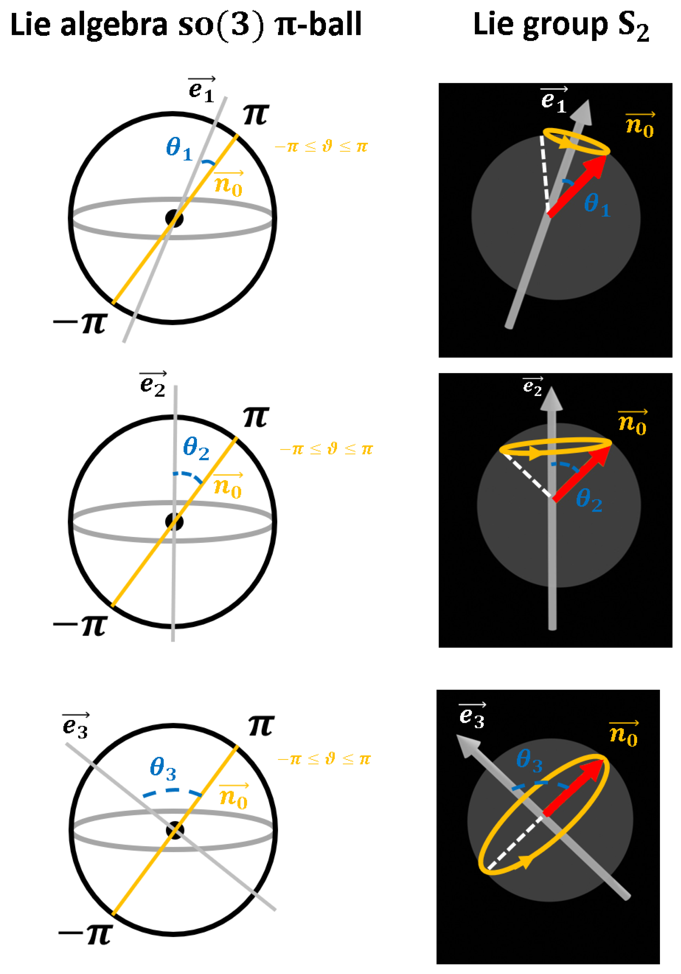
on the initial vector. As shown in Figure 1, the unit vector e defines the rotation axis. After a rotation by an angle ϑ with respect to this axis, the initial vector n 0 is mapped to
n ( ϑ ) = n 0 cos ϑ + e ( e n 0 ) ( 1 cos ( ϑ ) ) + ( e × n 0 ) sin ϑ .
Thus, the corresponding group element g ( e , ϑ ) in S O ( 3 ) is given by
g ( e , ϑ ) i k = δ i k cos ϑ + e i e k ( 1 cos ( ϑ ) ) + ϵ i j k e j sin ϑ .
On the level of the Lie algebra, we find the simple expression
g ( e , ϑ ) = exp [ ϑ e k X k ] ,
where X 1 , X 2 , X 3 are the antisymmetric generators of the Lie algebra S O ( 3 ) , given by
X 1 = 0 0 0 0 0 1 0 1 0 , X 2 = 0 0 1 0 0 0 1 0 0 , X 3 = 0 1 0 1 0 0 0 0 0 .
Obviously, the complete group can be characterized by three parameters—the direction of the rotation axis, indicated by the unit vector e with e = 1 , and the rotation angle π ϑ < π . The π -ball (with radius π ) defined by e ϑ represents all possible group elements of SO(3) on the level of the Lie algebra s o ( 3 ) . Note that the rotations ± π e are identical rotations in R 3 , therefore, antipodes of the π -ball are identified, see Figure 1 and Figure 2.
Consider the vector n 0 in R 3 . Then, the so-called o r b i t of this point is defined by g n ( 0 ) , where g runs through all group elements g ( e , ϑ ) S O ( 3 ) (that is, the full π -ball parametrizing the Lie algebra S O ( 3 ) ). Obviously, this orbit is just the unit sphere S 2 in real space R 3 . Note that there is a subset H of group elements leaving the initial vector invariant, H n ( 0 ) = n ( 0 ) . In our case, this subset is given by the rotations h ( e = n 0 , ϑ ) with π ϑ π . It is a standard result of coset theory that the coset space G / H is isomorphic to the orbit, that is,
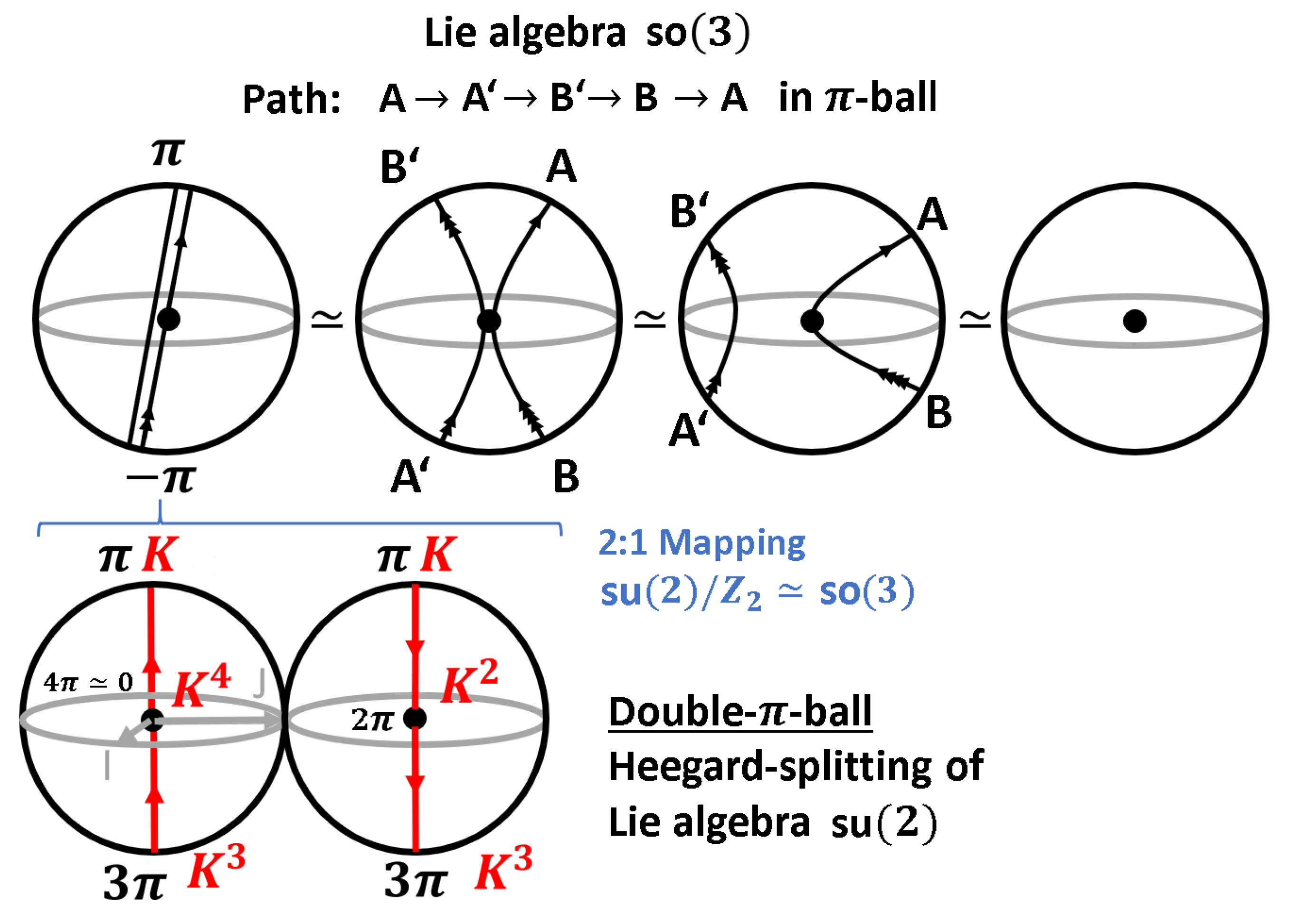
G / H = S O ( 3 ) / S O ( 2 ) S 2 .
As shown in Figure 1 and Figure 2, the rotation by 2 π around a given axis e is given by the straight line e ϑ with π ϑ < π . It is a well-known fact from group theory that this closed path is not equivalent to the Null homotopy. Indeed, as can be seen in Figure 2, only after a second traversal, the path can be deformed to the Null Homotopy (that is, to the identity element in S O ( 3 ) at the origin of the π -ball). Paul Dirac proposed a fascinating method to illustrate the corresponding motion in real space R 3 , that is, on the level of the group 
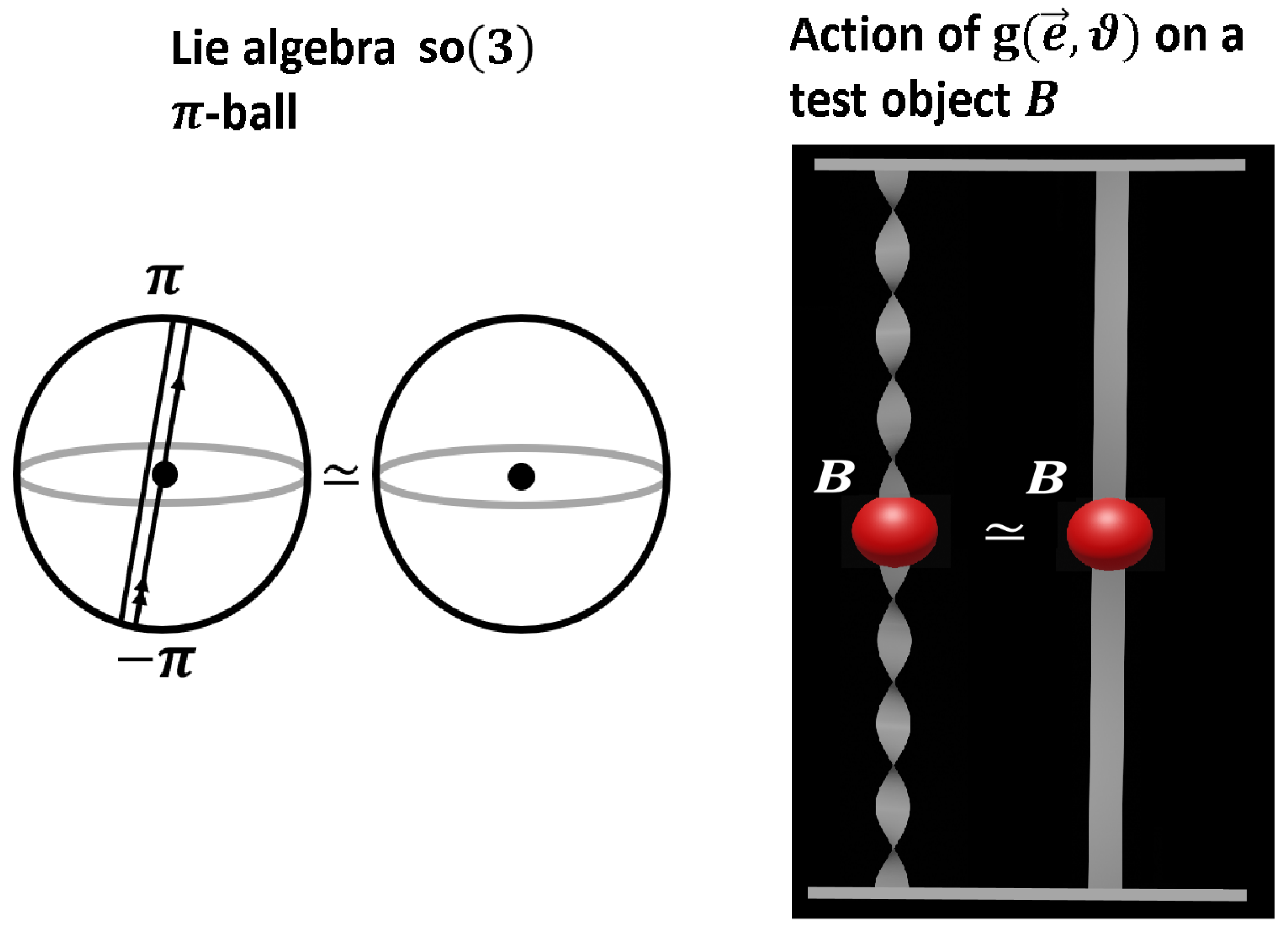
SO(3) acting on, say, a unit ball (A simulation program for the Dirac belt trick can be found in http://ariwatch.com/VS/Algorithms/Antitwister.htm). We attach this unit ball with elastic ropes (equivalently, with paper strips) to the boundary of a very large fixed outer sphere. The action of each group element 
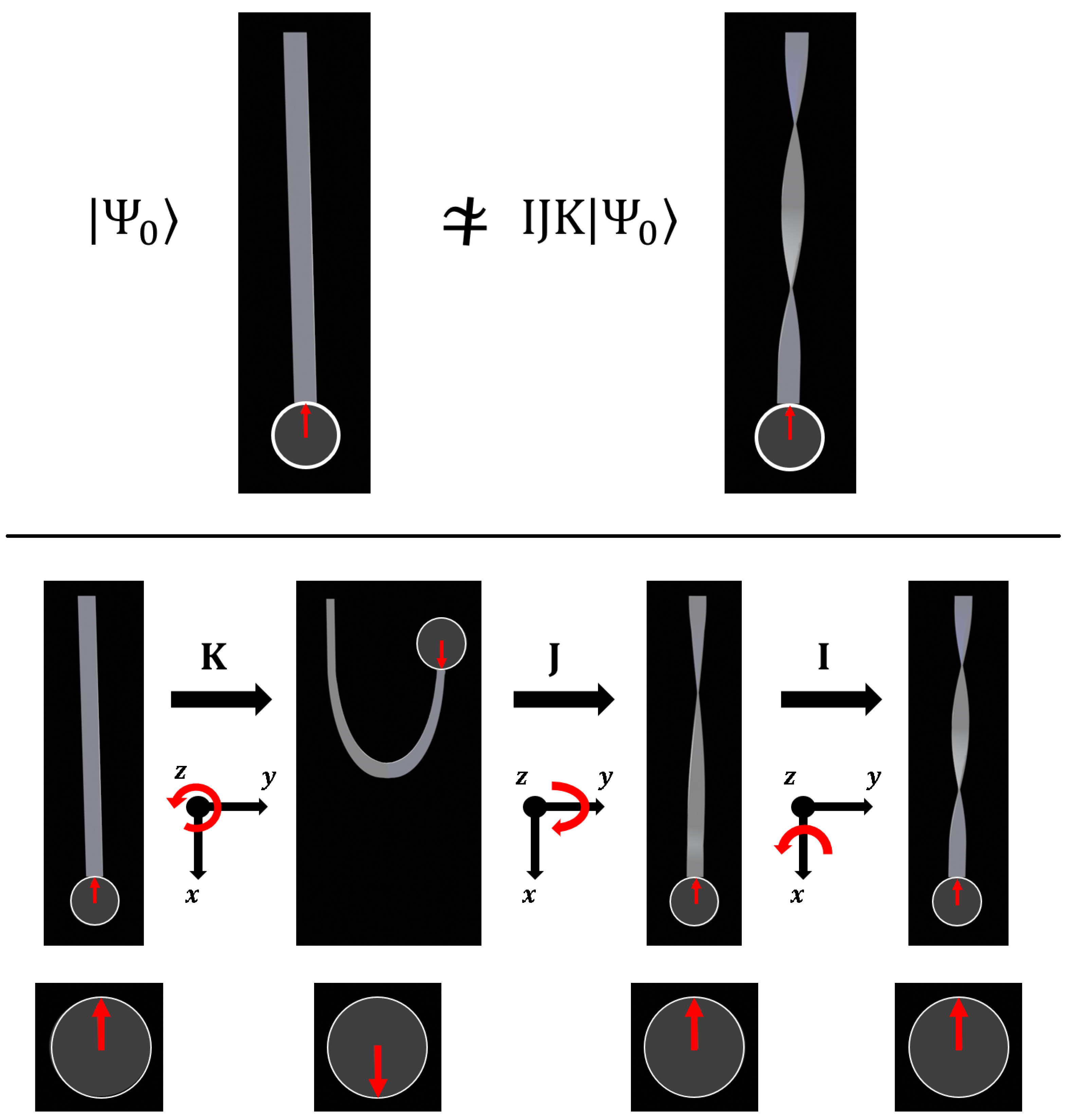
g on the unit ball is encoded in the twists of the ropes (the paper strips). As shown in Figure 3, each rotation by π can be realized as an inner t w i s t in the paper strip attached to the rotated unit ball. Indeed, it can be shown that four inner twists can be undone, but not two. This exactly corresponds to the Null Homotopy shown in Figure 2 with two traversals, that is, a ( 4 π ) -rotation (You can convince yourself of this Null homotopy: Take a paper strip and rotate it four times. You may untwist it as shown in https://vimeo.com/62228139).
The covering group of S O ( 3 ) is S U ( 2 ) , which reflects this 4 π -symmetry. The s u ( 2 ) -algebra can be constructed using the quaternions I , J , K defined by I 2 = J 2 = K 2 = 1 , and I J = K , J I = K (and cyclic). A general quaternion is given by
Q = q 0 + q 1 J + q 2 J + q 3 K ,
with Q 2 = q 0 2 + q 1 2 + q 2 2 + q 3 2 = 1 , which is geometrically just the hypersphere S 3 . The geometry of the Lie algebra s u ( 2 ) of the group S U ( 2 ) can be described by the so-called Heegard splitting—the π -ball describing the s o ( 3 ) -Lie algebra is doubled, and the boundaries of both copies of the π -ball are identified with each other. The action of I , J , K can be illustrated using the Heegard splitting as shown in Figure 2. In the covering group, 2 π and 4 π rotations can be distinguished as can also be seen in Figure 2.
Quaternions have been introduced already in the 19th century by Hamilton–much the same as the Hamiltonian for energy in classical mechanics, the full meaning of these structures became only visible more than 50 years later, with the advent of quantum physics.

3. Group Theoretic View on a Qubit in a Magnetic Field

3.1. On the Relation between SU(2) and SO(3)

As an illustrative example for the application of quaternions in quantum physics, consider the Hamilltonian
H = γ e 2 m B S ,
where describing spin precession of a qubit with spin operator S = 2 σ in a constant magnetic field B . Here, γ is the gyromagnetic factor, to be specified depending on the application, and σ x , y , z are the Pauli-matrices. The time development is given by the unitary 2 × 2 matrix
U e ( ϑ ( t ) ) = e i H t / = [ id 2 cos ( ϑ ( t ) 2 ) i e σ sin ( ϑ ( t ) 2 ) ] ,
with ϑ ( t ) / 2 = ω L t , and Larmor frequency ω L = γ e B 2 m . The unit vector e describes the direction of the magnetic field as B B e .
Next, we want to discuss this time development using group theory similar to Section 2. On the Bloch sphere S 2 , the state vector described by n rotates on a cone shell around the axis e defined by the direction of the magnetic field B = B e , as shown in Figure 1. The double cover of S U ( 2 ) can be seen explicitly by comparing Equation (1), which corresponds to the point at e ϑ in Figure 2, with Equation (4). We find
g i k ( e , ϑ ) = 1 2 tr [ U e ( ϑ ) σ i U e ( ϑ ) σ k ] ,
which just means that the two points e ϑ and ( e ϑ + 2 π ) corresponding to ± U e ( ϑ ) are separated in the two π -balls describing S 3 in the Heegard splitting as shown in Figure 2. In S O ( 3 ) , both points are identified, leading to the double cover S U ( 2 ) / Z 2 S O ( 3 ) . Both π -balls of the Heegard splitting are then merged to a single π -ball, see Figure 2.

3.2. On the Relation between Operators and Amplitudes in the Group SU(2)

Note that the Dirac belt trick, shown in Figure 3, is a priori n o quantum feature, but just a group theoretic fact about Null homotopies in S O ( 3 ) . The fundamental importance in quantum physics is due to the application of this topology to a new physical quantity introduced in quantum physics: a m p l i t u d e s arising in the wave function | ψ = u | 0 + v | 1 as complex generalizations of probabilities. Geometrically, the amplitudes ( u , v ) are also described by S 3 , since | u | 2 + | v | 2 = 1 . However, the interpretation is different - while group elements of S U ( 2 ) induce rotations, amplitudes are used to predict probabilities for observables (probability | u | 2 for the detection of | 0 , probability | v | 2 for the detection of | 1 ). In what follows, we will exploit the geometric meaning of amplitudes in more detail. We start with the orbit of the simplest possible amplitude ( 1 , 0 ) , given by
W = ( u v ¯ v u ¯ ) , orbit : W ( 1 0 ) = ( u v ) .
Note that det W = 1 . The only group element with h ( 1 , 0 ) = h is the identity, thus G / H = G S 3 , leading to an isomorphism between group elements g and amplitudes ( u , v ) . Explicitly, we can map the eigenstates ( 1 , 0 ) (or ( 0 , 1 ) ) of the rotation operator e i ϑ 2 σ z to group elements in S U ( 2 ) as
( W e i ϑ 2 σ z W ) ( u v ) = e + i ϑ / 2 ( u v ) .
The rotation axis is then transformed from the z-axis ( 1 , 0 , 0 ) to the axis n = ( n x , n y , n z ) , since
h W W e i ϑ 2 σ z W = e i ϑ 2 W σ z W = e i ϑ 2 n σ .
This rotation axis of the group element is just the direction of spin described by the amplitude ( u , v ) . This can be seen explicitly using the Hopf mapping S 3 S 2
( u , v ) n ( Re ( 2 u ¯ v ) , Im ( 2 u ¯ v ) , | u | 2 | v | 2 ) .
The vector n indicates the position where the amplitude of the state is maximal. The antipode n indicates the nodal point of | ψ = u | 0 + v | 1 on the Bloch sphere. Indeed, the state | ψ orth = v ¯ | 0 + u ¯ | 1 orthogonal to | ψ has maximal amplitude at n . In contrast to S O ( 3 ) , a rotation with angle ϑ of the state | ψ around the axis given by the vector n 0 given by (9) leads to the phase change e ± i ϑ / 2 ( e i ± ϑ / 2 ). The isomorphism between group elements and amplitudes is then explicitly
h W ( u , v ) , h W ( v ¯ , u ¯ ) .
Similar to the example shown in Figure 3, only after a 4 π -rotation, the original state is reached again.
In view of the symmetry of the hypersphere S 3 , note that there is another way to define this isomorphism, given by
h W ( v ¯ , u ¯ ) , h W ( u , v ) .
Due to symmetry, there is no physical reason to decide which isomorphism should be used.
Each group element h W is defined by three parameters ϑ 2 n with 0 ϑ 4 π . A priori, these parameters have no physical interpretation. It depends on the context, whether the parameters in the corresponding state | ψ = u | 0 + v | 1 play the role of time development, or of a (space-like) angle in S 2 , or just of an irrelevant phase. In the explicit parameterization
u = e i ϑ 2 i ϕ 2 cos [ θ 2 ]
v = e i ϑ 2 + i ϕ 2 sin [ θ 2 ] ,
where we find that each phase 0 ϑ = ω L t < 4 π maps to one specific group element h U in case that | ψ is an eigenstate of H , that is, for B = B n . On the Bloch sphere, the equivalence class of states | ψ ( ϑ ) = u | 0 + v | 1 for any ϑ is represented by the single vector n = ( cos ( θ ) , sin ( θ ) cos ( ϕ ) , sin ( θ ) sin ( ϕ ) ) as shown in Figure 4.
Note that h W , h W are the only operations which only change a global phase of the state ( u , v ) . For fixed n , this is a U ( 1 ) -subgroup within S U ( 2 ) . All other rotations U e ( ϑ ( t ) ) as defined in (4) with axis e n change the position of the direction of maximal amplitude, that is, lead to spin precession, as shown in Figure 1 on the Bloch sphere S 2 . We conclude that S U ( 2 ) / U ( 1 ) S 2 .

3.3. Spin Flip Operations in a Generalized Bloch Sphere Representation

In this section, we introduce an important class of unitary operations on qubits, the so-called spin-flip operations. It turns out that the usual Bloch sphere representation will be insufficient for our purpose, as sign changes in the amplitude of the wave function upon 2 π -rotation cannot be displayed on the Bloch-sphere. For this reason, a knot theoretic model in Hilbert space (in this case, S 3 ) will be introduced, inspired by the Dirac belt trick.
Spin-flip operations with ϑ = π as in Equation (4) are of special importance in many applications, for example, in quantum computation. A basis of spin-flips is given by rotations in x , y and z-directions. For spin j = 1 / 2 , spin flips are described by the q u a t e r n i o n s I , J , K as
I exp ( i π 2 σ x ) = i σ x J exp ( i π 2 σ y ) = i σ y K exp ( i π 2 σ z ) = i σ z .
The homotopy I J K = J K I = K I J = e ( 2 π i ) / 2 = 1 connects the identity operation with negative identity, as shown in Figure 5, which is different from the Null homotopy I K J = + 1 . However, this sign change is not visible in the Bloch-sphere representation, since both π -balls representing S U ( 2 ) are identified and mapped to the boundary S 2 in the Bloch sphere representation. We conclude that albeit the Bloch-sphere representation is of immense importance in practice, it does not describe the full dynamics in Hilbert space, since S U ( 2 ) / U ( 1 ) S 2 is ( 2 π ) -periodic.
However, similar to Figure 3, we can track the motion of the Bloch sphere by attaching (elastic) paper strips. It is sufficient to attach just one paper strip at the position of maximal amplitude as shown in Figure 6. Then, each rotation of the Bloch sphere is tracked, and the difference between a ( 2 π ) -rotation (corresponding to two inner twists in the paper strip) and a ( 4 π ) -rotation (corresponding to four inner twists, which can be undone by the Dirac belt trick) becomes obvious. As shown in Figure 6, any motion of the Bloch sphere can be tracked using the three basic spin flip operations I , J , K .
Note that ’open’ paper strips (linking the Bloch sphere to an infinitely large outer ball) track all unitary rotations acting on any quantum state defined on the Bloch sphere. As unitary operations define time development in quantum physics, the model proposed in Figure 6 combines a ( 4 π ) -representation for time development with a ( 2 π ) -representation of the quantum state on the Bloch sphere. By replacing the spin j = 1 / 2 state by any other spin j-state on the Bloch sphere, this model can be generalized to any spin.
In the next section, we replace the ( 2 π ) -representation for the quantum state on the Bloch-sphere by the ( 4 π ) -representation, which is related to c l o s e d paper strips modeling torus knots in Hilbert space. In other words, we describe the quantum state in S 3 , and not after the Hopf-mapping S 3 S 2 .

3.4. Modeling Amplitudes with Closed Paper Strips

We discuss the amplitude of the state | 0 at position | ψ ( | ψ orth ). We find
| 0 = | ψ ψ | 0 + | ψ orth ψ orth | 0 = u | ψ v ¯ | ψ orth .
A global rotation with the corresponding eigenoperator of | 0 leads to
e i ϑ 2 σ z | 0 = u e i ϑ 2 σ z | ψ v ¯ e i ϑ 2 σ z | ψ orth .
Starting with the equivalence class of states
| ψ = e + i τ 2 ( cos ( θ / 2 ) , sin ( θ / 2 ) ) ,
where we find for the homotopy λ e i ϑ 2 σ z | ψ , weighted with amplitude λ = u
λ e i ϑ 2 σ z | ψ = λ ( e + i τ ϑ 2 cos ( θ / 2 ) , e + i τ + ϑ 2 sin ( θ / 2 ) ) λ ( X + i Y , U + i W ) ,
with X 2 + Y 2 + U 2 + W 2 = 1 . As shown in Reference [4], for fixed θ , we obtain a bundle of ( 1 , 2 ) -torus knots, that is, a Dirac belt. For simplicity, we choose the torus at θ = π / 2 , that is, we consider
( X + i Y , U + i W ) = ( 1 2 e + i τ ϑ 2 , 1 2 e + i τ + ϑ 2 ) .
Using stereographic projection as
( X , Y , U , W ) ( X 1 W , Y 1 W , U 1 W ) ,
where we obtain a visualization of the invariant torus with respect to the spin-rotation operator K as shown in Figure 7. Note that this projection is just done in order to be able to make a plot of the complex geometry in three dimensions. It is no surprise to find torus knots in the geometry of S 3 [5,6]. Indeed, spin j representations are related to ( 2 j , 2 ) torus knots, which can be represented using the paper strip model generalizing the Dirac belt to spin j [4]. In Appendix A, we briefly review this generalization. In the Bloch sphere representation, only the position n of maximal amplitude ( λ = 1 ) is shown. However, in Hilbert space S 3 , at any position an amplitude emerges as shown in Equation (16) with λ = u at the point | ψ ( λ = v ¯ for | ψ orth ). In general, any given quantum state is defined by a m p l i t u d e s   0 | λ | 1 which ’excite’ certain Dirac belts. In other words, the presence of ( 2 j , 2 ) torus knots is just a geometric feature of S 3 , and it is the pattern of amplitudes within S 3 which characterizes the quantum state. Similar to the excitation of piano strings, the changing amplitudes in what we call ’time’ describe the ’quantum melody’ of unitary time development.
As shown in Figure 7, the Dirac belt with four inner twists is mapped to a Möbius strip with one twist after gluing together the two pieces ( 0 , 2 π ) and ( 2 π , 4 π ) of the Dirac belt [4]. This describes the 2:1 Hopf-mapping from the ( 4 π ) -realm, that is, the Hilbert space, to the ( 2 π ) -realm, that is, observables.
In general, the phase e i j ϕ on the equator of the Bloch sphere is related to 2 j twists in the ( 2 π ) -realm, which in the paper strip model in the ( 4 π ) -realm lead to ( 2 j , 2 ) torus knots with 4 j + 2 inner twists for fermions (j half-integer), and 2 l × 2 l inner twists for bosons ( j = l integer) [2]. As shown in Reference [7], the exchange of two particles is homotopically equivalent to a ( 2 π ) -rotation of one of these particles. Note, that in two dimensions, anyons with any phase upon exchange of two particles may arise. A ( 2 π ) -rotation leads to the phase change e 2 π i j , which is the clue to the bosonic and fermionic statistics upon exchange of particles.

4. Paper Strip Model Model for a Pair of Entangled Qubits

Operations on two qubits are described by the unitary group U ( 2 2 ) = U ( 4 ) . Due to symmetry, all points in S U ( 4 ) are equivalent from a geometric point of view. It is the Hamiltonian which creates certain interpretation patterns within this geometry. For a given Hamiltonian, we can define a basis { | 00 , | 01 , | 10 , | 11 } of pairs of qubits. Pure states are described by the orbit of | 00 , that is, the hypersphere S 7 . While product states are only the small subsection S 3 × S 3 within S 7 
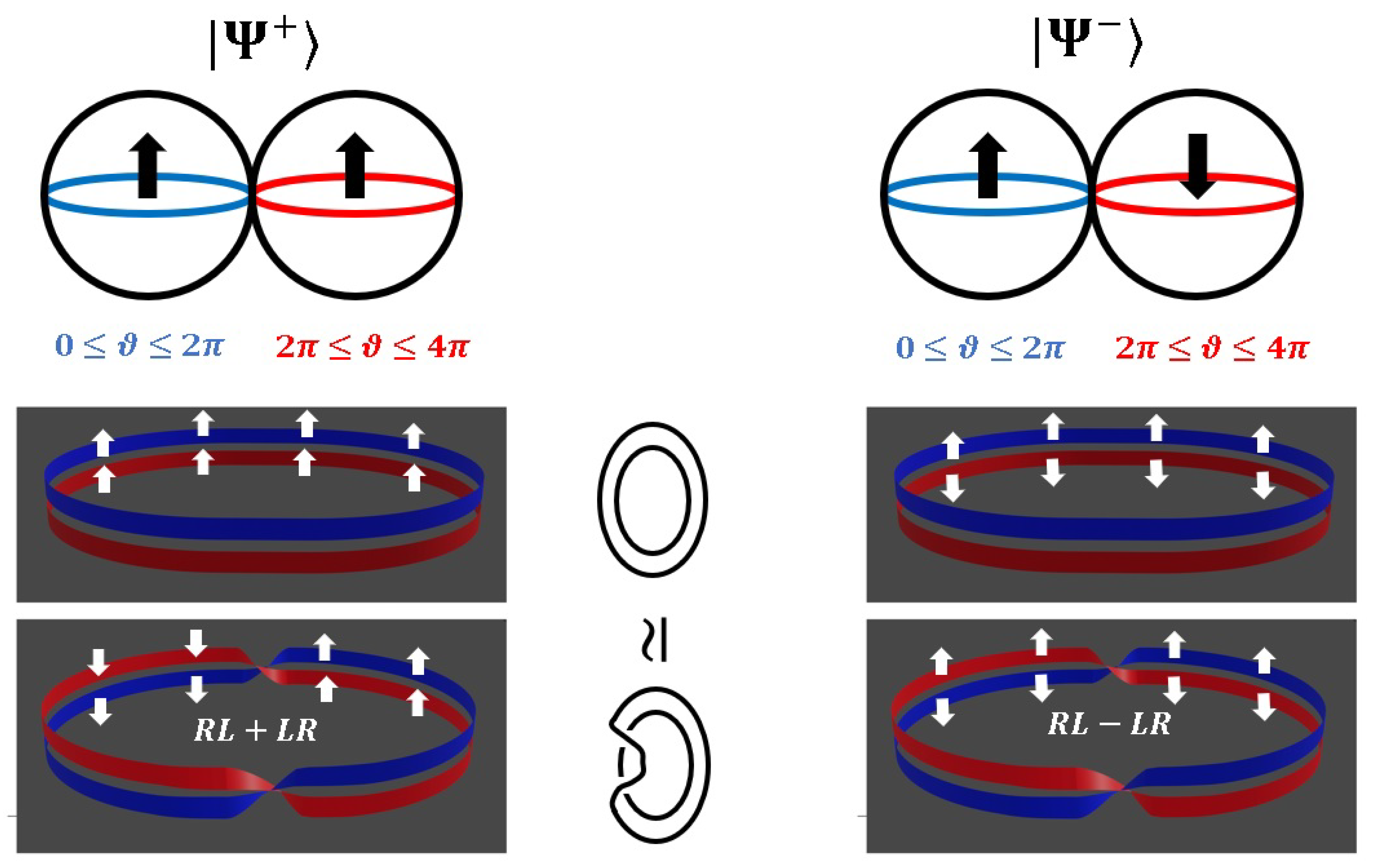
, all other states are (partially) entangled. The Bell-states represent maximally entangled states. We discuss the Bell states
| Ψ + = 1 2 ( | 01 + | 10 ) = 1 2 ( | + + | ) | Ψ = 1 2 ( | 01 | 10 ) = 1 2 ( | + | + ) .
While | Ψ + is part of the spin triplet with j = 1 , | Ψ is the antisymmetric spin singlet state with j = 0 , which is basis invariant. As discussed in detail in Reference [3], for any maximally entangled state, there exists a homotopic loop where the amplitude of | Ψ + remains constant. For | Ψ + , this is the rotation in z-direction
| Ψ + = 1 2 ( | 01 + | 10 ) = ( e i ϑ 2 σ z × e i ϑ 2 σ z ) 1 2 ( | 01 + | 10 ) .
Thus, the amplitude upon the z rotation remains constant, since λ z = Ψ + | ( e i ϑ 2 σ z × e i ϑ 2 σ z ) Ψ + = 1 In contrast, the rotation in x-direction leads to
| Ψ + = 1 2 ( | + + | ) = ( e i ϑ 2 σ x × e i ϑ 2 σ x ) 1 2 ( | + + | ) = 1 2 ( e + i ϑ | + + e i ϑ | ) .
Thus, the amplitude upon the x rotation is given by λ x = Ψ + | e i ϑ 2 σ x × e i ϑ 2 σ x Ψ + = cos ( 2 ϑ ) . As discussed in the previous section, these amplitudes have infinitely many topologically equivalent representations. The paper strip model is one possible method to display these configurations, as shown in Figure 8.
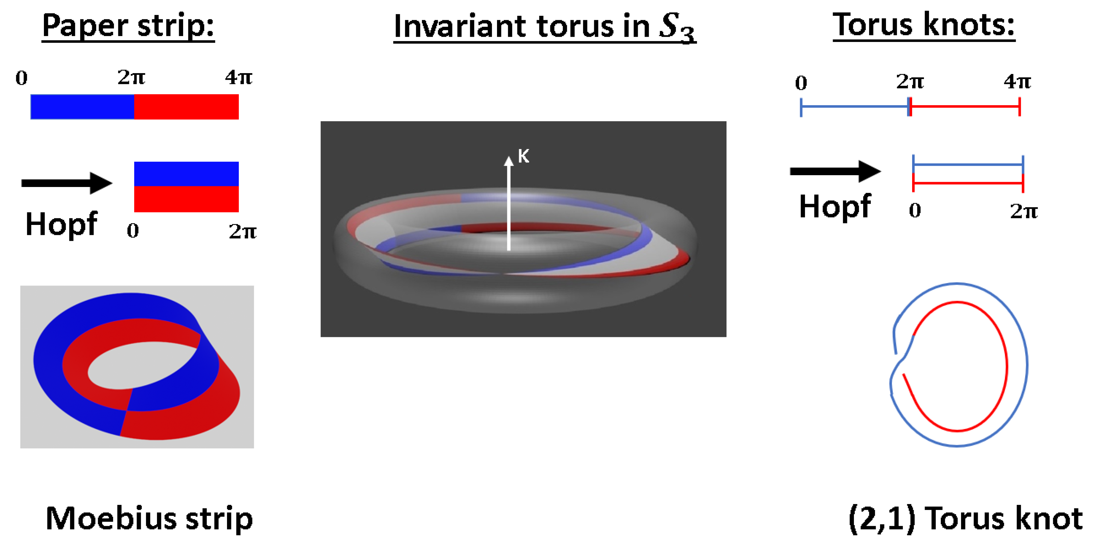
One merit of the paper strip model is the possibility to visualize topologically equivalent configurations which represent the same quantum state, or to be more precise, the same amplitude on a certain homotopic loop in Hilbert space. We discuss the homotopic loop with constant amplitude, because this provides a nice representation for entanglement—as discussed in detail in Reference [3], this constant phase is topologically equivalent to a combination of one right twist R and one left twist L (see Figure 9).
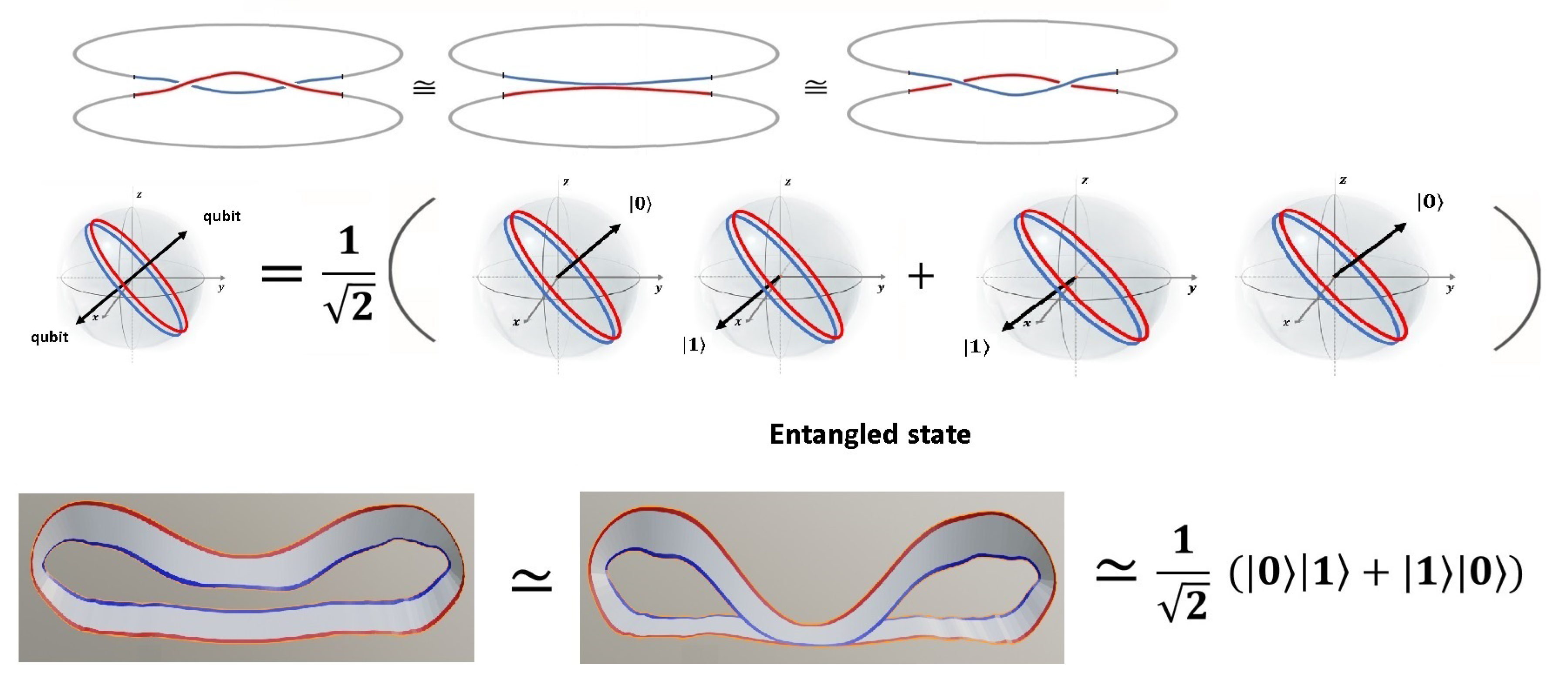
In other words, the quantum phase of the Bell state | Ψ + is much less complicated as it seems—the states | 0 and | 1 merge to a constant phase, as their individual properties vanish. Thus, due to our choice to express the entangled state in the basis | 0 , | 1 , it is necessary to symmetrize and to write the complicated expression 1 2 ( | 01 + | 10 ) as shown in Figure 10.
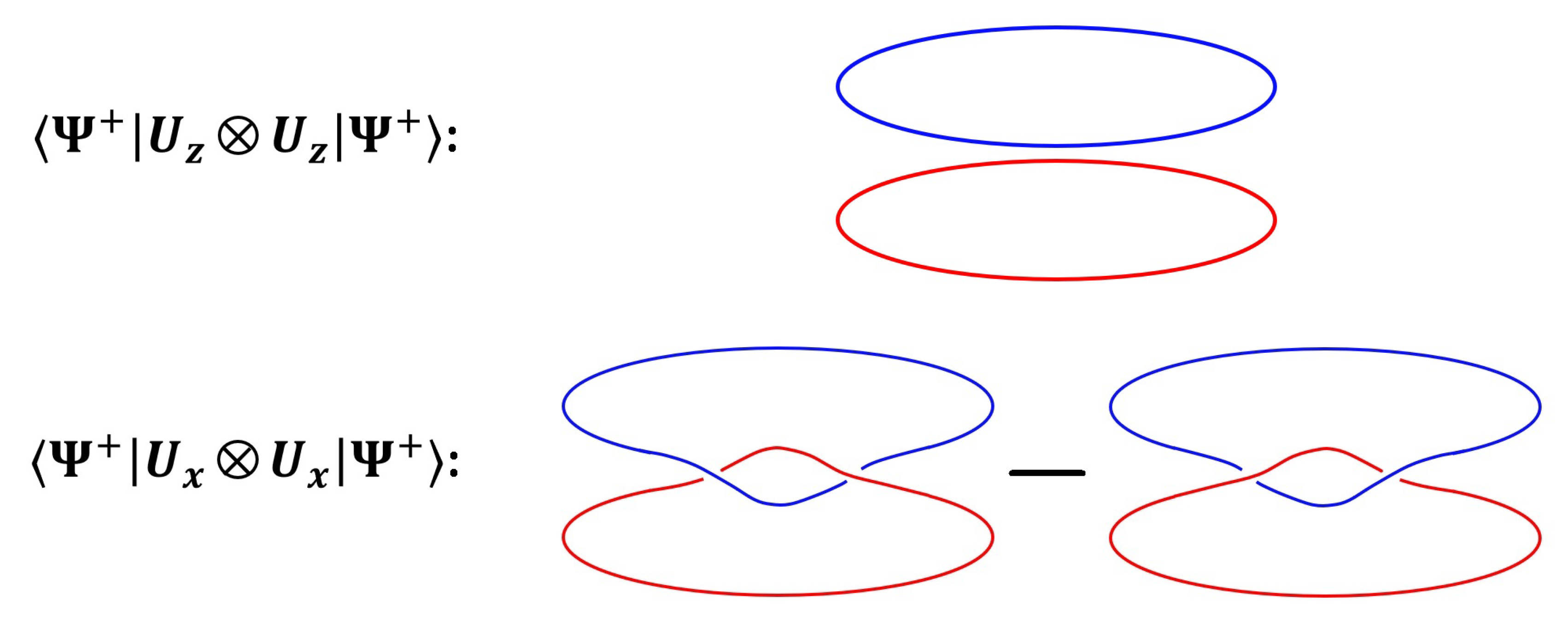
As the singlet state | Ψ remains invariant under any rotation, the amplitude is constant on every homotopic loop, as expected for the state with a total spin of zero. Due to antisymmetry, the amplitude must vanish, and | Ψ is a pseudo-scalar. The exchange of both ’particles’ of the entangled state amounts to a rotation of 2 π which can be done just by exchanging the role of both π -balls in the Heegard splitting. Indeed, as shown in Figure 9, this leads to a global minus sign in case of | Ψ .

5. Kochen-Specker Theorem

As a first application of the knot theoretic extension the Bloch sphere representation of qubits, we discuss the Kochen-Specker theorem, which states that noncontextual hidden-variable theories are incompatible with predictions of quantum theory [8]. We denote by q ( A ) , q ( B ) the eigenvalues related to the operators A and B. For a set of commuting observables, noncontextuality implies that the values of the observables are independent of the context, that is, independent of the other commuting observables. In particular, this means q ( A B ) = q ( A ) q ( B ) . This assumption contradicts quantum physics, as was first shown by Kochen and Specker [9]. While the first proof involved 117 vectors in four dimensions, Peres found a much simpler proof with nine observables in four dimensions in a system of two qubits [10]. Later, Mermin [8] introduced a set of observables known as Mermin’s square, and proposed a state-independent proof.
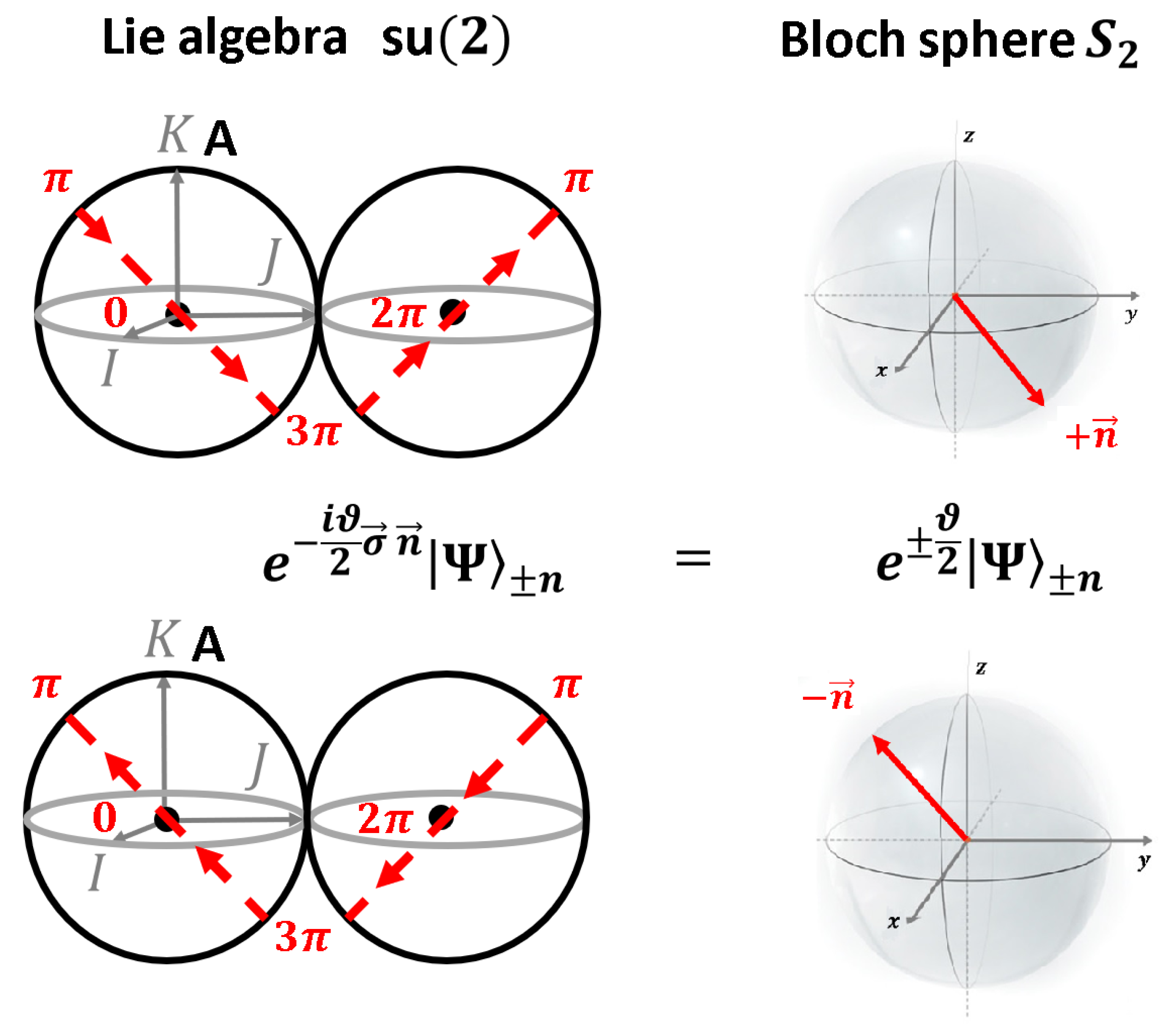
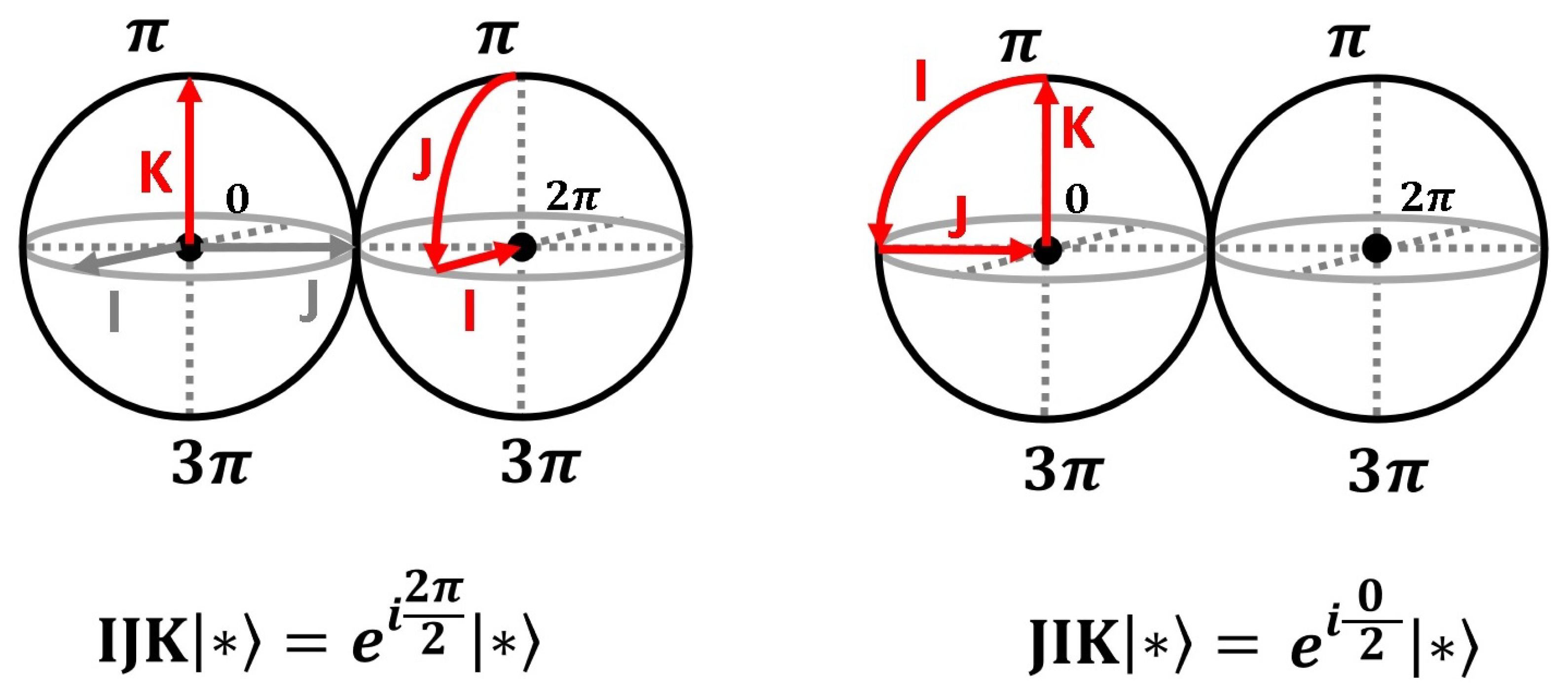
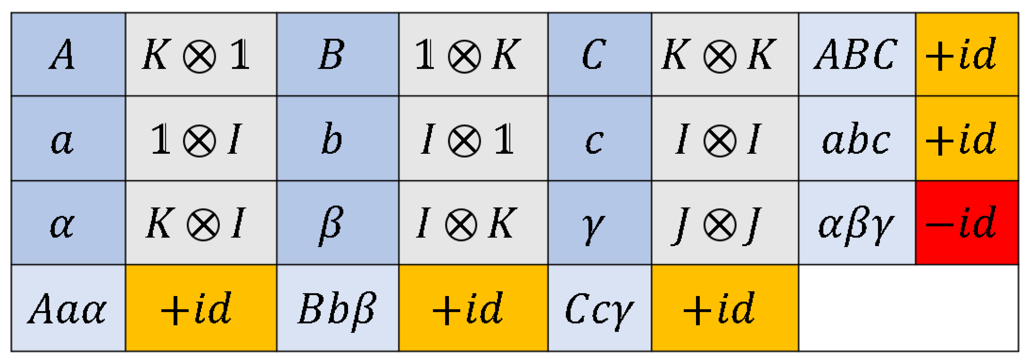
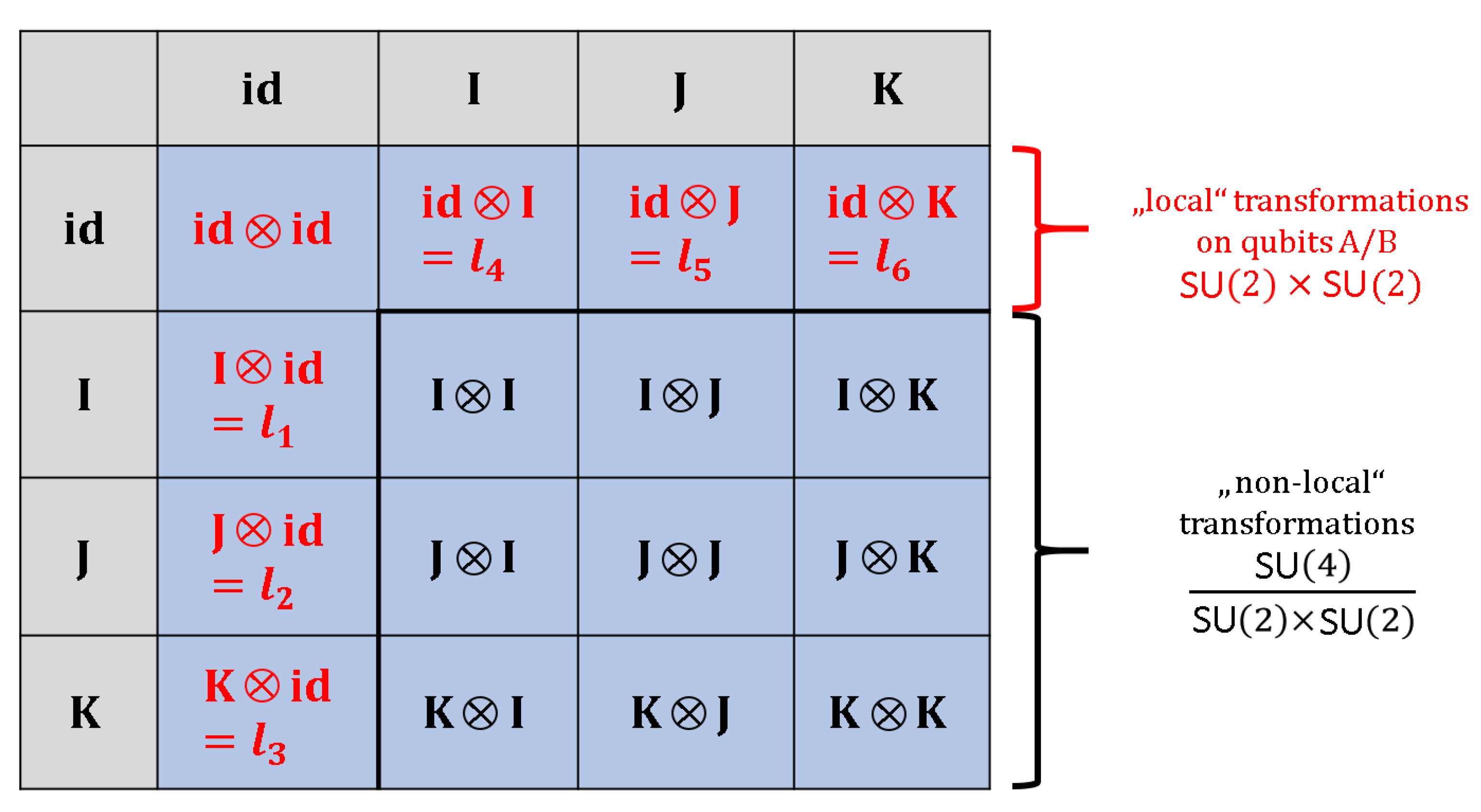
Following Peres and Mermin, we consider a combination of spin-flip operations Q 1 × Q 2 acting on a system of two qubits, as shown in Figure 11. Indeed, in each row and each column, the observables mutually commute, and can be measured simultaneously. On the level of the spin-flip operators, the product of all rows and columns is given by
( A a α ) ( B b β ) ( C c γ ) ( A B C ) ( a b c ) ( α β γ ) = id 5 ( id ) = id .
Note that this result crucially relies on the difference between the paths I J K = 1 and J I K = + 1 , as shown in Figure 5 on the level of the Lie algebra. The action on a given the quantum state by the corresponding group element in SU(2) is shown in Figure 6. Concerning the eigenvalues, the assumption of noncontextuality translates to the statement that the eigenvalues ± i of each spin-flip operator I , J , K (14) would be independent of the context. This implies that the product of eigenvalues of all rows and columns is independent of the combination of other observables involved, that is,
p ( A a α ) p ( B b β ) p ( C c γ ) p ( A B C ) p ( a b c ) p ( α β γ ) = p ( A ) 2 p ( a ) 2 p ( α ) 2 p ( B ) 2 p ( b ) 2 p ( β ) 2 p ( C ) 2 p ( c ) 2 p ( γ ) 2 = + 1 .
Obviously, the assumption of noncontextuality contradicts the result for the operators (24).
Several experiments revealed that the assumption of noncontextuality is in contradiction with observation. The Kochen-Specker-Theorem applies to all systems with three or more levels. While using so-called qutrits as a basis of experimental tests is possible, the use of four level systems seems to be the more widely applied method. A four-level system can easily be created by joint measurement of two qubits, regardless whether the two qubits are realised across different particles or as different degrees of freedom within a single quantum object. An illustrative example for a testing scheme using single photons is provided by Reference [11], where a polarizing beam splitter is used to associate polarization (labelled superscript ’p’ with vectors H / V for horizontal and vertical polarization) and spatial path information (labelled superscript ’s’ with vectors t , r for transmission and reflection). By implementation of additional rotation and phase shift operations, arbitrary states can be generated within these two degrees of freedom.
As shown in Figure 11, it is straightforward to show for an appropriate set of observables that the quantum mechanical prediction is at odds with the idea that each of the observables has a predefined value of +1 or −1 before measurement. In terms of expectation values obtained by measurements on statistic ensembles, the contradiction shown in Equations (24) and (26) can be brought into the form of an inequality which gives a criterion for experimental testing of contextuality [12]. Under the assumption of noncontextuality, the measured expectation values can be expected to obey the following relation:
χ = A B C + a b c α β γ + A a α + B b β + C c γ 4
while quantum physics as a contextual theory predicts an outcome of χ = 6 (see Figure 11). The experimental task is therefore to find a suitable sequence of polarization and spatial path measurements, that is, of some combinations of the observables σ x , y , z p and σ x , y z s that correspond to the nine operators in Equation (26).
It is important to note that even though the concrete choice of combinations of observables leading to a contradiction might vary with the details of the experimental implementation, Equation (26) is not dependent on any specific features of the quantum state it is applied to, hence it provides a powerful tool for testing contextuality in a very broad range of cases and applicable to entangled states as well as product states and even mixed states of four level systems [13].
Since the first experimental tests for contextuality had been undertaken in the early 2000’s, different variations of inequalities have been tested in different experimental settings, using various physical substrates to implement three- or four-level systems. The range of implementations includes photonic states [13,14,15,16,17], but also trapped ions [18], free neutrons [11] and molecular nucelar spins in the solid state [19]. Some of these tests rely on inequalities that are explicitly restricted to specific classes of states [11,15,16,17], while some experimental settings also allow for testing of state-independent inequalities like Equation (26), providing experimental evidence of contextuality for a broad range of states [13,14,18]. Even technological applications based on quantum contextuality have been discussed, for example the prospect for new methods in cryptography [20] or models of quantum computing based on contextuality [21].
In a nutshell, the Kochen-Specker theorem is an interesting variant to the fact that Hilbert space relies on a ( 4 π ) -symmetry rather that a ( 2 π ) -symmetry, which has already been shown long before with neutron interferometry of a simple single qubit in a magnetic field with a Hamiltonian similar to that discussed in Section 3 [22,23]—here, it was shown for the first time experimentally that 2 π -rotations differ from 4 π -rotations. Thus, experiments give strong hints that the Hopf mapping between ( 2 π ) -rotations and ( 4 π ) -rotations is not just a mathematical curiosity of 19th century mathematics, but lies at the heart of the quantum nature of the observable universe.
Using this geometric point of view, noncontextuality can also be interpreted as follows: As shown in Figure 5, the path of the quaternions
h ± ( ϑ ) = e ± i ϑ 2 σ n ,
where in the Lie group S U ( 2 ) is just a straight line in the Heegard splitting. The sign ± just changes the direction of the motion along that path. Traversing the Dirac belt in reverse direction, the role of ’left’ and ’right’ twists is exchanged. But is there a way to distinguish left-moving from right-moving on a microspoic scale? In other words, is there a possibility to refer to a convention (a context) to assign ’left’ and ’right’? On the level of the relation between amplitudes and operators, as already seen in Equations (10) and (11), the definition of the sign is a r b i t a r y due to symmetry. Only a relative sign, that is in the context of a given convention, can be defined.
On the level of the paper strip model, suppose you have a Möbius strip (equivalently, a Dirac belt in the ( 4 π ) -realm) at your disposal in a completely empty space, without any reference frame. There would be no way to assign a l e f t - or a r i g h t - twist to this Moebius strip (the same is true, of course, for inner twists of the Dirac belt). Only by comparing this Moebius strip to a second one, it would be possible to decide whether both are tilted the same way, or in the opposite way. We conclude that as long as parity symmetry is not violated, a priori, there is no way to define ’ left’ and ’right’ in a unique manner.

6. Many-Worlds Theories of Quantum Physics

As second application of the knot theoretic extension of the Bloch sphere representation of qubits, we discuss many-worlds theories.
The original idea by Hugh Everett [24] of a quantum physics without collapse of the wave function has been published under the title “Relative State Formulation of Quantum Mechanics” in 1957. Only later on, the compelling title “Many-worlds interpretation” was invented by DeWitt, making this approach more popular since the late 1960s [25]. Albeit of no practical importance, up to today, the theory attracts much interest and plays an important role in the debate concerning the interpretation of quantum physics [26]. Even after more than sixty years, there is no generally agreed set of postulates defining ’the Everett interpretation of quantum theory’, rather, there are ’many worlds’ in the interpretation of the many-worlds theory itself. In any case, the key idea of many-worlds theories is to consider unitary evolution as sufficient for the description of quantum physics and to avoid the necessity of a ’collapse’ of the wave function. For example, Carroll states that the many-worlds theory is the most straightforward approach to quantum mechanics [27]: There is only the unitary group in quantum physics, with all possible wave functions at disposal. When something is realized in our world, the other possibilities contained in the wave function do not vanish. Instead, according to many-worlds theories, new worlds are created, that is, each possibility is a reality.
Interestingly, the paper strip model provides a simple argument a g a i n s t 
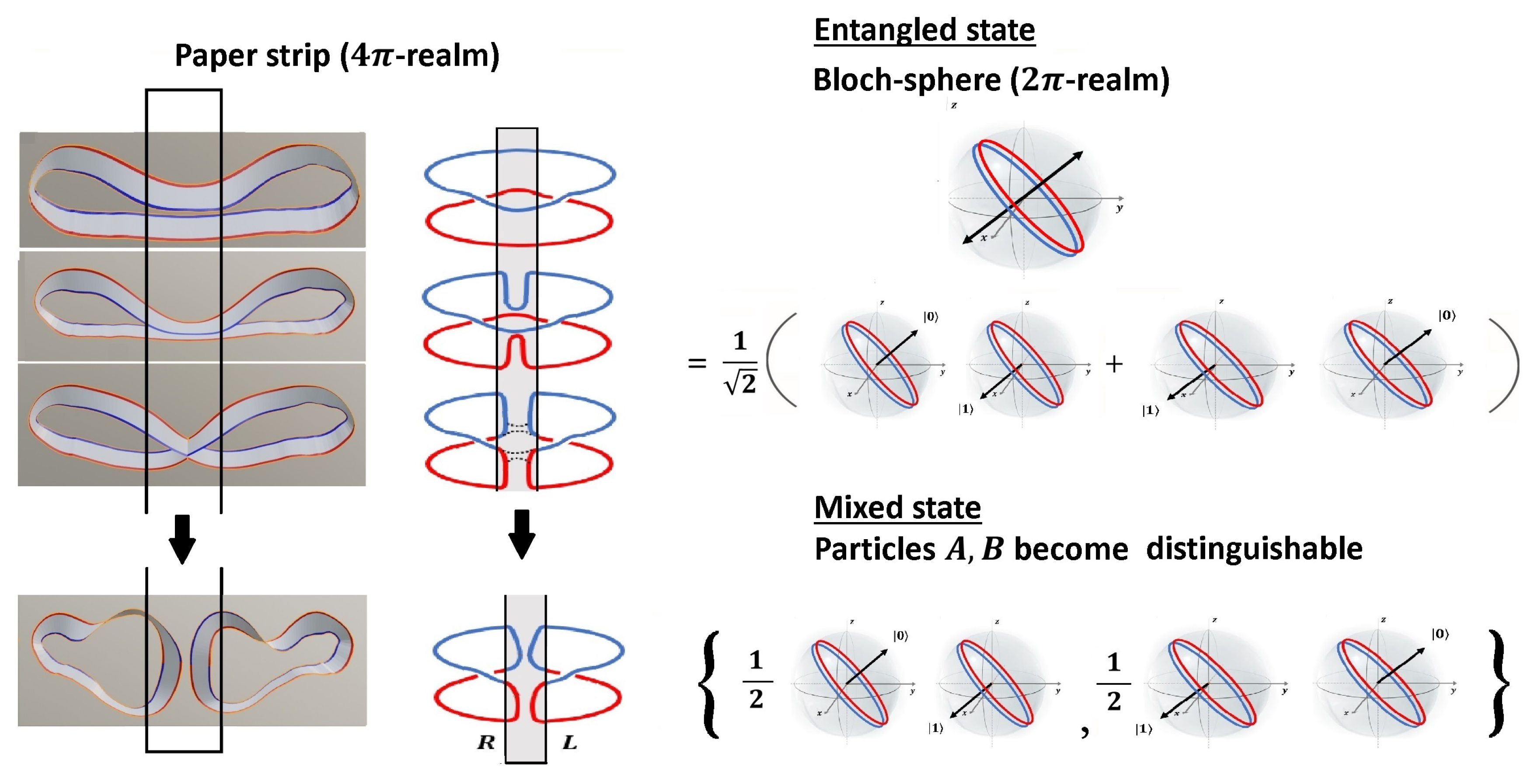
many-world theories, using the very same argument that only the symmetries of the unitary group are at disposal. Suppose that the interaction between two qubits causes entanglement. As a n y kind of interaction causes entanglement, this is a reasonable assumption to start with. Consider the entangled state
| Ψ + = 1 2 ( | 0 A | 1 B + | 1 A | 0 B ) ,
where in a given basis set ( | 0 , | 1 ) . The transition from the entangled state to a mixed state can easily be modeled as decoherence due to coupling to an environment of many qubits [28]. The result is the transition of the entangled state to a mixed state. In any case, measurement leads to the transition into a state where the states | 0 | and | 1 become distinguishable.
Many-worlds theory claims that once we measure the state | 0 at A (Alice) and | 1 at B (Bob), this implies that the ’other’ part of the wave function ( | 1 at A and | 0 at B) is realized in a parallel universe. However, as shown in Figure 12, in our description there is no ’other part’ of the wave function. Rather, the labels A , B are meaningless for an entangled state, as all individual properties of these particles disappear in the state | Ψ + . In (28), the superposition of product states is needed to wash out the significance of the labels A , B , that is, to u n d o the possibility of two ’parts’ of the wave function. Indeed, the entangled state can be represented just as a constant phase, which is topologically equivalent to the combination of two opposite twists [3]. It is impossible to uniquely label A and B to these twists, as all homotopically equivalent variants coexist, as shown in Figure 10. The same result comes from the fact that the choice of sign of the homotopy in (23) is arbitrary, thus without context. The definition of R and L twist is arbitrary. If for some reason, for example, due to decoherence, two distinguishable particles A, B emerge, it is obvious from Figure 12 that only a s i n g l e p a i r | 0 , | 1 of qubits can be produced from the original entangled state. What is not yet determined is the labeling A, B for the pair | 0 , | 1 . In other words, the context where the states | 0 , | 1 emerge is not determined. But i f the eigenvalue of | 0 is defined + 1 in the context A, then it must be 1 for | 1 in B. Since this labeling is arbitrary at first, with probability p = 1 / 2 the labeling is either | 0 A | 1 B or | 0 B | 1 A . This is just the transition from the entangled state to the mixed state shown in Figure 12, formally given by
| Ψ + Ψ + | 1 2 [ | 0 A 1 B 0 A 1 B | + | 1 A 0 B 1 A 0 B | ] .
Due to this transition, the off-diagonal terms of the density matrix vanish, indicating that particles A and B become distinguishable. Once the particles A , B become distinguishable from each other, there is no ’parallel universe’ opening with the inverse combination, simply because the association of the single pair of Dirac belts representing the states | 0 , | 1 shown in Figure 12 to the qubits A , B can only be done once. We become aware of these two possibilities only if we observe many particles, since in the context of the first particle pair, we can only distinguish the sign difference. This leads to the ensemble interpretation of the wave function by only using symmetries and geometric properties of the unitary group.
More generally, we can reformulate this argument based on a g e o m e t r i c view of quantum physics [29]: In the unitary group S U ( 2 ) , there is complete symmetry between all parameters describing the group. At first, all points on the sphere S 3 are equally meaningless. The Hamiltonian (see Section 3 for an example) defines what ’time’ is within S 3 . For example, as shown in Figure 4, the direction of the magnetic field defines the parameter ’time’ in S 3 , and in turn, the interpretation of the parameters of the quantum states as time-like and space-like, as defined in (13).
In the case of S U ( 4 ) relevant for the entanglement of two qubits, the same holds true. At first, all points on the hypersphere S 7 are equally meaningless. In an arbitrary basis, we may introduce the coordinates
| ψ = z 00 | 00 + z 01 | 01 + z 10 | 10 + z 11 | 11 ,
where for a general pure state, equivalent to S U ( 4 ) / S U ( 3 ) . Within S 7 , infinitely many possibilities to define two qubits in the six-dimensional subspace S 3 × S 3 (equivalently, S U ( 2 ) × S U ( 2 ) ) coexist. We may call this S U ( 2 ) × S U ( 2 ) transformation ’local’, acting on each separate qubit alone. In terms of dimensions, within the seven dimensions from S 7 , one more ’non-local’ dimension is left. As shown in Reference [
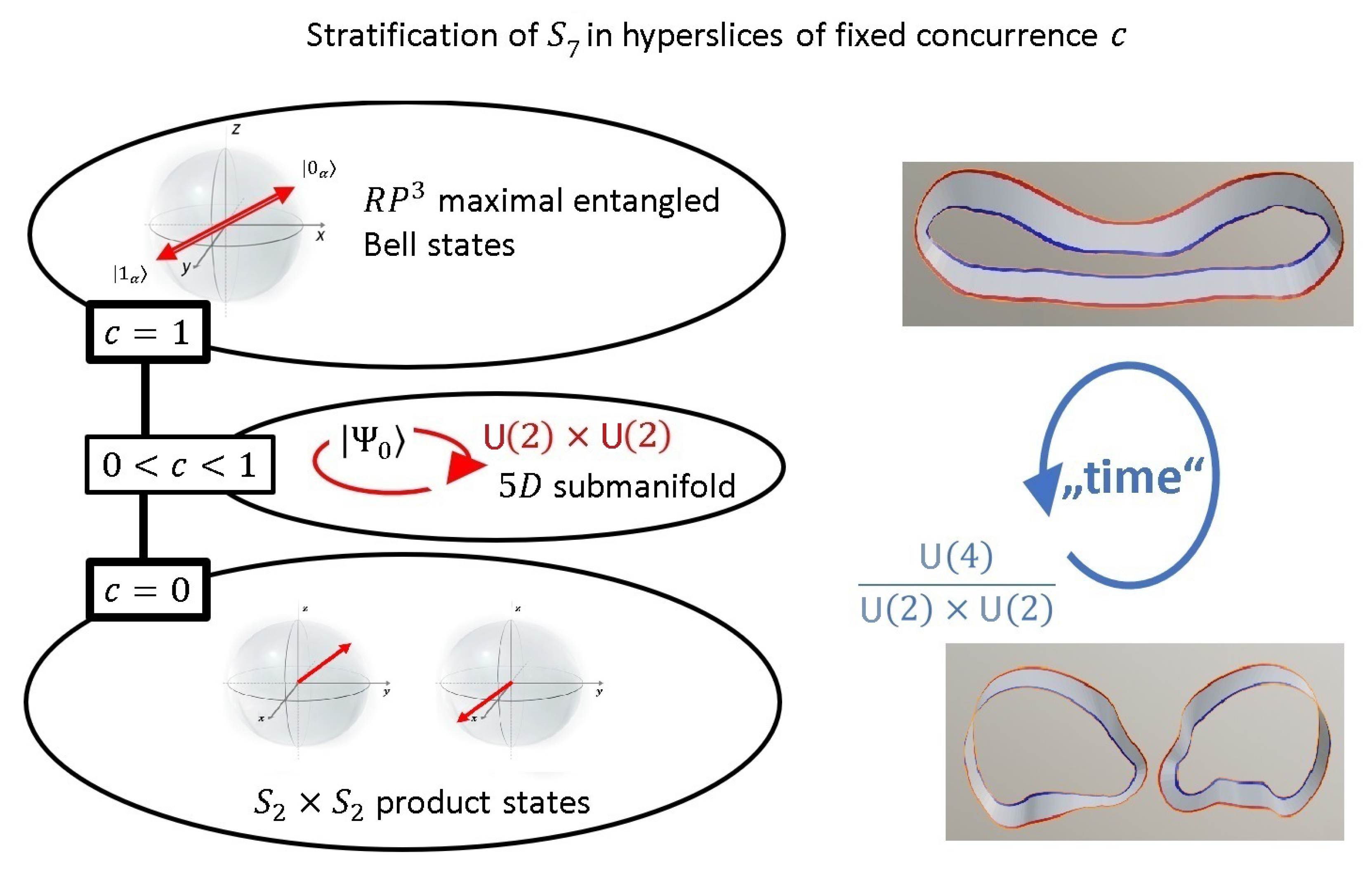
30], this dimension can be defined as concurrence c, given by
c = 2 | z 00 z 11 z 01 z 10 | .
For c = 0 , we obtain the subspace S 3 × S 3 of two independent qubits, while c = 1 defines the subspace R P 3 of maximally entangled Bell-states as shown in Figure 13. The structure of the interaction is defined by the Hamiltonian H Q i × Q j . Here, Q 1 , Q 2 are two quaternions as defined in Equation (2). It is this Hamiltonian which defines what is ’time’ within S 7 . As interaction leads to entanglement, indeed, the concurrence c is intimately related to time development in case of interaction.
The time development with the unitary matrix exp [ i H t ] S U ( 4 ) / ( S U ( 2 ) × S U ( 2 ) ) leads to an oscillation between the states of separate qubits with c = 0 , and maximally entangled states with c = 1 [28]. The ’local’ unitary operations S U ( 2 ) A × S U ( 2 ) B can then be associated with operations in ’space’, for example, as angle of a polarizing beam splitter in quantum optics, or as direction of the inhomogeneous magnetic field for spin measurement in a Stern-Gerlach apparatus. Indeed, these directions can be defined and manipulated separately at detector A and B.
Geometrically, the time development from c = 0 to c = 1 as shown in Figure 13 describes the transition from the space of Bell-states ( R P 3 ) to the product space S 3 × S 3 of two qubits (for a review of the stratification see Appendix B). This is just the transition shown in the paper strip model in Figure 12 in relation to the complete space S 7 of pure two-qubit states.
As for c = 1 , the qubits A and B loose their individual properties, this naturally leads to the problem of undefined labels A , B under this transition, implying r a n d o m n e s s in the association of the parameters of S 3 × S 3 to the detectors A and B in space - but not to parallel universes, simply because within S 7 , for purely geometric reasons, there is no more ’copy’ of S 3 × S 3 at disposal for the reverse labeling, as already anticipated using the paper strip model.
Thus, many-worlds would imply some mechanism for the extension of the unitary group from U ( 2 2 ) = U ( 4 ) to U ( 2 4 ) = U ( 16 ) upon transition from c = 0 to c = 1 , since the existence of both possibilities for the separate pairs | 1 A | 0 B and | 1 B | 0 A lead to the necessity for a doubling of S U ( 2 ) A × S U ( 2 ) B to { S U ( 2 ) A × S U ( 2 ) B , S U ( 2 ) B × S U ( 2 ) A } . In principle, this cannot be excluded. However, our argument shows that within the usual unitary time development defined by the Schrödinger equation, such a mechanism is not given. Thus many-worlds theory would need to define a mechanism which leads to such an extension of the unitary group.

7. Summary And Outlook

Unitary symmetry, and thus in turn the geometry of the unitary group S U ( N ) , is the only ingredient needed for the knot theoretic model we propose here. It turns out that a geometric view of quantum physics seems to be useful to develop a haptic models encoding knot theoretic features incorporated in the unitary operators and in the corresponding quantum states. For a single qubit, this is just the well-known Hopf-mapping S 3 S 2 . As shown in Figure 6, a minimal knot theoretic extension of the Bloch sphere representation is sufficient to track all unitary operations on single qubit.
The relation to observables for a two-qubit system of pure states is described by the (generalized) Hopf mapping S 7 S 2 × S 2 leading to a subtle mapping of knots in S 7 to observables (for a brief discussion on an application to W- and GHZ-states, see Appendix C). The paper strip model first proposed in Reference [2] enables for a surprisingly simple h a p t i c encoding of this mapping, and in particular, to entanglement.
As for applications, we discussed contextuality (see Figure 11) and many-world theories (see Figure 13). Albeit our main purpose is a pedagogical introduction to quantum physics using simple models, as proposed in Figure 6 and Figure 10, it seems that our model might also provide useful insights into geometric and topological properties of quantum physics itself, which cannot easily be extracted from the mathematical representation alone.

Author Contributions

All autors contributed equally to the paper. All authors have read and agreed to the published version of the manuscript.

Funding

This research received no external funding.

Acknowledgments

We are grateful to W. Dür for fruitful discussions during the preparation of the paper.

Conflicts of Interest

The authors declare no conflict of interest.

Appendix A. The Dirac Belt in S 3 for Spin j

We briefly want to discuss the general case of spin j, which can be understood as ( 2 j : 1 ) mapping S 3 S 3 . We introduce the homogeneous coordinates { Z 0 , Z 1 , Z 2 , Z 2 j } . Explicitly, we may use the coordinates
Z k = 2 j k 1 / 2 u k v 2 j k
with
| Z | 2 = k = 0 2 j Z ¯ k Z k = ( | u | 2 + | v | 2 ) 2 j .
In the ( 4 π ) -realm, the Dirac belt representation shown in Figure 7 is replaced by the corresponding representation with ( 2 j , 2 ) -torus knots emerging in the homotopy loops (A Mathematica-Package for the construction of ( 2 j , 2 ) -torus knots is given in http://katlas.org/wiki/Main_Page). The generalization of the corresponding representation shown in Figure 6 to spin j leads to the stellar representation K = 1 2 j ( z z k ) on the Bloch sphere projected to the complex plane with z = u / v complex plane and z k the position of the nodes in the amplitude.

Appendix B. Stratification of S7

Following Reference [29], we review the stratification of S 7 leading to Figure 13. We start with the case of S U ( 2 ) , where
σ i = U e σ i U e
where defines a basis transformation in the Lie algebra s u ( 2 ) , given by the 3 × 3 matrix σ i = g i k σ k with g S O ( 3 ) . Indeed, Equation (6) follows by taking the trace
tr ( σ k σ i ) = tr ( σ k g i l σ l ) = 2 g i k .
This matrix defines the rotations of the Bloch-sphere, which can be tracked by the minimal knot theoretic extension of the Bloch-sphere as proposed in Figure 6.
For s u ( 4 ) , a similar argument can be repeated. For a general generator u k , ( k = 1 , 15 , written as quaternion using the definition given in (14)), we define a general U 4 S U ( 4 ) transformation as
u i = U 4 u i U 4
where defining a basis transformation in the Lie algebra s u ( 4 ) , given by the 15 × 15 matrix u i = O i k u k with O S O ( 6 ) with dim s u ( 4 ) = dim S O ( 6 ) = 15 . Up to this point, no physical interpretation is given to the group elements.
The physical interpretation comes into play once we introduce a basis | i A i B defining two qubits, as given in Equation (30). Doing so, we implicitly assume that it is possible to measure two separate qubits | i A and | i B . It turns out that this assumption is almost never valid in the space defined by s u ( 4 ) , as almost all states are entangled. Explicitly, the density matrix of pure states
W 0 | ψ ψ |
is just the hypersphere S 7 . In the interpretation as subsystem of two qubits in a basis | i A j B , we may introduce the distinction of six l o c a l operators l i , i = 1 , 6 of s u ( 2 ) × s u ( 2 ) and nine non-local generators defined as the complement s u ( 4 ) / ( s u ( 2 ) × s u ( 2 ) ) , see Figure A1. The l o c a l transformations acting on W are given by
W 0 exp ( j = 1 6 α j l j ) W 0 exp ( j = 1 6 α j l j ) .
The tangent space of local transformations is spanned by the six matrices
d d α k W 0 = [ l k , W 0 ] W k 0 .
At the point W 0 in S 7 , the dimension of the tangent space can be determined as rank of the real symmetric 6 × 6 -Gram matrix
C n m 0 = 1 2 tr W n 0 W m 0
Using the coordinates (30), the eigenvalues of C n m 0 at the point W 0 are determined as [29]
Spec C n m 0 = { 0 , 2 c 2 , 1 + c , 1 + c , 1 c , 1 c } ,
where c is the concurrence as defined in (31). We conclude that local transformations do not affect the concurrence. As shown in Figure 13, for 0 < c < 1 , the tangent space is five dimensional, while c = 0 describes the space of product states in two independent Bloch spheres S 3 × S 3 S 2 × S 2 . For c = 1 , we obtain the maximally entangled Bell-states in R P 3 . Only the small subset for c = 0 defines the product states in S 3 × S 3 , which are the only qubit states within S 7 which can be measured independently from each other. In this case the Hopf mapping leads to two independent Bloch spheres as S 3 × S 3 S 2 × S 2 . Thus, within S 7 , no ’parallel universe’ with some additional S 3 × S 3 with c = 0 is ’hidden’ somewhere.
Figure A1. The 15 non-trivial generators of the Lie algebra s u ( 4 ) can be decomposed in 6 local transformations s u ( 2 ) × s u ( 2 ) and 9 non-local transformations s u ( 4 ) / ( s u ( 2 ) × s u ( 2 ) ) . Note that the generators defined in Figure 11 used for the proof of the Kochen-Specker theorem are a subset of these generators.
Symmetry 12 01135 g0a1
Non-local transformations, on the other side, d o change the concurrence. We consider as explicit example the Hamiltonian H = ω ( K × K ) . Due to this interaction, the product state | + | + with c = 0 is transformed to
exp [ ω t ( K × K ) ] | + | + = e i t ω 2 ( | 0 | 0 + | 1 | 1 ) + e + i t ω 2 ( | 1 | 0 + | 0 | 1 ) .
This time development leads to an oscillation of the concurrence as c ( t ) = | sin ( 2 w t ) | (31). Indeed, this explicitly shows the relation between concurrence c and time t for non-local operations as shown in Figure 13.
The most general Hamiltonian H = j = 1 15 ω j u j for a system of two qubits leads to the time development
W ( t ) = exp [ t ( j = 1 15 ω j u j ) ] W 0 exp [ t ( j = 1 15 ω j u j ) ] .
As any interaction necessarily implies non-local interactions, we conclude that any path W ( t ) through the space S 7 of a system of coupled pure states changes entanglement. Projecting to the subspace of two Bloch-spheres S 2 × S 2 for c = 0 leads to the association with qubits A , B . As shown in Figure 10, labeling of the two Bloch spheres can only be done once. Note that within S 7 , no other copy of S 2 × S 2 with c = 0 exists, as shown in Figure 13. This is the clue for our geometric argument against many-world theories, as discussed in Section 6.

Appendix C. Paper Strip Model for W- and GHZ States

Finally, we want to generalize the paper strip representation to entangled states of three qubits. While the complete unitary group in question is given by U ( 2 3 ) = U ( 8 ) with 65 dimension, it was shown in Reference [31], that there are only two different classes of entangled triple states, given by
| W = 1 3 [ | 1 A 0 B 0 C + | 0 A 1 B 0 C + | 0 A 0 B 1 C ] | G H Z = 1 2 [ | 0 A 0 B 0 C + | 1 A 1 B 1 C ]
Taking the partial trace on qubit A, we obtain
tr A | W W | = 2 3 [ | Ψ + Ψ + | + 1 3 [ | 00 00 | tr A | G H Z G H Z | = 1 2 [ | 00 00 | + 1 2 [ | 11 11 |
The corresponding amplitudes for the z loop are shown in Figure A2. Note that these two types of entangled states naturally generalize the homotopic loops defined by the x and z rotation for the Bell-state | Ψ + shown in Figure 8.
Figure A2. Homotopic loops emerging upon rotation around the z-axis in case of three entangled qubits. Taking the partial trace leads to a mixed state, which can directly be read off from the topology without calculation by summing over all possibilities to trace out one twist. Compare also with Figure 8 for the case of entangled Bell states.
Symmetry 12 01135 g0a2

References

  1. Quantum-Computing. Available online: https://www.ibm.com/quantum-computing/learn/what-is-ibm-q/ (accessed on 6 July 2020).
  2. Heusler, S.; Ubben, M. Modelling spin. Eur. J. Phys. 2018, 39, 065405. [Google Scholar] [CrossRef]
  3. Heusler, S.; Ubben, M. A Haptic Model of Entanglement, Gauge Symmetries and Minimal Interaction Based on Knot Theory. Summetry 2019, 11, 1399. [Google Scholar] [CrossRef] [Green Version]
  4. Heusler, S.; Ubben, M. A Haptic Model for the Quantum Phase of Fermions and Bosons in Hilbert Space Based on Knot Theory. Summetry 2019, 11, 426. [Google Scholar] [CrossRef] [Green Version]
  5. Kauffman, L. The mathematics and physics of knots. Rep. Prog. Phys. 2005, 68, 2829. [Google Scholar] [CrossRef]
  6. Avrin, J. Knots on a Torus: A model of the Elementary particles. Symmetry 2012, 4, 39–115. [Google Scholar] [CrossRef]
  7. Finkelstein, D.; Rubinstein, J. Connection between spin, statistics, and kinks. J. Math. Phys. 1968, 9, 1762–1779. [Google Scholar] [CrossRef]
  8. Mermin, N.D. Hidden variables and the two theorems of John Bell. Rev. Mod. Phys. 1993, 65, 803–815. [Google Scholar] [CrossRef]
  9. Kochen, S.; Specker, E. The Problem of Hidden Variables in Quantum Mechanics. Indiana Univ. Math. J. 1967, 17, 59–87. [Google Scholar] [CrossRef]
  10. Peres, A. Two simple proofs of the Kochen-Specker theorem. J. Phys. A Math. Gen. 1991, 24, L175–L178. [Google Scholar] [CrossRef]
  11. Hasegawa, Y.; Durstberger-Rennhofer, K.; Sponar, S.; Rauch, H. Kochen–Specker theorem studied with neutron interferometer. Nucl. Instrum. Methods Phys. Res. A 2011, 634, S21–S24. [Google Scholar] [CrossRef] [PubMed] [Green Version]
  12. Cabello, A. Experimentally testable state-independent quantum contextuality. Phys. Rev. Lett. 2008, 101, 210401. [Google Scholar] [CrossRef] [PubMed] [Green Version]
  13. Amselem, E.; Rådmark, M.; Bourennane, M.; Cabello, A. State-Independent Quantum Contextuality with Single Photons. Phys. Rev. Lett. 2009, 103, 160405. [Google Scholar] [CrossRef] [PubMed] [Green Version]
  14. D’Ambrosio, V.; Herbauts, I.; Amselem, E.; Nagali, E.; Bourennane, M.; Sciarrino, F.; Cabello, A. Experimental Implementation of a Kochen-Specker Set of Quantum Tests. Phys. Rev. X 2013, 3, 011012. [Google Scholar] [CrossRef] [Green Version]
  15. Lapkiewicz, R.; Li, P.; Schaeff, C.; Langford, N.K.; Ramelow, S.; Wieśniak, M.; Zeilinger, A. Experimental non-classicality of an indivisible quantum system. Nature 2011, 474, 490–493. [Google Scholar] [CrossRef]
  16. Michler, M.; Weinfurter, H.; Zukowski, M. Experiments towards falsification of noncontextual hidden variable theories. Phys. Rev. Lett. 2000, 84, 5457–5461. [Google Scholar] [CrossRef] [Green Version]
  17. Huang, Y.F.; Li, C.F.; Zhang, Y.S.; Pan, J.W.; Guo, G.C. Experimental test of the Kochen-Specker theorem with single photons. Phys. Rev. Lett. 2003, 90, 250401. [Google Scholar] [CrossRef] [Green Version]
  18. Kirchmair, G.; Zähringer, F.; Gerritsma, R.; Kleinmann, M.; Gühne, O.; Cabello, A.; Blatt, R.; Roos, C.F. State-independent experimental test of quantum contextuality. Nature 2009, 460, 494–497. [Google Scholar] [CrossRef]
  19. Moussa, O.; Ryan, C.A.; Cory, D.G.; Laflamme, R. Testing contextuality on quantum ensembles with one clean qubit. Phys. Rev. Lett. 2010, 104, 160501. [Google Scholar] [CrossRef] [Green Version]
  20. Cabello, A.; D’Ambrosio, V.; Nagali, E.; Sciarrino, F. Hybrid ququart-encoded quantum cryptography protected by Kochen-Specker contextuality. Phys. Rev. A 2011, 84, 030302(R). [Google Scholar] [CrossRef] [Green Version]
  21. Bermejo-Vega, J.; Delfosse, N.; Browne, D.E.; Okay, C.; Raussendorf, R. Contextuality as a Resource for Models of Quantum Computation with Qubits. Phys. Rev. Lett. 2017, 119, 120505. [Google Scholar] [CrossRef] [Green Version]
  22. Bernstein, H. Spin precession during interferometry of fermions and the phase factor associated with rotations through 2p radians. Phys. Rev. Lett. 1967, 18, 1102–1103. [Google Scholar] [CrossRef] [Green Version]
  23. Werner, S.; Colella, R.; Overhauser, A.; Eagen, C. Observation of the phase shift of a neutron due to precession in a magnetic field. Phys. Rev. Lett. 1975, 35, 1053–1055. [Google Scholar] [CrossRef] [Green Version]
  24. Everett, H. Relative State Formulation of Quantum Mechanics. Rev. Mod. Phys. 1957, 29, 454–462. [Google Scholar] [CrossRef] [Green Version]
  25. Dewitt, B.S.; Graham, N. The Many-Worlds Interpretation of Quantum Mechanics; Princeton University Press: Princeton, NJ, USA, 1973. [Google Scholar]
  26. Kent, A. One World Versus Many: The Inadequacy of Everettian Accounts of Evolution, Probability, and Scientific Confirmation; Oxford University Press: Oxford, UK, 2010; Volume 35. [Google Scholar]
  27. Carroll, S. Something Deeply Hidden: Quantum Worlds and the Emergence of Spacetime; Dutton: Boston, MA, USA, 2019. [Google Scholar]
  28. Dür, W.; Heusler, S. Modeling decoherence with qubits. Eur. J. Phys. 2018, 39, 025406. [Google Scholar]
  29. Bengtsson, I.; Zyczkowski, K. Geometry of Quantum States; Cambridge University Press: Cambridge, MA, USA, 2006. [Google Scholar]
  30. Kus, M.; Zyckowski, C. Geometry of entangled states. Phys. Rev. A 2000. [Google Scholar] [CrossRef] [Green Version]
  31. Dür, W.; Vidal, G.; Cirac, J.I. Three qubits can be entangled in two inequivalent ways. Phys. Rev. A 2000, 62, 062314. [Google Scholar] [CrossRef] [Green Version]
Figure 1. Left: The Lie algebra s o ( 3 ) of the real group of rotations in three dimensions S O ( 3 ) can be parametrized by the π -ball ϑ e , where e is the rotation axis, and ϑ is the rotation angle around this axis. Right: Action of the group element g ( e , ϑ ) = exp [ ϑ e k X k ] on a given vector n 0 in R 3 . The angle between n 0 and e is denoted as θ .
Symmetry 12 01135 g001
Figure 2. Since a rotation with ± π in R 3 leads to the same final state, the points ± π e in the Lie algebra of S O ( 3 ) are identified. Only after a second traversal, the closed path is isomorphic to the Null homotopy in S O ( 3 ) . The Lie algebra of the covering group S U ( 2 ) can be described by ϑ 2 e , corresponding to t w o π -balls, where the boundaries are identified. This is the so-called Heegard-splitting on the level of the algebra S U ( 2 ) . The action of the quaternions I , J , K correspond to rotations around the axis x , y , z with angle π , respectively.
Symmetry 12 01135 g002
Figure 3. The equivalence of a 4 π -rotation with the Null homotopy in R 3 can be illustrated by a ball which is attached by (elastic) paper strips to an outer sphere with very large radius. Each rotation by π induces a t w i s t . Two twists cannot be deformed to the identity. In contrast, four twists are homotopically equivalent to the identity.
Symmetry 12 01135 g003
Figure 4. Qubits are isomorphic to the group S U ( 2 ) : A given qubit can be represented by the vector n on the Bloch sphere. The corresponding group elements exp [ ± i ϑ 2 n ] generate rotations around the axis n .
Symmetry 12 01135 g004
Figure 5. The operations I J K = e ( 2 π i ) / 2 and J K I = 1 in the Heegard splitting: The path between 0 and 2 π is n o t homotopically equivalent to the path between 0 and 4 π .
Symmetry 12 01135 g005
Figure 6. Minimal knot theoretic extension of the Bloch sphere representation of a single qubit: Time development, described by any unitary operation U e ( ϑ ( t ) ) , is tracked by the paper strip attached to the qubit. In such a way, the Null homotopy J K I can be distinguished from the path I J K = 1 connecting 0 and 2 π in the time development described by S U ( 2 ) .
Symmetry 12 01135 g006
Figure 7. In contrast to the minimal extension of the Bloch sphere representation, where only the unitary time development acting on | ψ is encoded in knots, we may also represent the quantum state itself in Hilbert space. The Dirac belts within S 3 are weighted by amplitudes 0 λ 1 . The maximal amplitude λ = 1 corresponds in the Bloch sphere to the ’direction of spin’ n . For the state | 0 , we show a representative of the fibre of Dirac belts emerging on the equatorial line with λ = 1 / 2 . The double traversal of the Dirac belt is equivalent to a Möbius strip [4].
Symmetry 12 01135 g007
Figure 8. Homotopic loops around the z-axis and the x-axis of the Bell state | Ψ + . For any maximally entangled pair of qubit, there exists at least one homotopic loop with constant phase.
Symmetry 12 01135 g008
Figure 9. Exchanging the role of the π -balls in the Heegard splitting leads to a global minus sign for | Ψ . As a constant phase is homotopically equivalent to a combination of one R and one L twist, this phase change can also be seen as exchange of this pair of (virtual) particles.
Symmetry 12 01135 g009
Figure 10. The constant phase is homotopically equivalent to one right (R) and one left (L) twist. In the superposition 1 2 ( | 01 + | 10 , the particles loose the individual characteristic, as they together merge to a single quantum state with constant phase on the homotopic loop ( e ± i ϑ 2 σ z × e ± i ϑ 2 σ z ) with 0 ϑ 4 π .
Symmetry 12 01135 g010
Figure 11. Mermin’s square, expressed with spin-flip operations: The three operators in each row and in column mutually commute and can be measured simultaneously. The product of all nine operators is 1 , compare also Figure 5 for the corresponding homotopies in the Lie algebra S U ( 2 ) .
Symmetry 12 01135 g011
Figure 12. A constant phase is homotopically equivalent to one R and one L twist. As long as the state is entangled, all homotopically equivalent configurations coexist, which can be expressed as 1 2 ( | 0 A | 1 B + | 1 A | 0 B . After splitting into two particles with phases R and L (corresponding to the states | 0 , | 1 ), there are two possibilities for detection of these states in detector A or B: either | 0 A | 1 B or | 0 B | 1 A . However, once the labeling is done (with p = 1 / 2 for each case), no ’remaining’ part in some parallel universe can emerge, because this would imply that one more pair of particles with phases R and L would have been created, which is not the case.
Symmetry 12 01135 g012
Figure 13. All pure qubit states can be described with the hypersphere S 7 . Within this hypersphere, slices with fixed concurrence c = 2 | z 00 z 11 z 01 z 10 | define the degree of entanglement between two qubits. For c = 0 , the qubits A , B are separate. For c = 1 , we obtain the maximally entangled Bell-states. For c = 1 , the labels A , B loose their individual meaning.
Symmetry 12 01135 g013

