Are MCDA Methods Benchmarkable? A Comparative Study of TOPSIS, VIKOR, COPRAS, and PROMETHEE II Methods


1
Research Team on Intelligent Decision Support Systems, Department of Artificial Intelligence Methods and Applied Mathematics, Faculty of Computer Science and Information Technology, West Pomeranian University of Technology, Szczecin ul. Żołnierska 49, 71-210 Szczecin, Poland
2
Department of Information Systems Engineering, Faculty of Economics and Management, University of Szczecin, Mickiewicza 64, 71-101 Szczecin, Poland
*
Authors to whom correspondence should be addressed.
Symmetry 2020, 12(9), 1549; https://0-doi-org.brum.beds.ac.uk/10.3390/sym12091549
Submission received: 23 August 2020
/
Revised: 10 September 2020
/
Accepted: 14 September 2020
/
Published: 20 September 2020
(This article belongs to the Special Issue Uncertain Multi-Criteria Optimization Problems)
Abstract
:Multi-Criteria Decision-Analysis (MCDA) methods are successfully applied in different fields and disciplines. However, in many studies, the problem of selecting the proper methods and parameters for the decision problems is raised. The paper undertakes an attempt to benchmark selected Multi-Criteria Decision Analysis (MCDA) methods. To achieve that, a set of feasible MCDA methods was identified. Based on reference literature guidelines, a simulation experiment was planned. The formal foundations of the authors’ approach provide a reference set of MCDA methods ( Technique for Order Preference by Similarity to Ideal Solution (TOPSIS), VlseKriterijumska Optimizacija I Kompromisno Resenje (VIKOR), Complex Proportional Assessment (COPRAS), and PROMETHEE II: Preference Ranking Organization Method for Enrichment of Evaluations) along with their similarity coefficients (Spearman correlation coefficients and WS coefficient). This allowed the generation of a set of models differentiated by the number of attributes and decision variants, as well as similarity research for the obtained rankings sets. As the authors aim to build a complex benchmarking model, additional dimensions were taken into account during the simulation experiments. The aspects of the performed analysis and benchmarking methods include various weighing methods (results obtained using entropy and standard deviation methods) and varied techniques of normalization of MCDA model input data. Comparative analyses showed the detailed influence of values of particular parameters on the final form and a similarity of the final rankings obtained by different MCDA methods.
1. Introduction
Making decisions is an integral part of human life. All such decisions are made based on the assessment of individual decision options, usually based on preferences, experience, and other data available to the decision maker. Formally, a decision can be defined as a choice made based on the available information, or a method of action aimed at solving a specific decision problem [1]. Taking into account the systematics of the decision problem itself and the classical paradigm of single criterion optimization, it should be noted that it is now widely accepted to extend the process of decision support beyond the classical model of single goal optimization described on the set of acceptable solutions [2]. This extension allows one to tackle multi-criteria problems with a focus on obtaining a solution that meets enough many, often contradictory, goals [3,4,5,6,7].
The concept of rational decisions is, at the same time, a paradigm of multi-criteria decision support and is the basis of the whole family of Multi-Criteria Decision-Analysis (MCDA) methods [8]. These methods aim to support the decision maker in the process of finding a solution that best suits their preferences. Such an approach is widely discussed in the literature. In the course of the research, whole groups of MCDA methods and even ”schools” of multi-criteria decision support have developed. There are also many different individual MCDA methods and their modifications developed so far. The common MCDA methods belonging to the American school include Technique for Order Preference by Similarity to Ideal Solution (TOPSIS) [9,10,11], VlseKriterijumska Optimizacija I Kompromisno Resenje (VIKOR) [12], Analytic Hierarchy Process (AHP) [13,14], and Complex Proportional Assessment (COPRAS) [15]. Examples of the most popular methods belonging to the European school are the ELECTRE [16,17] and Preference Ranking Organization Method for Enrichment of Evaluations (PROMETHEE) [18] method families. The third best-known group of methods are mixed approaches, based on the decision-making rules of [19,20,21]. The result of the research is also a dynamic development of new MCDA methods and extensions of existing methods [22].
Despite the large number of MCDA methods, it should be remembered that no method is perfect and cannot be considered suitable for use in every decision-making situation or for solving every decision problem [23]. Therefore, using different multi-criteria methods may lead to different decision recommendations [24]. It should be noted, however, that if different multi-criteria methods achieve contradictory results, then the correctness of the choice of each of them is questioned [25]. In such a situation, the choice of a decision support method appropriate to the given problem [22] becomes an important research issue, as only an adequately chosen method allows one to obtain a correct solution reflecting the preferences of the decision maker [2,26]. The importance of this problem is raised by Roy, who points out that in stage IV of the decision-making model defined by him, the choice of the calculation procedure should be made in particular [2]. This is also confirmed by Hanne [27], Cinelli et al. [26].
It should be noted that it is difficult to answer the question of which method is the most suitable to solve a specific type of problem [24]. This is related to the apparent universality of MCDA methods, because many methods meet the formal requirements of a given decision-making problem so that they can be selected independently of the specificity of a particular problem (e.g., the existence of a finite set of alternatives may be a determinant for the decision-maker when choosing a method) [27]. Therefore, Guitouni et al. recommend to study different methods and determine their areas of application by identifying their limitations and conditions of applicability [23]. This is very important because different methods can provide different solutions to the same problem [28]. Differences in results using different calculation procedures can be influenced by, for example, the following factors: Individual techniques use different weights of criteria in calculations, the algorithms of methods themselves differ significantly, and many algorithms try to scale the targets [24].
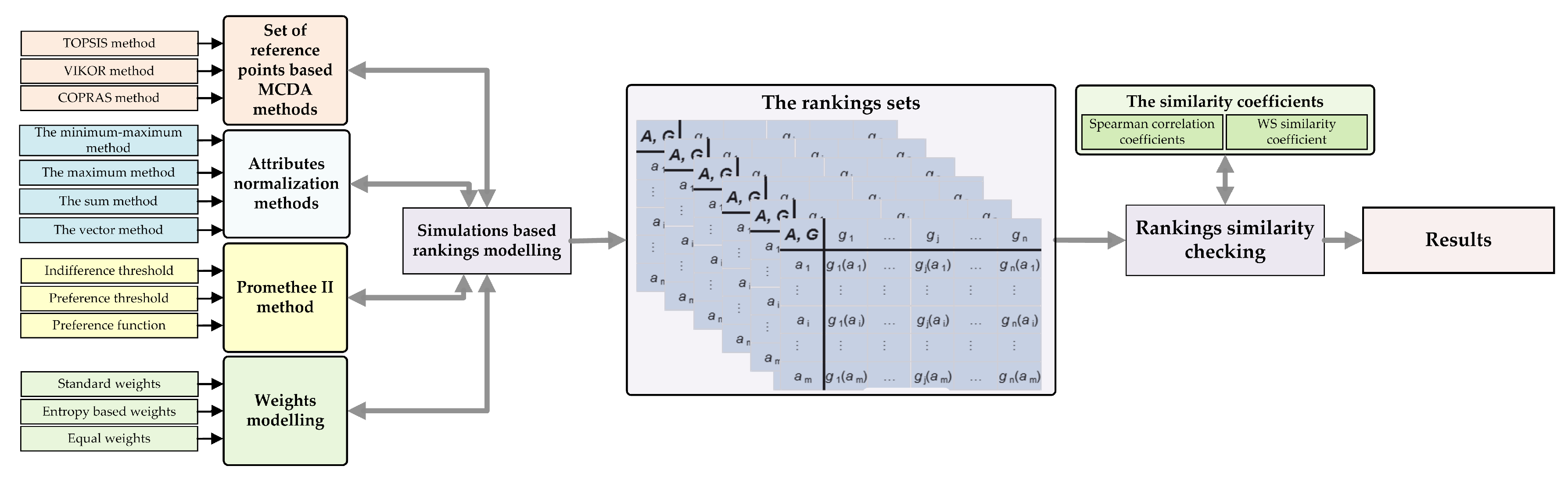
Many methodologies, frameworks, and formal approaches to identify a subset of MCDA methods suitable for the given problem have been developed in prior works [20,22]. The synthesis of available terms is presented later in the article. It should be noted that the assessment of accuracy and reliability of results obtained using various MCDA methods remains a separate research problem. The examples of work on the accuracy assessment and more broadly benchmarking of MCDA methods include Zanakis et al. [24], Chang et al. [29], Hajkowicz and Higgins [30], Żak [31], and others. Their broader discussion is also conducted later in the paper. The authors, focusing their research on selected MCDA methods, effectively use a simulation environment (e.g., Monte Carlo simulation) to generate a set of ranks. The authors most often use Spearman’s rank correlation coefficient to assess and analyze the similarity of the rankings. However, the shortcomings of the indicated approaches should be indicated. In the vast majority of the available literature, the approaches are focused on a given domain of the MCDA method (or a subset of methods) application. Thus, despite the use of a simulation environment, the studies are not comprehensive, limiting the range of obtained results. Most of the papers are focused on the assessment of only selected aspects of the accuracy of single MCDA methods or contain narrow comparative studies of selected MCDA methods. Another important challenge related to multi-criteria decision-making problems that are not included in the works mentioned above is the proper determination of weights [32]. It seems to be an investigation into how various methods to determine criteria weights (subjective weighting methods and objective weighting methods) affect final ranking [33]. In our research, we attempt a complex benchmarking for a subset of carefully selected MCDA methods. Taking care of the correctness and comprehensiveness of the conducted research and at the same time following the guidelines of the authors of publications in this area, we use a simulation environment and apply multiple model input parameters (see Figure 1). The aspects of the conducted analysis and benchmarking of methods include not only the generation of final rankings for a variable number of decision-making options, but also take into account different weighing methods (results obtained using entropy and standard deviation methods) and different techniques of normalizing input data of the MCDA model. The analysis of rank similarities obtained under different conditions and using different MCDA methods was carried out based on reference publications and using Spearman’s ranking correlation coefficient and coefficients.
The study aims to analyze the similarity of rankings obtained using the selected four MCDA methods. It should be noted that in research, we analyze this problem only from the technical (algorithmic) point of view, leaving in the background the conceptual aspects of the method and the systemic assumptions of obtaining model input data. For each of these methods using a simulation environment, several rankings were calculated. The simulation itself was divided into two parts. The first part refers to a comparison of the similarity of the results separately for TOPSIS, VIKOR, COPRAS, and PROMETHEE II. In the second part, these methods were compared with each other. As illustrated in Figure 1), the calculation procedure took into account different normalization methods, weighting methods, preference thresholds, and preference functions. Thus, in the case of the TOPSIS method for each decision matrix, 12 separate rankings were created, where each of them is a different combination of a standardization method and a weighing method. Then, for the same matrix, a set of rankings using other MCDA methods (VIKOR, COPRAS, and PROMETHEE II) was created respectively. This procedure was repeated for different parameters of the decision matrix (in terms of the number of analyzed alternatives and number of criteria). In this way, the simulation provides a complex dataset in which similarities were analyzed using the Spearman and WS coefficients.
In this paper, we used several MCDA methods (TOPSIS, VIKOR, COPRAS, and PROMETHEE II) to make comparative tests. The choice of this set was dictated by the properties and popularity of these methods. These methods and their modifications found an application in many different domains such as sustainability assessment [34,35,36], logistics [37,38,39], supplier selection [7,40,41], manufacturing [42,43,44], environment management [45,46,47], waste management [48,49], energy management [50,51,52,53,54,55], chemical engineering [56,57,58], and many more [59,60]. The choice of a group of TOPSIS, VIKOR, and COPRAS methods is justified, as they form a coherent group of methods of the American MCDA school and are based on the same principles, using the concepts of the so-called reference points. At the same time, unlike other methods of the American school, they are not merely trivial (in the algorithmic sense) elaborations of the simple additional or multiplicative weighted aggregation. The choice of the PROMETHEE II method was dictated by the fact that this method belongs to the European school and that the PROMETHEE II algorithm implements the properties of other European school-based MCDA methods (outranking relations, thresholds, and different preference functions). It should be noted that for benchmarking purposes, the choice of this method has one more justification—unlike other methods of this school, the method provides a full, quantitative final ranking of decision-making options.
The rest of the article is structured as follows. Section 2.1.1 present the most important MCDA foundations. Operational point of view and preference aggregation techniques are presented in Section 2.1.2. Section 2.1.3 and Section 2.1.4 describe respectively American and European-based MCDA methods. Mixed and rule-based methods are shown in Section 2.1.5. Section 2.2 presents the MCDA method selection and benchmarking problem. Section 3.1.1 contains a description of the TOPSIS method and Section 3.1.2 describes the VIKOR method. A description of the COPRAS method can be found in Section 3.1.3 and a description of the PROMETHEE II method is in Section 3.1.4. Section 3.2 describes the normalization methods, which could be applied to data before executing any MCDA methods. Section 3.3 contains a description of weighting methods, which would be used in article. Section 3.4 describes the correlation coefficients that will be used to compare results. The research experiment and the numerical example are presented in Section 4. Section 5 provides the most relevant results and their discussion. Finally, the conclusions are formulated in Section 6.
2. Literature Review
2.1. MCDA State of the Art
In this section, we introduce the methodological assumptions of MCDA, taking into account the operational point of view and available data aggregation techniques. At the same time, we provide an outline of existing methods and decision-making schools.
2.1.1. MCDA Foundations
Almost in every case, the nature of the decision problem makes it a multi-criteria problem. This means that making a “good” decision requires considering many decision options, where each option should be considered in terms of many factors (criteria) that characterize its acceptability. The values of these factors may limit the number of variants in case their values exceed the assumed framework. They can also serve for grading the admissibility of variants in the situation when each of them is admissible, and the multi-criteria problem consists in choosing subjectively the best of them. For different decision makers, different criteria may have a different relevance, so in no case can a multi-criteria decision be considered as completely objective. Only the ranking of individual variants with given weights of individual criteria is objective here, as this ranking is usually generated using a specific multi-criteria method. Therefore, concerning recommended multi-criteria decisions, the term “optimal” is not used but ”most satisfactory decision-maker” [23] which means optimum in the sense of Pareto [2]. In conclusion, it can be concluded that multi-criteria models should take into account elements that can be described as a multi-criteria paradigm: The existence of multiple criteria, the existence of conflicts between criteria, and the complex, subjective, and poorly structured nature of the decision-making problem [61].
The MCDA methods are used to solve decision problems where there are many criteria. The literature provides various models of the decision-making process, e.g., Roy, Guitouni, and Keeney. For example, Guitouni’s model distinguishes five stages: Decision problem structuring, articulating and modeling preferences, preference aggregation, exploitation of aggregation, and obtaining a solution recommendation [62]. The essential elements of a multi-criteria decision problem are formed by a triangle (A, C, and E), where A defines a set of alternative decision options, C is a set of criteria, while E represents the criteria performance of the options [62]. Modeling of the decision maker’s preferences can be done in two ways, i.e., directly or indirectly, using the so-called disaggregation procedures [63]. The decision maker’s preferences are expressed using binary relations. When comparing decision options, two fundamental indifference relations ( I ) and strict preference ( P ) may occur. Moreover, the set of basic preferential relations may be extended by the relations of a weak preference of one of the variants to another and their incomparability (variants) [64], creating together with the basic relations the so-called outranking relation.
2.1.2. Operational Point of View and Preference Aggregation Techniques
The structured decision problem, for which the modeling of the decision maker’s preferences was carried out, is an input for the multi-criteria preference aggregation procedure (MCDA methods). This procedure should take into account the preferences of the decision-maker, modeled using the weighting of criteria, and preference thresholds. This procedure is responsible for aggregating the performance of the criteria of individual variants to obtain a global result of comparing the variants consistent with one of the multi-criteria issues. The individual aggregation procedures can be divided according to their operational approach. In the literature three main approaches exist [63]:
- The use of a single synthesized criterion: In this approach, the result of the variants’ comparisons is determined for each criterion separately. Then the results are synthesized into a global assessment. The full order of variants is obtained here [65];
- The synthesis of the criteria based on the relation of outranking: Due to the occurrence of incomparability relations, this approach allows for obtaining the partial order of variants [65];
The difference between the use of a single synthesized criterion and the synthesis based on the relation of exceedance is that in methods using synthesis to one criterion there is a compensation, while methods using the relation of exceedance by many researchers are considered uncompensated [68,69].
Research on multi-criteria decision support has developed two main groups of methods. These groups can be distinguished due to the operational approach used in them. These are the methods of the so-called American school of decision support and the methods of the European school [70,71]. There is also a group of so-called basic methods, most of which are similar in terms of the operational approach to the American school methods. Examples of basic methods are the lexicographic method, the ejection method for the minimum attribute value, the maximum method, or the additive weighting method. Besides, there is a group of methods combining elements of the American and European approaches, as well as methods based on the previously mentioned rule approach.
2.1.3. American School-Based MCDA Methods
The methods of the American school of decision support are based on a functional approach [63], namely, the use of value or usability. These methods usually do not take into account the uncertainty, inaccuracy, and uncertainty that can occur in data or decision-maker preferences [1]. This group of methods is strongly connected with the operational approach using a single synthesized criterion. The basic methods of the American school are MAUT, AHP, ANP, SMART, UTA, MACBETH (Measuring Attractiveness by a Categorical Based Evaluation Technique), or TOPSIS.
In the MAUT method, the most critical assumption is that the preferences of the decision-maker can be expressed using a global usability function, taking into account all the criteria taken into account. The AHP method is the best known and most commonly used functional method. This method allows one to prioritize the decision-making problem. The ANP method is a generalization of AHP. Instead of prioritizing the decision problem, it allows the building of a network model in which there may be links between criteria and variants and their feedback. In the SMART method, the criteria values of variants are converted to a common internal scale. This is done mathematically by the decision-maker, and the value function is used [72]. In the UTA method, the decision maker’s preferences are extracted from the reference set of variants [73]. The MACBETH method (Measuring Attractiveness by a Categorical Based Evaluation Technique) is based on qualitative evaluations. The individual variants are compared here in a comparison matrix in pairs. The criterion preferences of the variants are aggregated as a weighted average [74,75]. In the TOPSIS (Technique for Order Preference by Similarity to Ideal Solution) method, the decision options considered are compared for the ideal and the anti-ideal solution [76,77,78,79].
2.1.4. European School-Based MCDA Methods
The methods of the European School use a relational model. Thus, they use a synthesis of criteria based on the relation of outranking. This relation is characterized by transgression between pairs of decision options. Among the methods of the European School of Decision Support, the groups of ELECTRE and PROMETHEE methods should be mentioned above all [1].
ELECTRE I and ELECTRE Is methods are used to solve the selection problem. In the ELECTRE I method there is a true criterion (there are no indifference and preference thresholds), while in ELECTRE Is, pseudo-criteria have been introduced including thresholds. It should be noted here that indifference and preference thresholds can be expressed directly as fixed quantities for a given criterion or as functions, which would allow distinguishing the relation of weak and strong preferences. The relations of the excess occurring between the variants are presented on the graph and the best variants are those which are not exceeded by any other [80,81]. The ELECTRE II method is similar to the ELECTRE I since no indifference and preference thresholds are defined here as well, i.e., the true criteria are also present here. Furthermore, the calculation algorithm is the same almost throughout the procedure. However, the ELECTRE II method distinguishes weak and strong preference [82]. The ELECTRE III method is one of the most frequently used methods of multi-criteria decision support and it deals with the ranking problem. The ELECTRE IV method is similar to ELECTRE III in terms of using pseudo-criteria. Similarly, the final ranking of variants is also determined here. The ELECTRE IV method determines two orders (ascending and descending) from which the final ranking of variants is generated. However, the ELECTRE IV method does not define the weights of criteria, so all criteria are equal [83]. ELECTRE Tri is the last of the discussed ELECTRE family methods. It deals with the classification problem and uses pseudo-criteria. This method is very similar to ELECTRE III in procedural terms. However, in the ELECTRE Tri method, the decisional variants are compared with so-called variants’ profiles, i.e., “artificial variants” limiting particular quality classes [84].
PROMETHEE methods are used to determine a synthetic ranking of alternatives. Depending on the implementation, they operate on true or pseudo-criteria. The methods of this family combine most of the ELECTRE methods as they allow one to apply one of the six preference functions, reflecting, among others, the true criterion and pseudo-criteria. Moreover, they enrich the ELECTRE methodology at the stage of object ranking. These methods determine the input and output preference flows, based on which we can create a partial ranking in the PROMETHEE I method [85]. In contrast, in the PROMETHEE II method, the net preference flow values for individual variants are calculated based on input and output preference flows. Based on net values, a complete ranking of variants is determined [86,87].
NAIADE (Novel Approach to Imprecise Assessment and Decision Environment) methods are similar to PROMETHEE in terms of calculation because the ranking of variants is determined based on input and output preference flows [88]. However, when comparing the variants, six preferential relations defined based on trapezoidal fuzzy numbers are used (apart from indistinguishability of variants, weak, and strong preference is distinguished). The methods of this family do not define the weights of criteria [89].
Other examples of methods from the European MCDA field are ORESTE, REGIME, ARGUS, TACTIC, MELCHIOR, or PAMSSEM. The ORESTE method requires the presentation of variant evaluations and a ranking of criteria on an ordinal scale [90]. Then, using the distance function, the total order of variants is determined concerning the subsequent criteria [91]. The REGIME method is based on the analysis of variants’ compatibility. The probability of dominance for each pair of variants being compared is determined and on this basis the order of variants is determined [92]. In the ARGUS method for the representation of preferences on the order scale, qualitative measures are used [93]. The TACTIC method (Treatment of the Alternatives According To the Importance of Criteria) is based on quantitative assessments of alternatives and weights of criteria. Furthermore, it allows the use of true criteria and quasi-criteria, thus using the indistinguishability threshold as well as the veto. Similarly to ELECTRE I, TACTIC and ARGUS methods use preference aggregation based on compliance and non-compliance analysis [94]. In the MELCHIOR method pseudo-criteria are used, the calculation is similar to ELECTRE IV, while in the MELCHIOR method the order relationship between the criteria is established [93]. The PAMSSEM I and II methods are a combination of ELECTRE III, NAIADE, and Promethee and implement the computational procedure used in these methods [95,96].
2.1.5. Mixed and Rule-Based Methods
Many multi-criteria methods combine the approaches of the American and European decision support school. An example is the EVAMIX method [23], which allows taking into account both quantitative and qualitative criteria, using two separate measures of domination [97]. Another mishandled method is the QUALIFLEX method [98], which allows for the use of qualitative evaluations of variants and both quantitative and qualitative criteria weights [99]. PCCA (Pairwise Criterion Comparison Approach) methods can be treated as a separate group of multi-criteria methods. They focus on the comparison of variants concerning different pairs of criteria considered instead of single criteria. The partial results obtained in this way are then aggregated into the evaluation and final ranking [100]. The methods are based on the PCCA approach: MAPPAC, PRAGMA, PACMAN, and IDRA [101].
The last group of methods are methods based strictly on decision rules [102]. These are methods using fuzzy sets theory (COMET: Characteristic Objects Method) [22] and rough sets theory (DRSA: (Dominance-based Rough Set Approach) [103]. In the methods belonging to this group, the decision rules are initially built. Then, based on these rules, variants are compared and evaluated, and a ranking is generated.
The COMET (Characteristic Objects Method) requires giving fuzzy triangular numbers for each criterion [104], determining the degree of belonging of variants to particular linguistic values describing the criteria [105]. Then, from the values of vertices of particular fuzzy numbers, the characteristic variants are generated. These variants are compared in pairs by the decision-maker, and their model ranking is generated. These variants, together with their aggregated ranking values, create a fuzzy rule database [21]. After the decision system of the considered variants is given to the decision system, each of the considered variants activates appropriate rules and its aggregated rating is determined as the sum of the products of the degrees in which the variants activate individual rules [106,107].
The DRSA method (Dominance-based Rough Set Approach) is based on the rough set theory and requires the definition of a decision table taking into account the values of criteria and consequences of previous decisions (in other words, the table contains historical decision options together with their criteria assessments as well as their aggregated global assessments) [108]. The decision defines the relation of exceedance. The final assessment of a variant is determined as the number of variants which, based on the rules, the considered variant exceeds or is not exceeded by. Moreover, the number of variants that are exceeded or not exceeded by the considered variant is deducted from the assessment [109,110].
2.2. MCDA Methods Selection and Benchmarking Problem
The complexity of the problem of choosing the right multi-criteria method to solve a specific decision problem results in numerous works in the literature where this issue is addressed. These works can be divided according to their approach to method selection. Their authors apply approaches based on benchmarks, multi-criteria analysis, and informal and formal structuring of the problem or decision-making situation. An attempt at a short synthesis of available approaches to the selection of MCDA methods to a decision-making problem is presented below.
The selection of a method based on multi-criteria analysis requires defining criteria against which individual methods will be evaluated. This makes it necessary to determine the structure of the decision problem at least partially [111]. Moreover, it should be noted that treating the MCDA method selection based on the multi-criteria approach causes a looping of the problem, because for this selection problem, the appropriate multi-criteria method should also be chosen [112]. Nevertheless, the multi-criteria approach to MCDA method selection is used in the literature. Examples include works by Gershon [113], Al-Shemmeri et al. [111], and Celik and Deha Er [114].
The informal approach to method selection consists of selecting the method for a given decision problem based on heuristic analysis performed by the analyst/decision-maker [115]. This analysis is usually based on the author’s thoughts and unstructured description of the decision problem and the characteristics of particular methods. The methodological approach is similar to the semi-formal one, with the difference that the characteristics of individual MCDA methods are to some extent formalized here (e.g., table describing the methods). The informal approach was used in Adil et al. [115] and Bagheri Moghaddam et al. [116]. The semi-formal approach has been used in the works of Salinesi and Kornyshov [117], De Montis et al. [118], and Cinelli et al. [119].
In the formal approach to the selection of the MCDA method, the description of individual methods is fully structured (e.g., taxonomy or a table of features of individual MCDA methods) [120,121]. The decision problem and the method of selecting a single or group of MCDA methods from among those considered are formally defined (e.g., based on decision rules [122], artificial neural networks [123], or decision trees [23,124]). These are frameworks, which enable a selection of MCDA method based on the formal description of methods and decision problem. Such an approach is proposed, among others, in works: Hwang and Yoon [125], Moffett and Sarkar [124], Guitouni and Martel [23], Guitouni et al. [62], Wątróbski [120], Wątróbski and Jankowski [122], Celik and Topcu [126], Cicek et al. [127], and Ulengin et al. [123].
The benchmarking approach seems particularly important. It focuses on a comparison of the results obtained by individual methods. The main problem of applying this approach is to find a reference point against which the results of the examined multi-criteria methods would be compared. Some authors take the expert ranking as a point of reference whilst others compare the results to the performance of one selected method or examine the compliance of individual rankings obtained using particular MCDA methods. Examples of benchmark-based approach to selection/comparison of MCDA methods are works: Zanakisa et al. [24], Chang et al. [29] Hajkowicz and Higgins [30], and Żak [31].
The publication of Zanakis et al. [29] presents results of benchmarks for eight MCDA methods (Simple Additive Weighting, Multiplicative Exponential Weighting, TOPSIS, ELECTRE, and four AHP variants). In the simulation test scenario, randomly generated decision problems were assumed in which the number of variants was equal: 3, 5, 7, and 9; the number of criteria were: 5, 10, 15, and 20; and the weights of the criteria could be equal, have a uniform distribution in the range <0; 1> with a standard deviation of 1/12, or a beta U-shaped distribution in the range <0; 1> with a standard deviation of 1/24. Moreover, the assessments of alternatives were randomly generated according to a uniform distribution in the range <0; 1>. The number of repetitions was 100 for each combination of criteria, variants, and weights. Therefore, 4800 decision problems were considered in the benchmark (4 number of criteria × 4 number of variants × 3 weightings types × 100 repetitions) and 38,400 solutions were obtained in total (4800 problems × 8 MCDA methods). Within the tests, the average results of all rankings generated by each method were compared with the average results of rankings generated by the SAW method, which was the reference point. Comparisons were made using, among others, Spearman’s rank correlation coefficient for rankings.
Benchmark also examined the phenomenon of ranking reversal after introducing an additional non-dominant variant to the evaluation. The research on the problem of ranking reversal was carried out based on similar measures, with the basic ranking generated by a given MCDA method being the point of reference in this case. The authors of the study stated that the AHP method gives the rankings closest to the SAW method, while in terms of ranking reversal, the TOPSIS method turned out to be the best.
Chang et al. [29] took up a slightly different problem. They presented the procedure of selecting a group fuzzy multi-criteria method generating the most preferred group ranking for a given problem. The authors defined 18 fuzzy methods, which are combinations of two methods of group rating averaging (arithmetic and geometric mean), three multi-criteria methods (Simple Additive Weighting, Weighted Product, and TOPSIS), and three methods of results defuzzification (Center-of-area, graded mean integration, and metric distance). The best group ranking was selected by comparing each of the 18 rankings with nine individual rankings of each decision maker created using methods that are a combination of multi-criteria procedures and defuzzification methods. Spearman’s correlation was used to compare group and individual rankings.
In the work of Hajkowicz and Higgins [30] rankings were compared using five methods (Simple Additive Weighting, Range of Value Method, PROMETHEE II, Evamix, and Compromise programming). To compare the rankings, we used Spearman’s and Kendall’s correlations for full rankings and a coefficient that directly determines the compliance on the first three positions of each of the compared rankings. The study considered six decision-making problems, in the field of water resources management, undertaken in the scientific literature. Nevertheless, it should be noted that this statement is based on the analysis of features and possibilities offered by individual MCDA methods. However, it does not result from the conducted benchmark.
Another publication cited in which the benchmark was applied to the work of Żak [31]. The author considered five multi-criteria methods (ELECTRE, AHP, UTA, MAPPAC, and ORESTE). The study was based on the examination of the indicated methods concerning three decision-making problems related to transport, i.e., (I) evaluation of the public transportation system development scenarios, (II) ranking of maintenance and repair contractors in the public transportation system, and (III) selection of the means of transport used in the public transportation system. The benchmark uses expert evaluations for each of the methods in terms of versatility and relevance to the problem, computational performance, modeling capabilities for decision-makers, reliability, and usefulness of the ranking.
The problem of MCDA methods benchmarking is also addressed in many up-to-date studies. Thus in the paper [128] using building performance simulation reliability of rankings generated using AHP, TOPSIS, ELECTRE III, and PROMETHEE II methods was evaluated. In the paper [129] using Monte Carlo simulation, Weighted Sum, and Weighted Product Methods (WSM/WPM), TOPSIS, AHP, PROMETHEE I, and ELECTRE I were compared. The next study [130] adopted the same benchmarking environment as in the study [24]. The authors empirically compare the rankings produced by multi-MOORA, TOPSIS, and VIKOR methods. In the paper [131] another benchmark of selected MCDA methods was presented. AHP, Fuzzy AHP, TOPSIS, Fuzzy TOPSIS, and PROMETHEE I methods were used here. The similarity of rankings was evaluated using Spearman’s rank correlation coefficient. In the next paper [132], the impact of different uncertainty sources on the rankings of MCDA problems in the context of food safety was analyzed. In this study, MMOORA, TOPSIS, VIKOR, WASPAS, and ELECTRE II were compared. In the last example work [133], using a simulation environment, the impact of different standardization techniques in the TOPSIS method on the final form of final rankings was examined. The above literature analysis unambiguously shows the effectiveness of the simulation environment in benchmarking methods from the MCDA family. However, at the same time, it constitutes a justification for the authors of this article for the research methods used.
3. Preliminaries
3.1. MCDA Methods
In this section, we introduced formal foundations of MCDA methods used during the simulation. We selected three methods belonging to the American school (TOPSIS, VIKOR, and COPRAS) and one popular method of the European school called PROMETHEE II.
3.1.1. TOPSIS
The first one is Technique of Order Preference Similarity (TOPSIS). In this approach, we measure the distance of alternatives from the reference elements, which are respectively positive and negative ideal solution. This method was widely presented in [9,134]. The TOPSIS method is a simple MCDA technique used in many practical problems. Thanks to its simplicity of use, it is widely used in solving multi-criteria problems. Below we present its algorithm [9]. We assume that we have a decision matrix with m alternatives and n criteria is represented as .
Step 1. Calculate the normalized decision matrix. The normalized values calculated according to Equation (1) for profit criteria and (2) for cost criteria. We use this normalization method, because [11] shows that it performs better than classical vector normalization. Although, we can also use any other normalization method.
Step 2. Calculate the weighted normalized decision matrix according to Equation (3).
Step 3. Calculate Positive Ideal Solution (PIS) and Negative Ideal Solution (NIS) vectors. PIS is defined as maximum values for each criteria (4) and NIS as minimum values (5). We do not need to split criteria into profit and cost here, because in step 1 we use normalization which turns cost criteria into profit criteria.
Step 4. Calculate distance from PIS and NIS for each alternative. As shown in Equations (6) and (7).
Step 5. Calculate each alternative’s score according to Equation (8). This value is always between 0 and 1, and the alternatives which have values closer to 1 are better.
3.1.2. VIKOR
VIKOR is an acronym in Serbian that stands for VlseKriterijumska Optimizacija I Kompromisno Resenje. The decision maker chooses an alternative that is the closest to the ideal and the solutions are assessed according to all considered criteria. The VIKOR method was originally introduced by Opricovic [135] and the whole algorithm is presented in [134]. These both methods are based on closeness to the ideal objects [136]. However, they differ in their operational approach and how these methods consider the concept of proximity to the ideal solutions.
The VIKOR method, similarly to the TOPSIS method, is based on distance measurements. In this approach a compromise solution is sought. The description of the method will be quoted according to [135,136]. Let us say that we have a decision matrix with m alternatives and n criteria is represented as . Before actually applying this method, the decision matrix can be normalized with one of the methods described in Section 3.2.
Step 1. Determine the best and the worth values for each criteria functions. Use (9) for profit criteria and (10) for cost criteria.
Step 3. Compute the values using Equation (13).
where
and v is introduced as a weigh for the strategy “majority of criteria”. We use here.
Step 4. Rank alternatives, sorting by the values S, R, and Q in ascending order. Result is three ranking lists.
3.1.3. COPRAS
Third used method is a COPRAS (Complex Proportional Assessment), introduced by Zavadskas [137,138]. This approach assumes a direct and proportional relationship of the importance of investigated variants on a system of criteria adequately describing the decision variants and on values and weights of the criteria [139]. This method ranks alternatives based on their relative importance (weight). Final ranking is creating using the positive and negative ideal solutions [138,140]. Assuming, that we have a decision matrix with m alternatives and n criteria is represented as , the COPRAS method is defined in five steps:
Step 1. Calculate the normalized decision matrix using Equation (14).
Step 2. Calculate the difficult normalized decision matrix, which represents a multiplication of the normalized decision matrix elements with the appropriate weight coefficients using Equation (15).
Step 3. Determine the sums of difficult normalized values, which was calculated previously. Equation (16) should be used for profit criteria and Equation (17) for cost criteria.
where k is the number of attributes that must be maximized. The rest of attributes from to n prefer lower values. The and values show the level of the goal achievement for alternatives. A higher value of means that this alternative is better and the lower value of also points to better alternative.
Step 4. Calculate the relative significance of alternatives using Equation (18).
Step 5. Final ranking is performed according values (19).
where stands for the maximum value of the utility function. Better alternatives have a higher value, e.g., the best alternative would have .
3.1.4. PROMETHEE II
The Preference Ranking Organization Method for Enrichment of Evaluations (PROMETHEE) is a family of MCDA methods developed by Brans [18,141]. It is similar to other methods input data, but it optionally requires to choose preference function and some other variables. In this article we use PROMETHEE II method, because the output of this method has a full ranking of the alternatives. It is the approach where a complete ranking of the actions is based on the multi-criteria net flow. It includes preferences and indifferences (preorder) [142]. According to [134,141], PROMETHEE II is designed to solve the following multicriteria problems:
where A is a finite set of alternatives and is a set of evaluation criteria either to be maximized or minimized. In other words, is a value of criteria i for alternative . With these values and weights we can define evaluation table (see Table 1).
Step 1. After defining the problem as described above, calculate the preference function values. It is defined as (21) for profit criteria.
where is the difference between two actions (pairwise comparison):
and the value of the preference function P is always between 0 and 1 and it is calculating for each criterion. The Table 2 presents possible preference functions.
This preference functions and variables such as p and q allows one to customize the PROMETHEE model. For our experiment these variables are calculated according to Equations (23) and (24):
where D is a positive value of the d values (22) for each criterion and k is a modifier. In our experiments .
Step 2. Calculate the aggregated preference indices (25).
where a and b are alternatives and shows how much alternative a is preferred to b over all of the criteria. There are some properties (26) which must be true for all alternatives set A.
Step 4. In this article we will use only PROMETHEE II, which results in a complete ranking of alternatives. Ranking is based on the net flow (29).
Larger value of means better alternative.
3.2. Normalization Methods
In the literature, there is no clear assignment to which decision-makers’ methods of data normalization are used. This situation poses a problem, as it is necessary to consider the influence of a particular normalization on the result. The most common normalization methods in MCDA methods can be divided into two groups [143], i.e., methods designed to profit (30), (32), (34) and (36) and cost criteria (31), (33), (35), and (37).
The minimum-maximum method: In this approach, the greatest and the least values in the considered set are used. The formulas are described as follows (30) and (31):
The maximum method: In this technique, only the greatest value in the considered set is used. The formulas are described as follows (32) and (33):
3.3. Weighting Methods
In this section, we present three popular methods related to objective criteria weighting. These are the most popular methods currently found in the literature. In the future, this set should be extended to other methods.
3.3.1. Equal Weights
The first and least effective weighted method is the equal weight method. All criteria’s weights are equal and calculated by Equation (38), where n is the number of criteria.
3.3.2. Entropy Method
3.3.3. Standard Deviation Method
3.4. Correlation Coefficients
Correlation coefficients make it possible to compare obtained results and determine how similar they are. In this paper we compare ranking lists obtained by several MCDA methods using Spearman rank correlation coefficient (44), weighted Spearman correlation coefficient (46), and rank similarity coefficient (47).
3.4.1. Spearman’s Rank Correlation Coefficient
3.4.2. Weighted Spearman’s Rank Correlation Coefficient
For a sample of size N, rank values and are defined as (46). In this approach, the positions at the top of both rankings are more important. The weight of significance is calculated for each comparison. It is the element that determines the main difference to the Spearman’s rank correlation coefficient, which examines whether the differences appeared and not where they appeared.
3.4.3. Rank Similarity Coefficient
4. Study Case and Numerical Examples
The main goal of the experiments is to test if the MCDA method or weight calculation method has an impact on the final ranking and how significant this impact is. For this purpose, we applied four commonly used classical MCDA methods, which are listed in Section 3.1. In the case of TOPSIS and VIKOR methods, we would use different normalization methods, and for the PROMETHEE method, we use various preference function and use different p and q values. The primary way to analyze the results obtained from numerical experiments is to use selected correlation coefficients, described in Section 3.4.
Algorithm 1 presents the simplified pseudo-code of the experiment, where we process matrices with different number of criteria and alternatives. The number of criteria changed from 2 to 5 and the number of the alternatives belongs to the set . For each of the 20 combinations, the number of alternatives and criteria was generated after 1000 random decision matrices. They contain attribute values for all analyzed alternatives for all analyzed criteria. The preference values of the drawn alternatives are not known, but three different vectors of criteria weights are derived from this data. Rankings are then calculated using these different methods with different settings. This way, we obtain research material in the form of rankings calculated using different approaches. Analyzing the results using similarity coefficients, we try to determine the similarity of the obtained results. For each matrix we perform the following steps:
- Step 1.
- Calculate 3 vectors of weights, using equations described in Section 3.3;
- Step 2.
- Split criteria into profit and cost criteria: Assuming we have n criteria, first are considered to be profit criteria and the rest ones are considered to be cost;
- Step 3.
- Compute 3 rankings using MCDA methods listed in Section 3.1 and three different weighting vectors.
| Algorithm 1 Research algorithm |
|
The further part of this section presents two examples that are intended to explain our simulation study better. The sample data and how it is handled in the following section will be reviewed. Due to the vast number of generated results, some figures have been placed in the Appendix A for clarity.
4.1. Decision Matrices
We have chosen two random matrices with three criteria and five alternatives to show how exactly these matrices are processed during the experiment. These matrices were chosen to demonstrate how many different or similar the rankings obtained with different MCDA methods in particular cases could be. Table 3 and Table A1 contain chosen matrices and their weights which was calculated with three different methods described in Section 3.3. In the following sections, the example from Table 3 will be discussed separately for clarity. The results for the second example (Table A1) will be shown in the Appendix B.
4.2. TOPSIS
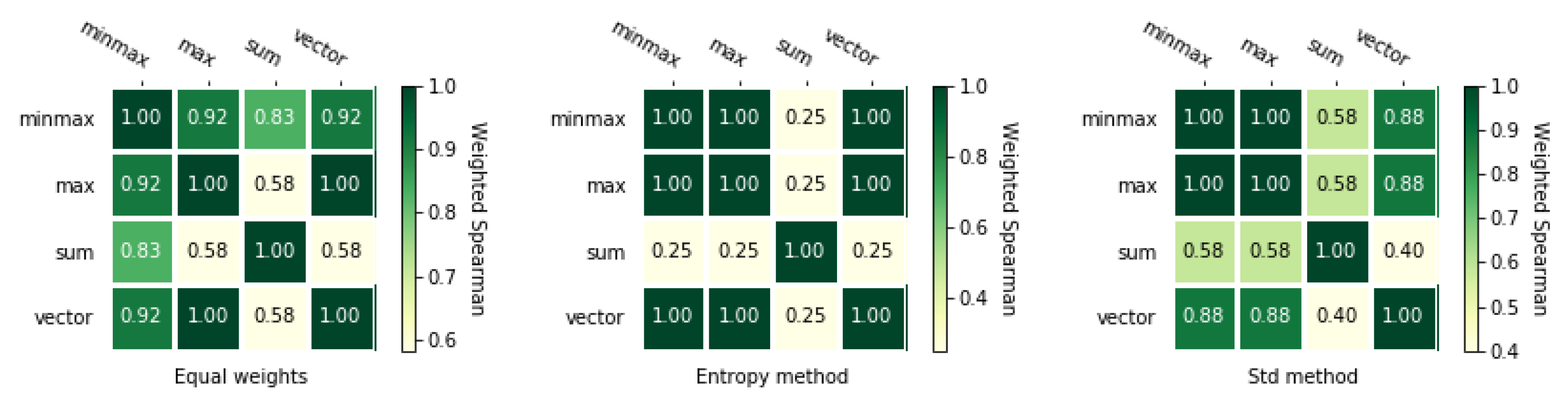
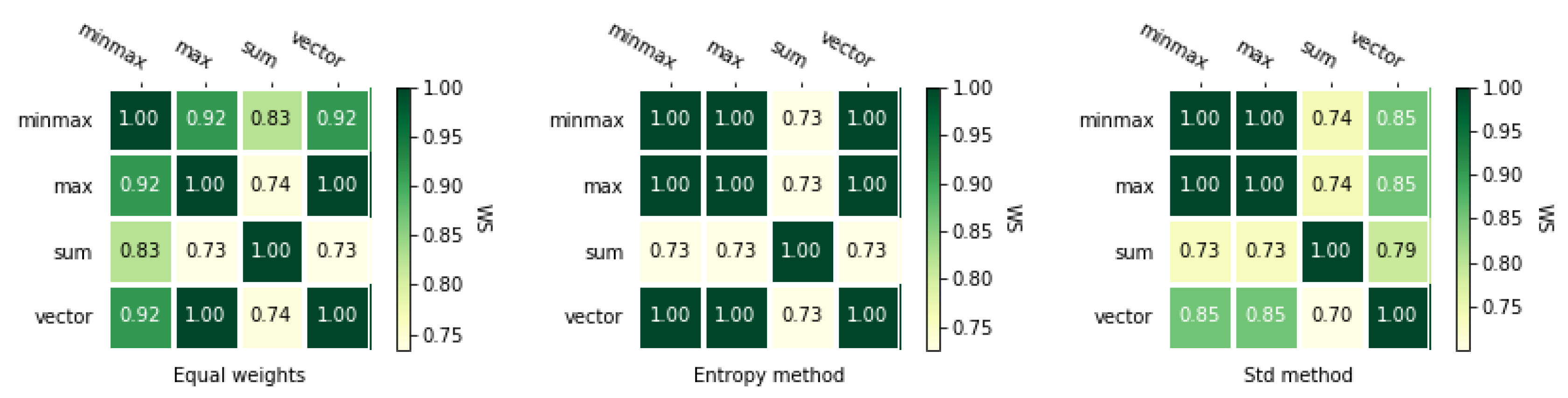
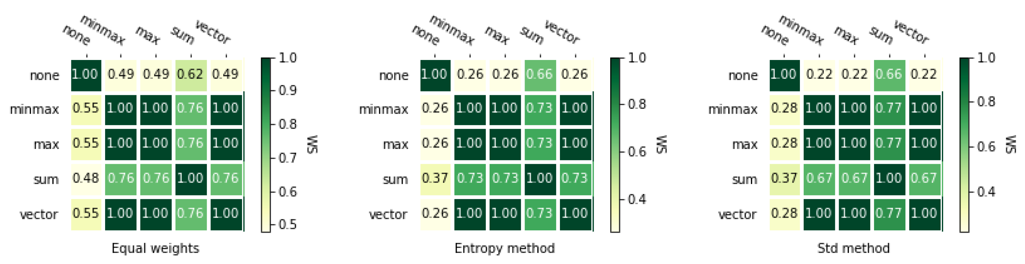
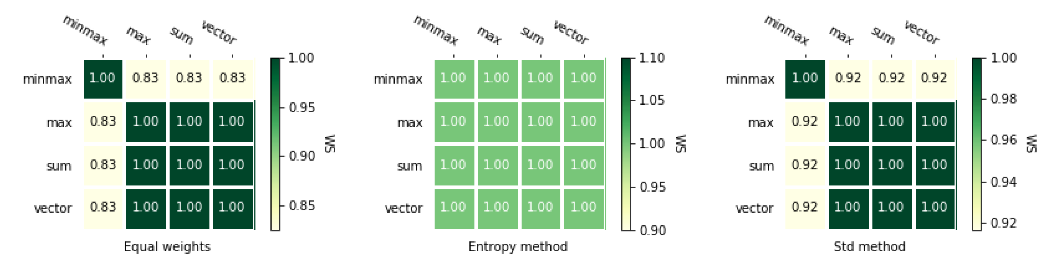
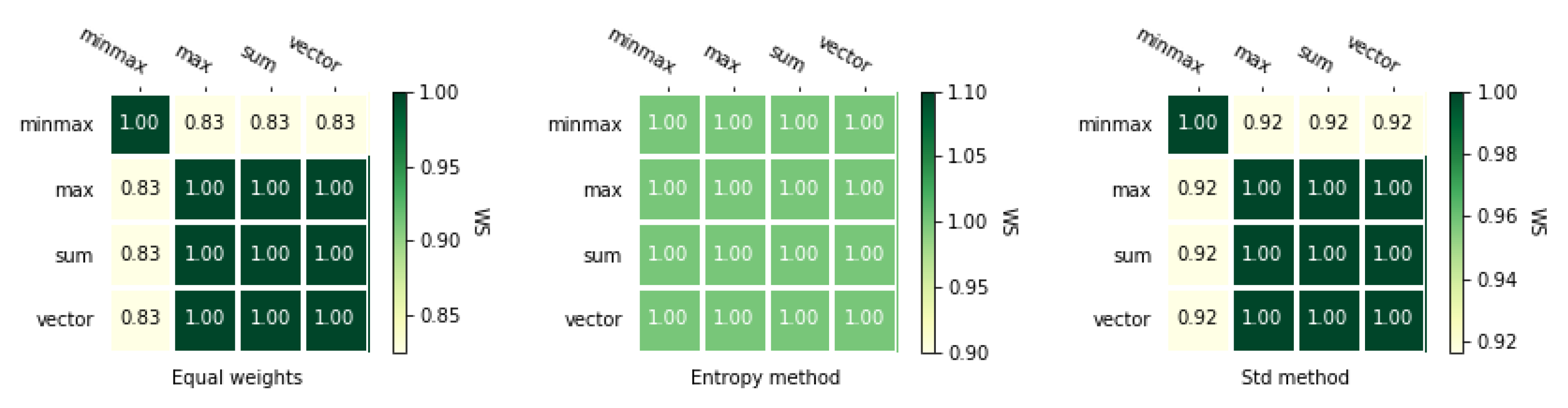
Processing a matrix with the TOPSIS method, using four different normalization methods and three different weighting methods gives us 12 rankings. Table 4 presents all rankings for the analyzed example showed in Table 4, and rankings for the second example are shown in Table A2. The orders in both cases are not identical and we can observe that the impact of different parameters varies for almost every case in the first example (Table 3). It depends mainly on the applied normalization method and selected weight vector. However, we need to determine exactly the similarity of considered rankings. Therefore, we use coefficients similarity, which are presented in heat maps in Figure 2 and Figure 3. The results for the second numerical example is presented in Figure A1 and Figure A2. These figures show exactly how different these rankings are using the and coefficients described in Section 3.4. Each figure shows three heat maps corresponding to three weighting methods.
Figure 2 and Figure 3 presents and correlations between rankings obtained using different normalization methods with TOPSIS method. The most significant difference is obtained for the ranking calculated using the entropy method and sum-based normalization. Only a single discrepancy appears for the alternatives and while comparing this ranking with the rest of the rankings. There is a change in the ranking on positions 2 and 5. These figures also show that the coefficient is asymmetrical as opposed to . Therefore both coefficients will also be used in further analyses.
Next, Figure A1 and Figure A2 show and correlations for the second matrix. Rankings obtained using different normalization methods with TOPSIS are far more correlated than for the first matrix. The entropy methods weights gave as equal rankings and the ranking for the minmax normalization method is slightly different for equal weights and standard deviation weighting method.
4.3. VIKOR
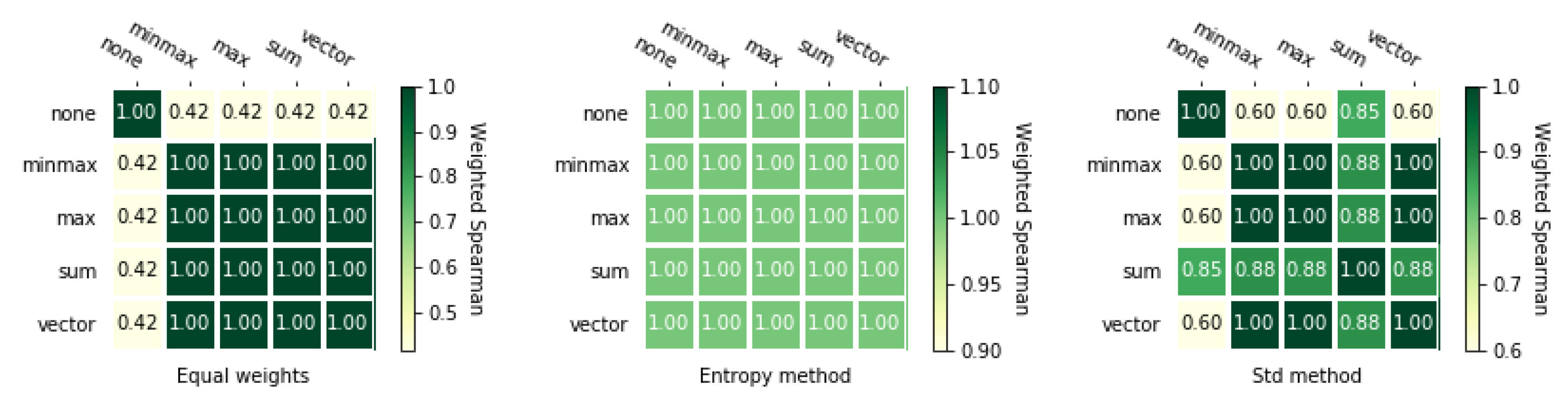
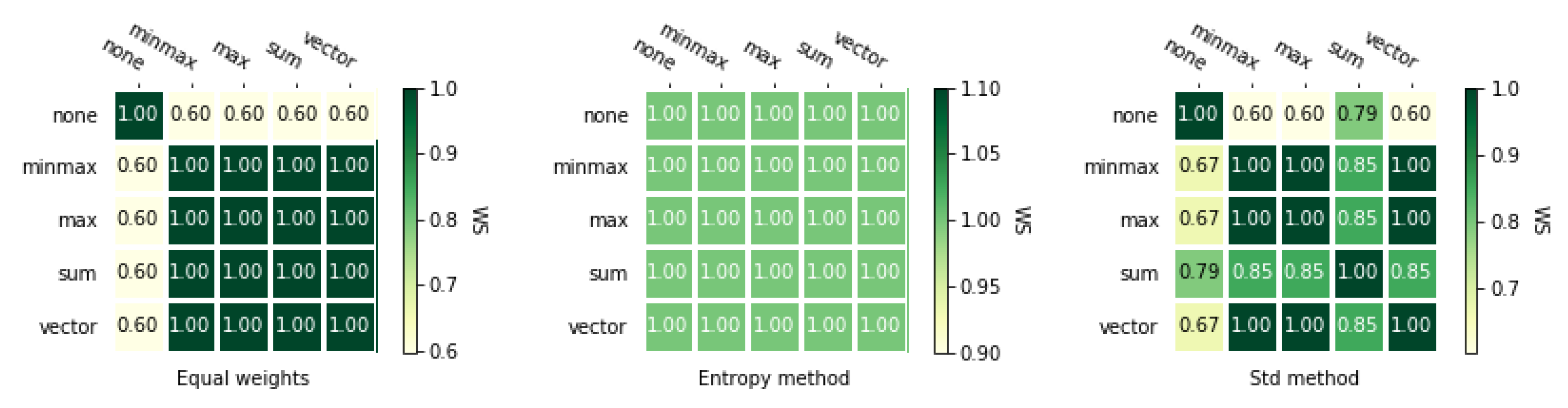
Next, we calculate rankings for both matrices using the VIKOR method in combination with four different normalization methods and three weighting methods. Besides, we also use VIKOR without normalization (represented by “none” in the tables and on the figures). Rankings are shown in Table 5 and Table A3. These rankings have more differences between themselves than the rankings obtained using TOPSIS method with different normalization methods.
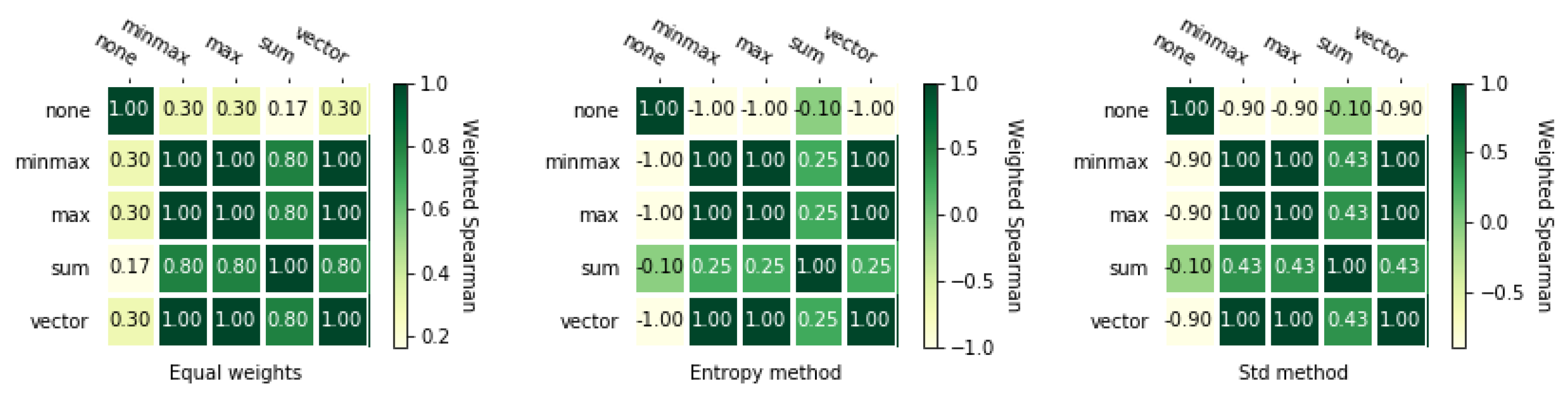
Figure 4 and Figure 5 with and correlation coefficients show us that in this case the entropy weighting method performed worse than the other two weighting methods. In addition, it is noticeable how small size of the correlation between VIKOR without normalization. For the entropy weighting method, the value is which means that rankings obtained with VIKOR without normalization are reversed to VIKOR with any other normalization methods.
The rankings calculated for the second matrix are more correlated between themselves, which is presented on heat maps Figure A2 and Figure A3. Similarly to TOPSIS, the entropy weighted method gives perfectly correlated rankings and the other two weighting method gives us fewer correlated rankings. Moreover, it is noticeable that the ranking obtained using VIKOR without normalization is less correlated to VIKOR with normalization methods.
4.4. PROMETHEE II
For exemplary purposes, we use the PROMETHEE II method with five different preference functions, and the q and p values for them are calculated as follows:
where D stands for positive values of the differences (see Section 3.1.4 for a more detailed explanation). As previously mentioned, Table 6 and Table A4 contains rankings obtained using different preference functions and different weighting methods.
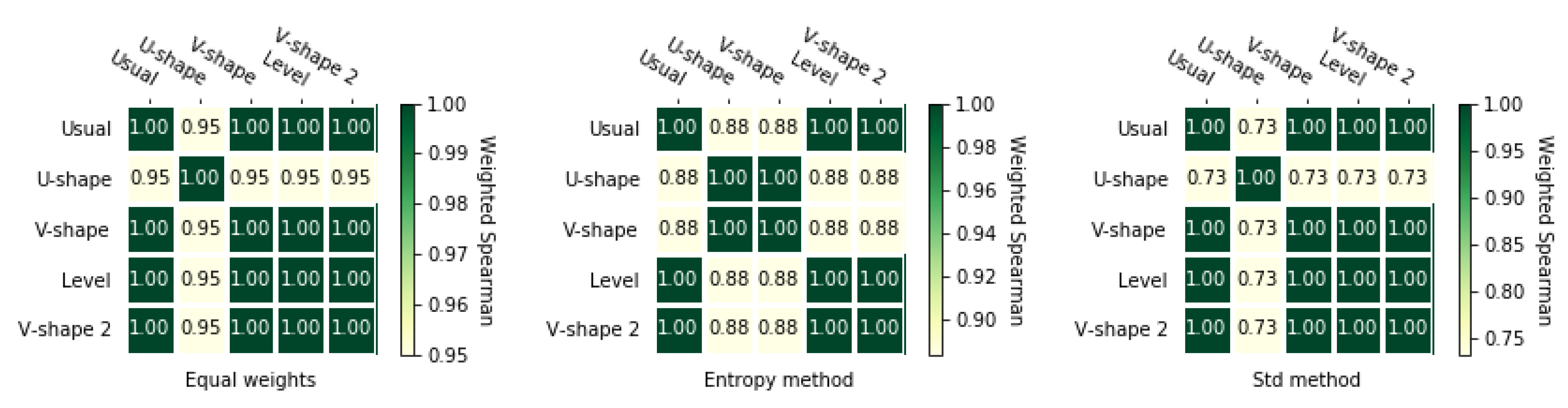
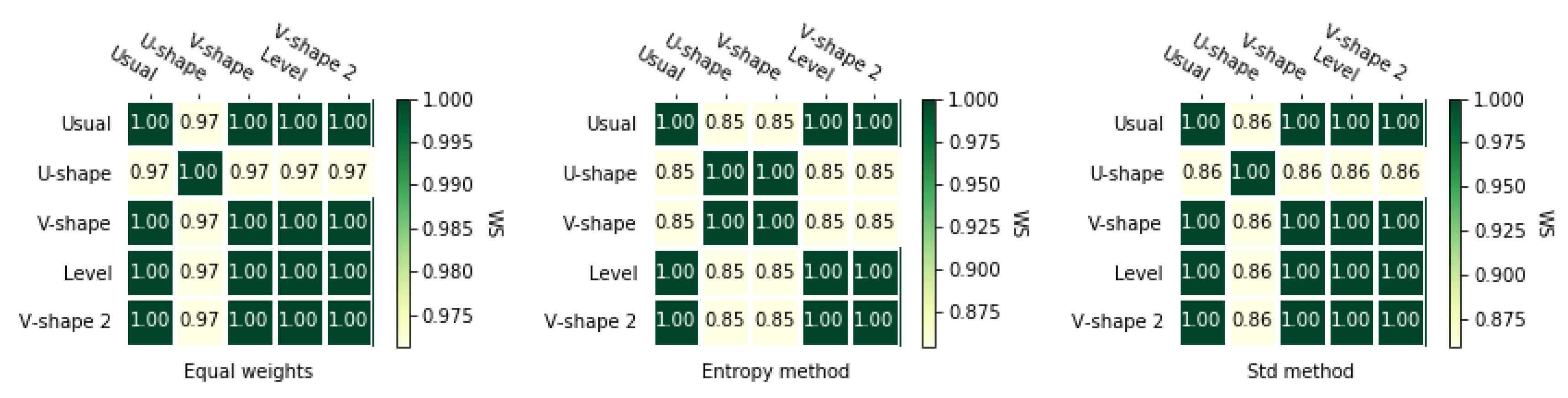
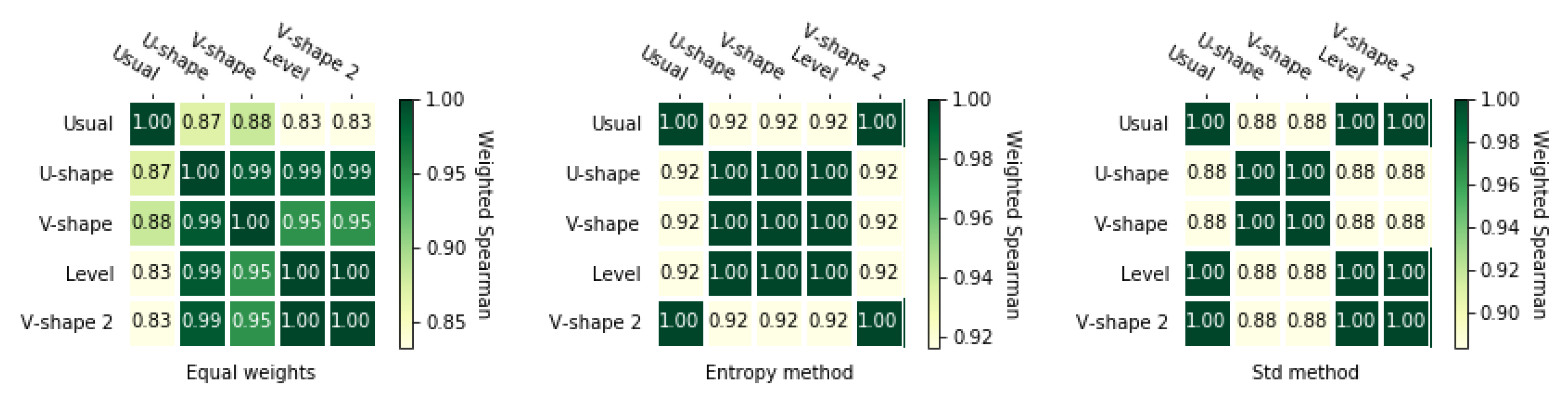
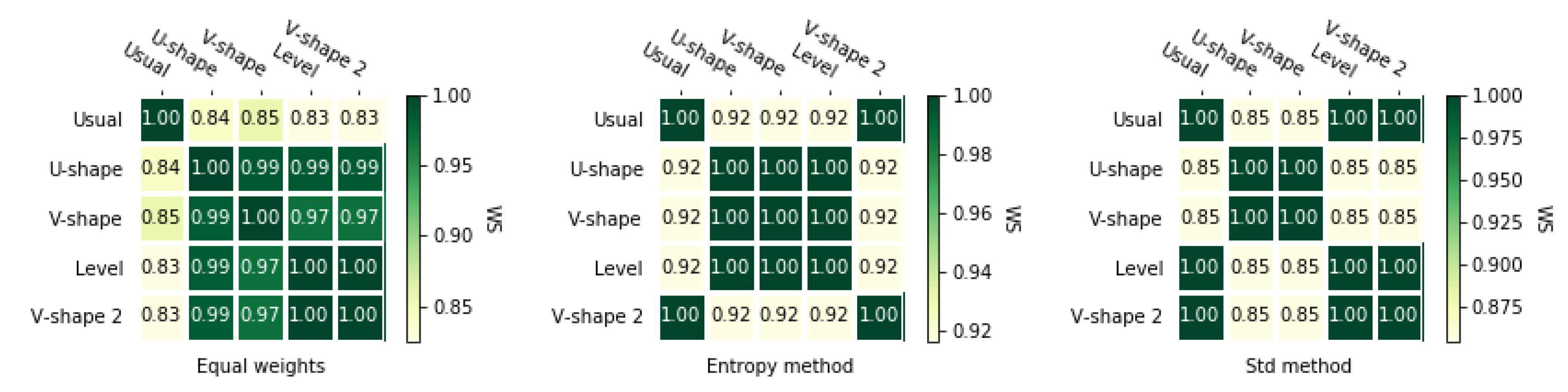
According to Figure 6 and Figure 7, entropy weighting methods give slightly less correlated rankings than the two other methods. It is noticeable that for equal weights and for std-based method ranking obtained using U-shape preference function was not the same as for other rankings.
For the second matrix, rankings obtained with the usual preference function and equal weights is quite different than other rankings which is shown in Figure A5 and Figure A6. For the entropy weighting method, we could see that the rankings obtained with the usual preference function and the v-shape 2 preference function are equal, but applying other preference functions gave us slightly different rankings. In the case of the standard weighting methods, preference functions usual, level, and v-shape 2 have equal rankings, but, as previously mentioned, they are different from the rankings obtained by other preference functions.
4.5. Different Methods
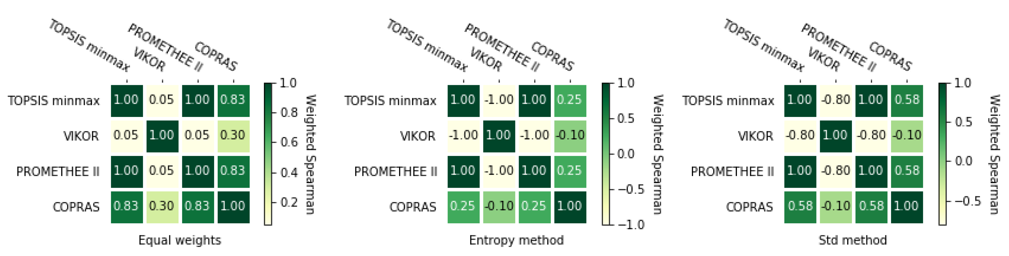
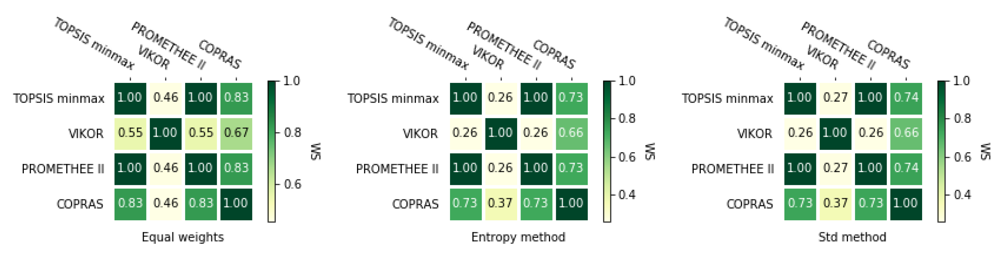
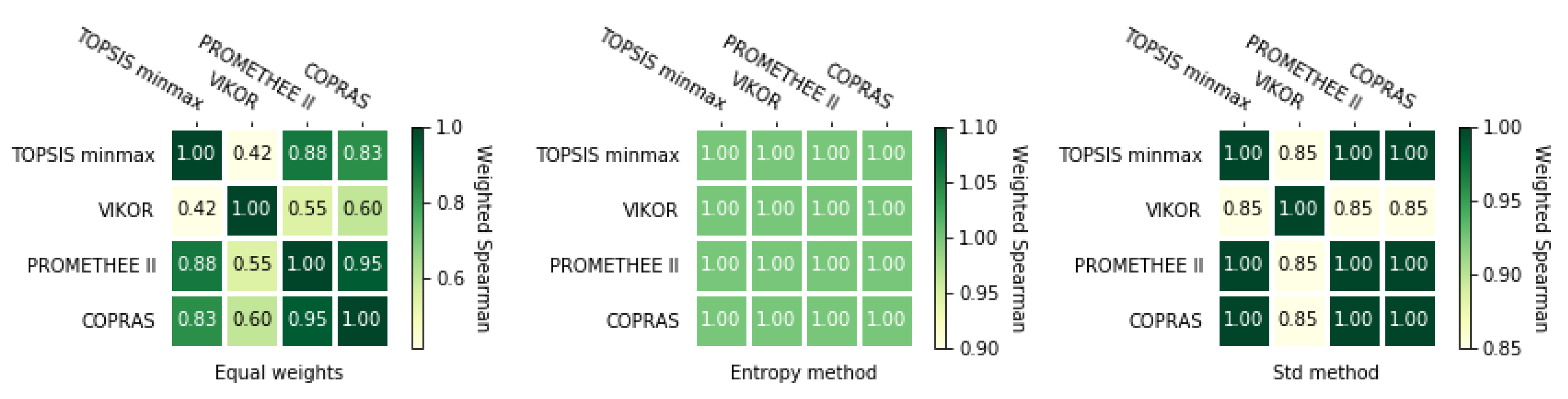
In this part, we show how different rankings could be obtained by different methods. We compare rankings obtained by TOPSIS with minmax-based normalization, VIKOR without normalization, PROMETHEE II with the usual preference function, and COPRAS. Obtained rankings for first and second matrices are shown in Table 7 and Table A5 accordingly.
Correlation heat maps are shown in Figure 8 and Figure 9. The differences between rankings in the case of the first example are the smallest. It can be seen that the ranking obtained using VIKOR and entropy weighting method is reversed to rankings obtained using TOPSIS minmax and PROMETHEE II methods. It also poorly correlated with the ranking obtained with the COPRAS method. This is also noticeable that for other two weighting methods, with the VIKOR ranking being much less correlated with other rankings.
4.6. Summary
Based on the results of the two numerical examples presented in Section 4.1, Section 4.2, Section 4.3, Section 4.4 and Section 4.5, it can be seen that the selection of the MCDA method is important for the results in the final ranking. Both numerical examples were presented to show positive and negative cases. In both samples, it can be seen that once a given method is selected, the weighing method and the normalization used in this method play a key role. The impact of parameters in the decision-making process in the discussed examples was different. Therefore, simulations should be performed in order to examine the typical similarity between the received rankings concerning a different number of alternatives. In Section 4.5, comparisons are made between methods using the most common configuration, where each of the analyzed scenarios has a huge impact on the final ranking. Therefore, simulation studies will be conducted to show the similarity of the rankings examined in the next section.
5. Results and Discussion
5.1. TOPSIS
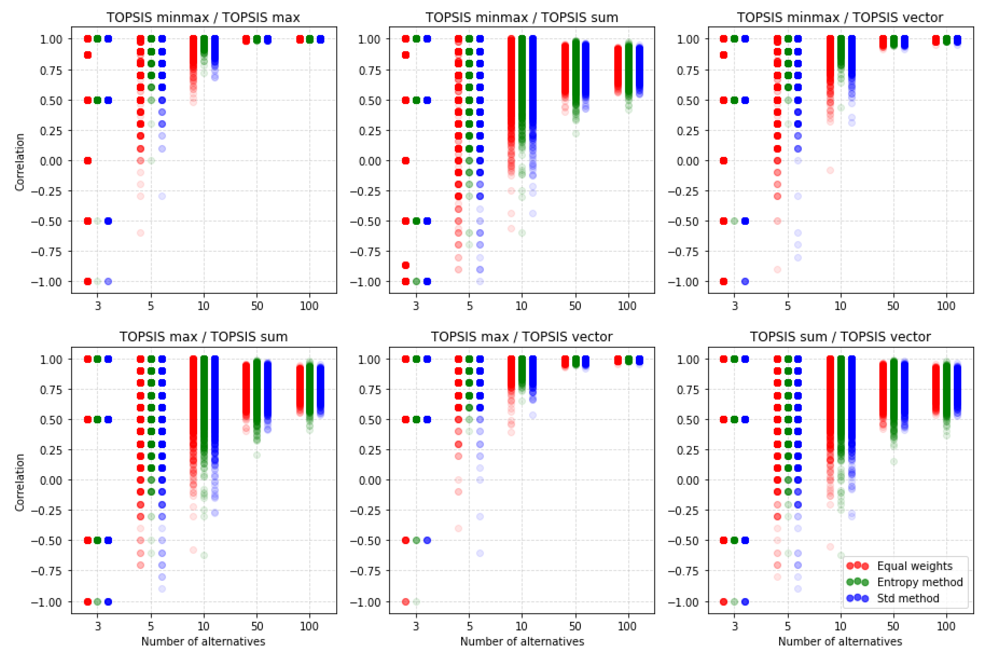
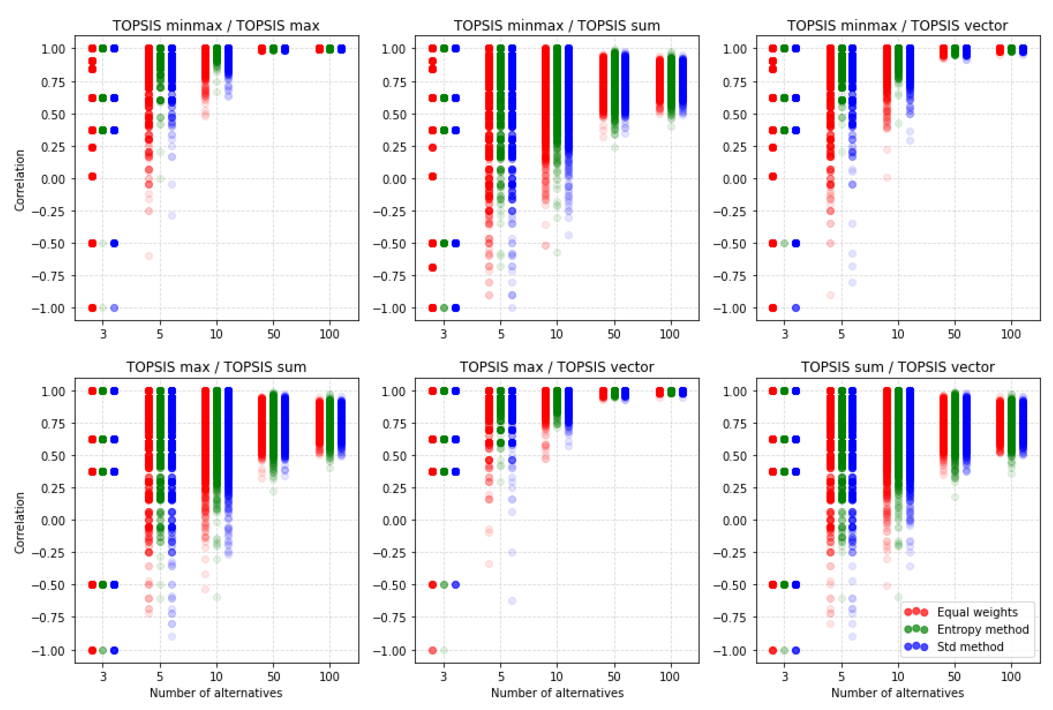
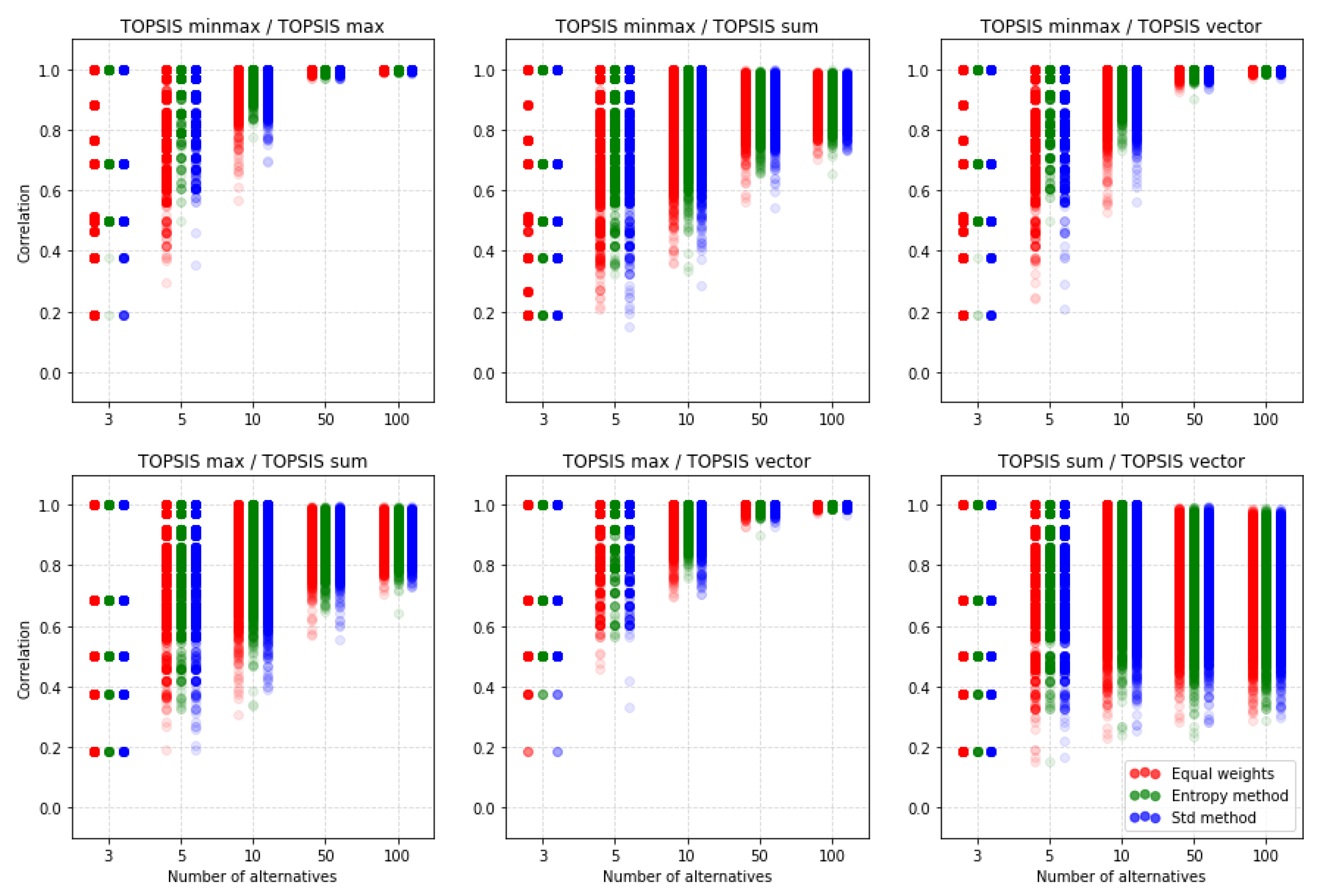
In this section, we compare TOPSIS between different normalization methods. Figure 10, Figure 11 and Figure 12 contain results of simulations. Each dot represents the correlation between two rankings for certain random matrix. The color of the dot shows which weighting method it is. For TOPSIS we compare rankings with three correlation coefficients described in Section 3.4, but other methods would be compared only using the and correlation coefficients because the Spearman correlation has some limitations. At first, we could not use the correlation for rankings where standard deviations are 0. It is frequent occurrences for the VIKOR method for decision matrices with a small number of alternatives. The second reason is that the cardinality of the Spearman correlation coefficient values set is strictly less than the cardinality of possible values sets of other two correlation coefficients. It is perfectly seen in Figure 10 for five alternative.
Figure 11 shows the correlation between rankings obtained using the TOPSIS method with different normalization methods. We have some reversed rankings for matrices with three alternatives but with a greater number of alternatives, rankings become increasingly similar. It is noticeable that for a big number of alternatives, such as 50 or 100, rankings obtained using minmax vs. max normalization, minmax vs. vector normalization, and max vs. vector normalization methods are almost perfectly correlated. It is clearly seen in Table A6, which contains mean values of this correlations. The table gives details of the average correlation values for the number of alternatives (3, 5, 10, 50, or 100) and the number of criteria (2, 3, 4, and 5). Overall, the value of reaches the lowest values for five criteria and three alternatives. The closest results are obtained for the max and minmax normalizations, but when not applying an equal distribution of criteria weights. Then, in the worst case, we get the value of the coefficient 0.897, where for the method of equal distribution of weights we get the result 0.735. Other pairs of normalizations reach, in the worst case, the correlation of 0.571. It is also visible that rankings obtained using the sum normalization method are less correlated to rankings obtained with other normalization methods. Herein we can conclude that sum normalization is performing poorly with TOPSIS compared to other normalization methods.
On Figure 12, we see similar results to . Rankings obtained using sum normalization are less correlated with other rankings. It is noticeable that according to the similarity coefficient, there are more poorly correlated rankings for the sum vs. vector normalization methods case than for correlation. A problem of interpretation may be that both coefficients have a different domain. Nevertheless, this is the only case where the number of alternatives is increasing and there is no improvement in the similarity of the rankings obtained. The detailed data in Table A7 also confirm this. It may also come as a big surprise that the choice of the weighting method is not so important. Relatively similar results are obtained regardless of the method used.
In general, it follows that with a small number of alternatives that do not exceed 10 decision-making options, the rankings may vary considerably depending on the normalization chosen. Thus, this shows that a problem as important as the choice of the method of weighting is the choice of the method used to normalize the input data. For larger groups of alternatives, the differences are also significant, although a smaller difference can be expected. The analysis of the data in Table A6 and Table A7 shows that the increase in the complexity of the problem, understood as an increase in the number of criteria, practically always results in the decrease in similarity between the results obtained as a result of different normalizations applied.
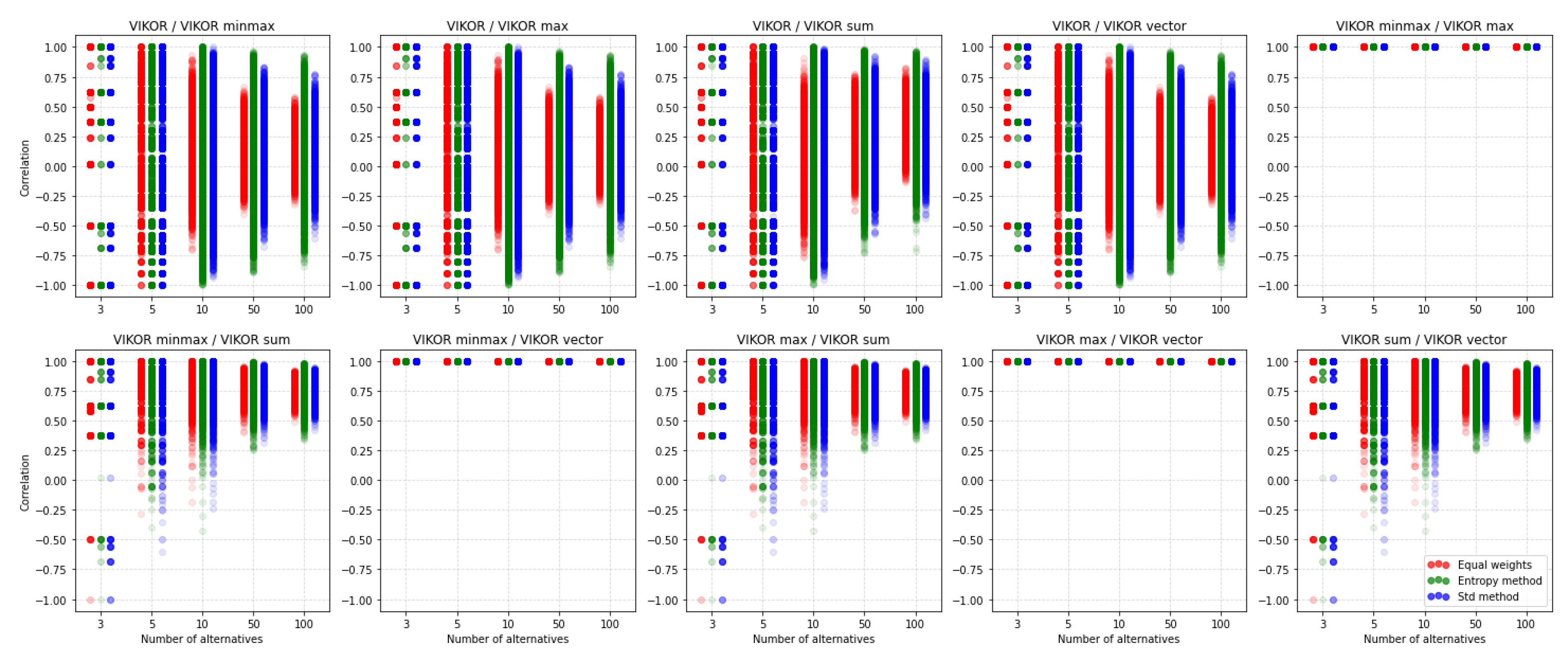
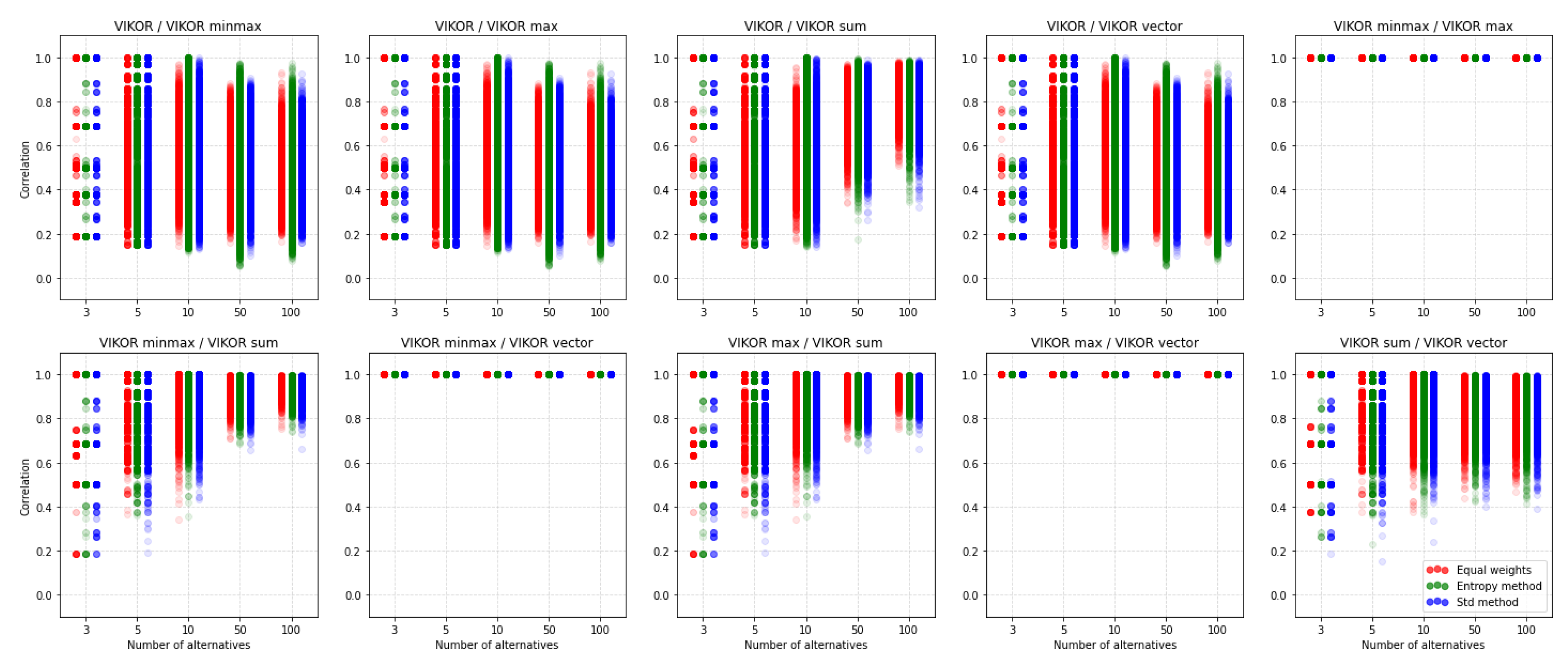
5.2. VIKOR
As mentioned previously, we would use only and correlation coefficients for the following comparisons. Figure 13 shows correlation between rankings obtained using VIKOR with different normalization and without normalization. It is clearly seen that VIKOR without normalization is poorly correlated to VIKOR when normalization is applied. In Table A8, we could see that mean values of the correlation values for VIKOR without normalization with cases where normalization was applied is around 0. It is also noticeable that VIKOR with minmax, max, and vector normalization gives very similar rankings.
This is similar to the TOPSIS method, where sum normalization has less similar rankings than other methods. Interestingly, correlations of rankings in the case of VIKOR without normalization vs. VIKOR with any normalization have a mean around zero, but rankings obtained with equal weight have less variance. In this case, less variability may be of concern, as it means that it is not possible to get rankings that are compatible. In addition to the three exceptions mentioned earlier, it should be noted that the choice of normalization has a significantly stronger impact on the similarity of rankings than in the TOPSIS method.
We can observe a similar situation on Figure 14, where similar coefficient values are presented. It confirms the results obtained using correlation coefficient: Rankings obtained using VIKOR without normalization is less correlated with rankings obtained using VIKOR with normalization than other rankings correlated between themselves. It is also noticeable that in the sum vs. vector normalization methods case, the similarity coefficient values are also visibly smaller, as it was for TOPSIS. Therefore, we can conclude that rankings obtained using the sum and vector normalization method usually should be quite different.
A detailed analysis of the results of mean values of (Table A8) and mean (Table A9) show that the mean significance of similarities is significantly lower than in the TOPSIS method. Besides, the dependence of the change in the values of both coefficients in the tables is more random and more challenging to predict. Nevertheless, it means that the final result of the ranking is significant whether or not we apply the method with or without normalization, and which normalization we apply. Again, the influence of the selection of the method of criteria weighting was not as significant as one might expect. Generally, the proof is shown here that standardization can have a considerable impact on the final result.
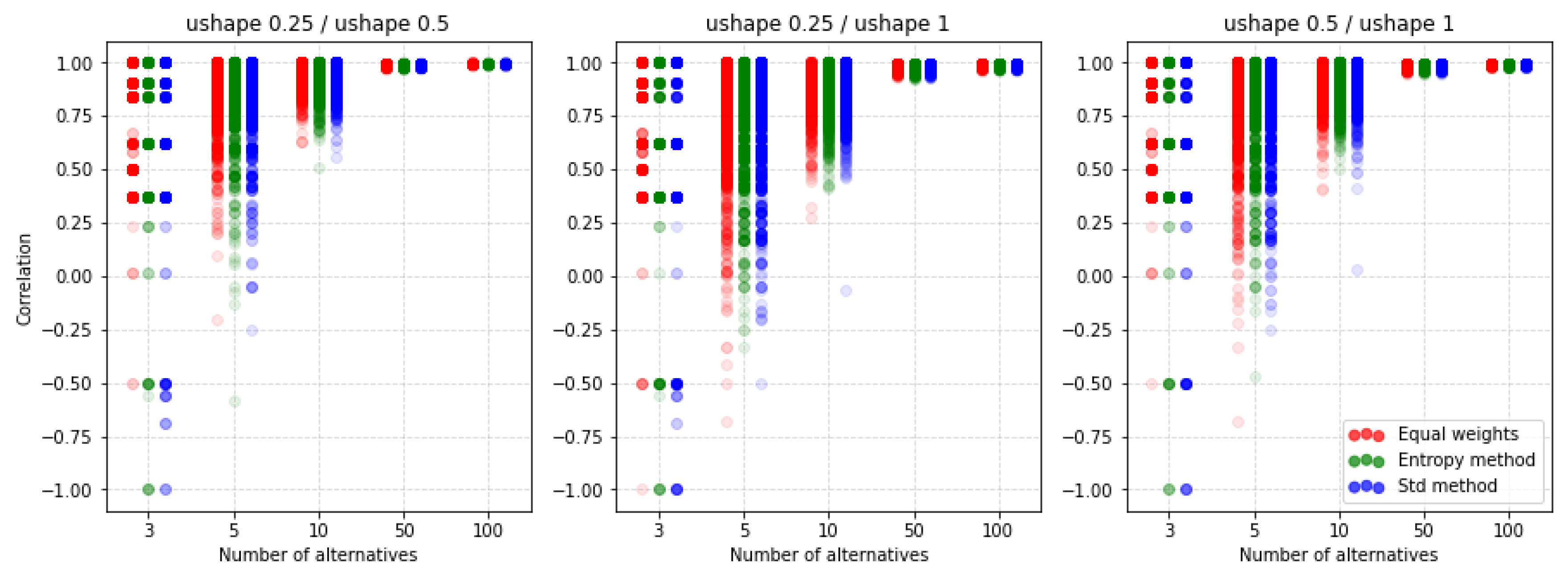
5.3. PROMETHEE II
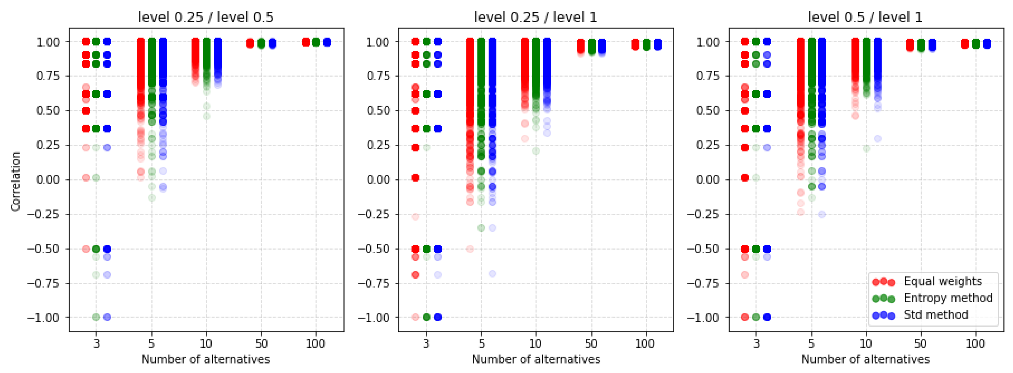
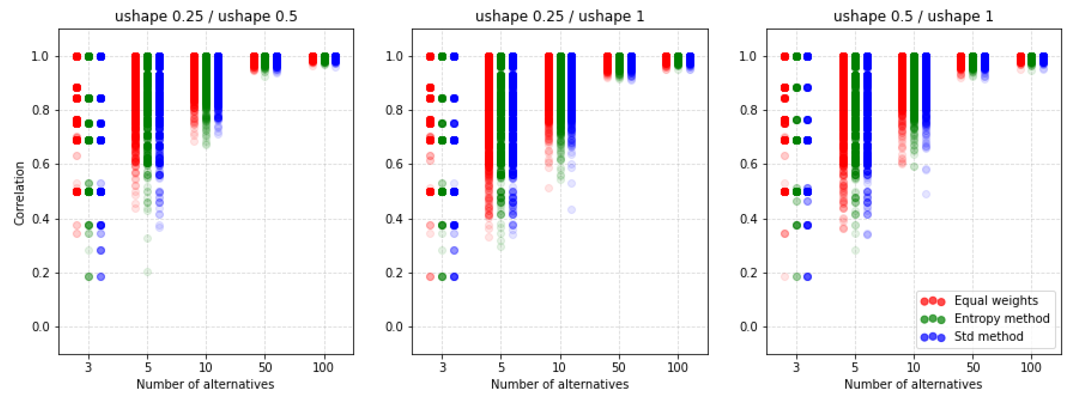
For PROMETHEE II, the normalization of the decision matrix does not apply. That is why this section will analyze receiving the rankings with different values of parameters p, q, and preference function. Figure 15 shows the results of the factor for the U-shape preference function concerning different techniques of criteria weighting. The values p and q are calculated automatically and we only scale them. The differences between the individual rankings are very similar. If we analyze up to 10 alternatives, using any scaling value, we get significantly different results. As the number of alternatives increases, the spread of possible correlation values decreases. However, when analyzing the values contained in Table A10 and Table A11 we see that the average values indicate a much smaller impact than in the case of the selection of standardization methods in the two previous MCDA methods.
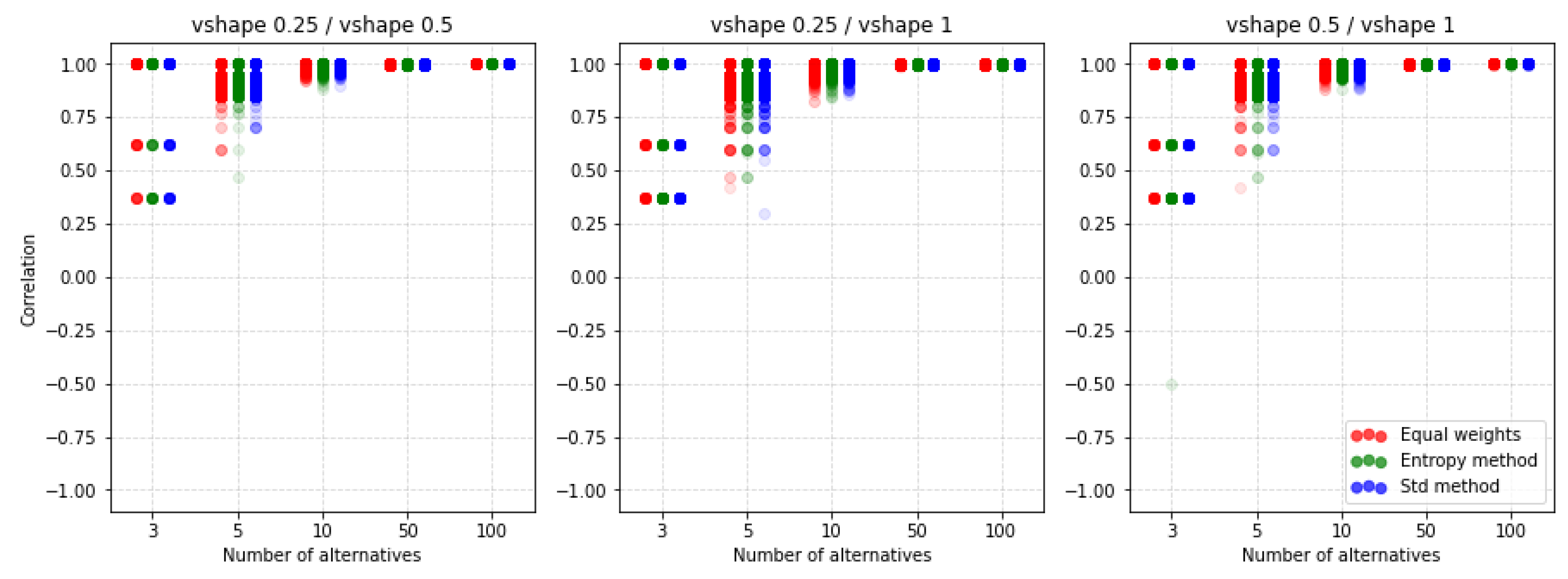
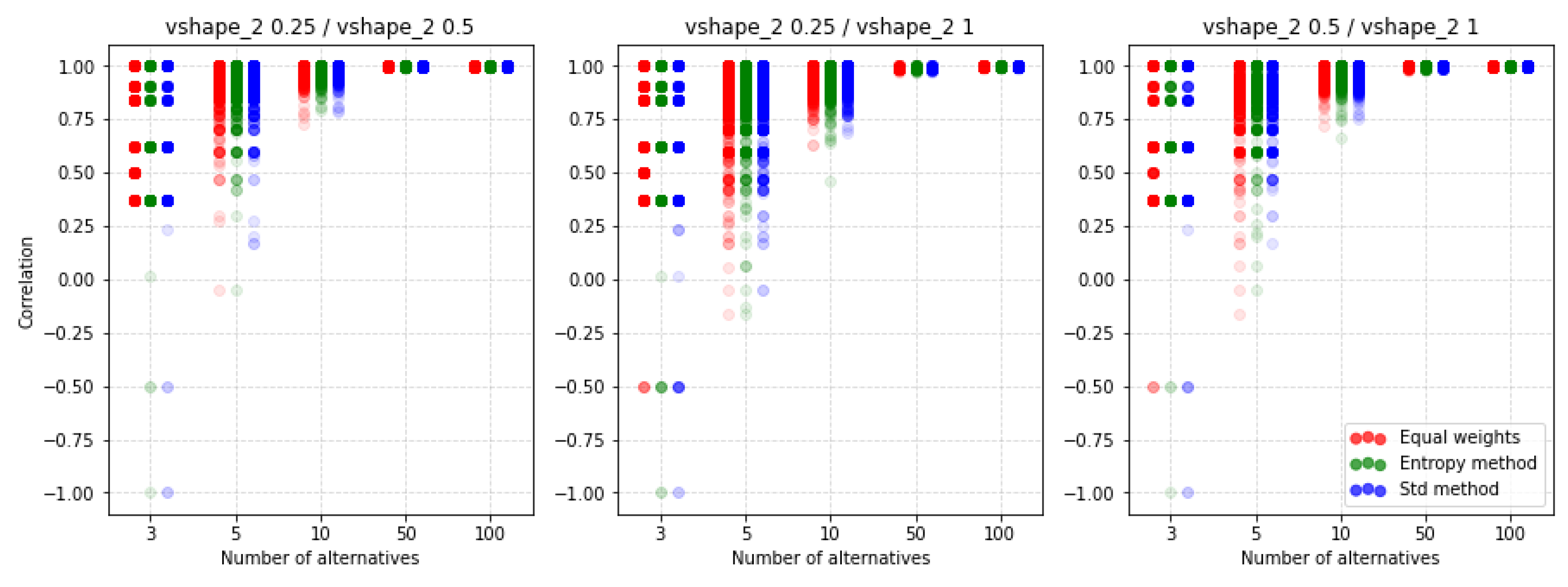
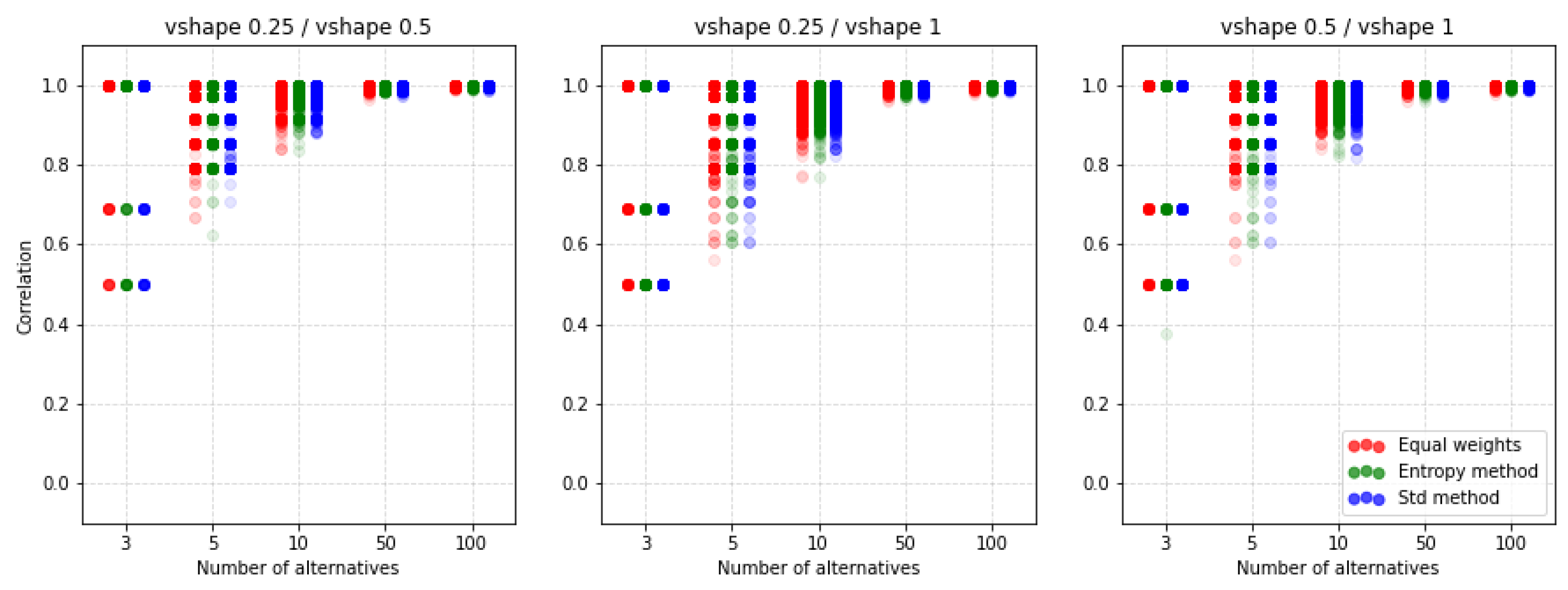
For comparison, we present Figure 16 where another preference function is shown but also for the ratio. It turns out that by choosing the V-shape preference function instead of the U-shape we get more of a similarity of results. Again, it turns out that the methods of weighting do not have such a significant impact on the similarity results obtained.
An important observation is that despite the lack of possibilities to normalize input data, there are still differences depending on the selected parameters and functions of preferences. The other two preference functions for the ratio are shown in Figure A9 and Figure A10. The results also indicate a similar level of similarity between the rankings. The coefficient for the corresponding cases is shown in Figure A11, Figure A12, Figure A13 and Figure A14. Both coefficients indicate the same nature of the influence of the applied parameters on the similarity of rankings. To sum up, in all the discussed cases, we see significant differences between the rankings obtained. Thus, not only normalization but other parameters are important for the results obtained and it is always necessary to make an in-depth analysis by selecting a specific method and assumptions, i.e., such as normalization, etc.
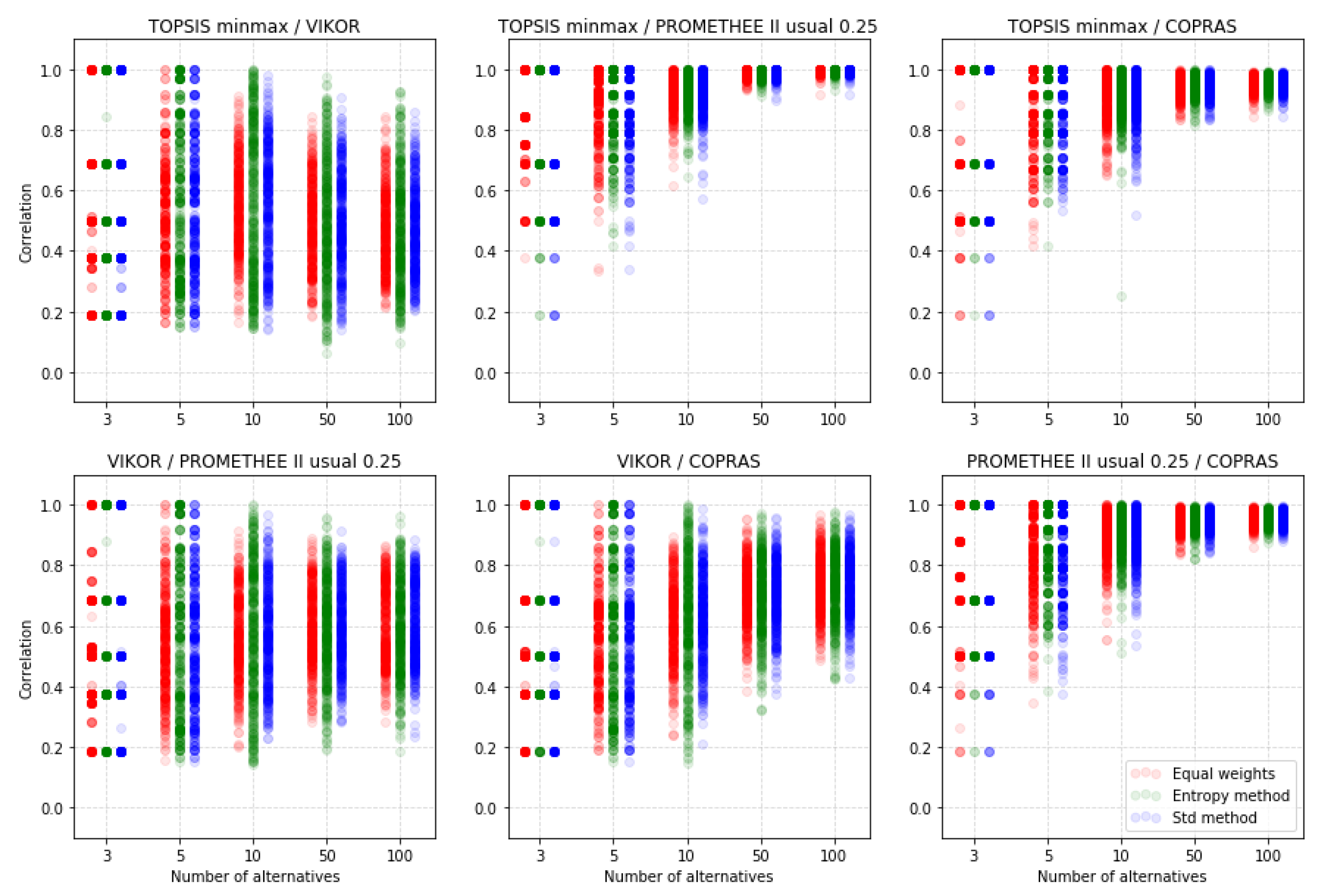
5.4. Comparison of the MCDA Methods
Figure 17 shows how much correlated rankings obtained by four different methods could be: TOPSIS with minmax normalization, VIKOR without normalization, PROMETHEE II with usual preference function, and COPRAS. We can see that VIKOR has quite different rankings in comparison to other methods.
Table A12 shows that the mean values of the correlation between VIKOR rankings and other methods’ rankings are around zero. It is also noticeable that for cases VIKOR vs. other method correlation for rankings obtained using equal weights has a smaller variance in comparison to the other two weighting methods. Next, we could see that mostly correlated rankings could be obtained with TOPSIS minmax and PROMETHEE II usual methods. The comparisons between TOPSIS minmax vs. COPRAS and PROMETHEE II usual vs. COPRAS look quite similar and this methods’ rankings are less correlated between themselves than TOPSIS minmax and PROMETHEE II usual methods’ rankings.
The general situation is quite similar for correlation coefficient, as it shows Figure 18. The rankings obtained by VIKOR are far less correlated to rankings obtained using the other three methods than these rankings between themselves. Similarly to , points that rankings obtained using TOPSIS minmax and PROMETHEE II usual methods have a strong correlation between themselves. Rankings obtained by TOPSIS minmax, COPRAS, and PROMETHEE II with the usual preference function are slightly less correlated. However, correlations between them are stronger than in the case of VIKOR vs. other methods.
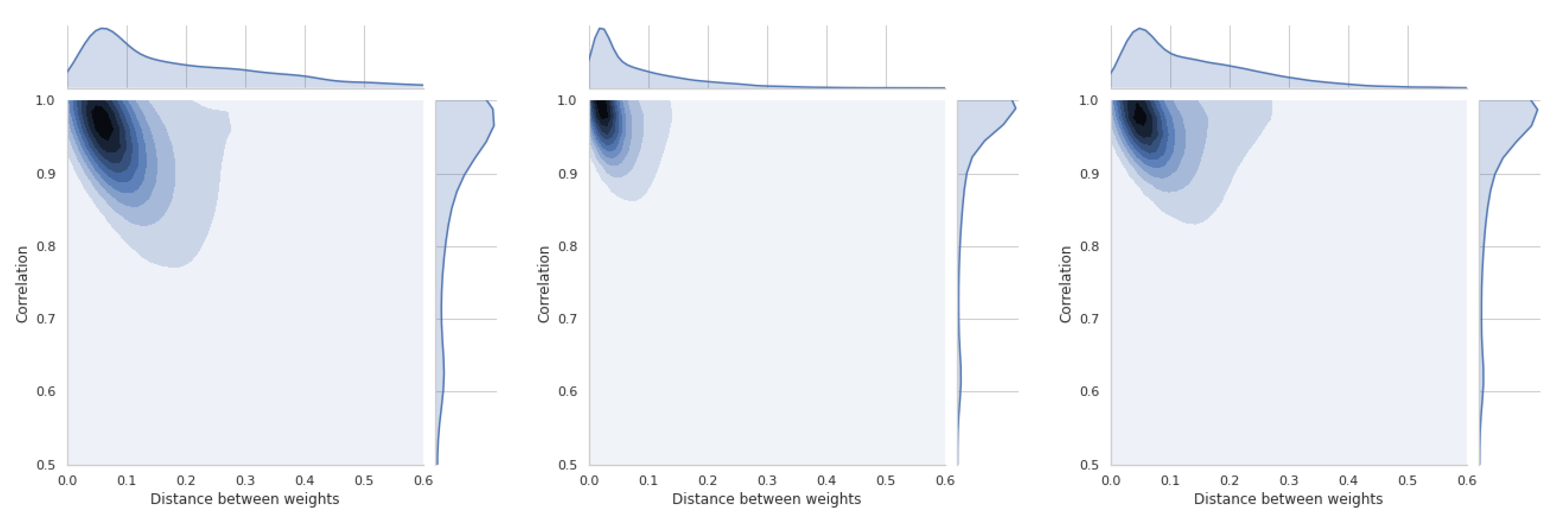
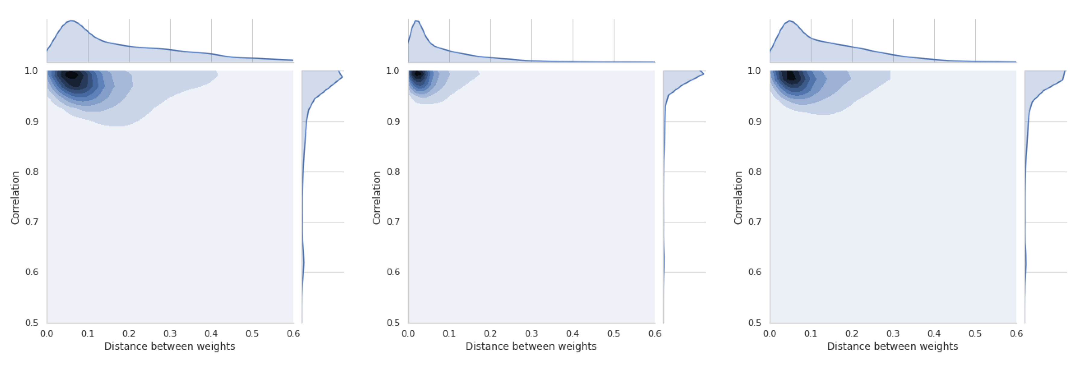
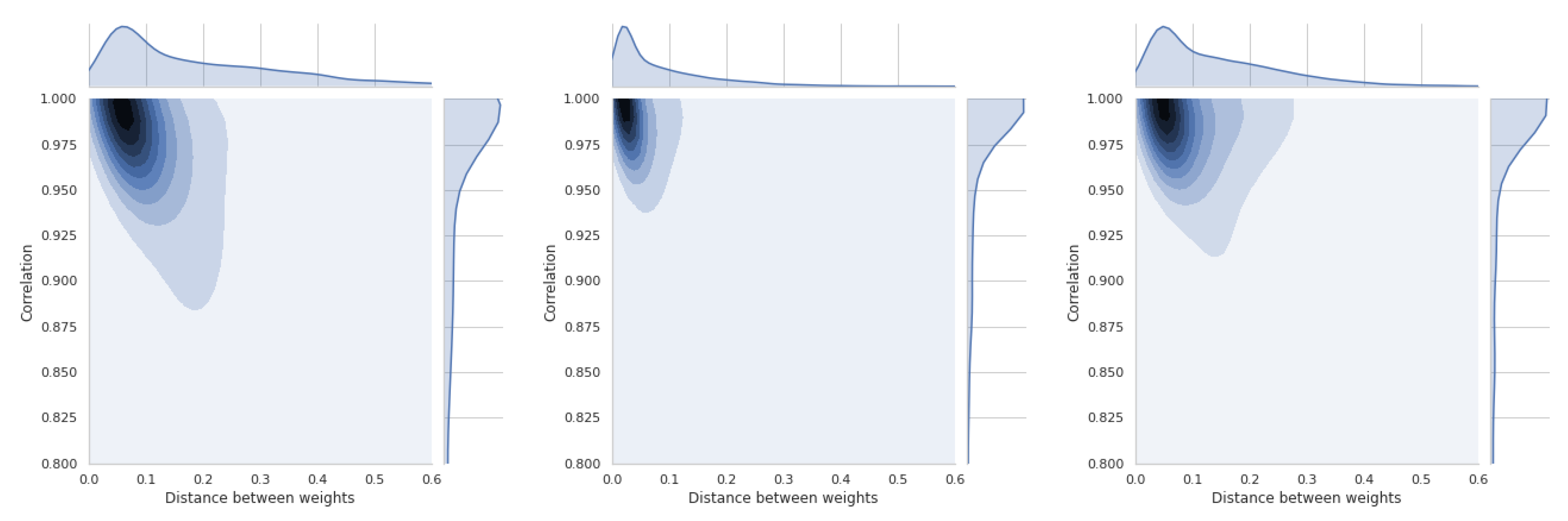
5.5. Dependence of Ranking Similarity Coefficients on the Distance between Weight Vectors
The last section is devoted to a short presentation of distance distributions between weight vectors and similarity coefficients. All these distributions are asymmetric and will be briefly discussed for each of the four methods used. Thus, Figure 19 shows the relations between coefficient and TOPSIS method. The smallest difference in the distance between the vectors of weights is between the equal weights and those obtained by the std method. These values refer to all simulations that have been performed and cannot be generalized to the whole space. In Figure A15, there is a distribution for the coefficient, which confirms that there is a moderate relation between the distance of weight vectors and the similarity coefficient of obtained rankings.
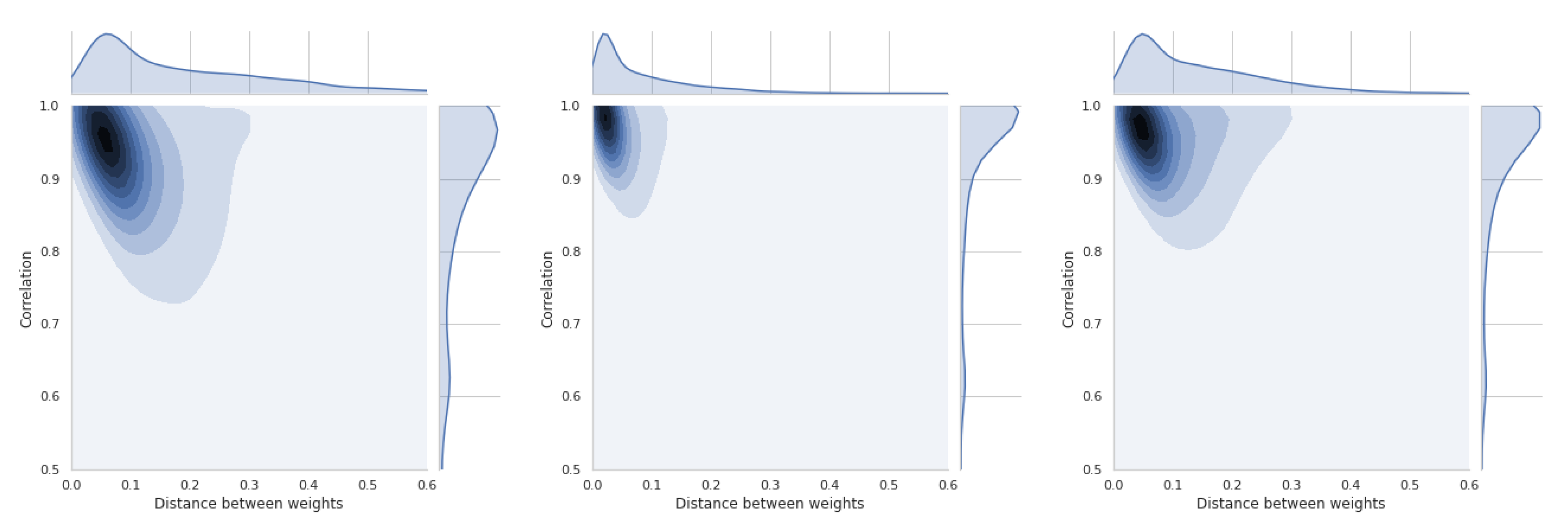
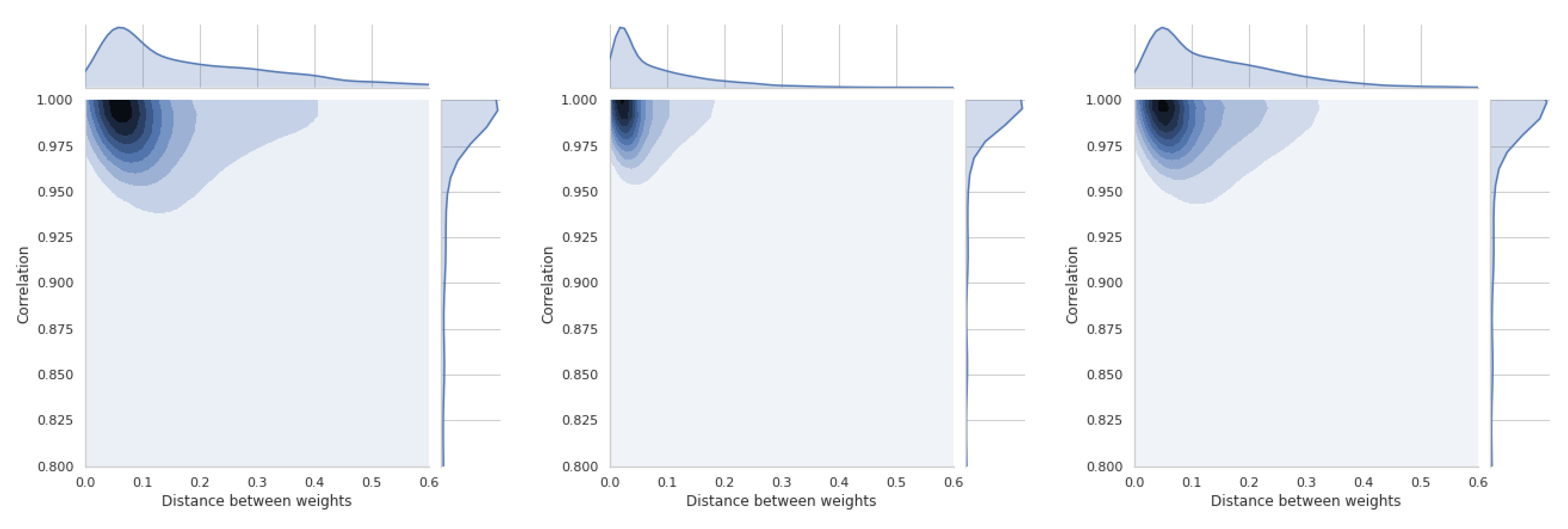
In Figure 20, the results of the VIKOR method are presented. The distribution of similarity coefficient is very similar to the distribution obtained for the TOPSIS method. Distance distributions between vectors of respective methods are the same for all presented graphs. Figure A16 shows the relationships for the VIKOR method and WS coefficient.
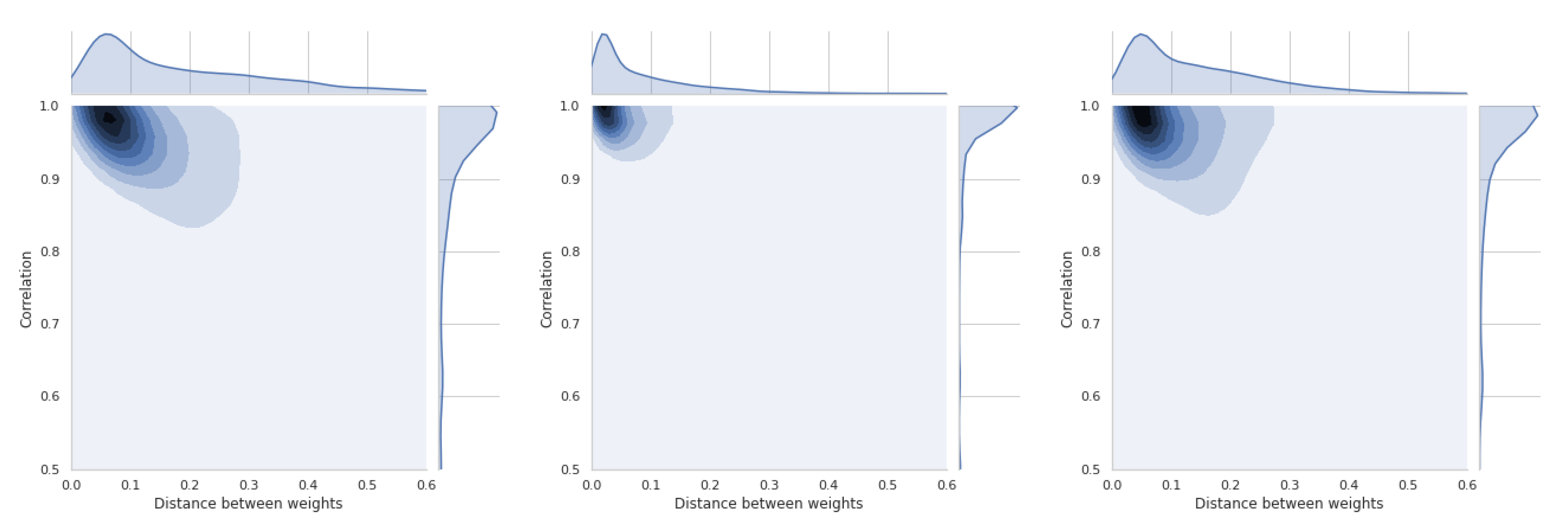
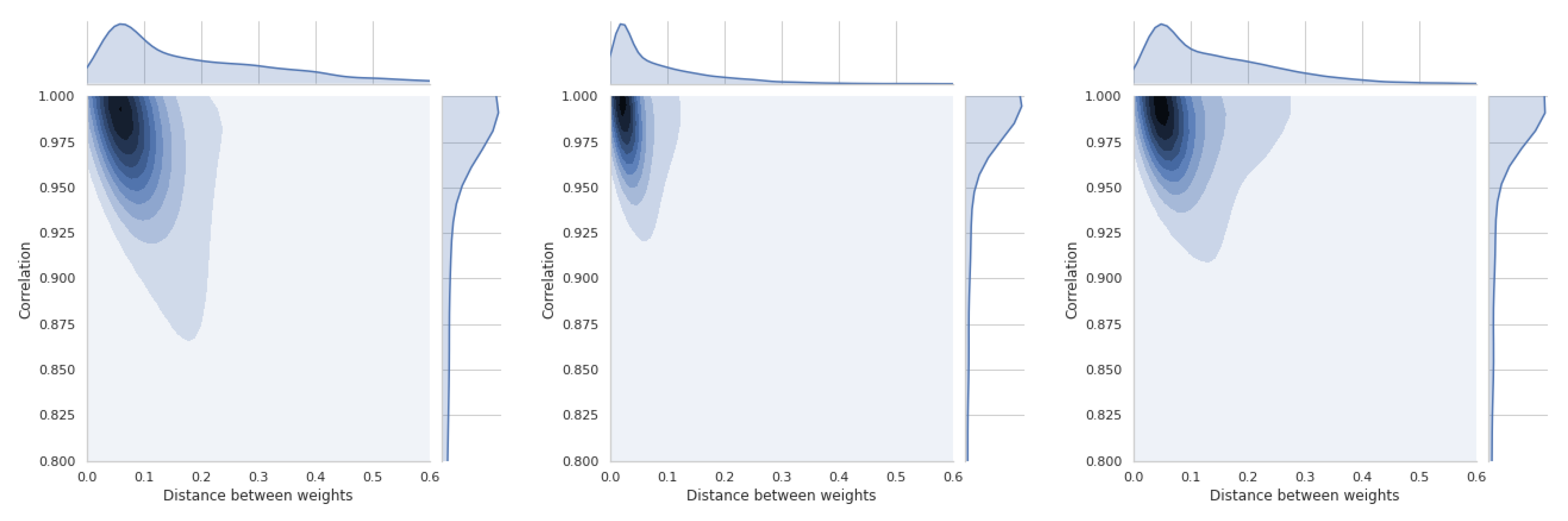
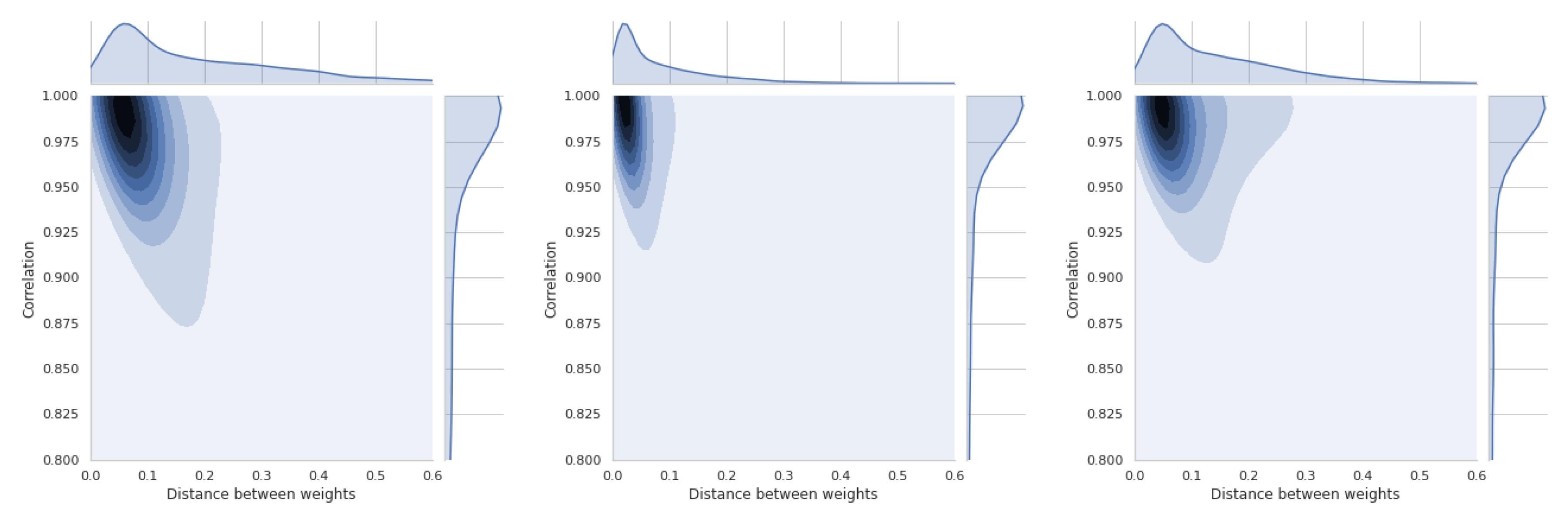
Using the PROMETHEE II method (usual), we can observe changes in the relation which is presented in Figure 21 and Figure A17. This means that the use of different weights in the presented simulation was less important in the PROMETHEE II method than in the TOPSIS or VIKOR method. The distance between the scale vectors was the least important in the COPRAS method, the results of which are presented in Figure 22 and Figure A18.
These results are important preliminary research on whether the weights and their differences always have a important influence on the compliance of the obtained rankings. TOPSIS and VIKOR have the highest sensitivity in the presented experiment, and COPRAS has the lowest sensitivity.
6. Conclusions
The results of the conducted research indicate that when choosing the MCDA method, not only the method itself but also the method of normalization and other parameters should be carefully selected. Almost every combination of the method and its parameters may bring us different results. In our study, we have checked how much influence these decisions can have on the ranking of the decision problem. As it turns out, it may weigh not only the correct identification of the best alternative but also the whole ranking.
For the TOPSIS method, rankings obtained using minmax, max, and vector normalization method could be quite similar, especially for the big number of alternatives. In this case, equal weights performed worse than entropy or standard deviation method. Furthermore, with these normalization methods, correlation of rankings had a smaller variance when the entropy weighting method was used. For VIKOR, rankings obtained using any normalization methods could be even reversed in comparison to rankings obtained using VIKOR without normalization. Thus, although it was not necessary to apply normalization when using VIKOR, applying one could be noticeable to improve rankings and the overall performance of the method. Equal weights performed better with VIKOR. The PROMETHEE II method, despite the lack of use of normalization, returned quite different results depending on the set of parameters used and it clearly showed that the choice of the method and its configuration for the decision-making problem was important and should be the subject of further benchmarking. In four different method comparison, rankings obtained using VIKOR without normalization were very different from rankings obtained by other methods. Some equal rankings for the small number of alternatives was achieved. However, for a greater number of alternatives, correlations between VIKOR’s rankings and other methods rankings had oscillated around zero, which means that there was no correlation between these rankings. Most similar rankings were obtained using TOPSIS minmax and PROMETHEE II usual methods. In this case, equal weighting methods performed slightly better. This proves that it is worthwhile to research in order to develop reliable and generalized benchmarks.
The direction of future work should be focused on the development of an algorithm for estimation of accuracy for multi-criteria decision analysis method and estimating the accuracy of selected multi-criteria decision-making methods. However, special attention should be paid to the family of fuzzy set-based MCDA methods and group decision making methods as well. Another challenge is to create a method that, based on the results of the benchmarks, will be able to recommend a proper solution.
Author Contributions
Conceptualization, A.S. and W.S.; methodology, A.S. and W.S.; software, A.S.; validation, A.S., J.W., and W.S.; formal analysis, A.S., J.W., and W.S.; investigation, A.S. and W.S.; resources, A.S.; data curation, A.S.; writing—original draft preparation, A.S. and W.S.; writing—review and editing, A.S., J.W., and W.S.; visualization, A.S. and W.S.; supervision, W.S.; project administration, W.S.; funding acquisition, W.S. All authors have read and agreed to the published version of the manuscript.
Funding
The work was supported by the National Science Centre, Decision number UMO-2018/29/B/HS4/02725.
Acknowledgments
The authors would like to thank the editor and the anonymous reviewers, whose insightful comments and constructive suggestions helped us to significantly improve the quality of this paper.
Conflicts of Interest
The authors declare no conflict of interest.
Abbreviations
The following abbreviations are used in this manuscript:
| TOPSIS | Technique for Order of Preference by Similarity to Ideal Solution |
| VIKOR | VlseKriterijumska Optimizacija I Kompromisno Resenje (Serbian) |
| COPRAS | Complex Proportional Assessment |
| PROMETHEE | Preference Ranking Organization Method for Enrichment of Evaluation |
| MCDA | Multi Criteria Decision Analysis |
| MCDM | Multi Criteria Decision Making |
| PIS | Positive Ideal Solution |
| NIS | Negative ideal Solution |
| SD | Standard Deviation |
Appendix A. Figures
Figure A1.
correlations heat map for TOPSIS with different normalization methods (matrix 2).

Figure A2.
correlations heat map for TOPSIS with different normalization methods (matrix 2).

Figure A3.
correlations heat map for VIKOR with different normalization methods (matrix 2).

Figure A4.
correlations heat map for VIKOR with different normalization methods (matrix 2).

Figure A5.
correlations heat map for PROMETHEE II with different preference functions (matrix 2).

Figure A6.
correlations heat map for PROMETHEE II with different preference functions (matrix 2).

Figure A7.
correlations heat map for PROMETHEE II with different preference functions (matrix 2).

Figure A8.
correlations heat map for PROMETHEE II with different preference functions (matrix 2).

Figure A9.
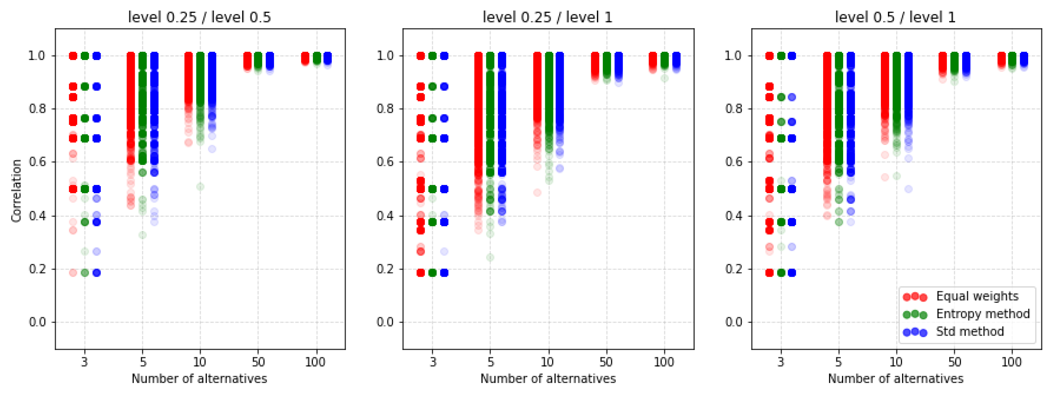
Comparison of the similarity coefficient for the PROMETHEE II method with level preference function and different k values.
Figure A9.
Comparison of the similarity coefficient for the PROMETHEE II method with level preference function and different k values.

Figure A10.
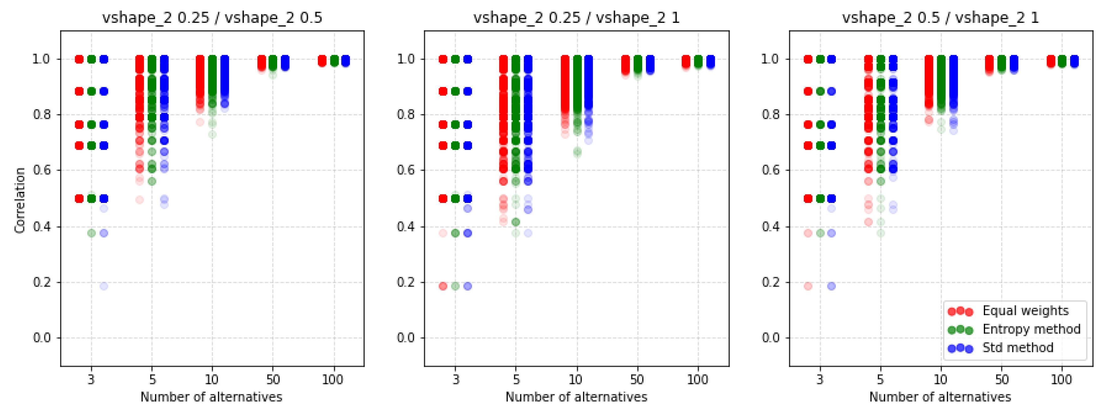
Comparison of the similarity coefficient for the PROMETHEE II method with V-shape 2 preference function and different k values.
Figure A10.
Comparison of the similarity coefficient for the PROMETHEE II method with V-shape 2 preference function and different k values.

Figure A11.
Comparison of the similarity coefficient for the PROMETHEE II method with U-shape preference function and different k values.
Figure A11.
Comparison of the similarity coefficient for the PROMETHEE II method with U-shape preference function and different k values.

Figure A12.
Comparison of the similarity coefficient for the PROMETHEE II method with V-shape preference function and different k values.
Figure A12.
Comparison of the similarity coefficient for the PROMETHEE II method with V-shape preference function and different k values.

Figure A13.
Comparison of the similarity coefficient for the PROMETHEE II method with level preference function and different k values.
Figure A13.
Comparison of the similarity coefficient for the PROMETHEE II method with level preference function and different k values.

Figure A14.
Comparison of the similarity coefficient for the PROMETHEE II method with V-shape 2 preference function and different k values.
Figure A14.
Comparison of the similarity coefficient for the PROMETHEE II method with V-shape 2 preference function and different k values.

Figure A15.
Relationship between the euclidean distance of weights and similarity coefficient for rankings obtained by the TOPSIS method with different weighting methods, where (left) equal/entropy, (center) equal/std, and (right) std/entropy.
Figure A15.
Relationship between the euclidean distance of weights and similarity coefficient for rankings obtained by the TOPSIS method with different weighting methods, where (left) equal/entropy, (center) equal/std, and (right) std/entropy.

Figure A16.
Relationship between the euclidean distance of weights and similarity coefficient for rankings obtained by the VIKOR method with different weighting methods, where (left) equal/entropy, (center) equal/std, and (right) std/entropy.
Figure A16.
Relationship between the euclidean distance of weights and similarity coefficient for rankings obtained by the VIKOR method with different weighting methods, where (left) equal/entropy, (center) equal/std, and (right) std/entropy.

Figure A17.
Relationship between the euclidean distance of weights and similarity coefficient for rankings obtained by the PROMETHEE II (usual) method with different weighting methods, where (left) equal/entropy, (center) equal/std, and (right) std/entropy.
Figure A17.
Relationship between the euclidean distance of weights and similarity coefficient for rankings obtained by the PROMETHEE II (usual) method with different weighting methods, where (left) equal/entropy, (center) equal/std, and (right) std/entropy.

Figure A18.
Relationship between the euclidean distance of weights and similarity coefficient for rankings obtained by the COPRAS method with different weighting methods, where (left) equal/entropy, (center) equal/std, and (right) std/entropy.
Figure A18.
Relationship between the euclidean distance of weights and similarity coefficient for rankings obtained by the COPRAS method with different weighting methods, where (left) equal/entropy, (center) equal/std, and (right) std/entropy.

Appendix B. Tables

Table A1.
The second example decision matrix with three different criteria weighting vectors.
| 0.947 | 0.957 | 0.275 | |
| 0.018 | 0.631 | 0.581 | |
| 0.565 | 0.295 | 0.701 | |
| 0.423 | 0.602 | 0.509 | |
| 0.664 | 0.637 | 0.786 | |
| 0.333 | 0.333 | 0.333 | |
| 0.678 | 0.172 | 0.151 | |
| 0.442 | 0.303 | 0.255 |
Table A2.
TOPSIS rankings for matrix 2: (a) Equal weights, (b) entropy method, and (c) std method.
| Minmax | Max | Sum | Vector | ||||||||||||
|---|---|---|---|---|---|---|---|---|---|---|---|---|---|---|---|
| (a) | (b) | (c) | (a) | (b) | (c) | (a) | (b) | (c) | (a) | (b) | (c) | ||||
| 1 | 1 | 1 | 1 | 1 | 1 | 1 | 1 | 1 | 1 | 1 | 1 | ||||
| 4 | 5 | 5 | 5 | 5 | 5 | 5 | 5 | 5 | 5 | 5 | 5 | ||||
| 5 | 3 | 4 | 4 | 3 | 3 | 4 | 3 | 3 | 4 | 3 | 3 | ||||
| 2 | 4 | 3 | 3 | 4 | 4 | 3 | 4 | 4 | 3 | 4 | 4 | ||||
| 3 | 2 | 2 | 2 | 2 | 2 | 2 | 2 | 2 | 2 | 2 | 2 | ||||
Table A3.
VIKOR rankings for matrix 2: (a) Equal weights, (b) entropy method, and (c) std method.
| None | Minmax | Max | Sum | Vector | |||||||||||||||
|---|---|---|---|---|---|---|---|---|---|---|---|---|---|---|---|---|---|---|---|
| (a) | (b) | (c) | (a) | (b) | (c) | (a) | (b) | (c) | (a) | (b) | (c) | (a) | (b) | (c) | |||||
| 3 | 1 | 2 | 1 | 1 | 1 | 1 | 1 | 1 | 1 | 1 | 1 | 1 | 1 | 1 | |||||
| 5 | 5 | 5 | 4 | 5 | 5 | 4 | 5 | 5 | 4 | 5 | 5 | 4 | 5 | 5 | |||||
| 4 | 3 | 4 | 5 | 3 | 4 | 5 | 3 | 4 | 5 | 3 | 4 | 5 | 3 | 4 | |||||
| 2 | 4 | 3 | 2 | 4 | 2 | 2 | 4 | 2 | 2 | 4 | 3 | 2 | 4 | 2 | |||||
| 1 | 2 | 1 | 3 | 2 | 3 | 3 | 2 | 3 | 3 | 2 | 2 | 3 | 2 | 3 | |||||
Table A4.
PROMETHEE II rankings for matrix 2: (a) Equal weights, (b) entropy method, and (c) std method.
Table A4.
PROMETHEE II rankings for matrix 2: (a) Equal weights, (b) entropy method, and (c) std method.
| Usual | U-Shape | V-Shape | Level | V-Shape 2 | |||||||||||||||
|---|---|---|---|---|---|---|---|---|---|---|---|---|---|---|---|---|---|---|---|
| (a) | (b) | (c) | (a) | (b) | (c) | (a) | (b) | (c) | (a) | (b) | (c) | (a) | (b) | (c) | |||||
| 1 | 1 | 1 | 1 | 1 | 1 | 1 | 1 | 1 | 1 | 1 | 1 | 1 | 1 | 1 | |||||
| 4 | 5 | 5 | 4 | 5 | 5 | 4 | 5 | 5 | 5 | 5 | 5 | 5 | 5 | 5 | |||||
| 5 | 3 | 4 | 4 | 4 | 4 | 5 | 4 | 4 | 4 | 4 | 4 | 4 | 3 | 4 | |||||
| 3 | 4 | 3 | 2 | 3 | 2 | 2 | 3 | 2 | 2 | 3 | 3 | 2 | 4 | 3 | |||||
| 2 | 2 | 2 | 3 | 2 | 3 | 3 | 2 | 3 | 3 | 2 | 2 | 3 | 2 | 2 | |||||
Table A5.
Rankings obtained with different MCDA methods for matrix 2: (a) Equal weights, (b) entropy method, and (c) std method.
Table A5.
Rankings obtained with different MCDA methods for matrix 2: (a) Equal weights, (b) entropy method, and (c) std method.
| TOPSIS | VIKOR | PROM. II | COPRAS | ||||||||||||
|---|---|---|---|---|---|---|---|---|---|---|---|---|---|---|---|
| (a) | (b) | (c) | (a) | (b) | (c) | (a) | (b) | (c) | (a) | (b) | (c) | ||||
| 1 | 1 | 1 | 3 | 1 | 2 | 1 | 1 | 1 | 1 | 1 | 1 | ||||
| 4 | 5 | 5 | 5 | 5 | 5 | 4 | 5 | 5 | 5 | 5 | 5 | ||||
| 5 | 3 | 4 | 4 | 3 | 4 | 5 | 3 | 4 | 4 | 3 | 4 | ||||
| 2 | 4 | 3 | 2 | 4 | 3 | 3 | 4 | 3 | 3 | 4 | 3 | ||||
| 3 | 2 | 2 | 1 | 2 | 1 | 2 | 2 | 2 | 2 | 2 | 2 | ||||
Table A6.
Mean values of the correlation coefficient for the TOPSIS method with different normalization methods: (a) Minmax/max, (b) minmax/sum, (c) minmax/vector, (d) max/sum, (e) max/vector, and (f) sum/vector.
Table A6.
Mean values of the correlation coefficient for the TOPSIS method with different normalization methods: (a) Minmax/max, (b) minmax/sum, (c) minmax/vector, (d) max/sum, (e) max/vector, and (f) sum/vector.
| Norm | Weighting Method | 2 Criteria | 3 Criteria | 4 Criteria | 5 Criteria | ||||||||||||||||
|---|---|---|---|---|---|---|---|---|---|---|---|---|---|---|---|---|---|---|---|---|---|
| Alternatives | Alternatives | Alternatives | Alternatives | ||||||||||||||||||
| 3 | 5 | 10 | 50 | 100 | 3 | 5 | 10 | 50 | 100 | 3 | 5 | 10 | 50 | 100 | 3 | 5 | 10 | 50 | 100 | ||
| (a) | equal | 0.828 | 0.923 | 0.977 | 0.999 | 1.000 | 0.755 | 0.897 | 0.966 | 0.999 | 1.000 | 0.744 | 0.887 | 0.966 | 0.998 | 1.000 | 0.735 | 0.871 | 0.964 | 0.998 | 1.000 |
| entropy | 0.979 | 0.986 | 0.991 | 0.999 | 1.000 | 0.973 | 0.980 | 0.989 | 0.999 | 1.000 | 0.977 | 0.974 | 0.989 | 0.999 | 1.000 | 0.973 | 0.973 | 0.988 | 0.999 | 1.000 | |
| std | 0.916 | 0.960 | 0.985 | 0.999 | 1.000 | 0.913 | 0.949 | 0.977 | 0.999 | 1.000 | 0.904 | 0.938 | 0.976 | 0.998 | 1.000 | 0.897 | 0.933 | 0.974 | 0.998 | 1.000 | |
| (b) | equal | 0.740 | 0.808 | 0.821 | 0.815 | 0.807 | 0.651 | 0.754 | 0.805 | 0.825 | 0.821 | 0.596 | 0.679 | 0.714 | 0.733 | 0.735 | 0.571 | 0.658 | 0.702 | 0.742 | 0.748 |
| entropy | 0.916 | 0.895 | 0.851 | 0.812 | 0.804 | 0.905 | 0.878 | 0.847 | 0.826 | 0.820 | 0.878 | 0.796 | 0.755 | 0.731 | 0.733 | 0.865 | 0.796 | 0.766 | 0.742 | 0.745 | |
| std | 0.836 | 0.844 | 0.832 | 0.813 | 0.805 | 0.823 | 0.815 | 0.819 | 0.824 | 0.820 | 0.783 | 0.735 | 0.727 | 0.732 | 0.734 | 0.762 | 0.722 | 0.720 | 0.741 | 0.747 | |
| (c) | equal | 0.803 | 0.900 | 0.957 | 0.994 | 0.997 | 0.703 | 0.856 | 0.934 | 0.991 | 0.996 | 0.696 | 0.839 | 0.929 | 0.989 | 0.995 | 0.701 | 0.818 | 0.922 | 0.989 | 0.995 |
| entropy | 0.972 | 0.977 | 0.984 | 0.996 | 0.998 | 0.961 | 0.969 | 0.976 | 0.993 | 0.997 | 0.963 | 0.959 | 0.973 | 0.992 | 0.996 | 0.960 | 0.958 | 0.967 | 0.991 | 0.996 | |
| std | 0.899 | 0.942 | 0.970 | 0.994 | 0.997 | 0.890 | 0.921 | 0.951 | 0.991 | 0.996 | 0.875 | 0.903 | 0.947 | 0.990 | 0.996 | 0.874 | 0.893 | 0.938 | 0.989 | 0.995 | |
| (d) | equal | 0.870 | 0.849 | 0.827 | 0.813 | 0.806 | 0.842 | 0.829 | 0.821 | 0.824 | 0.821 | 0.785 | 0.747 | 0.732 | 0.732 | 0.733 | 0.782 | 0.741 | 0.723 | 0.741 | 0.747 |
| entropy | 0.925 | 0.895 | 0.850 | 0.810 | 0.802 | 0.913 | 0.882 | 0.847 | 0.824 | 0.819 | 0.883 | 0.802 | 0.756 | 0.729 | 0.732 | 0.873 | 0.802 | 0.769 | 0.740 | 0.744 | |
| std | 0.895 | 0.864 | 0.833 | 0.811 | 0.804 | 0.880 | 0.850 | 0.827 | 0.822 | 0.819 | 0.833 | 0.763 | 0.734 | 0.731 | 0.733 | 0.839 | 0.763 | 0.731 | 0.739 | 0.746 | |
| (e) | equal | 0.966 | 0.971 | 0.980 | 0.995 | 0.998 | 0.926 | 0.950 | 0.965 | 0.992 | 0.996 | 0.917 | 0.941 | 0.960 | 0.991 | 0.996 | 0.923 | 0.934 | 0.956 | 0.990 | 0.995 |
| entropy | 0.986 | 0.986 | 0.989 | 0.996 | 0.998 | 0.976 | 0.980 | 0.983 | 0.994 | 0.997 | 0.974 | 0.972 | 0.977 | 0.993 | 0.996 | 0.970 | 0.964 | 0.972 | 0.992 | 0.996 | |
| std | 0.975 | 0.979 | 0.983 | 0.995 | 0.998 | 0.970 | 0.963 | 0.971 | 0.992 | 0.996 | 0.954 | 0.952 | 0.966 | 0.991 | 0.996 | 0.947 | 0.943 | 0.960 | 0.990 | 0.996 | |
| (f) | equal | 0.868 | 0.850 | 0.829 | 0.812 | 0.806 | 0.861 | 0.846 | 0.833 | 0.826 | 0.822 | 0.788 | 0.750 | 0.729 | 0.732 | 0.733 | 0.795 | 0.751 | 0.731 | 0.742 | 0.748 |
| entropy | 0.922 | 0.897 | 0.849 | 0.808 | 0.801 | 0.925 | 0.890 | 0.852 | 0.824 | 0.819 | 0.886 | 0.803 | 0.755 | 0.727 | 0.730 | 0.874 | 0.808 | 0.771 | 0.740 | 0.744 | |
| std | 0.899 | 0.870 | 0.835 | 0.811 | 0.804 | 0.888 | 0.859 | 0.837 | 0.825 | 0.821 | 0.830 | 0.767 | 0.734 | 0.731 | 0.733 | 0.848 | 0.764 | 0.736 | 0.741 | 0.747 | |
Table A7.
Mean values of the correlation coefficient for the TOPSIS method with different normalization methods: (a) Minmax/max, (b) minmax/sum, (c) minmax/vector, (d) max/sum, (e) max/vector, and (f) sum/vector.
Table A7.
Mean values of the correlation coefficient for the TOPSIS method with different normalization methods: (a) Minmax/max, (b) minmax/sum, (c) minmax/vector, (d) max/sum, (e) max/vector, and (f) sum/vector.
| Norm | Weighting Method | 2 Criteria | 3 Criteria | 4 Criteria | 5 Criteria | ||||||||||||||||
|---|---|---|---|---|---|---|---|---|---|---|---|---|---|---|---|---|---|---|---|---|---|
| Alternatives | Alternatives | Alternatives | Alternatives | ||||||||||||||||||
| 3 | 5 | 10 | 50 | 100 | 3 | 5 | 10 | 50 | 100 | 3 | 5 | 10 | 50 | 100 | 3 | 5 | 10 | 50 | 100 | ||
| (a) | equal | 0.864 | 0.931 | 0.980 | 0.999 | 1.000 | 0.837 | 0.910 | 0.967 | 0.999 | 1.000 | 0.826 | 0.900 | 0.966 | 0.999 | 1.000 | 0.821 | 0.886 | 0.962 | 0.998 | 1.000 |
| entropy | 0.983 | 0.986 | 0.988 | 0.999 | 1.000 | 0.978 | 0.979 | 0.987 | 0.999 | 1.000 | 0.982 | 0.973 | 0.985 | 0.999 | 1.000 | 0.979 | 0.972 | 0.984 | 0.999 | 1.000 | |
| std | 0.939 | 0.961 | 0.985 | 0.999 | 1.000 | 0.934 | 0.946 | 0.974 | 0.999 | 1.000 | 0.925 | 0.940 | 0.974 | 0.999 | 1.000 | 0.921 | 0.936 | 0.971 | 0.999 | 1.000 | |
| (b) | equal | 0.812 | 0.842 | 0.865 | 0.926 | 0.944 | 0.774 | 0.813 | 0.857 | 0.915 | 0.932 | 0.748 | 0.776 | 0.810 | 0.868 | 0.885 | 0.740 | 0.767 | 0.809 | 0.869 | 0.886 |
| entropy | 0.936 | 0.908 | 0.889 | 0.927 | 0.945 | 0.928 | 0.898 | 0.887 | 0.917 | 0.932 | 0.908 | 0.843 | 0.836 | 0.873 | 0.887 | 0.897 | 0.841 | 0.838 | 0.873 | 0.889 | |
| std | 0.889 | 0.871 | 0.874 | 0.926 | 0.944 | 0.878 | 0.852 | 0.865 | 0.916 | 0.932 | 0.852 | 0.805 | 0.816 | 0.869 | 0.886 | 0.840 | 0.801 | 0.815 | 0.870 | 0.886 | |
| (c) | equal | 0.847 | 0.912 | 0.964 | 0.998 | 0.999 | 0.805 | 0.881 | 0.945 | 0.996 | 0.999 | 0.800 | 0.868 | 0.939 | 0.995 | 0.998 | 0.803 | 0.852 | 0.932 | 0.993 | 0.998 |
| entropy | 0.977 | 0.976 | 0.981 | 0.998 | 0.999 | 0.969 | 0.969 | 0.975 | 0.996 | 0.999 | 0.970 | 0.957 | 0.970 | 0.995 | 0.998 | 0.968 | 0.957 | 0.965 | 0.995 | 0.998 | |
| std | 0.927 | 0.946 | 0.972 | 0.998 | 0.999 | 0.919 | 0.923 | 0.955 | 0.996 | 0.999 | 0.906 | 0.910 | 0.949 | 0.995 | 0.998 | 0.909 | 0.905 | 0.944 | 0.994 | 0.998 | |
| (d) | equal | 0.909 | 0.871 | 0.868 | 0.925 | 0.944 | 0.889 | 0.865 | 0.865 | 0.915 | 0.932 | 0.853 | 0.809 | 0.818 | 0.867 | 0.885 | 0.852 | 0.812 | 0.816 | 0.869 | 0.886 |
| entropy | 0.943 | 0.909 | 0.891 | 0.927 | 0.945 | 0.936 | 0.902 | 0.890 | 0.917 | 0.932 | 0.913 | 0.847 | 0.839 | 0.873 | 0.887 | 0.906 | 0.844 | 0.840 | 0.873 | 0.889 | |
| std | 0.924 | 0.884 | 0.875 | 0.926 | 0.944 | 0.914 | 0.878 | 0.871 | 0.916 | 0.932 | 0.883 | 0.823 | 0.821 | 0.868 | 0.886 | 0.890 | 0.824 | 0.821 | 0.869 | 0.886 | |
| (e) | equal | 0.972 | 0.969 | 0.980 | 0.998 | 0.999 | 0.945 | 0.951 | 0.967 | 0.997 | 0.999 | 0.939 | 0.943 | 0.960 | 0.995 | 0.998 | 0.943 | 0.937 | 0.956 | 0.994 | 0.998 |
| entropy | 0.989 | 0.984 | 0.987 | 0.998 | 0.999 | 0.983 | 0.979 | 0.981 | 0.997 | 0.999 | 0.979 | 0.969 | 0.976 | 0.996 | 0.998 | 0.978 | 0.963 | 0.971 | 0.995 | 0.998 | |
| std | 0.980 | 0.978 | 0.983 | 0.998 | 0.999 | 0.977 | 0.963 | 0.971 | 0.996 | 0.999 | 0.964 | 0.950 | 0.963 | 0.996 | 0.999 | 0.960 | 0.945 | 0.960 | 0.994 | 0.998 | |
| (f) | equal | 0.906 | 0.870 | 0.848 | 0.825 | 0.821 | 0.897 | 0.866 | 0.839 | 0.791 | 0.773 | 0.857 | 0.800 | 0.774 | 0.745 | 0.734 | 0.852 | 0.801 | 0.770 | 0.730 | 0.724 |
| entropy | 0.942 | 0.909 | 0.872 | 0.821 | 0.816 | 0.942 | 0.904 | 0.865 | 0.781 | 0.769 | 0.913 | 0.841 | 0.802 | 0.740 | 0.731 | 0.905 | 0.843 | 0.802 | 0.725 | 0.721 | |
| std | 0.926 | 0.885 | 0.854 | 0.823 | 0.821 | 0.917 | 0.879 | 0.846 | 0.788 | 0.774 | 0.881 | 0.817 | 0.782 | 0.744 | 0.733 | 0.891 | 0.813 | 0.774 | 0.730 | 0.722 | |
Table A8.
Mean values of the correlation coefficient for the VIKOR method with different normalization methods, (a) none/minmax, (b) none/max, (c) none/sum, (d) none/vector, (e) minmax/max, (f) minmax/sum, (g) minmax/vector, (h) max/sum, (i) max/vector, and (j) sum/vector.
Table A8.
Mean values of the correlation coefficient for the VIKOR method with different normalization methods, (a) none/minmax, (b) none/max, (c) none/sum, (d) none/vector, (e) minmax/max, (f) minmax/sum, (g) minmax/vector, (h) max/sum, (i) max/vector, and (j) sum/vector.
| Norm | Weighting Method | 2 Criteria | 3 Criteria | 4 Criteria | 5 Criteria | ||||||||||||||||
|---|---|---|---|---|---|---|---|---|---|---|---|---|---|---|---|---|---|---|---|---|---|
| Alternatives | Alternatives | Alternatives | Alternatives | ||||||||||||||||||
| 3 | 5 | 10 | 50 | 100 | 3 | 5 | 10 | 50 | 100 | 3 | 5 | 10 | 50 | 100 | 3 | 5 | 10 | 50 | 100 | ||
| (a) | equal | 0.083 | −0.003 | −0.029 | −0.028 | −0.030 | 0.237 | 0.317 | 0.313 | 0.344 | 0.338 | 0.043 | 0.058 | 0.066 | 0.067 | 0.069 | 0.162 | 0.223 | 0.238 | 0.255 | 0.255 |
| entropy | 0.010 | −0.030 | −0.036 | −0.016 | −0.026 | 0.310 | 0.345 | 0.336 | 0.361 | 0.330 | 0.031 | 0.006 | 0.037 | 0.053 | 0.066 | 0.211 | 0.192 | 0.260 | 0.236 | 0.233 | |
| std | 0.022 | −0.033 | −0.040 | −0.027 | −0.032 | 0.270 | 0.329 | 0.304 | 0.345 | 0.329 | 0.038 | 0.014 | 0.033 | 0.057 | 0.065 | 0.199 | 0.175 | 0.226 | 0.237 | 0.246 | |
| (b) | equal | 0.083 | −0.003 | −0.029 | −0.028 | −0.030 | 0.237 | 0.317 | 0.313 | 0.344 | 0.338 | 0.043 | 0.058 | 0.066 | 0.067 | 0.069 | 0.162 | 0.223 | 0.238 | 0.255 | 0.255 |
| entropy | 0.010 | −0.030 | −0.036 | −0.016 | −0.026 | 0.310 | 0.345 | 0.336 | 0.361 | 0.330 | 0.031 | 0.006 | 0.037 | 0.053 | 0.066 | 0.211 | 0.192 | 0.260 | 0.236 | 0.233 | |
| std | 0.022 | −0.033 | −0.040 | −0.027 | −0.032 | 0.270 | 0.329 | 0.304 | 0.345 | 0.329 | 0.038 | 0.014 | 0.033 | 0.057 | 0.065 | 0.199 | 0.175 | 0.226 | 0.237 | 0.246 | |
| (c) | equal | 0.088 | −0.033 | −0.020 | 0.222 | 0.358 | 0.250 | 0.265 | 0.231 | 0.377 | 0.468 | 0.055 | 0.018 | −0.029 | 0.121 | 0.235 | 0.159 | 0.210 | 0.129 | 0.237 | 0.335 |
| entropy | 0.022 | 0.003 | 0.046 | 0.277 | 0.386 | 0.315 | 0.356 | 0.370 | 0.499 | 0.532 | 0.026 | −0.006 | 0.048 | 0.173 | 0.248 | 0.194 | 0.181 | 0.240 | 0.305 | 0.356 | |
| std | 0.017 | −0.014 | 0.014 | 0.242 | 0.367 | 0.266 | 0.305 | 0.290 | 0.426 | 0.487 | −0.002 | −0.044 | −0.025 | 0.094 | 0.186 | 0.164 | 0.108 | 0.141 | 0.220 | 0.290 | |
| (d) | equal | 0.083 | −0.003 | −0.029 | −0.028 | −0.030 | 0.237 | 0.317 | 0.313 | 0.344 | 0.338 | 0.043 | 0.058 | 0.066 | 0.067 | 0.069 | 0.162 | 0.223 | 0.238 | 0.255 | 0.255 |
| entropy | 0.010 | −0.030 | −0.036 | −0.016 | −0.026 | 0.310 | 0.345 | 0.336 | 0.361 | 0.330 | 0.031 | 0.006 | 0.037 | 0.053 | 0.066 | 0.211 | 0.192 | 0.260 | 0.236 | 0.233 | |
| std | 0.022 | −0.033 | −0.040 | −0.027 | −0.032 | 0.270 | 0.329 | 0.304 | 0.345 | 0.329 | 0.038 | 0.014 | 0.033 | 0.057 | 0.065 | 0.199 | 0.175 | 0.226 | 0.237 | 0.246 | |
| (e) | equal | 1.000 | 1.000 | 1.000 | 1.000 | 1.000 | 1.000 | 1.000 | 1.000 | 1.000 | 1.000 | 1.000 | 1.000 | 1.000 | 1.000 | 1.000 | 1.000 | 1.000 | 1.000 | 1.000 | 1.000 |
| entropy | 1.000 | 1.000 | 1.000 | 1.000 | 1.000 | 1.000 | 1.000 | 1.000 | 1.000 | 1.000 | 1.000 | 1.000 | 1.000 | 1.000 | 1.000 | 1.000 | 1.000 | 1.000 | 1.000 | 1.000 | |
| std | 1.000 | 1.000 | 1.000 | 1.000 | 1.000 | 1.000 | 1.000 | 1.000 | 1.000 | 1.000 | 1.000 | 1.000 | 1.000 | 1.000 | 1.000 | 1.000 | 1.000 | 1.000 | 1.000 | 1.000 | |
| (f) | equal | 0.950 | 0.889 | 0.851 | 0.791 | 0.760 | 0.964 | 0.915 | 0.865 | 0.826 | 0.812 | 0.925 | 0.903 | 0.843 | 0.793 | 0.778 | 0.925 | 0.918 | 0.852 | 0.805 | 0.795 |
| entropy | 0.938 | 0.901 | 0.865 | 0.795 | 0.759 | 0.937 | 0.909 | 0.884 | 0.846 | 0.821 | 0.892 | 0.846 | 0.813 | 0.767 | 0.748 | 0.909 | 0.857 | 0.849 | 0.793 | 0.772 | |
| std | 0.917 | 0.880 | 0.847 | 0.791 | 0.758 | 0.922 | 0.901 | 0.867 | 0.833 | 0.814 | 0.873 | 0.839 | 0.806 | 0.765 | 0.749 | 0.896 | 0.849 | 0.836 | 0.784 | 0.769 | |
| (g) | equal | 1.000 | 1.000 | 1.000 | 1.000 | 1.000 | 1.000 | 1.000 | 1.000 | 1.000 | 1.000 | 1.000 | 1.000 | 1.000 | 1.000 | 1.000 | 1.000 | 1.000 | 1.000 | 1.000 | 1.000 |
| entropy | 1.000 | 1.000 | 1.000 | 1.000 | 1.000 | 1.000 | 1.000 | 1.000 | 1.000 | 1.000 | 1.000 | 1.000 | 1.000 | 1.000 | 1.000 | 1.000 | 1.000 | 1.000 | 1.000 | 1.000 | |
| std | 1.000 | 1.000 | 1.000 | 1.000 | 1.000 | 1.000 | 1.000 | 1.000 | 1.000 | 1.000 | 1.000 | 1.000 | 1.000 | 1.000 | 1.000 | 1.000 | 1.000 | 1.000 | 1.000 | 1.000 | |
| (h) | equal | 0.950 | 0.889 | 0.851 | 0.791 | 0.760 | 0.964 | 0.915 | 0.865 | 0.826 | 0.812 | 0.925 | 0.903 | 0.843 | 0.793 | 0.778 | 0.925 | 0.918 | 0.852 | 0.805 | 0.795 |
| entropy | 0.938 | 0.901 | 0.865 | 0.795 | 0.759 | 0.937 | 0.909 | 0.884 | 0.846 | 0.821 | 0.892 | 0.846 | 0.813 | 0.767 | 0.748 | 0.909 | 0.857 | 0.849 | 0.793 | 0.772 | |
| std | 0.917 | 0.880 | 0.847 | 0.791 | 0.758 | 0.922 | 0.901 | 0.867 | 0.833 | 0.814 | 0.873 | 0.839 | 0.806 | 0.765 | 0.749 | 0.896 | 0.849 | 0.836 | 0.784 | 0.769 | |
| (i) | equal | 1.000 | 1.000 | 1.000 | 1.000 | 1.000 | 1.000 | 1.000 | 1.000 | 1.000 | 1.000 | 1.000 | 1.000 | 1.000 | 1.000 | 1.000 | 1.000 | 1.000 | 1.000 | 1.000 | 1.000 |
| entropy | 1.000 | 1.000 | 1.000 | 1.000 | 1.000 | 1.000 | 1.000 | 1.000 | 1.000 | 1.000 | 1.000 | 1.000 | 1.000 | 1.000 | 1.000 | 1.000 | 1.000 | 1.000 | 1.000 | 1.000 | |
| std | 1.000 | 1.000 | 1.000 | 1.000 | 1.000 | 1.000 | 1.000 | 1.000 | 1.000 | 1.000 | 1.000 | 1.000 | 1.000 | 1.000 | 1.000 | 1.000 | 1.000 | 1.000 | 1.000 | 1.000 | |
| (j) | equal | 0.950 | 0.889 | 0.851 | 0.791 | 0.760 | 0.964 | 0.915 | 0.865 | 0.826 | 0.812 | 0.925 | 0.903 | 0.843 | 0.793 | 0.778 | 0.925 | 0.918 | 0.852 | 0.805 | 0.795 |
| entropy | 0.938 | 0.901 | 0.865 | 0.795 | 0.759 | 0.937 | 0.909 | 0.884 | 0.846 | 0.821 | 0.892 | 0.846 | 0.813 | 0.767 | 0.748 | 0.909 | 0.857 | 0.849 | 0.793 | 0.772 | |
| std | 0.917 | 0.880 | 0.847 | 0.791 | 0.758 | 0.922 | 0.901 | 0.867 | 0.833 | 0.814 | 0.873 | 0.839 | 0.806 | 0.765 | 0.749 | 0.896 | 0.849 | 0.836 | 0.784 | 0.769 | |
Table A9.
Mean values of the correlation coefficient for the VIKOR method with different normalization methods, (a) none/minmax, (b) none/max, (c) none/sum, (d) none/vector, (e) minmax/max, (f) minmax/sum, (g) minmax/vector, (h) max/sum, (i) max/vector, and (j) sum/vector.
Table A9.
Mean values of the correlation coefficient for the VIKOR method with different normalization methods, (a) none/minmax, (b) none/max, (c) none/sum, (d) none/vector, (e) minmax/max, (f) minmax/sum, (g) minmax/vector, (h) max/sum, (i) max/vector, and (j) sum/vector.
| Norm | Weighting Method | 2 Criteria | 3 Criteria | 4 Criteria | 5 Criteria | ||||||||||||||||
|---|---|---|---|---|---|---|---|---|---|---|---|---|---|---|---|---|---|---|---|---|---|
| Alternatives | Alternatives | Alternatives | Alternatives | ||||||||||||||||||
| 3 | 5 | 10 | 50 | 100 | 3 | 5 | 10 | 50 | 100 | 3 | 5 | 10 | 50 | 100 | 3 | 5 | 10 | 50 | 100 | ||
| (a) | equal | 0.458 | 0.487 | 0.475 | 0.369 | 0.340 | 0.570 | 0.596 | 0.621 | 0.601 | 0.567 | 0.537 | 0.521 | 0.533 | 0.468 | 0.441 | 0.570 | 0.582 | 0.610 | 0.592 | 0.575 |
| entropy | 0.599 | 0.526 | 0.489 | 0.392 | 0.355 | 0.686 | 0.662 | 0.643 | 0.613 | 0.570 | 0.570 | 0.528 | 0.519 | 0.457 | 0.435 | 0.623 | 0.590 | 0.613 | 0.570 | 0.554 | |
| std | 0.549 | 0.493 | 0.474 | 0.374 | 0.343 | 0.622 | 0.624 | 0.621 | 0.605 | 0.567 | 0.540 | 0.511 | 0.520 | 0.463 | 0.441 | 0.593 | 0.571 | 0.599 | 0.584 | 0.571 | |
| (b) | equal | 0.458 | 0.487 | 0.475 | 0.369 | 0.340 | 0.570 | 0.596 | 0.621 | 0.601 | 0.567 | 0.537 | 0.521 | 0.533 | 0.468 | 0.441 | 0.570 | 0.582 | 0.610 | 0.592 | 0.575 |
| entropy | 0.599 | 0.526 | 0.489 | 0.392 | 0.355 | 0.686 | 0.662 | 0.643 | 0.613 | 0.570 | 0.570 | 0.528 | 0.519 | 0.457 | 0.435 | 0.623 | 0.590 | 0.613 | 0.570 | 0.554 | |
| std | 0.549 | 0.493 | 0.474 | 0.374 | 0.343 | 0.622 | 0.624 | 0.621 | 0.605 | 0.567 | 0.540 | 0.511 | 0.520 | 0.463 | 0.441 | 0.593 | 0.571 | 0.599 | 0.584 | 0.571 | |
| (c) | equal | 0.470 | 0.507 | 0.564 | 0.747 | 0.829 | 0.571 | 0.588 | 0.644 | 0.814 | 0.878 | 0.540 | 0.514 | 0.542 | 0.700 | 0.790 | 0.566 | 0.580 | 0.595 | 0.746 | 0.823 |
| entropy | 0.607 | 0.560 | 0.593 | 0.763 | 0.836 | 0.691 | 0.686 | 0.712 | 0.844 | 0.891 | 0.580 | 0.550 | 0.580 | 0.710 | 0.780 | 0.628 | 0.614 | 0.650 | 0.761 | 0.818 | |
| std | 0.558 | 0.531 | 0.580 | 0.754 | 0.832 | 0.627 | 0.639 | 0.675 | 0.828 | 0.883 | 0.533 | 0.515 | 0.549 | 0.675 | 0.755 | 0.588 | 0.564 | 0.606 | 0.726 | 0.789 | |
| (d) | equal | 0.458 | 0.487 | 0.475 | 0.369 | 0.340 | 0.570 | 0.596 | 0.621 | 0.601 | 0.567 | 0.537 | 0.521 | 0.533 | 0.468 | 0.441 | 0.570 | 0.582 | 0.610 | 0.592 | 0.575 |
| entropy | 0.599 | 0.526 | 0.489 | 0.392 | 0.355 | 0.686 | 0.662 | 0.643 | 0.613 | 0.570 | 0.570 | 0.528 | 0.519 | 0.457 | 0.435 | 0.623 | 0.590 | 0.613 | 0.570 | 0.554 | |
| std | 0.549 | 0.493 | 0.474 | 0.374 | 0.343 | 0.622 | 0.624 | 0.621 | 0.605 | 0.567 | 0.540 | 0.511 | 0.520 | 0.463 | 0.441 | 0.593 | 0.571 | 0.599 | 0.584 | 0.571 | |
| (e) | equal | 1.000 | 1.000 | 1.000 | 1.000 | 1.000 | 1.000 | 1.000 | 1.000 | 1.000 | 1.000 | 1.000 | 1.000 | 1.000 | 1.000 | 1.000 | 1.000 | 1.000 | 1.000 | 1.000 | 1.000 |
| entropy | 1.000 | 1.000 | 1.000 | 1.000 | 1.000 | 1.000 | 1.000 | 1.000 | 1.000 | 1.000 | 1.000 | 1.000 | 1.000 | 1.000 | 1.000 | 1.000 | 1.000 | 1.000 | 1.000 | 1.000 | |
| std | 1.000 | 1.000 | 1.000 | 1.000 | 1.000 | 1.000 | 1.000 | 1.000 | 1.000 | 1.000 | 1.000 | 1.000 | 1.000 | 1.000 | 1.000 | 1.000 | 1.000 | 1.000 | 1.000 | 1.000 | |
| (f) | equal | 0.959 | 0.897 | 0.890 | 0.946 | 0.962 | 0.970 | 0.916 | 0.884 | 0.937 | 0.957 | 0.942 | 0.909 | 0.874 | 0.931 | 0.952 | 0.944 | 0.923 | 0.876 | 0.923 | 0.949 |
| entropy | 0.950 | 0.914 | 0.903 | 0.948 | 0.963 | 0.951 | 0.924 | 0.909 | 0.945 | 0.960 | 0.917 | 0.875 | 0.868 | 0.911 | 0.930 | 0.929 | 0.882 | 0.883 | 0.915 | 0.933 | |
| std | 0.933 | 0.896 | 0.889 | 0.946 | 0.962 | 0.944 | 0.909 | 0.890 | 0.940 | 0.958 | 0.907 | 0.863 | 0.858 | 0.914 | 0.935 | 0.926 | 0.871 | 0.867 | 0.912 | 0.933 | |
| (g) | equal | 1.000 | 1.000 | 1.000 | 1.000 | 1.000 | 1.000 | 1.000 | 1.000 | 1.000 | 1.000 | 1.000 | 1.000 | 1.000 | 1.000 | 1.000 | 1.000 | 1.000 | 1.000 | 1.000 | 1.000 |
| entropy | 1.000 | 1.000 | 1.000 | 1.000 | 1.000 | 1.000 | 1.000 | 1.000 | 1.000 | 1.000 | 1.000 | 1.000 | 1.000 | 1.000 | 1.000 | 1.000 | 1.000 | 1.000 | 1.000 | 1.000 | |
| std | 1.000 | 1.000 | 1.000 | 1.000 | 1.000 | 1.000 | 1.000 | 1.000 | 1.000 | 1.000 | 1.000 | 1.000 | 1.000 | 1.000 | 1.000 | 1.000 | 1.000 | 1.000 | 1.000 | 1.000 | |
| (h) | equal | 0.959 | 0.897 | 0.890 | 0.946 | 0.962 | 0.970 | 0.916 | 0.884 | 0.937 | 0.957 | 0.942 | 0.909 | 0.874 | 0.931 | 0.952 | 0.944 | 0.923 | 0.876 | 0.923 | 0.949 |
| entropy | 0.950 | 0.914 | 0.903 | 0.948 | 0.963 | 0.951 | 0.924 | 0.909 | 0.945 | 0.960 | 0.917 | 0.875 | 0.868 | 0.911 | 0.930 | 0.929 | 0.882 | 0.883 | 0.915 | 0.933 | |
| std | 0.933 | 0.896 | 0.889 | 0.946 | 0.962 | 0.944 | 0.909 | 0.890 | 0.940 | 0.958 | 0.907 | 0.863 | 0.858 | 0.914 | 0.935 | 0.926 | 0.871 | 0.867 | 0.912 | 0.933 | |
| (i) | equal | 1.000 | 1.000 | 1.000 | 1.000 | 1.000 | 1.000 | 1.000 | 1.000 | 1.000 | 1.000 | 1.000 | 1.000 | 1.000 | 1.000 | 1.000 | 1.000 | 1.000 | 1.000 | 1.000 | 1.000 |
| entropy | 1.000 | 1.000 | 1.000 | 1.000 | 1.000 | 1.000 | 1.000 | 1.000 | 1.000 | 1.000 | 1.000 | 1.000 | 1.000 | 1.000 | 1.000 | 1.000 | 1.000 | 1.000 | 1.000 | 1.000 | |
| std | 1.000 | 1.000 | 1.000 | 1.000 | 1.000 | 1.000 | 1.000 | 1.000 | 1.000 | 1.000 | 1.000 | 1.000 | 1.000 | 1.000 | 1.000 | 1.000 | 1.000 | 1.000 | 1.000 | 1.000 | |
| (j) | equal | 0.954 | 0.897 | 0.874 | 0.874 | 0.876 | 0.971 | 0.917 | 0.878 | 0.870 | 0.869 | 0.943 | 0.910 | 0.869 | 0.873 | 0.876 | 0.945 | 0.922 | 0.873 | 0.865 | 0.869 |
| entropy | 0.950 | 0.913 | 0.889 | 0.885 | 0.884 | 0.950 | 0.922 | 0.900 | 0.892 | 0.885 | 0.919 | 0.872 | 0.858 | 0.856 | 0.853 | 0.930 | 0.881 | 0.873 | 0.866 | 0.866 | |
| std | 0.934 | 0.894 | 0.872 | 0.877 | 0.878 | 0.944 | 0.908 | 0.882 | 0.879 | 0.875 | 0.906 | 0.863 | 0.849 | 0.862 | 0.865 | 0.928 | 0.869 | 0.865 | 0.866 | 0.865 | |
Table A10.
Mean values of the correlation coefficient for the PROMETHEE II method with different k value and different preference functions: (a) U-shape; (b) V-shape (c) Level; and (d) V-shape2.
Table A10.
Mean values of the correlation coefficient for the PROMETHEE II method with different k value and different preference functions: (a) U-shape; (b) V-shape (c) Level; and (d) V-shape2.
| Type | k | Weighting Method | 2 Criteria | 3 Criteria | 4 Criteria | 5 Criteria | ||||||||||||||||
|---|---|---|---|---|---|---|---|---|---|---|---|---|---|---|---|---|---|---|---|---|---|---|
| Alternatives | Alternatives | Alternatives | Alternatives | |||||||||||||||||||
| 3 | 5 | 10 | 50 | 100 | 3 | 5 | 10 | 50 | 100 | 3 | 5 | 10 | 50 | 100 | 3 | 5 | 10 | 50 | 100 | |||
| (a) | 0.25/0.5 | equal | 0.967 | 0.930 | 0.959 | 0.992 | 0.996 | 0.951 | 0.929 | 0.956 | 0.994 | 0.997 | 0.952 | 0.929 | 0.957 | 0.994 | 0.997 | 0.944 | 0.923 | 0.958 | 0.993 | 0.997 |
| entropy | 0.971 | 0.937 | 0.955 | 0.992 | 0.996 | 0.965 | 0.932 | 0.958 | 0.993 | 0.997 | 0.958 | 0.926 | 0.954 | 0.993 | 0.997 | 0.968 | 0.927 | 0.956 | 0.993 | 0.997 | ||
| std | 0.967 | 0.933 | 0.957 | 0.992 | 0.996 | 0.956 | 0.928 | 0.954 | 0.993 | 0.997 | 0.952 | 0.919 | 0.956 | 0.993 | 0.997 | 0.957 | 0.924 | 0.958 | 0.993 | 0.997 | ||
| 0.25/1 | equal | 0.946 | 0.885 | 0.938 | 0.990 | 0.995 | 0.934 | 0.875 | 0.928 | 0.989 | 0.995 | 0.931 | 0.874 | 0.928 | 0.988 | 0.995 | 0.931 | 0.860 | 0.925 | 0.988 | 0.994 | |
| entropy | 0.969 | 0.898 | 0.931 | 0.989 | 0.995 | 0.945 | 0.877 | 0.927 | 0.988 | 0.995 | 0.948 | 0.874 | 0.924 | 0.988 | 0.994 | 0.952 | 0.873 | 0.924 | 0.988 | 0.994 | ||
| std | 0.951 | 0.887 | 0.934 | 0.990 | 0.995 | 0.932 | 0.870 | 0.926 | 0.989 | 0.995 | 0.929 | 0.865 | 0.925 | 0.988 | 0.994 | 0.931 | 0.862 | 0.926 | 0.988 | 0.994 | ||
| 0.5/1 | equal | 0.958 | 0.906 | 0.946 | 0.991 | 0.995 | 0.950 | 0.897 | 0.941 | 0.991 | 0.996 | 0.944 | 0.900 | 0.940 | 0.990 | 0.996 | 0.944 | 0.888 | 0.939 | 0.990 | 0.995 | |
| entropy | 0.973 | 0.915 | 0.943 | 0.991 | 0.995 | 0.952 | 0.902 | 0.941 | 0.990 | 0.996 | 0.956 | 0.899 | 0.935 | 0.990 | 0.995 | 0.961 | 0.894 | 0.939 | 0.990 | 0.995 | ||
| std | 0.964 | 0.906 | 0.945 | 0.991 | 0.995 | 0.944 | 0.892 | 0.941 | 0.991 | 0.996 | 0.949 | 0.889 | 0.937 | 0.990 | 0.996 | 0.946 | 0.889 | 0.939 | 0.991 | 0.995 | ||
| (b) | 0.25/0.5 | equal | 1.000 | 0.991 | 0.994 | 0.999 | 1.000 | 0.996 | 0.990 | 0.994 | 0.999 | 1.000 | 0.997 | 0.992 | 0.994 | 0.999 | 1.000 | 0.993 | 0.985 | 0.994 | 0.999 | 1.000 |
| entropy | 0.996 | 0.993 | 0.995 | 0.999 | 1.000 | 0.997 | 0.992 | 0.995 | 0.999 | 1.000 | 0.997 | 0.992 | 0.994 | 0.999 | 1.000 | 0.994 | 0.991 | 0.994 | 0.999 | 1.000 | ||
| std | 0.995 | 0.991 | 0.995 | 0.999 | 1.000 | 0.996 | 0.991 | 0.994 | 0.999 | 1.000 | 0.994 | 0.990 | 0.994 | 0.999 | 1.000 | 0.995 | 0.990 | 0.994 | 0.999 | 1.000 | ||
| 0.25/1 | equal | 1.000 | 0.980 | 0.989 | 0.998 | 0.999 | 0.995 | 0.980 | 0.984 | 0.998 | 0.999 | 0.992 | 0.980 | 0.985 | 0.998 | 0.999 | 0.987 | 0.977 | 0.986 | 0.998 | 0.999 | |
| entropy | 0.992 | 0.985 | 0.989 | 0.998 | 0.999 | 0.986 | 0.982 | 0.988 | 0.998 | 0.999 | 0.990 | 0.982 | 0.986 | 0.998 | 0.999 | 0.986 | 0.980 | 0.986 | 0.998 | 0.999 | ||
| std | 0.995 | 0.982 | 0.989 | 0.998 | 0.999 | 0.984 | 0.982 | 0.987 | 0.998 | 0.999 | 0.990 | 0.980 | 0.986 | 0.998 | 0.999 | 0.985 | 0.978 | 0.986 | 0.998 | 0.999 | ||
| 0.5/1 | equal | 1.000 | 0.987 | 0.993 | 0.999 | 0.999 | 0.993 | 0.988 | 0.989 | 0.998 | 0.999 | 0.991 | 0.985 | 0.990 | 0.998 | 0.999 | 0.987 | 0.986 | 0.990 | 0.999 | 0.999 | |
| entropy | 0.992 | 0.989 | 0.992 | 0.999 | 0.999 | 0.986 | 0.988 | 0.992 | 0.999 | 0.999 | 0.991 | 0.987 | 0.991 | 0.999 | 0.999 | 0.987 | 0.986 | 0.990 | 0.999 | 0.999 | ||
| std | 0.994 | 0.986 | 0.993 | 0.999 | 1.000 | 0.986 | 0.987 | 0.992 | 0.999 | 0.999 | 0.990 | 0.988 | 0.990 | 0.999 | 0.999 | 0.983 | 0.985 | 0.990 | 0.998 | 0.999 | ||
| (c) | 0.25/0.5 | equal | 0.936 | 0.930 | 0.967 | 0.994 | 0.997 | 0.930 | 0.935 | 0.964 | 0.995 | 0.998 | 0.940 | 0.935 | 0.962 | 0.995 | 0.998 | 0.929 | 0.929 | 0.962 | 0.995 | 0.998 |
| entropy | 0.954 | 0.938 | 0.962 | 0.993 | 0.997 | 0.949 | 0.934 | 0.964 | 0.994 | 0.998 | 0.947 | 0.937 | 0.960 | 0.994 | 0.997 | 0.944 | 0.935 | 0.960 | 0.994 | 0.997 | ||
| std | 0.948 | 0.937 | 0.965 | 0.994 | 0.997 | 0.943 | 0.937 | 0.963 | 0.995 | 0.997 | 0.944 | 0.935 | 0.962 | 0.994 | 0.998 | 0.930 | 0.932 | 0.964 | 0.995 | 0.998 | ||
| 0.25/1 | equal | 0.854 | 0.888 | 0.943 | 0.992 | 0.996 | 0.858 | 0.876 | 0.934 | 0.988 | 0.995 | 0.870 | 0.880 | 0.930 | 0.987 | 0.994 | 0.859 | 0.864 | 0.928 | 0.988 | 0.993 | |
| entropy | 0.942 | 0.898 | 0.935 | 0.991 | 0.996 | 0.917 | 0.886 | 0.931 | 0.988 | 0.996 | 0.901 | 0.878 | 0.924 | 0.987 | 0.993 | 0.900 | 0.873 | 0.926 | 0.987 | 0.993 | ||
| std | 0.904 | 0.889 | 0.939 | 0.991 | 0.996 | 0.871 | 0.877 | 0.930 | 0.988 | 0.995 | 0.873 | 0.876 | 0.929 | 0.987 | 0.994 | 0.867 | 0.868 | 0.928 | 0.987 | 0.993 | ||
| 0.5/1 | equal | 0.862 | 0.909 | 0.952 | 0.993 | 0.996 | 0.876 | 0.899 | 0.946 | 0.991 | 0.996 | 0.879 | 0.903 | 0.945 | 0.990 | 0.995 | 0.874 | 0.891 | 0.941 | 0.990 | 0.995 | |
| entropy | 0.941 | 0.917 | 0.948 | 0.993 | 0.996 | 0.922 | 0.909 | 0.944 | 0.990 | 0.996 | 0.912 | 0.899 | 0.940 | 0.990 | 0.995 | 0.907 | 0.902 | 0.939 | 0.990 | 0.995 | ||
| std | 0.913 | 0.911 | 0.950 | 0.993 | 0.996 | 0.884 | 0.900 | 0.945 | 0.990 | 0.996 | 0.883 | 0.896 | 0.944 | 0.990 | 0.995 | 0.885 | 0.894 | 0.940 | 0.990 | 0.995 | ||
| (d) | 0.25/0.5 | equal | 0.962 | 0.965 | 0.986 | 0.997 | 0.999 | 0.970 | 0.970 | 0.985 | 0.998 | 0.999 | 0.974 | 0.975 | 0.985 | 0.998 | 0.999 | 0.972 | 0.973 | 0.984 | 0.998 | 0.999 |
| entropy | 0.969 | 0.970 | 0.983 | 0.997 | 0.999 | 0.976 | 0.970 | 0.985 | 0.998 | 0.999 | 0.977 | 0.975 | 0.983 | 0.998 | 0.999 | 0.980 | 0.973 | 0.985 | 0.998 | 0.999 | ||
| std | 0.973 | 0.971 | 0.986 | 0.997 | 0.999 | 0.979 | 0.974 | 0.986 | 0.998 | 0.999 | 0.974 | 0.979 | 0.986 | 0.998 | 0.999 | 0.973 | 0.973 | 0.987 | 0.998 | 0.999 | ||
| 0.25/1 | equal | 0.922 | 0.933 | 0.973 | 0.995 | 0.998 | 0.932 | 0.937 | 0.968 | 0.995 | 0.998 | 0.948 | 0.941 | 0.967 | 0.995 | 0.997 | 0.936 | 0.938 | 0.965 | 0.995 | 0.997 | |
| entropy | 0.939 | 0.942 | 0.966 | 0.995 | 0.998 | 0.946 | 0.935 | 0.968 | 0.995 | 0.998 | 0.943 | 0.944 | 0.964 | 0.994 | 0.997 | 0.951 | 0.940 | 0.966 | 0.994 | 0.997 | ||
| std | 0.940 | 0.940 | 0.972 | 0.995 | 0.998 | 0.946 | 0.936 | 0.968 | 0.995 | 0.998 | 0.942 | 0.945 | 0.966 | 0.995 | 0.997 | 0.946 | 0.938 | 0.966 | 0.995 | 0.997 | ||
| 0.5/1 | equal | 0.937 | 0.957 | 0.983 | 0.997 | 0.999 | 0.948 | 0.958 | 0.978 | 0.997 | 0.999 | 0.960 | 0.959 | 0.978 | 0.996 | 0.998 | 0.956 | 0.953 | 0.977 | 0.996 | 0.998 | |
| entropy | 0.963 | 0.964 | 0.978 | 0.997 | 0.999 | 0.964 | 0.956 | 0.978 | 0.997 | 0.999 | 0.962 | 0.959 | 0.976 | 0.996 | 0.998 | 0.968 | 0.960 | 0.976 | 0.996 | 0.998 | ||
| std | 0.961 | 0.961 | 0.980 | 0.997 | 0.999 | 0.960 | 0.956 | 0.977 | 0.997 | 0.998 | 0.961 | 0.960 | 0.977 | 0.996 | 0.998 | 0.964 | 0.958 | 0.976 | 0.996 | 0.998 | ||
Table A11.
Mean values of the correlation coefficient for the PROMETHEE II method with different k value and different preference functions: (a) U-shape; (b) V-shape (c) Level; and (d) V-shape2.
Table A11.
Mean values of the correlation coefficient for the PROMETHEE II method with different k value and different preference functions: (a) U-shape; (b) V-shape (c) Level; and (d) V-shape2.
| Type | k | Weighting Method | 2 Criteria | 3 Criteria | 4 Criteria | 5 Criteria | ||||||||||||||||
|---|---|---|---|---|---|---|---|---|---|---|---|---|---|---|---|---|---|---|---|---|---|---|
| Alternatives | Alternatives | Alternatives | Alternatives | |||||||||||||||||||
| 3 | 5 | 10 | 50 | 100 | 3 | 5 | 10 | 50 | 100 | 3 | 5 | 10 | 50 | 100 | 3 | 5 | 10 | 50 | 100 | |||
| (a) | 0.25/0.5 | equal | 0.969 | 0.942 | 0.967 | 0.994 | 0.997 | 0.952 | 0.940 | 0.965 | 0.993 | 0.997 | 0.961 | 0.940 | 0.965 | 0.993 | 0.997 | 0.944 | 0.928 | 0.962 | 0.993 | 0.996 |
| entropy | 0.970 | 0.940 | 0.963 | 0.993 | 0.997 | 0.955 | 0.929 | 0.961 | 0.993 | 0.996 | 0.944 | 0.923 | 0.958 | 0.993 | 0.996 | 0.957 | 0.923 | 0.957 | 0.993 | 0.996 | ||
| std | 0.958 | 0.934 | 0.961 | 0.994 | 0.997 | 0.942 | 0.927 | 0.957 | 0.993 | 0.997 | 0.935 | 0.915 | 0.958 | 0.993 | 0.996 | 0.942 | 0.916 | 0.959 | 0.993 | 0.996 | ||
| 0.25/1 | equal | 0.939 | 0.892 | 0.937 | 0.986 | 0.992 | 0.924 | 0.871 | 0.923 | 0.982 | 0.990 | 0.926 | 0.871 | 0.925 | 0.982 | 0.989 | 0.924 | 0.842 | 0.919 | 0.982 | 0.989 | |
| entropy | 0.965 | 0.895 | 0.929 | 0.985 | 0.991 | 0.925 | 0.864 | 0.918 | 0.982 | 0.989 | 0.929 | 0.852 | 0.915 | 0.981 | 0.989 | 0.938 | 0.849 | 0.909 | 0.981 | 0.989 | ||
| std | 0.940 | 0.881 | 0.930 | 0.985 | 0.991 | 0.907 | 0.852 | 0.917 | 0.982 | 0.990 | 0.900 | 0.842 | 0.917 | 0.981 | 0.989 | 0.905 | 0.833 | 0.914 | 0.981 | 0.989 | ||
| 0.5/1 | equal | 0.954 | 0.916 | 0.952 | 0.989 | 0.994 | 0.945 | 0.902 | 0.943 | 0.988 | 0.993 | 0.943 | 0.902 | 0.943 | 0.987 | 0.993 | 0.939 | 0.885 | 0.942 | 0.987 | 0.993 | |
| entropy | 0.968 | 0.918 | 0.946 | 0.989 | 0.994 | 0.938 | 0.899 | 0.938 | 0.987 | 0.993 | 0.941 | 0.884 | 0.935 | 0.987 | 0.993 | 0.947 | 0.879 | 0.933 | 0.987 | 0.993 | ||
| std | 0.955 | 0.906 | 0.946 | 0.989 | 0.994 | 0.925 | 0.883 | 0.939 | 0.987 | 0.993 | 0.928 | 0.876 | 0.937 | 0.987 | 0.993 | 0.927 | 0.875 | 0.936 | 0.987 | 0.993 | ||
| (b) | 0.25/0.5 | equal | 1.000 | 0.992 | 0.996 | 1.000 | 1.000 | 0.995 | 0.991 | 0.996 | 1.000 | 1.000 | 0.997 | 0.993 | 0.996 | 0.999 | 1.000 | 0.992 | 0.987 | 0.996 | 0.999 | 1.000 |
| entropy | 0.995 | 0.994 | 0.997 | 1.000 | 1.000 | 0.996 | 0.993 | 0.996 | 0.999 | 1.000 | 0.997 | 0.993 | 0.996 | 0.999 | 1.000 | 0.993 | 0.992 | 0.996 | 0.999 | 1.000 | ||
| std | 0.994 | 0.992 | 0.996 | 1.000 | 1.000 | 0.995 | 0.992 | 0.996 | 0.999 | 1.000 | 0.993 | 0.991 | 0.996 | 1.000 | 1.000 | 0.994 | 0.991 | 0.996 | 0.999 | 1.000 | ||
| 0.25/1 | equal | 1.000 | 0.982 | 0.991 | 0.999 | 1.000 | 0.994 | 0.982 | 0.989 | 0.999 | 0.999 | 0.990 | 0.981 | 0.990 | 0.999 | 0.999 | 0.984 | 0.979 | 0.989 | 0.999 | 0.999 | |
| entropy | 0.991 | 0.987 | 0.993 | 0.999 | 1.000 | 0.983 | 0.983 | 0.991 | 0.999 | 0.999 | 0.988 | 0.983 | 0.990 | 0.999 | 0.999 | 0.983 | 0.981 | 0.989 | 0.999 | 0.999 | ||
| std | 0.994 | 0.984 | 0.991 | 0.999 | 1.000 | 0.981 | 0.984 | 0.991 | 0.999 | 0.999 | 0.988 | 0.981 | 0.990 | 0.999 | 0.999 | 0.981 | 0.981 | 0.990 | 0.999 | 0.999 | ||
| 0.5/1 | equal | 1.000 | 0.989 | 0.995 | 0.999 | 1.000 | 0.992 | 0.989 | 0.993 | 0.999 | 1.000 | 0.990 | 0.987 | 0.994 | 0.999 | 1.000 | 0.984 | 0.987 | 0.993 | 0.999 | 1.000 | |
| entropy | 0.990 | 0.990 | 0.995 | 0.999 | 1.000 | 0.983 | 0.989 | 0.994 | 0.999 | 1.000 | 0.989 | 0.988 | 0.994 | 0.999 | 1.000 | 0.983 | 0.988 | 0.993 | 0.999 | 1.000 | ||
| std | 0.992 | 0.988 | 0.995 | 0.999 | 1.000 | 0.982 | 0.989 | 0.994 | 0.999 | 1.000 | 0.987 | 0.989 | 0.993 | 0.999 | 1.000 | 0.979 | 0.987 | 0.993 | 0.999 | 1.000 | ||
| (c) | 0.25/0.5 | equal | 0.940 | 0.941 | 0.974 | 0.995 | 0.998 | 0.930 | 0.943 | 0.971 | 0.995 | 0.997 | 0.944 | 0.945 | 0.970 | 0.995 | 0.997 | 0.926 | 0.935 | 0.968 | 0.995 | 0.997 |
| entropy | 0.947 | 0.941 | 0.969 | 0.995 | 0.997 | 0.932 | 0.936 | 0.968 | 0.995 | 0.997 | 0.932 | 0.935 | 0.965 | 0.994 | 0.997 | 0.926 | 0.932 | 0.965 | 0.994 | 0.997 | ||
| std | 0.933 | 0.940 | 0.969 | 0.995 | 0.998 | 0.926 | 0.937 | 0.967 | 0.995 | 0.997 | 0.926 | 0.935 | 0.966 | 0.994 | 0.997 | 0.902 | 0.927 | 0.967 | 0.994 | 0.997 | ||
| 0.25/1 | equal | 0.802 | 0.893 | 0.944 | 0.985 | 0.990 | 0.827 | 0.867 | 0.930 | 0.981 | 0.987 | 0.841 | 0.874 | 0.929 | 0.980 | 0.986 | 0.812 | 0.848 | 0.924 | 0.980 | 0.986 | |
| entropy | 0.924 | 0.894 | 0.935 | 0.983 | 0.989 | 0.884 | 0.871 | 0.923 | 0.979 | 0.986 | 0.856 | 0.859 | 0.919 | 0.979 | 0.986 | 0.858 | 0.849 | 0.914 | 0.979 | 0.985 | ||
| std | 0.865 | 0.882 | 0.937 | 0.984 | 0.989 | 0.815 | 0.860 | 0.924 | 0.980 | 0.987 | 0.815 | 0.858 | 0.923 | 0.979 | 0.986 | 0.806 | 0.841 | 0.920 | 0.979 | 0.986 | ||
| 0.5/1 | equal | 0.807 | 0.918 | 0.958 | 0.989 | 0.993 | 0.854 | 0.902 | 0.948 | 0.987 | 0.992 | 0.855 | 0.904 | 0.948 | 0.987 | 0.991 | 0.844 | 0.888 | 0.943 | 0.987 | 0.991 | |
| entropy | 0.921 | 0.918 | 0.951 | 0.988 | 0.993 | 0.893 | 0.902 | 0.944 | 0.986 | 0.991 | 0.877 | 0.888 | 0.940 | 0.986 | 0.991 | 0.873 | 0.889 | 0.937 | 0.986 | 0.991 | ||
| std | 0.876 | 0.908 | 0.952 | 0.988 | 0.993 | 0.834 | 0.895 | 0.945 | 0.987 | 0.991 | 0.831 | 0.887 | 0.944 | 0.986 | 0.991 | 0.830 | 0.881 | 0.940 | 0.986 | 0.991 | ||
| (d) | 0.25/0.5 | equal | 0.966 | 0.970 | 0.988 | 0.999 | 0.999 | 0.971 | 0.973 | 0.988 | 0.998 | 0.999 | 0.973 | 0.978 | 0.988 | 0.998 | 0.999 | 0.968 | 0.976 | 0.988 | 0.998 | 0.999 |
| entropy | 0.965 | 0.974 | 0.988 | 0.999 | 0.999 | 0.970 | 0.973 | 0.989 | 0.998 | 0.999 | 0.972 | 0.977 | 0.988 | 0.998 | 0.999 | 0.975 | 0.976 | 0.989 | 0.998 | 0.999 | ||
| std | 0.972 | 0.974 | 0.989 | 0.999 | 0.999 | 0.975 | 0.976 | 0.989 | 0.999 | 0.999 | 0.967 | 0.981 | 0.988 | 0.998 | 0.999 | 0.966 | 0.975 | 0.990 | 0.998 | 0.999 | ||
| 0.25/1 | equal | 0.924 | 0.935 | 0.976 | 0.996 | 0.998 | 0.924 | 0.937 | 0.972 | 0.995 | 0.997 | 0.941 | 0.942 | 0.970 | 0.995 | 0.997 | 0.921 | 0.938 | 0.970 | 0.995 | 0.997 | |
| entropy | 0.933 | 0.946 | 0.973 | 0.995 | 0.997 | 0.932 | 0.935 | 0.972 | 0.995 | 0.997 | 0.929 | 0.945 | 0.968 | 0.994 | 0.997 | 0.936 | 0.939 | 0.970 | 0.994 | 0.997 | ||
| std | 0.934 | 0.943 | 0.975 | 0.996 | 0.998 | 0.935 | 0.936 | 0.972 | 0.995 | 0.997 | 0.927 | 0.946 | 0.970 | 0.994 | 0.997 | 0.928 | 0.937 | 0.971 | 0.995 | 0.997 | ||
| 0.5/1 | equal | 0.929 | 0.958 | 0.985 | 0.998 | 0.999 | 0.936 | 0.959 | 0.983 | 0.997 | 0.998 | 0.950 | 0.961 | 0.982 | 0.997 | 0.998 | 0.945 | 0.955 | 0.982 | 0.997 | 0.998 | |
| entropy | 0.958 | 0.967 | 0.984 | 0.997 | 0.999 | 0.954 | 0.959 | 0.982 | 0.997 | 0.998 | 0.953 | 0.960 | 0.981 | 0.997 | 0.998 | 0.960 | 0.960 | 0.980 | 0.997 | 0.998 | ||
| std | 0.956 | 0.965 | 0.984 | 0.997 | 0.999 | 0.950 | 0.958 | 0.982 | 0.997 | 0.998 | 0.952 | 0.962 | 0.981 | 0.997 | 0.998 | 0.953 | 0.960 | 0.981 | 0.997 | 0.998 | ||
Table A12.
Mean values of the correlation coefficient for different MCDA methods: (a) TOPSIS minmax/VIKOR, (b) TOPSIS minmax/PROMETHEE II usual, (c) TOPSIS minmax/COPRAS, (d) VIKOR/PROMETHEE II usual, (e) VIKOR/COPRAS, and (f) PROMETHEE II usual/COPRAS.
Table A12.
Mean values of the correlation coefficient for different MCDA methods: (a) TOPSIS minmax/VIKOR, (b) TOPSIS minmax/PROMETHEE II usual, (c) TOPSIS minmax/COPRAS, (d) VIKOR/PROMETHEE II usual, (e) VIKOR/COPRAS, and (f) PROMETHEE II usual/COPRAS.
| Method | Weighting Method | 2 Criteria | 3 Criteria | 4 Criteria | 5 Criteria | ||||||||||||||||
|---|---|---|---|---|---|---|---|---|---|---|---|---|---|---|---|---|---|---|---|---|---|
| Alternatives | Alternatives | Alternatives | Alternatives | ||||||||||||||||||
| 3 | 5 | 10 | 50 | 100 | 3 | 5 | 10 | 50 | 100 | 3 | 5 | 10 | 50 | 100 | 3 | 5 | 10 | 50 | 100 | ||
| (a) | equal | 0.060 | −0.009 | −0.024 | −0.025 | −0.029 | 0.181 | 0.261 | 0.272 | 0.300 | 0.296 | 0.030 | −0.019 | −0.003 | −0.014 | −0.011 | 0.135 | 0.133 | 0.148 | 0.165 | 0.170 |
| entropy | 0.018 | −0.024 | −0.033 | −0.010 | −0.023 | 0.307 | 0.330 | 0.317 | 0.326 | 0.294 | 0.011 | −0.025 | −0.002 | −0.014 | −0.004 | 0.182 | 0.156 | 0.207 | 0.159 | 0.157 | |
| std | 0.024 | −0.034 | −0.032 | −0.021 | −0.030 | 0.246 | 0.304 | 0.277 | 0.307 | 0.290 | 0.011 | −0.028 | −0.013 | −0.015 | −0.008 | 0.166 | 0.128 | 0.167 | 0.158 | 0.167 | |
| (b) | equal | 0.891 | 0.889 | 0.934 | 0.985 | 0.992 | 0.896 | 0.879 | 0.919 | 0.982 | 0.990 | 0.881 | 0.876 | 0.925 | 0.983 | 0.990 | 0.860 | 0.872 | 0.922 | 0.983 | 0.991 |
| entropy | 0.900 | 0.898 | 0.936 | 0.980 | 0.988 | 0.850 | 0.866 | 0.913 | 0.969 | 0.983 | 0.837 | 0.848 | 0.899 | 0.967 | 0.980 | 0.790 | 0.831 | 0.883 | 0.965 | 0.980 | |
| std | 0.848 | 0.865 | 0.925 | 0.983 | 0.990 | 0.789 | 0.852 | 0.907 | 0.977 | 0.988 | 0.798 | 0.836 | 0.904 | 0.977 | 0.987 | 0.771 | 0.821 | 0.903 | 0.978 | 0.988 | |
| (c) | equal | 0.754 | 0.832 | 0.853 | 0.873 | 0.872 | 0.735 | 0.803 | 0.852 | 0.884 | 0.885 | 0.751 | 0.851 | 0.906 | 0.944 | 0.948 | 0.760 | 0.835 | 0.905 | 0.941 | 0.946 |
| entropy | 0.919 | 0.900 | 0.874 | 0.869 | 0.868 | 0.914 | 0.880 | 0.867 | 0.877 | 0.880 | 0.912 | 0.889 | 0.910 | 0.938 | 0.944 | 0.900 | 0.884 | 0.903 | 0.934 | 0.941 | |
| std | 0.839 | 0.860 | 0.859 | 0.871 | 0.870 | 0.847 | 0.840 | 0.855 | 0.881 | 0.884 | 0.854 | 0.875 | 0.909 | 0.942 | 0.947 | 0.855 | 0.860 | 0.909 | 0.939 | 0.944 | |
| (d) | equal | 0.173 | 0.044 | −0.011 | −0.028 | −0.029 | 0.209 | 0.259 | 0.266 | 0.293 | 0.292 | 0.084 | 0.004 | −0.003 | −0.018 | −0.017 | 0.169 | 0.150 | 0.149 | 0.159 | 0.164 |
| entropy | 0.019 | −0.019 | −0.031 | −0.016 | −0.025 | 0.269 | 0.310 | 0.298 | 0.313 | 0.288 | 0.010 | −0.039 | −0.004 | −0.017 | −0.012 | 0.167 | 0.127 | 0.180 | 0.150 | 0.152 | |
| std | 0.004 | −0.017 | −0.026 | −0.025 | −0.030 | 0.197 | 0.271 | 0.264 | 0.298 | 0.287 | −0.006 | −0.021 | −0.020 | −0.017 | −0.014 | 0.144 | 0.110 | 0.155 | 0.153 | 0.162 | |
| (e) | equal | 0.014 | −0.018 | 0.002 | 0.085 | 0.124 | 0.113 | 0.171 | 0.218 | 0.305 | 0.324 | −0.003 | −0.039 | −0.005 | −0.009 | −0.003 | 0.115 | 0.080 | 0.113 | 0.138 | 0.142 |
| entropy | 0.005 | −0.010 | 0.014 | 0.098 | 0.130 | 0.289 | 0.305 | 0.306 | 0.345 | 0.337 | 0.002 | −0.040 | 0.002 | −0.007 | 0.003 | 0.181 | 0.127 | 0.177 | 0.138 | 0.139 | |
| std | 0.006 | −0.021 | 0.003 | 0.089 | 0.125 | 0.233 | 0.247 | 0.248 | 0.317 | 0.325 | −0.022 | −0.041 | −0.011 | −0.007 | 0.000 | 0.133 | 0.098 | 0.133 | 0.135 | 0.142 | |
| (f) | equal | 0.776 | 0.820 | 0.853 | 0.882 | 0.883 | 0.742 | 0.778 | 0.832 | 0.883 | 0.889 | 0.764 | 0.818 | 0.879 | 0.940 | 0.949 | 0.741 | 0.793 | 0.871 | 0.935 | 0.945 |
| entropy | 0.895 | 0.877 | 0.877 | 0.885 | 0.884 | 0.857 | 0.836 | 0.859 | 0.887 | 0.890 | 0.855 | 0.847 | 0.890 | 0.942 | 0.950 | 0.811 | 0.838 | 0.883 | 0.938 | 0.946 | |
| std | 0.811 | 0.826 | 0.854 | 0.882 | 0.883 | 0.767 | 0.793 | 0.836 | 0.884 | 0.889 | 0.774 | 0.826 | 0.878 | 0.940 | 0.949 | 0.758 | 0.799 | 0.871 | 0.936 | 0.945 | |
Table A13.
Mean values of the correlation coefficient for different MCDA methods: (a) TOPSIS minmax/VIKOR, (b) TOPSIS minmax/PROMETHEE II usual, (c) TOPSIS minmax/COPRAS, (d) VIKOR/PROMETHEE II usual, (e) VIKOR/COPRAS, and (f) PROMETHEE II usual/COPRAS.
Table A13.
Mean values of the correlation coefficient for different MCDA methods: (a) TOPSIS minmax/VIKOR, (b) TOPSIS minmax/PROMETHEE II usual, (c) TOPSIS minmax/COPRAS, (d) VIKOR/PROMETHEE II usual, (e) VIKOR/COPRAS, and (f) PROMETHEE II usual/COPRAS.
| Method | Weighting Method | 2 Criteria | 3 Criteria | 4 Criteria | 5 Criteria | ||||||||||||||||
|---|---|---|---|---|---|---|---|---|---|---|---|---|---|---|---|---|---|---|---|---|---|
| Alternatives | Alternatives | Alternatives | Alternatives | ||||||||||||||||||
| 3 | 5 | 10 | 50 | 100 | 3 | 5 | 10 | 50 | 100 | 3 | 5 | 10 | 50 | 100 | 3 | 5 | 10 | 50 | 100 | ||
| (a) | equal | 0.463 | 0.465 | 0.464 | 0.374 | 0.339 | 0.561 | 0.569 | 0.592 | 0.590 | 0.561 | 0.528 | 0.489 | 0.495 | 0.442 | 0.420 | 0.562 | 0.546 | 0.563 | 0.566 | 0.558 |
| entropy | 0.596 | 0.520 | 0.490 | 0.403 | 0.357 | 0.672 | 0.652 | 0.638 | 0.614 | 0.569 | 0.569 | 0.527 | 0.512 | 0.452 | 0.424 | 0.611 | 0.588 | 0.611 | 0.560 | 0.542 | |
| std | 0.540 | 0.477 | 0.466 | 0.380 | 0.342 | 0.611 | 0.604 | 0.598 | 0.596 | 0.561 | 0.519 | 0.494 | 0.490 | 0.443 | 0.423 | 0.573 | 0.544 | 0.571 | 0.559 | 0.555 | |
| (b) | equal | 0.873 | 0.876 | 0.933 | 0.990 | 0.995 | 0.903 | 0.878 | 0.924 | 0.988 | 0.994 | 0.884 | 0.876 | 0.924 | 0.986 | 0.993 | 0.875 | 0.879 | 0.926 | 0.985 | 0.992 |
| entropy | 0.919 | 0.905 | 0.933 | 0.990 | 0.995 | 0.885 | 0.881 | 0.924 | 0.987 | 0.994 | 0.880 | 0.872 | 0.914 | 0.985 | 0.993 | 0.851 | 0.857 | 0.906 | 0.983 | 0.992 | |
| std | 0.876 | 0.879 | 0.932 | 0.990 | 0.995 | 0.847 | 0.873 | 0.923 | 0.988 | 0.994 | 0.859 | 0.860 | 0.916 | 0.986 | 0.993 | 0.842 | 0.854 | 0.916 | 0.985 | 0.992 | |
| (c) | equal | 0.822 | 0.857 | 0.881 | 0.941 | 0.955 | 0.821 | 0.840 | 0.879 | 0.935 | 0.947 | 0.830 | 0.873 | 0.912 | 0.958 | 0.965 | 0.836 | 0.861 | 0.911 | 0.954 | 0.962 |
| entropy | 0.938 | 0.910 | 0.900 | 0.942 | 0.955 | 0.935 | 0.898 | 0.897 | 0.937 | 0.948 | 0.933 | 0.903 | 0.918 | 0.958 | 0.966 | 0.922 | 0.896 | 0.914 | 0.955 | 0.963 | |
| std | 0.890 | 0.879 | 0.887 | 0.941 | 0.955 | 0.891 | 0.867 | 0.882 | 0.935 | 0.947 | 0.891 | 0.890 | 0.915 | 0.957 | 0.965 | 0.891 | 0.877 | 0.914 | 0.955 | 0.963 | |
| (d) | equal | 0.492 | 0.505 | 0.523 | 0.510 | 0.507 | 0.567 | 0.586 | 0.642 | 0.730 | 0.745 | 0.532 | 0.500 | 0.522 | 0.506 | 0.508 | 0.556 | 0.549 | 0.586 | 0.632 | 0.644 |
| entropy | 0.626 | 0.544 | 0.520 | 0.512 | 0.506 | 0.674 | 0.639 | 0.651 | 0.725 | 0.737 | 0.570 | 0.515 | 0.525 | 0.508 | 0.508 | 0.601 | 0.564 | 0.601 | 0.624 | 0.635 | |
| std | 0.578 | 0.506 | 0.519 | 0.511 | 0.507 | 0.595 | 0.609 | 0.642 | 0.730 | 0.744 | 0.521 | 0.508 | 0.520 | 0.507 | 0.509 | 0.567 | 0.549 | 0.590 | 0.630 | 0.643 | |
| (e) | equal | 0.481 | 0.545 | 0.604 | 0.701 | 0.741 | 0.547 | 0.595 | 0.682 | 0.806 | 0.838 | 0.518 | 0.516 | 0.570 | 0.627 | 0.657 | 0.562 | 0.553 | 0.612 | 0.703 | 0.730 |
| entropy | 0.604 | 0.564 | 0.598 | 0.700 | 0.740 | 0.676 | 0.670 | 0.706 | 0.809 | 0.836 | 0.573 | 0.540 | 0.575 | 0.625 | 0.653 | 0.619 | 0.594 | 0.642 | 0.701 | 0.728 | |
| std | 0.562 | 0.547 | 0.600 | 0.702 | 0.741 | 0.617 | 0.634 | 0.690 | 0.808 | 0.838 | 0.531 | 0.520 | 0.570 | 0.627 | 0.658 | 0.579 | 0.566 | 0.622 | 0.703 | 0.730 | |
| (f) | equal | 0.777 | 0.831 | 0.882 | 0.945 | 0.958 | 0.804 | 0.824 | 0.875 | 0.940 | 0.951 | 0.811 | 0.845 | 0.898 | 0.959 | 0.967 | 0.807 | 0.836 | 0.894 | 0.956 | 0.965 |
| entropy | 0.919 | 0.893 | 0.898 | 0.945 | 0.958 | 0.893 | 0.864 | 0.892 | 0.942 | 0.952 | 0.890 | 0.870 | 0.905 | 0.960 | 0.967 | 0.861 | 0.861 | 0.899 | 0.957 | 0.966 | |
| std | 0.870 | 0.850 | 0.880 | 0.944 | 0.958 | 0.837 | 0.836 | 0.877 | 0.940 | 0.951 | 0.840 | 0.854 | 0.898 | 0.958 | 0.967 | 0.834 | 0.843 | 0.893 | 0.957 | 0.965 | |
References
- Greco, S.; Figueira, J.; Ehrgott, M. Multiple Criteria Decision Analysis; Springer: Berlin/Heidelberg, Germany, 2016. [Google Scholar]
- Roy, B. Multicriteria Methodology for Decision Aiding; Springer Science & Business Media: Berlin/Heidelberg, Germany, 2013; Volume 12. [Google Scholar]
- Kodikara, P.N. Multi-Objective Optimal Operation of Urban Water Supply Systems. Ph.D. Thesis, Victoria University, Footscray, Australia, 2008. [Google Scholar]
- Mulliner, E.; Malys, N.; Maliene, V. Comparative analysis of MCDM methods for the assessment of sustainable housing affordability. Omega 2016, 59, 146–156. [Google Scholar] [CrossRef]
- Tzeng, G.H.; Chiang, C.H.; Li, C.W. Evaluating intertwined effects in e-learning programs: A novel hybrid MCDM model based on factor analysis and DEMATEL. Expert Syst. Appl. 2007, 32, 1028–1044. [Google Scholar] [CrossRef]
- Deveci, M.; Özcan, E.; John, R.; Covrig, C.F.; Pamucar, D. A study on offshore wind farm siting criteria using a novel interval-valued fuzzy-rough based Delphi method. J. Environ. Manag. 2020, 270, 110916. [Google Scholar] [CrossRef] [PubMed]
- Chatterjee, K.; Pamucar, D.; Zavadskas, E.K. Evaluating the performance of suppliers based on using the R’AMATEL-MAIRCA method for green supply chain implementation in electronics industry. J. Clean. Prod. 2018, 184, 101–129. [Google Scholar] [CrossRef]
- Zopounidis, C.; Doumpos, M. Multicriteria classification and sorting methods: A literature review. Eur. J. Oper. Res. 2002, 138, 229–246. [Google Scholar] [CrossRef]
- Behzadian, M.; Otaghsara, S.K.; Yazdani, M.; Ignatius, J. A state-of the-art survey of TOPSIS applications. Expert Syst. Appl. 2012, 39, 13051–13069. [Google Scholar] [CrossRef]
- Palczewski, K.; Sałabun, W. The fuzzy TOPSIS applications in the last decade. Procedia Comput. Sci. 2019, 159, 2294–2303. [Google Scholar] [CrossRef]
- Sałabun, W. The mean error estimation of TOPSIS method using a fuzzy reference models. J. Theor. Appl. Comput. Sci. 2013, 7, 40–50. [Google Scholar]
- Opricovic, S.; Tzeng, G.H. Extended VIKOR method in comparison with outranking methods. Eur. J. Oper. Res. 2007, 178, 514–529. [Google Scholar] [CrossRef]
- Saaty, T. The Analytic Hierarchy Process; Mcgraw Hill: New York, NY, USA, 1980. [Google Scholar]
- Saaty, T.L. A scaling method for priorities in hierarchical structures. J. Math. Psychol. 1977, 15, 234–281. [Google Scholar] [CrossRef]
- Zavadskas, E.K.; Kaklauskas, A.; Peldschus, F.; Turskis, Z. Multi-attribute assessment of road design solutions by using the COPRAS method. Balt. J. Road Bridge Eng. 2007, 2, 195–203. [Google Scholar]
- Govindan, K.; Jepsen, M.B. ELECTRE: A comprehensive literature review on methodologies and applications. Eur. J. Oper. Res. 2016, 250, 1–29. [Google Scholar] [CrossRef]
- Hashemi, S.S.; Hajiagha, S.H.R.; Zavadskas, E.K.; Mahdiraji, H.A. Multicriteria group decision making with ELECTRE III method based on interval-valued intuitionistic fuzzy information. Appl. Math. Model. 2016, 40, 1554–1564. [Google Scholar] [CrossRef]
- Brans, J.P.; Vincke, P.; Mareschal, B. How to select and how to rank projects: The PROMETHEE method. Eur. J. Oper. Res. 1986, 24, 228–238. [Google Scholar] [CrossRef]
- Uhde, B.; Hahn, W.A.; Griess, V.C.; Knoke, T. Hybrid MCDA methods to integrate multiple ecosystem services in forest management planning: A critical review. Environ. Manag. 2015, 56, 373–388. [Google Scholar] [CrossRef] [PubMed] [Green Version]
- Wątróbski, J.; Jankowski, J.; Ziemba, P.; Karczmarczyk, A.; Zioło, M. Generalised framework for multi-criteria method selection: Rule set database and exemplary decision support system implementation blueprints. Data Brief 2019, 22, 639. [Google Scholar] [CrossRef]
- Więckowski, J.; Kizielewicz, B.; Kołodziejczyk, J. Application of Hill Climbing Algorithm in Determining the Characteristic Objects Preferences Based on the Reference Set of Alternatives. In Proceedings of the International Conference on Intelligent Decision Technologies; Springer: Berlin/Heidelberg, Germany, 2020; pp. 341–351. [Google Scholar]
- Wątróbski, J.; Jankowski, J.; Ziemba, P.; Karczmarczyk, A.; Zioło, M. Generalised framework for multi-criteria method selection. Omega 2019, 86, 107–124. [Google Scholar] [CrossRef]
- Guitouni, A.; Martel, J.M. Tentative guidelines to help choosing an appropriate MCDA method. Eur. J. Oper. Res. 1998, 109, 501–521. [Google Scholar] [CrossRef]
- Zanakis, S.H.; Solomon, A.; Wishart, N.; Dublish, S. Multi-attribute decision making: A simulation comparison of select methods. Eur. J. Oper. Res. 1998, 107, 507–529. [Google Scholar] [CrossRef]
- Gershon, M. The role of weights and scales in the application of multiobjective decision making. Eur. J. Oper. Res. 1984, 15, 244–250. [Google Scholar] [CrossRef]
- Cinelli, M.; Kadziński, M.; Gonzalez, M.; Słowiński, R. How to Support the Application of Multiple Criteria Decision Analysis? Let Us Start with a Comprehensive Taxonomy. Omega 2020, 96, 102261. [Google Scholar] [CrossRef]
- Hanne, T. Meta decision problems in multiple criteria decision making. In Multicriteria Decision Making; Springer: Berlin/Heidelberg, Germany, 1999; pp. 147–171. [Google Scholar]
- Wang, X.; Triantaphyllou, E. Ranking irregularities when evaluating alternatives by using some ELECTRE methods. Omega 2008, 36, 45–63. [Google Scholar] [CrossRef]
- Chang, Y.H.; Yeh, C.H.; Chang, Y.W. A new method selection approach for fuzzy group multicriteria decision making. Appl. Soft Comput. 2013, 13, 2179–2187. [Google Scholar] [CrossRef]
- Hajkowicz, S.; Higgins, A. A comparison of multiple criteria analysis techniques for water resource management. Eur. J. Oper. Res. 2008, 184, 255–265. [Google Scholar] [CrossRef]
- Zak, J. The comparison of multiobjective ranking methods applied to solve the mass transit systems’ decision problems. In Proceedings of the 10th Jubilee Meeting of the EURO Working Group on Transportation, Poznan, Poland, 13–16 September 2005; pp. 13–16. [Google Scholar]
- Pamučar, D.; Stević, Ž.; Sremac, S. A new model for determining weight coefficients of criteria in mcdm models: Full consistency method (fucom). Symmetry 2018, 10, 393. [Google Scholar] [CrossRef] [Green Version]
- Zardari, N.H.; Ahmed, K.; Shirazi, S.M.; Yusop, Z.B. Weighting Methods and Their Effects on Multi-Criteria Decision Making Model Outcomes in Water Resources Management; Springer: Berlin/Heidelberg, Germany, 2015. [Google Scholar]
- Wątróbski, J.; Ziemba, E.; Karczmarczyk, A.; Jankowski, J. An index to measure the sustainable information society: The Polish households case. Sustainability 2018, 10, 3223. [Google Scholar] [CrossRef] [Green Version]
- Sałabun, W.; Palczewski, K.; Wątróbski, J. Multicriteria approach to sustainable transport evaluation under incomplete knowledge: Electric bikes case study. Sustainability 2019, 11, 3314. [Google Scholar] [CrossRef] [Green Version]
- Wątróbski, J.; Sałabun, W. Green supplier selection framework based on multi-criteria decision-analysis approach. In Proceedings of the International Conference on Sustainable Design and Manufacturing; Springer: Berlin/Heidelberg, Germany, 2016; pp. 361–371. [Google Scholar]
- Alimardani, M.; Hashemkhani Zolfani, S.; Aghdaie, M.H.; Tamošaitienė, J. A novel hybrid SWARA and VIKOR methodology for supplier selection in an agile environment. Technol. Econ. Dev. Econ. 2013, 19, 533–548. [Google Scholar] [CrossRef]
- Chu, T.C. Selecting plant location via a fuzzy TOPSIS approach. Int. J. Adv. Manuf. Technol. 2002, 20, 859–864. [Google Scholar] [CrossRef]
- Madić, M.; Marković, D.; Petrović, G.; Radovanović, M. Application of COPRAS method for supplier selection. In The Fifth International Conference Transport and Logistics-TIL 2014; Proceedings: Niš, Serbia, 2014; pp. 47–50. [Google Scholar]
- Elevli, B. Logistics freight center locations decision by using Fuzzy-PROMETHEE. Transport 2014, 29, 412–418. [Google Scholar] [CrossRef] [Green Version]
- Stević, Ž.; Pamučar, D.; Puška, A.; Chatterjee, P. Sustainable supplier selection in healthcare industries using a new MCDM method: Measurement of alternatives and ranking according to COmpromise solution (MARCOS). Comput. Ind. Eng. 2020, 140, 106231. [Google Scholar] [CrossRef]
- Ahmadi, A.; Gupta, S.; Karim, R.; Kumar, U. Selection of maintenance strategy for aircraft systems using multi-criteria decision making methodologies. Int. J. Reliab. Qual. Saf. Eng. 2010, 17, 223–243. [Google Scholar] [CrossRef]
- Venkata Rao, R. Evaluating flexible manufacturing systems using a combined multiple attribute decision making method. Int. J. Prod. Res. 2008, 46, 1975–1989. [Google Scholar] [CrossRef]
- Aghdaie, M.H.; Zolfani, S.H.; Zavadskas, E.K. Decision making in machine tool selection: An integrated approach with SWARA and COPRAS-G methods. Eng. Econ. 2013, 24, 5–17. [Google Scholar]
- Hashemi, H.; Bazargan, J.; Mousavi, S.M. A compromise ratio method with an application to water resources management: An intuitionistic fuzzy set. Water Resour. Manag. 2013, 27, 2029–2051. [Google Scholar] [CrossRef]
- Liu, C.; Frazier, P.; Kumar, L.; Macgregor, C.; Blake, N. Catchment-wide wetland assessment and prioritization using the multi-criteria decision-making method TOPSIS. Environ. Manag. 2006, 38, 316–326. [Google Scholar] [CrossRef] [PubMed]
- Roozbahani, A.; Ghased, H.; Hashemy Shahedany, M. Inter-basin water transfer planning with grey COPRAS and fuzzy COPRAS techniques: A case study in Iranian Central Plateau. Sci. Total Environ. 2020, 726, 138499. [Google Scholar] [CrossRef]
- Kapepula, K.M.; Colson, G.; Sabri, K.; Thonart, P. A multiple criteria analysis for household solid waste management in the urban community of Dakar. Waste Manag. 2007, 27, 1690–1705. [Google Scholar] [CrossRef]
- Carnero, M.C. Waste Segregation FMEA Model Integrating Intuitionistic Fuzzy Set and the PAPRIKA Method. Mathematics 2020, 8, 1375. [Google Scholar] [CrossRef]
- Boran, F.; Boran, K.; Menlik, T. The evaluation of renewable energy technologies for electricity generation in Turkey using intuitionistic fuzzy TOPSIS. Energy Sources Part B Econ. Plan. Policy 2012, 7, 81–90. [Google Scholar] [CrossRef]
- Kaya, T.; Kahraman, C. Multicriteria renewable energy planning using an integrated fuzzy VIKOR & AHP methodology: The case of Istanbul. Energy 2010, 35, 2517–2527. [Google Scholar]
- Krishankumar, R.; Ravichandran, K.; Kar, S.; Cavallaro, F.; Zavadskas, E.K.; Mardani, A. Scientific decision framework for evaluation of renewable energy sources under q-rung orthopair fuzzy set with partially known weight information. Sustainability 2019, 11, 4202. [Google Scholar] [CrossRef] [Green Version]
- Rehman, A.U.; Abidi, M.H.; Umer, U.; Usmani, Y.S. Multi-Criteria Decision-Making Approach for Selecting Wind Energy Power Plant Locations. Sustainability 2019, 11, 6112. [Google Scholar] [CrossRef] [Green Version]
- Wątróbski, J.; Ziemba, P.; Wolski, W. Methodological aspects of decision support system for the location of renewable energy sources. In Proceedings of the 2015 Federated Conference on Computer Science and Information Systems (FedCSIS), Lodz, Poland, 13–16 September 2015; pp. 1451–1459. [Google Scholar]
- Riaz, M.; Sałabun, W.; Farid, H.M.A.; Ali, N.; Wątróbski, J. A Robust q-Rung Orthopair Fuzzy Information Aggregation Using Einstein Operations with Application to Sustainable Energy Planning Decision Management. Energies 2020, 13, 2155. [Google Scholar] [CrossRef]
- Tong, L.I.; Chen, C.C.; Wang, C.H. Optimization of multi-response processes using the VIKOR method. Int. J. Adv. Manuf. Technol. 2007, 31, 1049–1057. [Google Scholar] [CrossRef]
- Tong, L.I.; Wang, C.H.; Chen, H.C. Optimization of multiple responses using principal component analysis and technique for order preference by similarity to ideal solution. Int. J. Adv. Manuf. Technol. 2005, 27, 407–414. [Google Scholar] [CrossRef]
- Mlela, M.K.; Xu, H.; Sun, F.; Wang, H.; Madenge, G.D. Material Analysis and Molecular Dynamics Simulation for Cavitation Erosion and Corrosion Suppression in Water Hydraulic Valves. Materials 2020, 13, 453. [Google Scholar] [CrossRef] [Green Version]
- Yazdani, M.; Graeml, F.R. VIKOR and its applications: A state-of-the-art survey. Int. J. Strateg. Decis. Sci. (IJSDS) 2014, 5, 56–83. [Google Scholar] [CrossRef] [Green Version]
- Behzadian, M.; Kazemzadeh, R.; Albadvi, A.; Aghdasi, M. PROMETHEE: A comprehensive literature review on methodologies and applications. Eur. J. Oper. Res. 2010, 200, 198–215. [Google Scholar] [CrossRef]
- Zavadskas, E.K.; Turskis, Z. Multiple criteria decision making (MCDM) methods in economics: An overview. Technol. Econ. Dev. Econ. 2011, 17, 397–427. [Google Scholar] [CrossRef] [Green Version]
- Guitouni, A.; Martel, J.M.; Vincke, P.; North, P. A Framework to Choose a Discrete Multicriterion Aggregation Procedure; Defence Research Establishment Valcatier (DREV): Ottawa, ON, Canada, 1998; Available online: https://pdfs.semanticscholar.org/27d5/9c846657268bc840c4df8df98e85de66c562.pdf (accessed on 28 June 2020).
- Spronk, J.; Steuer, R.E.; Zopounidis, C. Multicriteria decision aid/analysis in finance. In Multiple Criteria Decision Analysis: State of the Art Surveys; Springer: Berlin/Heidelberg, Germany, 2005; pp. 799–848. [Google Scholar]
- Roy, B. The outranking approach and the foundations of ELECTRE methods. In Readings in Multiple Criteria Decision Aid; Springer: Berlin/Heidelberg, Germany, 1990; pp. 155–183. [Google Scholar]
- Ishizaka, A.; Nemery, P. Multi-Criteria Decision Analysis: Methods and Software; John Wiley & Sons: Hoboken, NJ, USA, 2013. [Google Scholar]
- Stević, Ž.; Pamučar, D.; Subotić, M.; Antuchevičiene, J.; Zavadskas, E.K. The location selection for roundabout construction using Rough BWM-Rough WASPAS approach based on a new Rough Hamy aggregator. Sustainability 2018, 10, 2817. [Google Scholar] [CrossRef] [Green Version]
- Fortemps, P.; Greco, S.; Słowiński, R. Multicriteria choice and ranking using decision rules induced from rough approximation of graded preference relations. In Proceedings of the International Conference on Rough Sets and Current Trends in Computing; Springer: Berlin/Heidelberg, Germany, 2004; pp. 510–522. [Google Scholar]
- e Costa, C.A.B.; Vincke, P. Multiple criteria decision aid: An overview. In Readings in Multiple Criteria Decision Aid; Springer: Berlin/Heidelberg, Germany, 1990; pp. 3–14. [Google Scholar]
- Wang, J.J.; Yang, D.L. Using a hybrid multi-criteria decision aid method for information systems outsourcing. Comput. Oper. Res. 2007, 34, 3691–3700. [Google Scholar] [CrossRef]
- Figueira, J.; Mousseau, V.; Roy, B. ELECTRE methods. In Multiple Criteria Decision Analysis: State of the Art Surveys; Springer: Berlin/Heidelberg, Germany, 2005; pp. 133–153. [Google Scholar]
- Blin, M.J.; Tsoukiàs, A. Multi-criteria methodology contribution to the software quality evaluation. Softw. Qual. J. 2001, 9, 113–132. [Google Scholar] [CrossRef] [Green Version]
- Edwards, W.; Newman, J.R.; Snapper, K.; Seaver, D. Multiattribute Evaluation; Number 26; Chronicle Books; SAGE Publications: London, UK, 1982. [Google Scholar]
- Jacquet-Lagreze, E.; Siskos, J. Assessing a set of additive utility functions for multicriteria decision-making, the UTA method. Eur. J. Oper. Res. 1982, 10, 151–164. [Google Scholar] [CrossRef]
- e Costa, C.A.B.; Vansnick, J.C. MACBETH—An interactive path towards the construction of cardinal value functions. Int. Trans. Oper. Res. 1994, 1, 489–500. [Google Scholar] [CrossRef]
- Bana E Costa, C.A.; Vansnick, J.C. Applications of the MACBETH approach in the framework of an additive aggregation model. J. Multi-Criteria Decis. Anal. 1997, 6, 107–114. [Google Scholar] [CrossRef]
- Chen, C.T.; Lin, C.T.; Huang, S.F. A fuzzy approach for supplier evaluation and selection in supply chain management. Int. J. Prod. Econ. 2006, 102, 289–301. [Google Scholar] [CrossRef]
- Vahdani, B.; Mousavi, S.M.; Tavakkoli-Moghaddam, R. Group decision making based on novel fuzzy modified TOPSIS method. Appl. Math. Model. 2011, 35, 4257–4269. [Google Scholar] [CrossRef]
- Rashid, T.; Beg, I.; Husnine, S.M. Robot selection by using generalized interval-valued fuzzy numbers with TOPSIS. Appl. Soft Comput. 2014, 21, 462–468. [Google Scholar] [CrossRef]
- Krohling, R.A.; Campanharo, V.C. Fuzzy TOPSIS for group decision making: A case study for accidents with oil spill in the sea. Expert Syst. Appl. 2011, 38, 4190–4197. [Google Scholar] [CrossRef]
- Roy, B. Classement et choix en présence de points de vue multiples. Rev. Française Inform. Rech. Oper. 1968, 2, 57–75. [Google Scholar] [CrossRef]
- Roy, B.; Skalka, J.M. ELECTRE IS: Aspects Méthodologiques et Guide D’utilisation; LAMSADE, Unité Associée au CNRS no 825; Université de Paris Dauphine: Paris, France, 1987. [Google Scholar]
- Roy, B.; Bertier, P.; La méthode ELECTRE, I. Une Application au Media Planning; North Holland: Amsterdam, The Netherlands, 1973. [Google Scholar]
- Roy, B.; Hugonnard, J.C. Ranking of suburban line extension projects on the Paris metro system by a multicriteria method. Transp. Res. Part A Gen. 1982, 16, 301–312. [Google Scholar] [CrossRef]
- Roy, B.; Bouyssou, D. Aide Multicritère à la Décision: Méthodes et Cas; Economica Paris: Paris, France, 1993. [Google Scholar]
- Mareschal, B.; Brans, J.P.; Vincke, P. PROMETHEE: A New Family of Outranking Methods in Multicriteria Analysis; Technical Report; ULB—Universite Libre de: Bruxelles, Belgium, 1984. [Google Scholar]
- Janssens, G.K.; Pangilinan, J.M. Multiple criteria performance analysis of non-dominated sets obtained by multi-objective evolutionary algorithms for optimisation. In Proceedings of the IFIP International Conference on Artificial Intelligence Applications and Innovations, Larnaca, Cyprus, 6–7 October 2010; Springer: Berlin/Heidelberg, Germany, 2010; pp. 94–103. [Google Scholar]
- Chen, T.Y. A PROMETHEE-based outranking method for multiple criteria decision analysis with interval type-2 fuzzy sets. Soft Comput. 2014, 18, 923–940. [Google Scholar] [CrossRef]
- Martinez-Alier, J.; Munda, G.; O’Neill, J. Weak comparability of values as a foundation for ecological economics. Ecol. Econ. 1998, 26, 277–286. [Google Scholar] [CrossRef]
- Munda, G. Cost-benefit analysis in integrated environmental assessment: Some methodological issues. Ecol. Econ. 1996, 19, 157–168. [Google Scholar] [CrossRef]
- Ana, E., Jr.; Bauwens, W.; Broers, O. Quantifying uncertainty using robustness analysis in the application of ORESTE to sewer rehabilitation projects prioritization—Brussels case study. J. Multi-Criteria Decis. Anal. 2009, 16, 111–124. [Google Scholar] [CrossRef]
- Roubens, M. Preference relations on actions and criteria in multicriteria decision making. Eur. J. Oper. Res. 1982, 10, 51–55. [Google Scholar] [CrossRef]
- Hinloopen, E.; Nijkamp, P. Qualitative multiple criteria choice analysis. Qual. Quant. 1990, 24, 37–56. [Google Scholar] [CrossRef]
- Martel, J.M.; Matarazzo, B. Other outranking approaches. In Multiple Criteria Decision Analysis: State of the Art Surveys; Springer: Berlin/Heidelberg, Germany, 2005; pp. 197–259. [Google Scholar]
- Marchant, T. An axiomatic characterization of different majority concepts. Eur. J. Oper. Res. 2007, 179, 160–173. [Google Scholar] [CrossRef] [Green Version]
- Bélanger, M.; Martel, J.M. An Automated Explanation Approach for a Decision Support System based on MCDA. ExaCt 2005, 5, 4. [Google Scholar]
- Guitouni, A.; Martel, J.; Bélanger, M.; Hunter, C. Managing a Decision-Making Situation in the Context of the Canadian Airspace Protection; Faculté des Sciences de L’administration de L’Université Laval, Direction de la Recherche: Quebec City, QC, Canada, 1999. [Google Scholar]
- Nijkamp, P.; Rietveld, P.; Voogd, H. Multicriteria Evaluation in Physical Planning; Elsevier: Amsterdam, The Netherlands, 2013. [Google Scholar]
- Vincke, P. Outranking approach. In Multicriteria Decision Making; Springer: Berlin/Heidelberg, Germany, 1999; pp. 305–333. [Google Scholar]
- Paelinck, J.H. Qualitative multiple criteria analysis, environmental protection and multiregional development. In Papers of the Regional Science Association; Springer: Berlin/Heidelberg, Germany, 1976; Volume 36, pp. 59–74. [Google Scholar]
- Matarazzo, B. MAPPAC as a compromise between outranking methods and MAUT. Eur. J. Oper. Res. 1991, 54, 48–65. [Google Scholar] [CrossRef]
- Greco, S. A new pcca method: Idra. Eur. J. Oper. Res. 1997, 98, 587–601. [Google Scholar] [CrossRef]
- Sałabun, W. The Characteristic Objects Method: A New Distance-based Approach to Multicriteria Decision-making Problems. J. Multi-Criteria Decis. Anal. 2015, 22, 37–50. [Google Scholar] [CrossRef]
- Kujawińska, A.; Rogalewicz, M.; Diering, M.; Piłacińska, M.; Hamrol, A.; Kochańskib, A. Assessment of ductile iron casting process with the use of the DRSA method. J. Min. Metall. Sect. B Metall. 2016, 52, 25–34. [Google Scholar] [CrossRef] [Green Version]
- Więckowski, J.; Kizielewicz, B.; Kołodziejczyk, J. Finding an Approximate Global Optimum of Characteristic Objects Preferences by Using Simulated Annealing. In Proceedings of the International Conference on Intelligent Decision Technologies, Split, Croatia, 17–19 June 2020; Springer: Berlin/Heidelberg, Germany, 2020; pp. 365–375. [Google Scholar]
- Sałabun, W.; Wątróbski, J.; Piegat, A. Identification of a multi-criteria model of location assessment for renewable energy sources. In Proceedings of the International Conference on Artificial Intelligence and Soft Computing, Zakopane, Poland, 12–16 June 2016; Springer: Berlin/Heidelberg, Germany, 2016; pp. 321–332. [Google Scholar]
- Sałabun, W.; Karczmarczyk, A.; Wątróbski, J.; Jankowski, J. Handling data uncertainty in decision making with COMET. In Proceedings of the 2018 IEEE Symposium Series on Computational Intelligence (SSCI), Bangalore, India, 18–21 November 2018; pp. 1478–1484. [Google Scholar]
- Więckowski, J.; Kizielewicz, B.; Kołodziejczyk, J. The Search of the Optimal Preference Values of the Characteristic Objects by Using Particle Swarm Optimization in the Uncertain Environment. In Proceedings of the International Conference on Intelligent Decision Technologies, Split, Croatia, 17–19 June 2020; Springer: Berlin/Heidelberg, Germany, 2020; pp. 353–363. [Google Scholar]
- Inuiguchi, M.; Yoshioka, Y.; Kusunoki, Y. Variable-precision dominance-based rough set approach and attribute reduction. Int. J. Approx. Reason. 2009, 50, 1199–1214. [Google Scholar] [CrossRef] [Green Version]
- Greco, S.; Matarazzo, B.; Slowinski, R. Rough approximation by dominance relations. Int. J. Intell. Syst. 2002, 17, 153–171. [Google Scholar] [CrossRef]
- Słowiński, R.; Greco, S.; Matarazzo, B. Rough-set-based decision support. In Search Methodologies; Springer: Berlin/Heidelberg, Germany, 2014; pp. 557–609. [Google Scholar]
- Al-Shemmeri, T.; Al-Kloub, B.; Pearman, A. Model choice in multicriteria decision aid. Eur. J. Oper. Res. 1997, 97, 550–560. [Google Scholar] [CrossRef]
- Kornyshova, E.; Salinesi, C. MCDM techniques selection approaches: State of the art. In Proceedings of the 2007 IEEE Symposium on Computational Intelligence in Multi-Criteria Decision-Making, Honolulu, HI, USA, 1–5 April 2007; pp. 22–29. [Google Scholar]
- Gershon, M.; Duckstein, L. An algorithm for choosing of a multiobjective technique. In Essays and Surveys on Multiple Criteria Decision Making; Springer: Berlin/Heidelberg, Germany, 1983; pp. 53–62. [Google Scholar]
- Celik, M.; Cicek, K.; Cebi, S. Establishing an international MBA program for shipping executives: Managing OR/MS foundation towards a unique curriculum design. In Proceedings of the 2009 International Conference on Computers & Industrial Engineering, Troyes, France, 6–9 July 2009; pp. 459–463. [Google Scholar]
- Adil, M.; Nunes, M.B.; Peng, G.C. Identifying operational requirements to select suitable decision models for a public sector e-procurement decision support system. JISTEM J. Inf. Syst. Technol. Manag. 2014, 11, 211–228. [Google Scholar] [CrossRef]
- Moghaddam, N.B.; Nasiri, M.; Mousavi, S. An appropriate multiple criteria decision making method for solving electricity planning problems, addressing sustainability issue. Int. J. Environ. Sci. Technol. 2011, 8, 605–620. [Google Scholar] [CrossRef] [Green Version]
- Salinesi, C.; Kornyshova, E. Choosing a Prioritization Method-Case of IS Security Improvement. CAiSE Forum. 2006. Available online: https://pdfs.semanticscholar.org/ef7b/3d0658d0176aee128562b8a9a4c0bb278354.pdf (accessed on 10 July 2020).
- De Montis, A.; De Toro, P.; Droste-Franke, B.; Omann, I.; Stagl, S. Assessing the quality of different MCDA methods. Altern. Environ. Valuat. 2004, 4, 99–133. [Google Scholar]
- Cinelli, M.; Coles, S.R.; Kirwan, K. Analysis of the potentials of multi criteria decision analysis methods to conduct sustainability assessment. Ecol. Indic. 2014, 46, 138–148. [Google Scholar] [CrossRef] [Green Version]
- Wątróbski, J. Outline of multicriteria decision-making in green logistics. Transp. Res. Procedia 2016, 16, 537–552. [Google Scholar] [CrossRef] [Green Version]
- Wątróbski, J.; Jankowski, J. Knowledge management in MCDA domain. In Proceedings of the 2015 Federated Conference on Computer Science and Information Systems (FedCSIS), Lodz, Poland, 13–16 September 2015; pp. 1445–1450. [Google Scholar]
- Wątróbski, J.; Jankowski, J. Guideline for MCDA method selection in production management area. In New Frontiers in Information and Production Systems Modelling and Analysis; Springer: Berlin/Heidelberg, Germany, 2016; pp. 119–138. [Google Scholar]
- Ulengin, F.; Topcu, Y.I.; Sahin, S.O. An artificial neural network approach to multicriteria model selection. In Multiple Criteria Decision Making in the New Millennium; Springer: Berlin/Heidelberg, Germany, 2001; pp. 101–110. [Google Scholar]
- Moffett, A.; Sarkar, S. Incorporating multiple criteria into the design of conservation area networks: A minireview with recommendations. Divers. Distrib. 2006, 12, 125–137. [Google Scholar] [CrossRef]
- Hwang, C.L.; Yoon, K. Methods for multiple attribute decision making. In Multiple Attribute Decision Making; Springer: Berlin/Heidelberg, Germany, 1981; pp. 58–191. [Google Scholar]
- Celik, M.; Topcu, Y.I. Analytical modelling of shipping business processes based on MCDM methods. Marit. Policy Manag. 2009, 36, 469–479. [Google Scholar] [CrossRef]
- Cicek, K.; Celik, M.; Topcu, Y.I. An integrated decision aid extension to material selection problem. Mater. Des. 2010, 31, 4398–4402. [Google Scholar] [CrossRef]
- Kokaraki, N.; Hopfe, C.J.; Robinson, E.; Nikolaidou, E. Testing the reliability of deterministic multi-criteria decision-making methods using building performance simulation. Renew. Sustain. Energy Rev. 2019, 112, 991–1007. [Google Scholar] [CrossRef]
- Kolios, A.; Mytilinou, V.; Lozano-Minguez, E.; Salonitis, K. A comparative study of multiple-criteria decision-making methods under stochastic inputs. Energies 2016, 9, 566. [Google Scholar] [CrossRef] [Green Version]
- Ceballos, B.; Lamata, M.T.; Pelta, D.A. A comparative analysis of multi-criteria decision-making methods. Prog. Artif. Intell. 2016, 5, 315–322. [Google Scholar] [CrossRef]
- Sarraf, R.; McGuire, M.P. Integration and comparison of multi-criteria decision making methods in safe route planner. Expert Syst. Appl. 2020, 154, 113399. [Google Scholar] [CrossRef]
- Garre, A.; Boué, G.; Fernández, P.S.; Membré, J.M.; Egea, J.A. Evaluation of Multicriteria Decision Analysis Algorithms in Food Safety: A Case Study on Emerging Zoonoses Prioritization. Risk Anal. 2020, 40, 336–351. [Google Scholar] [CrossRef]
- Chakraborty, S.; Yeh, C.H. A simulation comparison of normalization procedures for TOPSIS. In Proceedings of the 2009 International Conference on Computers & Industrial Engineering, Troyes, France, 6–9 July 2009; pp. 1815–1820. [Google Scholar]
- Papathanasiou, J.; Ploskas, N. Multiple Criteria Decision Aid; Springer: Berlin/Heidelberg, Germany, 2018. [Google Scholar]
- Opricovic, S. Multicriteria optimization of civil engineering systems. Fac. Civ. Eng. Belgrade 1998, 2, 5–21. [Google Scholar]
- Opricovic, S.; Tzeng, G.H. Compromise solution by MCDM methods: A comparative analysis of VIKOR and TOPSIS. Eur. J. Oper. Res. 2004, 156, 445–455. [Google Scholar] [CrossRef]
- Zavadskas, E.; Kaklauskas, A. Determination of an efficient contractor by using the new method of multicriteria assessment. In Proceedings of the International Symposium for “The Organization and Management of Construction”. Shaping Theory and Practice, Glasgow, UK, 28 August–3 September 1996; Taylor & Francis: Oxfordshire, UK, 1996; Volume 2, pp. 94–104. [Google Scholar]
- Zavadskas, E.K.; Kaklauskas, A.; Sarka, V. The new method of multicriteria complex proportional assessment of projects. Technol. Econ. Dev. Econ. 1994, 1, 131–139. [Google Scholar]
- Pamučar, D.; Božanić, D.; Lukovac, V.; Komazec, N. Normalized weighted geometric bonferroni mean operator of interval rough numbers—Application in interval rough dematel-copras model. Facta Univ. Ser. Mech. Eng. 2018, 16, 171–191. [Google Scholar]
- Stanojković, J.; Radovanović, M. Selection of drill for drilling with high pressure coolant using entropy and copras MCDM method. UPB Sci. Bull. Ser. D Mech. Eng. 2017, 79, 199–204. [Google Scholar]
- Brans, J.P.; De Smet, Y. PROMETHEE methods. In Multiple Criteria Decision Analysis; Springer: Berlin/Heidelberg, Germany, 2016; pp. 187–219. [Google Scholar]
- Ranjan, R.; Chatterjee, P.; Panchal, D.; Pamucar, D. Performance Evaluation of Sustainable Smart Cities in India: An Adaptation of Cartography in PROMETHEE-GIS Approach. In Advanced Multi-Criteria Decision Making for Addressing Complex Sustainability Issues; IGI Global: Hershey, PA, USA, 2019; pp. 14–40. [Google Scholar]
- Podviezko, A. Distortions introduced by normalisation of values of criteria in multiple criteria methods of evaluation. LMD Darb 2014, 55, 51–56. [Google Scholar] [CrossRef]
- Sałabun, W.; Urbaniak, K. A new coefficient of rankings similarity in decision-making problems. In Proceedings of the International Conference on Computational Science, Amsterdam, The Netherlands, 3–5 June 2020; Springer: Cham, Switzerland, 2020. [Google Scholar]
Figure 1.
Methodical framework.

Figure 2.
correlations heat map for TOPSIS with different normalization methods (matrix 1).

Figure 3.
correlations heat map for TOPSIS with different normalization methods (matrix 1).

Figure 4.
correlations heat map for VIKOR with different normalization methods (matrix 1).

Figure 5.
correlations heat map for VIKOR with different normalization methods (matrix 1).

Figure 6.
correlations heat map for PROMETHEE II with different preference functions (matrix 1).

Figure 7.
correlations heat map for PROMETHEE II with different preference functions (matrix 1).

Figure 8.
correlations heat map for PROMETHEE II with different preference functions (matrix 1).

Figure 9.
correlations heat map for PROMETHEE II with different preference functions (matrix 1).

Figure 10.
Comparison of the similarity coefficient for the TOPSIS method with different normalization methods.
Figure 10.
Comparison of the similarity coefficient for the TOPSIS method with different normalization methods.

Figure 11.
Comparison of the similarity coefficient for the TOPSIS method with different normalization methods.
Figure 11.
Comparison of the similarity coefficient for the TOPSIS method with different normalization methods.

Figure 12.
Comparison of the similarity coefficient for the TOPSIS method with different normalization methods.
Figure 12.
Comparison of the similarity coefficient for the TOPSIS method with different normalization methods.

Figure 13.
Comparison of the similarity coefficient for the VIKOR method with different normalization methods.
Figure 13.
Comparison of the similarity coefficient for the VIKOR method with different normalization methods.

Figure 14.
Comparison of the similarity coefficient for the VIKOR method with different normalization methods.
Figure 14.
Comparison of the similarity coefficient for the VIKOR method with different normalization methods.

Figure 15.
Comparison of the similarity coefficient for the PROMETHEE II method with U-shape preference function and different k values.
Figure 15.
Comparison of the similarity coefficient for the PROMETHEE II method with U-shape preference function and different k values.

Figure 16.
Comparison of the similarity coefficient for the PROMETHEE II method with V-shape preference function and different k values.
Figure 16.
Comparison of the similarity coefficient for the PROMETHEE II method with V-shape preference function and different k values.

Figure 17.
Comparison of the similarity coefficient for the different MCDA methods.

Figure 18.
Comparison of the similarity coefficient for the different MCDA methods.

Figure 19.
Relationship between the euclidean distance of weights and similarity coefficient for rankings obtained by the TOPSIS method with different weighting methods, where (left) equal/entropy, (center) equal/std, and (right) std/entropy.
Figure 19.
Relationship between the euclidean distance of weights and similarity coefficient for rankings obtained by the TOPSIS method with different weighting methods, where (left) equal/entropy, (center) equal/std, and (right) std/entropy.

Figure 20.
Relationship between the euclidean distance of weights and similarity coefficient for rankings obtained by the VIKOR method with different weighting methods, where (left) equal/entropy, (center) equal/std, and (right) std/entropy.
Figure 20.
Relationship between the euclidean distance of weights and similarity coefficient for rankings obtained by the VIKOR method with different weighting methods, where (left) equal/entropy, (center) equal/std, and (right) std/entropy.

Figure 21.
Relationship between the euclidean distance of weights and similarity coefficient for rankings obtained by the PROMETHEE II (usual) method with different weighting methods, where (left) equal/entropy, (center) equal/std, and (right) std/entropy.
Figure 21.
Relationship between the euclidean distance of weights and similarity coefficient for rankings obtained by the PROMETHEE II (usual) method with different weighting methods, where (left) equal/entropy, (center) equal/std, and (right) std/entropy.

Figure 22.
Relationship between the euclidean distance of weights and similarity coefficient for rankings obtained by the COPRAS method with different weighting methods, where (left) equal/entropy, (center) equal/std, and (right) std/entropy.
Figure 22.
Relationship between the euclidean distance of weights and similarity coefficient for rankings obtained by the COPRAS method with different weighting methods, where (left) equal/entropy, (center) equal/std, and (right) std/entropy.

Table 1.
Evaluation table.
| a | ⋯ | |||
| ⋯ | ||||
| ⋯ | ||||
| ⋯ | ||||
| ⋮ | ⋮ | ⋮ | ⋱ | ⋮ |
| ⋯ |
Table 2.
PROMETHEE (Preference Ranking Organization Method for Enrichment of Evaluations) preference functions.
Table 2.
PROMETHEE (Preference Ranking Organization Method for Enrichment of Evaluations) preference functions.
| Generalized Criterion | Definition | Parameters to Fix |
|---|---|---|
 | – | |
 | q | |
 | p | |
 | ||
 |
Table 3.
The first numerical example of a decision matrix with three different criteria weighting vectors.
Table 3.
The first numerical example of a decision matrix with three different criteria weighting vectors.
| 0.619 | 0.449 | 0.447 | |
| 0.862 | 0.466 | 0.006 | |
| 0.458 | 0.698 | 0.771 | |
| 0.777 | 0.631 | 0.491 | |
| 0.567 | 0.992 | 0.968 | |
| 0.333 | 0.333 | 0.333 | |
| 0.075 | 0.134 | 0.791 | |
| 0.217 | 0.294 | 0.488 |
Table 4.
TOPSIS (Technique for Order Preference by Similarity to Ideal Solution) rankings for matrix 1: (a) Equal weights, (b) entropy method, and (c) std method.
Table 4.
TOPSIS (Technique for Order Preference by Similarity to Ideal Solution) rankings for matrix 1: (a) Equal weights, (b) entropy method, and (c) std method.
| Minmax | Max | Sum | Vector | ||||||||||||
|---|---|---|---|---|---|---|---|---|---|---|---|---|---|---|---|
| (a) | (b) | (c) | (a) | (b) | (c) | (a) | (b) | (c) | (a) | (b) | (c) | ||||
| 4 | 2 | 3 | 3 | 2 | 3 | 5 | 5 | 5 | 3 | 2 | 2 | ||||
| 1 | 1 | 1 | 1 | 1 | 1 | 1 | 1 | 1 | 1 | 1 | 1 | ||||
| 5 | 4 | 5 | 5 | 4 | 5 | 4 | 4 | 4 | 5 | 4 | 5 | ||||
| 2 | 3 | 2 | 2 | 3 | 2 | 3 | 3 | 3 | 2 | 3 | 3 | ||||
| 3 | 5 | 4 | 4 | 5 | 4 | 2 | 2 | 2 | 4 | 5 | 4 | ||||
Table 5.
VIKOR (VlseKriterijumska Optimizacija I Kompromisno Resenje) rankings for matrix 1: (a) Equal weights, (b) entropy method, and (c) std method.
Table 5.
VIKOR (VlseKriterijumska Optimizacija I Kompromisno Resenje) rankings for matrix 1: (a) Equal weights, (b) entropy method, and (c) std method.
| None | Minmax | Max | Sum | Vector | |||||||||||||||
|---|---|---|---|---|---|---|---|---|---|---|---|---|---|---|---|---|---|---|---|
| (a) | (b) | (c) | (a) | (b) | (c) | (a) | (b) | (c) | (a) | (b) | (c) | (a) | (b) | (c) | |||||
| 5 | 4 | 4 | 4 | 2 | 3 | 4 | 2 | 3 | 5 | 5 | 5 | 4 | 2 | 3 | |||||
| 4 | 5 | 5 | 2 | 1 | 1 | 2 | 1 | 1 | 1 | 1 | 1 | 2 | 1 | 1 | |||||
| 3 | 2 | 2 | 5 | 4 | 4 | 5 | 4 | 4 | 4 | 4 | 4 | 5 | 4 | 4 | |||||
| 2 | 3 | 3 | 1 | 3 | 2 | 1 | 3 | 2 | 2 | 3 | 3 | 1 | 3 | 2 | |||||
| 1 | 1 | 1 | 3 | 5 | 5 | 3 | 5 | 5 | 3 | 2 | 2 | 3 | 5 | 5 | |||||
Table 6.
PROMETHEE II rankings for matrix 1: (a) Equal weights, (b) entropy method, and (c) std method.
Table 6.
PROMETHEE II rankings for matrix 1: (a) Equal weights, (b) entropy method, and (c) std method.
| Usual | U-Shape | V-Shape | Level | V-Shape 2 | |||||||||||||||
|---|---|---|---|---|---|---|---|---|---|---|---|---|---|---|---|---|---|---|---|
| (a) | (b) | (c) | (a) | (b) | (c) | (a) | (b) | (c) | (a) | (b) | (c) | (a) | (b) | (c) | |||||
| 4 | 2 | 3 | 5 | 3 | 5 | 4 | 3 | 3 | 4 | 2 | 3 | 4 | 2 | 3 | |||||
| 1 | 1 | 1 | 1 | 1 | 1 | 1 | 1 | 1 | 1 | 1 | 1 | 1 | 1 | 1 | |||||
| 5 | 4 | 5 | 4 | 4 | 3 | 5 | 4 | 5 | 5 | 4 | 5 | 5 | 4 | 5 | |||||
| 2 | 3 | 2 | 2 | 2 | 2 | 2 | 2 | 2 | 2 | 3 | 2 | 2 | 3 | 2 | |||||
| 3 | 5 | 4 | 3 | 5 | 4 | 3 | 5 | 4 | 3 | 5 | 4 | 3 | 5 | 4 | |||||
Table 7.
Rankings obtained with different Multi-Criteria Decision-Analysis (MCDA) methods for matrix 1: (a) Equal weights, (b) entropy method, and (c) std method.
Table 7.
Rankings obtained with different Multi-Criteria Decision-Analysis (MCDA) methods for matrix 1: (a) Equal weights, (b) entropy method, and (c) std method.
| TOPSIS | VIKOR | PROM. II | COPRAS | ||||||||||||
|---|---|---|---|---|---|---|---|---|---|---|---|---|---|---|---|
| (a) | (b) | (c) | (a) | (b) | (c) | (a) | (b) | (c) | (a) | (b) | (c) | ||||
| 4 | 2 | 3 | 5 | 4 | 4 | 4 | 2 | 3 | 5 | 5 | 5 | ||||
| 1 | 1 | 1 | 4 | 5 | 5 | 1 | 1 | 1 | 1 | 1 | 1 | ||||
| 5 | 4 | 5 | 3 | 2 | 2 | 5 | 4 | 5 | 4 | 4 | 4 | ||||
| 2 | 3 | 2 | 2 | 3 | 3 | 2 | 3 | 2 | 3 | 3 | 3 | ||||
| 3 | 5 | 4 | 1 | 1 | 1 | 3 | 5 | 4 | 2 | 2 | 2 | ||||
© 2020 by the authors. Licensee MDPI, Basel, Switzerland. This article is an open access article distributed under the terms and conditions of the Creative Commons Attribution (CC BY) license (http://creativecommons.org/licenses/by/4.0/).
Share and Cite
MDPI and ACS Style
Sałabun, W.; Wątróbski, J.; Shekhovtsov, A. Are MCDA Methods Benchmarkable? A Comparative Study of TOPSIS, VIKOR, COPRAS, and PROMETHEE II Methods. Symmetry 2020, 12, 1549. https://0-doi-org.brum.beds.ac.uk/10.3390/sym12091549
AMA Style
Sałabun W, Wątróbski J, Shekhovtsov A. Are MCDA Methods Benchmarkable? A Comparative Study of TOPSIS, VIKOR, COPRAS, and PROMETHEE II Methods. Symmetry. 2020; 12(9):1549. https://0-doi-org.brum.beds.ac.uk/10.3390/sym12091549
Chicago/Turabian StyleSałabun, Wojciech, Jarosław Wątróbski, and Andrii Shekhovtsov. 2020. "Are MCDA Methods Benchmarkable? A Comparative Study of TOPSIS, VIKOR, COPRAS, and PROMETHEE II Methods" Symmetry 12, no. 9: 1549. https://0-doi-org.brum.beds.ac.uk/10.3390/sym12091549
Note that from the first issue of 2016, this journal uses article numbers instead of page numbers. See further details here.