Article

Unpaired Image Denoising via Wasserstein GAN in Low-Dose CT Image with Multi-Perceptual Loss and Fidelity Loss

1
School of Electronic and Information Engineering, Hebei University of Technology, Tianjin 300401, China
2
Faculty of Information Technology, Beijing University of Technology, Beijing 100124, China
*
Author to whom correspondence should be addressed.
Submission received: 10 December 2020 / Revised: 8 January 2021 / Accepted: 9 January 2021 / Published: 13 January 2021
(This article belongs to the Section Computer)

Abstract

:
The use of low-dose computed tomography (LDCT) in medical practice can effectively reduce the radiation risk of patients, but it may increase noise and artefacts, which can compromise diagnostic information. The methods based on deep learning can effectively improve image quality, but most of them use a training set of aligned image pairs, which are difficult to obtain in practice. In order to solve this problem, on the basis of the Wasserstein generative adversarial network (GAN) framework, we propose a generative adversarial network combining multi-perceptual loss and fidelity loss. Multi-perceptual loss uses the high-level semantic features of the image to achieve the purpose of noise suppression by minimizing the difference between the LDCT image and the normal-dose computed tomography (NDCT) image in the feature space. In addition, L2 loss is used to calculate the loss between the generated image and the original image to constrain the difference between the denoised image and the original image, so as to ensure that the image generated by the network using the unpaired images is not distorted. Experiments show that the proposed method performs comparably to the current deep learning methods which utilize paired image for image denoising.

1. Introduction

X-ray computer tomography (CT) has made tremendous progress in both basic technology and clinical medical applications. However, a high dose of ionizing radiation is generated during the CT scan process, which poses certain health risks to the patient [1,2]. In response to this problem, the concept of low-dose CT was proposed in 1990 [3]. On the basis of fixing other scanning parameters, the radiation dose can be reduced by reducing the tube current. However, as the radiation dose decreases, the number of photons received by the detector will also decrease, resulting in a “photon starvation” effect [4], which may lead to increase noise and artefacts in the projection data. Effectively reducing the radiation dose while ensuring the visual quality of the projection image is of great significance for improving clinical diagnosis, and it has gradually become one of the hot issues in the field of CT imaging.
In order to improve the quality of low-dose CT images, various denoising methods have been proposed. On the premise of in-depth study of the statistical properties of X-ray computed tomography signals [5], researchers proposed a series of projection filtering methods [6,7,8,9,10]. The optimization object of these methods is the projection image. According to the characteristics of the projection image, an appropriate filtering algorithm is constructed to remove the noise in the projection domain, and then the image is reconstructed by filtering the back-projection algorithm [11,12]. The current research results show that the projection filtering method can complete the denoising task of low-dose CT images with less computational overhead. However, it is unavoidable that the phenomenon of data inconsistency, over correction, or under correction will occur when removing the noise in the projection domain, which will produce new noise or artefacts in the subsequent reconstruction task. Therefore, reasonable design of the filtering algorithm is the key to the denoising task.
Compared with the projection filtering method, the iterative reconstruction algorithm (IR) [13] can remove noise without causing new problems. For the reconstructed image, the IR method associates the statistical characteristics of the noise in the projection domain with the image domain by establishing a likelihood function. The purpose of the IR method is to integrate the prior information into the image domain denoising process. The introduction of prior information can better maintain the spatial resolution and suppress the noise, thus making up for the shortcomings of the projection domain denoising method. This shows that the acquisition of effective prior information is the key to the performance of IR method. Therefore, researchers proposed a variety of methods to obtain prior information: total variation (TV) [14], nonlocal prior [15], methods based on Markov random field [6], methods based on partial differentiation [16,17], and variants of the above methods [18,19,20]. However, the IR method requires several iterative calculations, resulting in a high time complexity of the algorithm, which makes it difficult to be widely used in clinical medicine.
Both the projection filtering method and the iterative reconstruction method are highly dependent on projection domain data, and the research is often hindered due to the principle of data privacy. The image post-processing method can directly act on the reconstructed low-dose CT image, whose purpose is to remove the stripe artefacts and noise in the image while retaining more image details. Moreover, this method can be well compatible with the current CT scanner. In view of the advantages of image post-processing methods, various methods [21,22,23,24,25] have been proposed and show an excellent denoising effect.
In recent years, deep learning [26] has made rapid development and shown superb performance in the field of image denoising. More and more researchers have applied it in the field of low-dose CT image denoising. Convolution neural networks (CNNs), an important part of deep learning, show great ability in feature learning and mapping. Inspired by the characteristics of CNN, Chen et al. [27] constructed a simple convolutional neural network. The experiments clearly showed the advantages of CNN in low-dose CT image denoising. On this basis, the residual coding and decoding structure was introduced, and a convolutional neural network (RED-CNN) based on the residual codec structure was proposed [28]. On the basis of the convolution neural network model and the characteristics of wavelet analysis, researchers constructed a wavelet convolution network [29] and further proposed the WavResNet [30] model by introducing the residual structure, which showed good performance in low-dose CT image denoising. In addition, the proposed network structure of U-net [31,32] also brought new ideas for low-dose CT image denoising. Researchers also integrated the idea of generative adversarial networks (GANs) into the denoising task of CT images. Yang et al. [33] analyzed the problems existing in the traditional CNN denoising model and proposed introducing perceptual loss into Wasserstein GAN (WGAN), which displayed excellent performance in image detail preservation and edge over-smooth problems. However, the abovementioned network models all need paired training data, that is, the low-dose CT images of patients should be obtained, as well as the corresponding standard-dose CT images, which is difficult in clinical diagnosis practice. To deal with this problem, a fidelity loss based on L2-norm was introduced into GAN [32], which showed excellent performance in LDCT image denoising task using unpaired data. Tang et al. [34] utilized CycleGAN to learn the image distributions from the unmatched routine-dose cardiac phases to fulfil the denoising task of low-dose CT images. Nevertheless, both methods ignore the perceptual differences to some extent.
As it is difficult to obtain paired low-dose CT (LDCT) images and normal-dose CT (NDCT) images for training a denoising model in clinical medicine, a WGAN network integrating multi-perceptual loss and fidelity loss is proposed, which can optimize the image quality of low-dose CT by using unmatched NDCT images. WGAN [35] uses Wasserstein distance [36] and Lipschitz continuity [37] to improve the adversarial loss function, which effectively improves the stability of model training. The work in this paper can be summed up as follows:
(1)
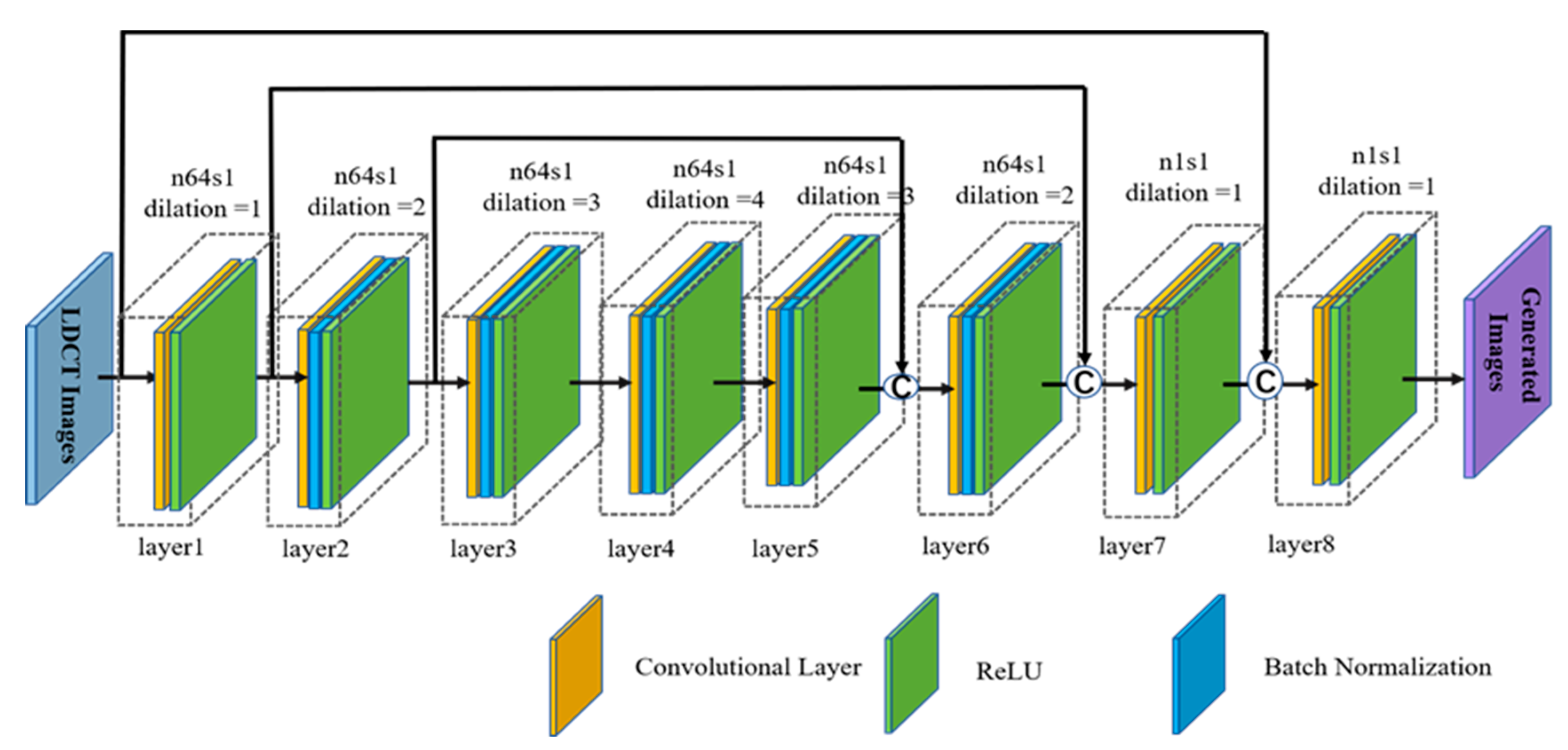
The generator is improved by the introduction of a convolutional neural network (CNN) with eight convolutional layers which is embedded in the residual structure and utilizes dilated convolutions. This improvement can increase the receptive field of the generator and fully mine the image information.
(2)
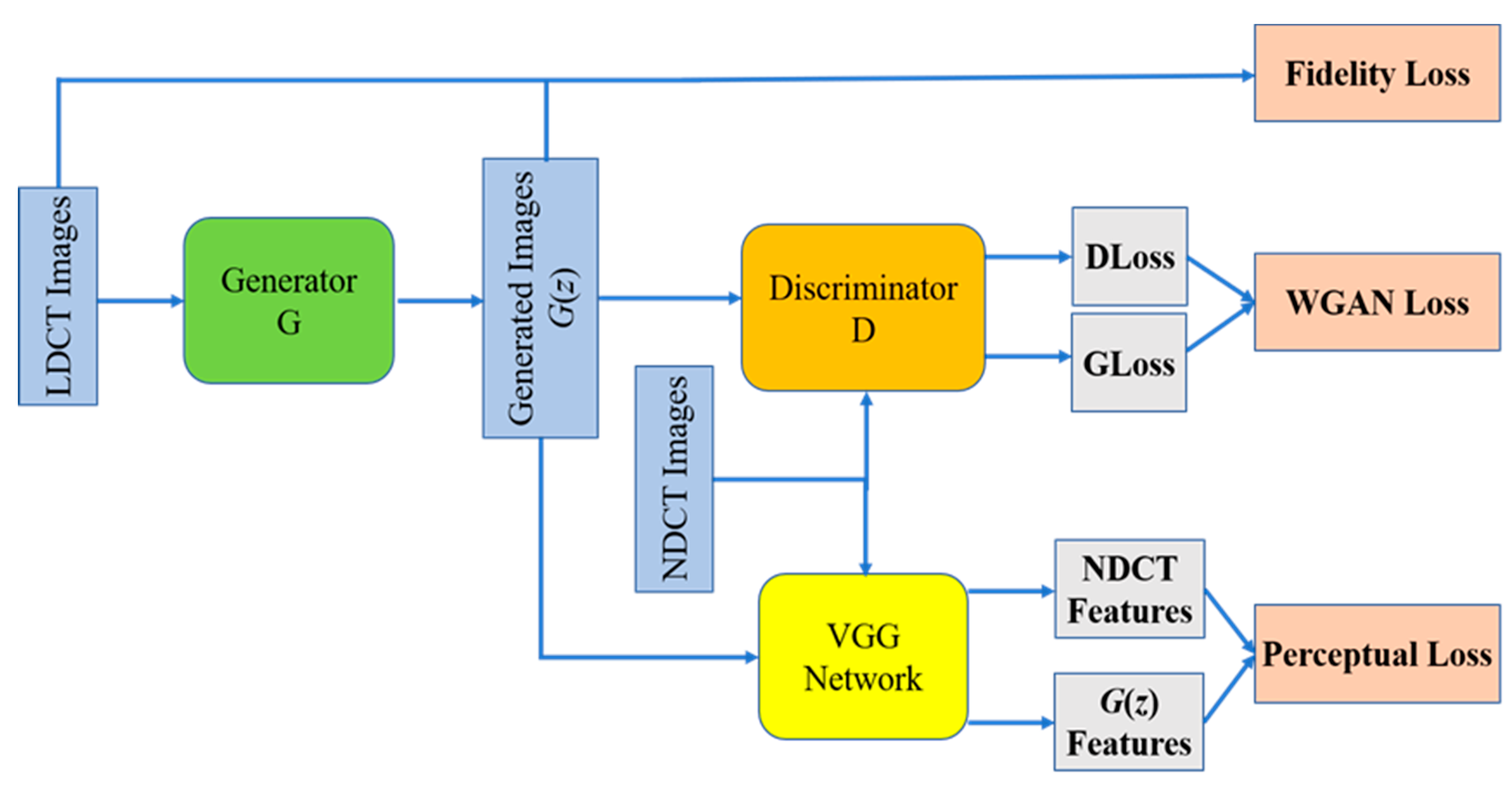
For the purpose of applying the feature space distribution of the unmatched clean images to guide the LDCT image denoising task, multi-perceptual loss is adopted to measure the difference between LDCT and NDCT images in feature space.
(3)
Since we use unpaired images for network training, we introduce a fidelity loss, which uses L2 loss to calculate the difference between the generated image and the original image to ensure that the generated image is not distorted.
The remainder of this paper is organized as follows. The proposed method based on WGAN with multi-perceptual loss and fidelity loss is introduced and presented in Section 2. Then, the experiments and analyses of the results are presented in Section 3. Lastly, Section 4 gives a summary of this paper and looks forward to some possible future research directions.

2. Methods

Suppose that z { z k } 1 N denotes the LDCT image, x { x k } 1 N denotes the unpaired NDCT image, and p l and p r represent the distribution of LDCT and NDCT images, respectively.

2.1. Wasserstein GAN

The denoising methods based on the traditional GAN [34,38] network use Jensen–Shannon (JS) divergence or Kullback–Leibler (KL) divergence to estimate the distance between two distributions. When the distance between the two distributions is far or there is no intersection at all, JS divergence will degenerate into a constant, and the KL divergence value will become meaningless; thus, they cannot be applied to the training task of unpaired CT images. In addition, the method based on GAN is prone to some problems such as gradient vanishing or explosion. To solve the above problems, a GAN model based on Wasserstein distance and 1-Lipschitz constraint is introduced. The model contains generator G and discriminator D. The training problem of G and D is expressed as follows:
min G max D L WGAN ( D , G )   =   E x ~ p r [ D ( x ) ]   +   E z ~ p l [ D ( G ( z ) ) ] + λ E x ^ ~ p x ^ [ ( | | x ^ D ( x ^ ) | | 2 1 ) 2 ] ,
where   G ( · ) , D ( · ) represent the outputs of G and D, respectively, E is the expectation of the dataset which conforms to a specific data distribution, and x ^ ~ p x ^ is obtained by random interpolation sampling on the line between the generated image and its corresponding NDCT image. The first two terms represent the Wasserstein distance between different data distributions, the third term is the gradient penalty factor used for regularization, and λ is the penalty coefficient.

2.2. Composition of Loss Functions

In order to use unpaired CT images to achieve the training of the denoising network and to achieve the performance of the denoising model based on paired images, two loss functions are designed in addition to the Wasserstein loss of WGAN itself.

2.2.1. Fidelity Loss

In the process of using unpaired CT image training generator G, due to the feature difference between the LDCT image and NDCT image, there will be a certain probability of structural loss in denoising results or there will be artefact. That is, there is the possibility of distortion for a generated image. Inspired by [32,39], fidelity loss is introduced to ensure the authenticity of denoising results. The function is expressed as follows:
L Fidelity = E z ~ p l [ 1 N 2 | | G ( z )     z | | 2 ] ,
where | | · | | 2 is L2-norm. Many scholars introduced L2-norm to measure the difference between the generated image and the corresponding NDCT image. A higher difference denotes higher quality of the generated image. However, as the method proposed is suitable for unpaired images (there is no correspondence between the LDCT image and NDCT image), instead of calculating the L2 loss between the generated image and the NDCT image, we calculate it between the generated image and the original image. In this way, the advantages of the L2-norm, which is a good constraint on the consistency of image pixels, are used to ensure the corresponding relationship between the generated image and the original image pixels.

2.2.2. Multi-Perceptual Loss

For medical image denoising, how to remove the noise while retaining more lesion features is one of the key research topics. People often use mean square error (MSE) as a loss function to measure the difference between denoised images and NDCT images. However, studies have found that a group of pictures with the same MSE value have significant differences in human subjective perception [40]. Moreover, it is meaningless to use MSE to measure the difference between the generated image and NDCT image for the image denoising task using unmatched images. Recent research proved that the use of trained CNN can obtain high-level image features [41,42], and the feature similarity between the generated image and the standard image can fully reflect the degree of semantic similarity between them. On the basis of this research, scholars proposed perceptual loss to guide image style conversion [43], image denoising [33], and other tasks.
Inspired by [33,43,44], the perceptual loss function is introduced to learn the feature distribution of NDCT images from the feature space to guide the denoising task of LDCT images. In this paper, we use a pre-trained network proposed by Visual Geometry Group (VGG) in Oxford named VGG-19 network (excluding the full connection layers of the last three layers) as the perceptual feature extractor, whereby five groups of feature maps are extracted in different levels and finally combined into multi-perceptual loss. Figure 1 shows the extraction methods of feature maps in different levels, which is expressed as follows:
L Perceptual = E ( x , z ) [ 1 w i h i d i i = 1 5 | | i ( G ( z ) )     i ( x ) | | 2 ] ,
where i is the feature map obtained from the block i, G (z) is the denoising result of the LDCT image, x represents the NDCT image, and w i , h i , and d i represent the width, height, and depth of the feature map, respectively. It should be noted that we use the VGG-19 network as the feature extractor. The input of the network is a color image, including three channels, while the CT image is a grayscale image. Therefore, before using the network for feature extraction, we duplicated the CT image to make RGB channels.

2.2.3. Full Objective

In order to improve the network’s denoising ability while retaining more content and texture information of CT images, a new composite loss function for unmatched CT image denoising is proposed as a function of WGAN loss, which combines fidelity loss and multi-perceptual loss. Our full objective is as follows:
L Multi - loss = λ 1 L WGAN + λ 2 L Fidelity + λ 3 L Perceptual ,
where λ 1 , λ 2 , and λ 3 are weighting parameters used to control the trade-off between the three loss functions.

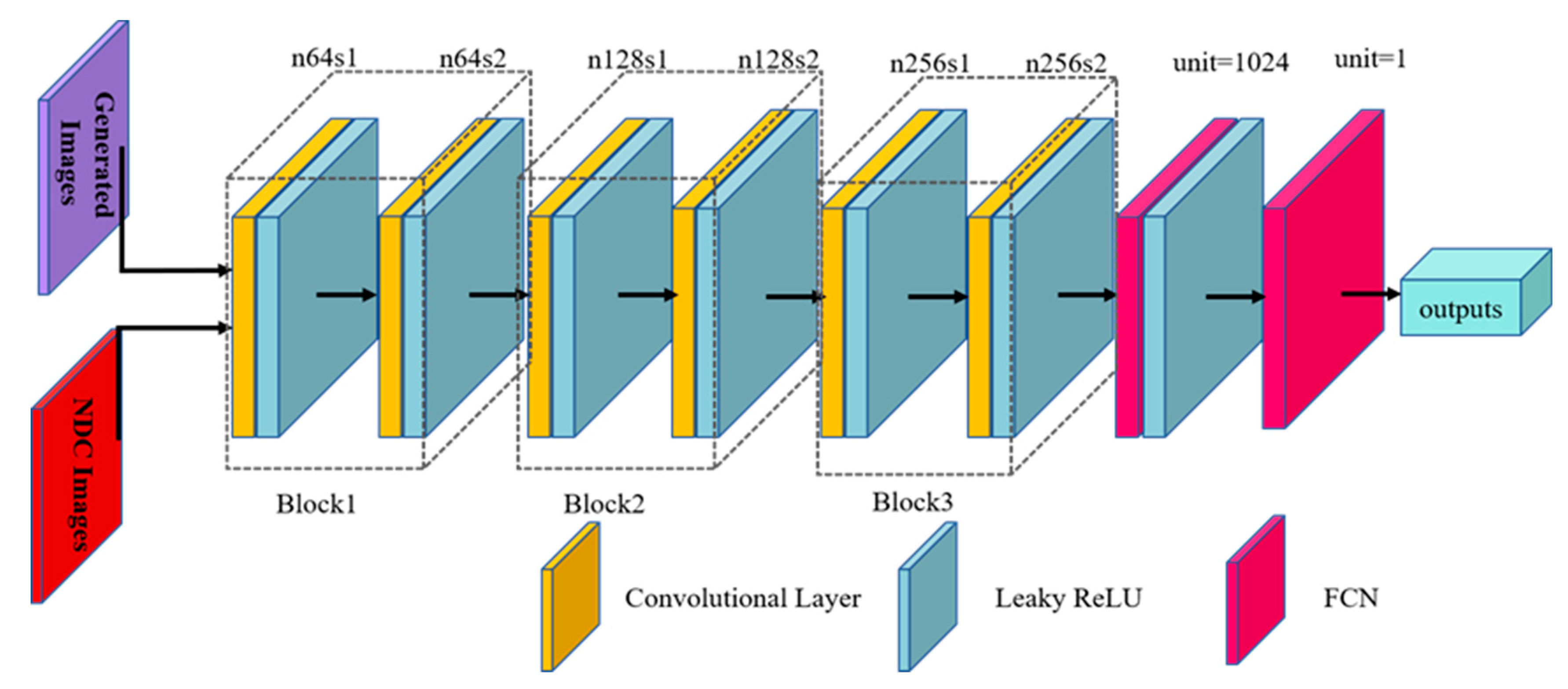
2.3. Network Structure

In order to better remove the noise in LDCT images, incorporating perceptual loss and fidelity loss, we propose a WGAN-based network, which uses a dilated convolution and residual structure. We named it as WGAN-based network, using dilated convolution and residual structure, with perceptual loss and fidelity loss. To simplify the description, we named the network DRWGAN-PF, in which D, R, WGAN, P, F stand for “dilated convolution”, “residual structure”, the structure of “Wasserstein GAN”, “perceptual loss” and “fidelity loss”, respectively.
The proposed network consists of three components. Figure 2 shows the overall network structure of the proposed method. First of all, a traditional convolution neural network is selected as the generator network. Substantial work has proven that, with the deepening of network layers, the network can obtain more image features, resulting in a better denoising effect. However, the increase in the number of network layers leads to the surge of training parameters and high dependence on the computing devices. In order to improve the network efficiency without increasing the complexity of the network, the residual structure, dilated convolution, and batch normalization are introduced. Figure 3 shows the structure of the generator network used in this paper.
We use a convolution neural network with eight convolution layers. The size of the convolution kernel in each convolution layer is 3   ×   3 . Rectified Linear Units, which is name as ReLU, is selected as the activation function. The number of filters in the first six convolution layers is set to 64, and the last two layers contain one. Batch normalization (BN) is added between the convolution layer and ReLU in the middle five convolution blocks. Studies have shown that a network with a larger perceptual field can get more context information, and dilated convolution can enhance the receptive field of network to a certain extent. Therefore, dilated convolution is applied in the second to sixth layers of the generator network, with dilated rates are 2, 3, 4, 3, and 2, respectively. Note that, when the expansion rate is 1, the dilated convolution degenerates into a traditional convolution layer. Lastly, to make full use of the detailed information of the input image, we use the idea of residual structure to connect the low-level image features with the high-level features of the image through skip connect, as shown in Figure 3.
The discriminator network adopts the network structure proposed in [33], as shown in Figure 4. The discriminator uses the traditional convolution neural network structure, the purpose of which is to distinguish whether the input image is a generated image or a real NDCT image. In short, it is a binary classification network in essence. The first six layers of the discriminator network are convolutional layers, which are divided into three blocks. The numbers of convolutional layer filters in Block1, Block2, and Block3 are set to 64, 128, and 256, respectively. LeakyReLU is selected as the activation function with a slope of 0.2. All the convolutional layers have a small 3 × 3 kernel size. The stride is set to be 1 for odd layers, and 2 for even layers. The last two layers are fully connected layers, and the outputs are 1024 and 1, respectively. Moreover, there is a LeakyReLU activation function after the first fully connected layer. As we adopt the WGAN framework, so there is no need to use the sigmoid cross-entropy layer at the end of the discriminator.
How to preserve more texture details while denoising low-dose CT images is an important issue. It is a very effective method to study image reconstruction and image denoising by using semantic features of images. Therefore, a feature extraction module, the VGG network shown in Figure 2, is added to the WGAN. The module uses the trained VGG-19 network as the feature extractor. The input is divided into two parts: one is the output G(z) of the generator, whereas the other is the unpaired NDCT image. It is found that the same type of images has certain similarity in semantic feature space. In this paper, a multi-perceptual extraction network is constructed on the basis of the VGG-19 network, as shown in Figure 1. In our method, the VGG-19 network with the last three layers of the full connection layer removed is divided into five blocks, and the output features of each block before MaxPooling are extracted to calculate the perceptual loss. Lastly, the difference in feature space between the generated image and the NDCT image is obtained using Equation (3).
Because there is no matching relationship between the NDCT image and the LDCT image used by us, the image generated by the generator is likely to be distorted if the model training is guided by WGAN loss and multi-perception loss. In response to this problem, we introduce a fidelity item, as shown in the “fidelity loss” module in Figure 1. The input of the module is the generated image and its corresponding LDCT image. The consistency of the generated image and the original image in terms of the overall structure and details is ensured by minimizing the difference between them.

3. Experiments and Results

3.1. Experimental Datasets

The data used in the experiment came from the LUNA16 dataset, and the image size was 512   ×   512 . We randomly selected 2500 CT images of 40 patients from this dataset, where 2400 images were selected for training, and the remaining 100 images were used for testing. We defined the selected 2500 CT images as NDCT images. Reference [45] pointed out that the noise distribution of LDCT images was approximately Gaussian; thus, so we obtained LDCT images by adding Gaussian noise to NDCT images.
The following protocol was used: we divided the NDCT image into two parts, selected the first part and its corresponding LDCT image for training the model on the basis of paired images, and selected the LDCT images of the first part and the NDCT images of the second part as the unpaired dataset for training the model proposed in this paper. In practice, the proposed method was executed in a patch-by-patch manner with a patch size of 128   ×   128 , in which images with mostly air were removed. Lastly, 11,648 pairs of image patches were used for training. It should be noted that the voxel values of CT images used in this paper varied from −3024 to 3071. Since the Hounsfield Unit (HU) value of the lung is about −500, the voxel values of each CT image were intercepted to [−1000, +400] and stored in a file of HDF5 after normalization.

3.2. Setting of the Parameters

In our work, all the experiments were carried out in the environment of TensorFlow on a computer with an Intel Core i7-9700K central processing unit (CPU), with 16 GB random-access memory (RAM) and NVIDIA RTX 2070s. It costs about 14 h to train our method. All networks were optimized using the Adam algorithm. Limited by the memory of the graphics processing unit (GPU), the size of each mini-batch was set to 32. The number of the epoch was set to 100. The hyperparameters of Adam were set as α   =   1   ×   10   4 , β 1   =   0 . 5 , and β 2   =   0 . 9 . Referring to [33], the value of λ in Equation (3) was set to 10. The values of λ 1 , λ 2 , and λ 3 in Equation (4) were set to 0.8, 0.1, and 0.1, respectively, according to our experimental experience.

3.3. Other Comparison Networks

In order to illustrate the performance of the network proposed in this paper, we trained another five networks, as shown in Table 1. “Dataset” in the table describes whether the data used in the network training is paired data or unpaired data. DRWGAN-PF is the method proposed in this paper. DRWGAN-F does not contain the perceptual loss function. GAN with fidelity loss (GAN-F) proposed in [32] is used for unpaired image denoising. WGAN with perceptual loss obtained by a pre-trained VGG-19 network (WGAN-VGG) proposed in [33], deep CNN denoiser prior for image restoration (IRCNN) proposed in [39] are used for paired image denoising. We also trained an IRCNN network with perceptual loss extracted by a pre-trained VGG-19 network (IRCNN-VGG) for image denoising. Moreover, λ 4 of GAN-F was set to 10, and the values of λ 5 , λ 6 in WGAN-VGG and IRCNN-VGG were equal to λ 3 .

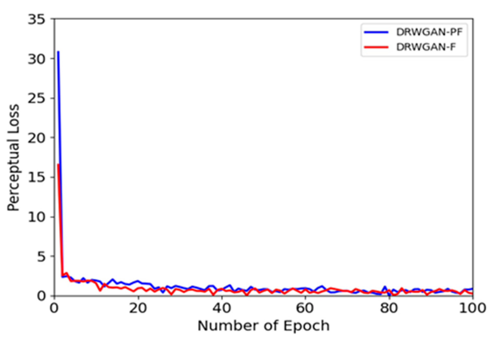
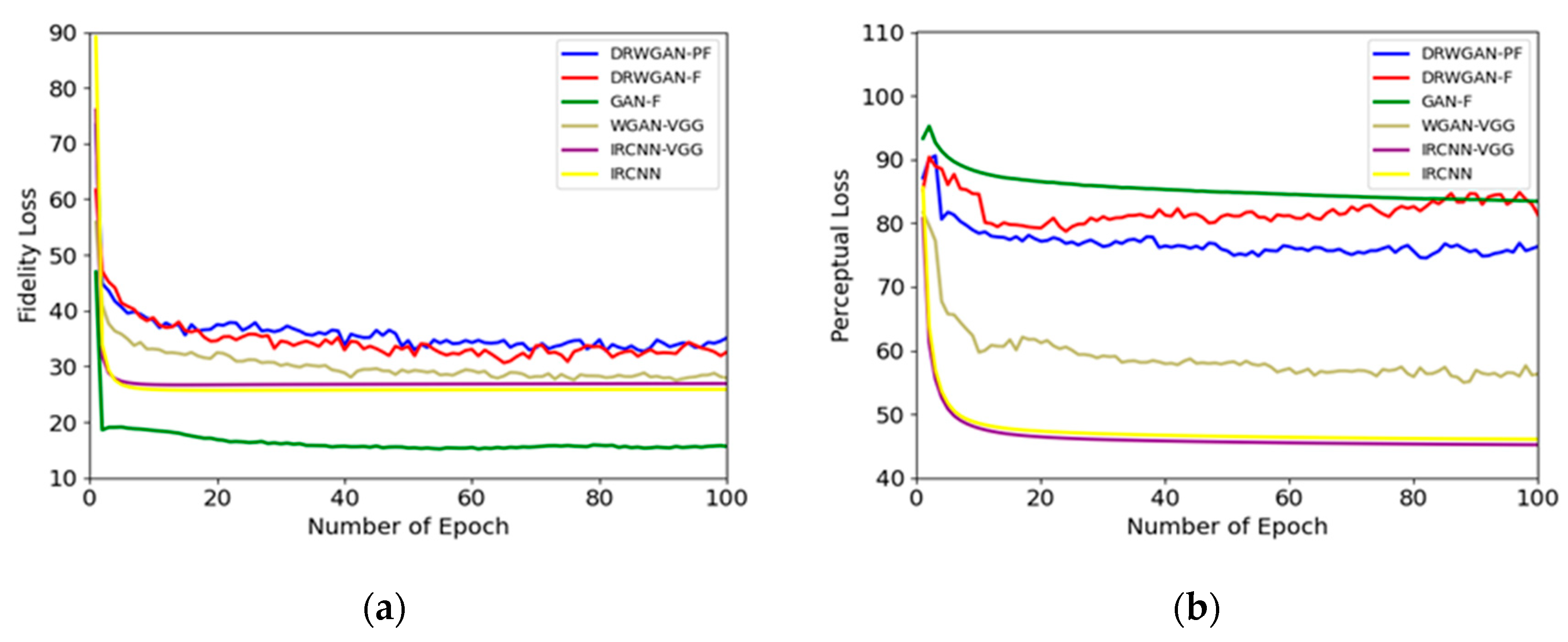
3.4. Network Convergence

Figure 5 displays the convergence during the training process of the network. It can be seen that, although the training process of the two networks was somewhat oscillatory, they eventually converged after the 20th epoch. Furthermore, we calculated the average value of each loss after each epoch during training. Figure 6 shows the change trend of each loss function with the number of iterations. Although some networks do not use the perceptual loss or fidelity loss function, this paper still presents the trend of the loss in the process of network training.
Figure 6a,b are the convergence of fidelity loss and perceptual loss, respectively. It can be seen that the two loss functions gradually decreased and eventually converged with the advancement of the training process. Figure 6a shows that the fidelity loss values of the three networks trained with unpaired data obeyed the following order: DRWGAN-PF > DRWGAN-F > GAN-F. It can be concluded from Equation (2) that fidelity loss measures the similarity between the denoising image and the LDCT image. A smaller value of fidelity loss denotes closer proximity of the generated image to the original LDCT image, which indicates that the distortion of the generated image is lower.
We can see that the changes in DRWGAN-PF and DRWGAN-F were more consistent; however, from a global point of view, the fidelity loss of the former was slightly higher than that of the latter. This is because the introduction of the multi-scale perceptual loss function made the generated image closer to the NDCT image in feature space. In other words, the NDCT image without noise could guide the generated image to remove the noise component in feature space. The elimination of noise components relatively increased the difference between the generated image and the original noise image. This phenomenon can also be seen in the three networks based on paired image training. For example, the fidelity loss of IRCNN-VGG with perceptual loss was slightly higher than that of IRCNN. The value of fidelity loss of GAN-F was much smaller because λ 4 in L Fidelity ( G ) of GAN-F was set to 10, accounting for a heavier proportion than the method proposed in this article, which resulted in the network paying more attention to the image distortion during the training process. Therefore, the image generated by GAN-F is closer to the original LDCT image, but it also retains more noise to a certain extent.
Perceptual loss measures the similarity between the generated image and the NDCT image in feature space. A smaller value denotes closer proximity of the generated image to the NDCT image in feature space. From Figure 6b, it can be seen that, compared to the DRWGAN-F, which does not minimize the perceptual loss, DRWGAN-PF, with minimizing the perceptual loss, could bring the generated image closer to the NDCT image in feature space. It should be pointed out that the perceptual loss of the network based on the unpaired image is generally high due to the significant difference in content between the generated image and the unpaired NDCT image. However, the change trend shows that the generated image is more and more similar to the clean image in high-level features, which also indicates the denoising effect of the network to a certain extent (because the features of the image with noise are more different from those of the NDCT image). It can also be seen from the figure that the proposed method has some advantages over the GAN-F method in image feature processing.

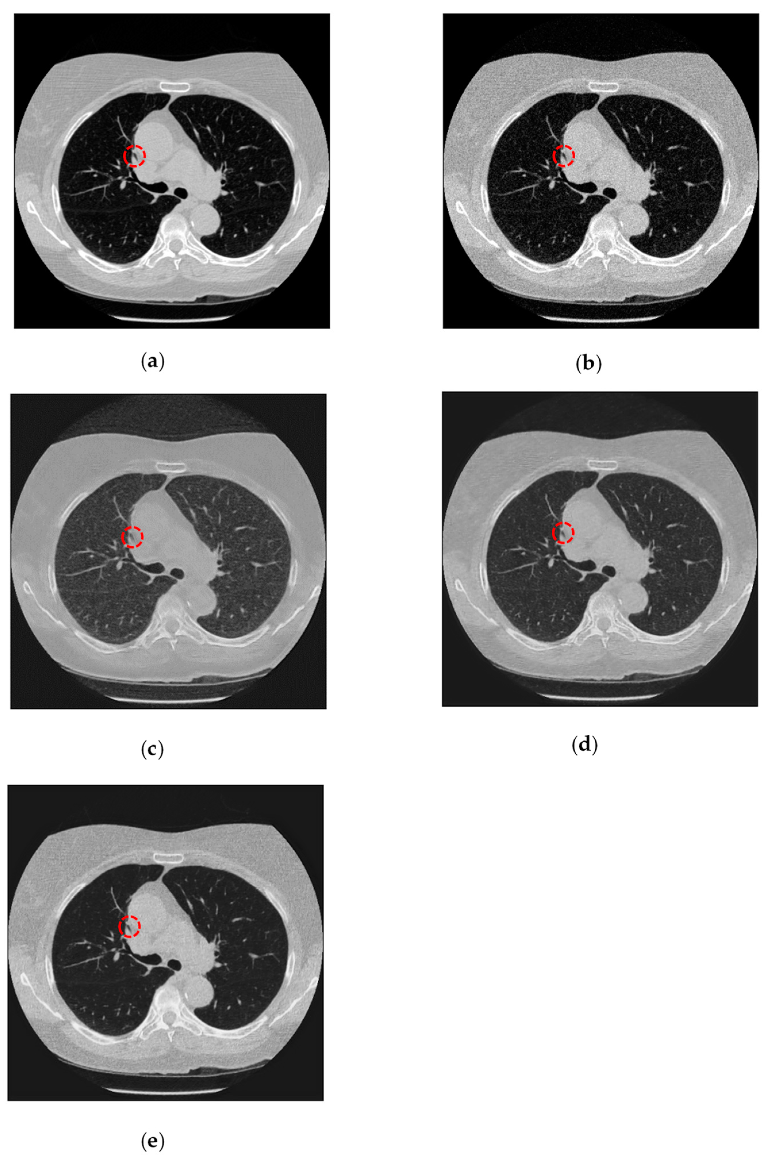
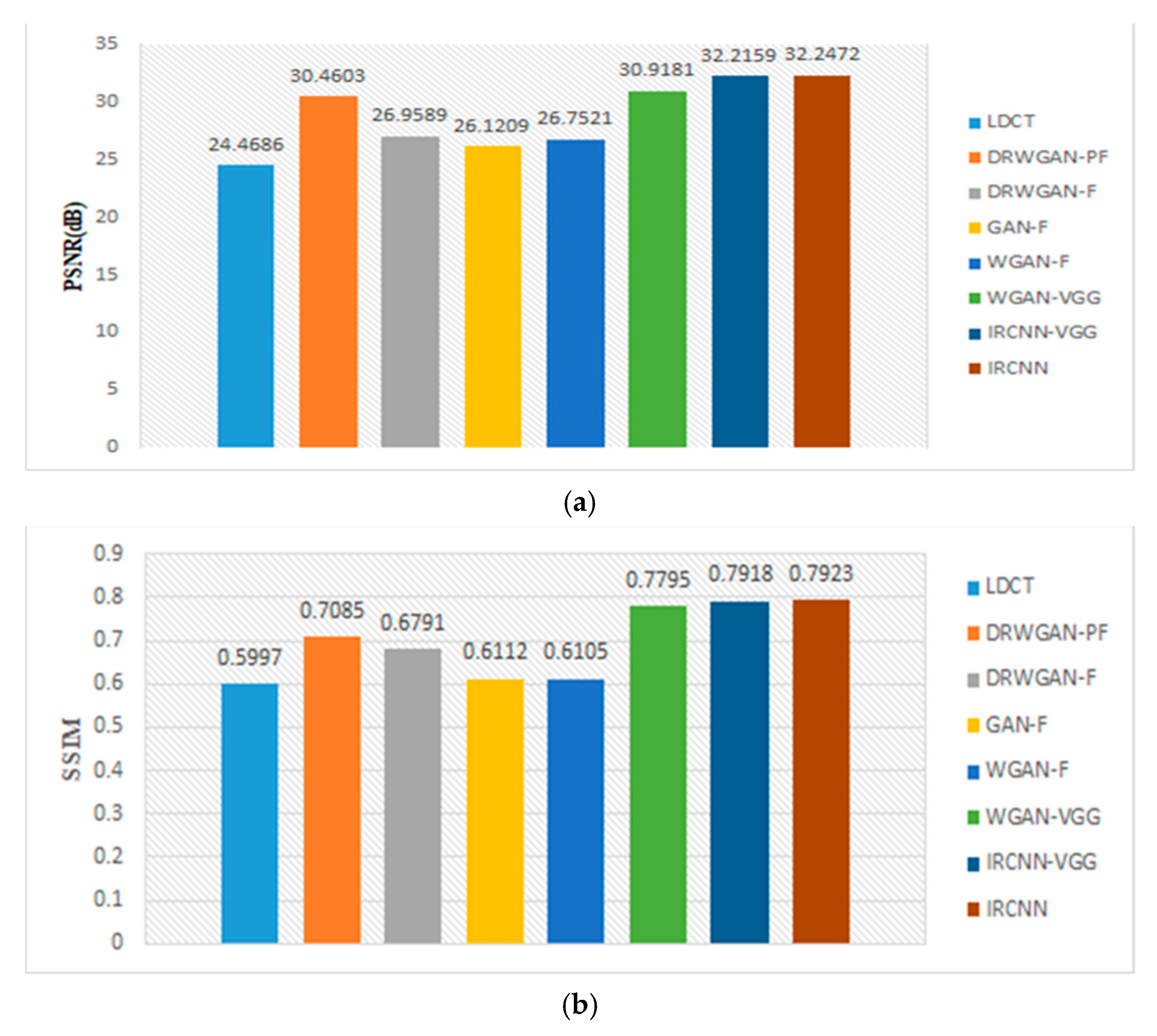
3.5. Results and Analysis

In order to demonstrate the denoising performance of the proposed DRWGAN-PF model based on the unpaired training set for LDCT images, we compare the denoising results of other methods in Table 1. Moreover, we used peak signal-to-noise ratio (PSNR) and structural similarity index measurement (SSIM) as the evaluation indices of image quality.
Using perceptual loss to improve image quality has been recognized by the majority of researchers; however, whether it is applicable to network training based on unpaired datasets remains to be verified. To this end, we implemented the DRWGAN-P network, which introduced multi-perceptual loss on the basis of DRWGAN. Figure 7 shows the generated images of DRWGAN, DRWGAN-P, and DRWGAN-PF. To quantitatively evaluate the performance of perceptual loss in networks trained on unpaired dataset, we calculated the PSNR and SSIM of the generated image, as shown in Table 2. From Table 2, we can find that, compared to DRWGAN, the PSNR and SSIM values of the image generated by DRWGAN-P were significantly improved, indicating that the perceptual loss can also be applied to the network trained based on unpaired datasets. This is because the perceptual loss measures the similarity of the two feature spaces, and the purpose is to use the semantic features of clean images to guide the denoising of LDCT images. Therefore, the perceptual loss could be used in the unpaired image denoising task.
Nevertheless, there are also some problems which occur during utilizing the perceptual loss. Combined with Figure 7, it can be seen that, compared to the hole marked in the red circle in Figure 7a,b, Figure 7d is smaller and fuzzy, while Figure 7e is closer to Figure 7a,b. This is because, when using the semantic features of clean images to guide LDCT denoising, the network learns the features that do not exist originally in LDCT images, thus resulting in distortion of the generated image. Therefore, we introduced a fidelity item while using the perceptual loss, aiming at ensuring that the generated image is not distorted while making use of the semantic features of the clean image.
For the sake of intuitively showing the denoising effect of DRWGAN-PF, we selected a representative CT slice for qualitative comparison (see Figure 8). It can be seen from Figure 8 that the two methods based on paired training data and unpaired training data achieved good denoising results.
Figure 8c,d,g are denoising images based on matched training data. It can be found that Figure 8c is more delicate and smoother, but slightly inferior to Figure 8d,g in terms of visual effect. The reason for this phenomenon is that IRCNN uses MSE as the loss function, and MSE measures the difference between the generated image and NDCT image pixel by pixel; thus, the image generated via this method is smoother. However, IRCNN-VGG and WGAN-VGG networks with perceptual loss can partly retain the perceptual features of an image, which brings the generated images closer to NDCT images in terms of visual perception. Although Figure 8f has less noise than Figure 8e, Figure 8e is closer to the lung parenchyma part of NDCT image. The difference between GAN-F and WGAN-F is that the former uses the U-Net network with a shortcut as the generator, and the latter uses the eight-layer CNN network as the generator, which indicates that the performance of the generator based on the traditional CNN network needs to be improved. Comparing the yellow rectangular areas in Figure 8f,h, it is not difficult to find that the DRWGAN network with the introduction of the dilated convolution and the residual structure has significantly improved image denoising and detail preservation.
The enlarged view of the red rectangular area in Figure 8 is shown in Figure 9. Due to the interference of noise, the details in the red circular area in Figure 9b become more blurred. Comparing the generated images, it can be seen that the quality of various low-dose denoising algorithms has been significantly improved compared with the original LDCT image. It is not difficult to observe that Figure 9c is too smooth compared to Figure 9d, and Figure 9d is closer to the NDCT image in terms of visual features, which supports the effectiveness of the perceptual loss mentioned above. Through comparison, it can be found that the image quality obtained using the method in Figure 9e is relatively low, because the fidelity loss results in GAN-F paying more attention to the similarity between the generated image and the LDCT image during the training process, resulting in the generated image retaining much more noise, which can also be seen in Figure 9h. By comparing Figure 9h,i, we can see that the quality of the image changes significantly after the introduction of multi-perceptual loss. Moreover, the introduction of multi-perceptual loss also makes the generated image retain more detail.
For the purpose of quantitatively analyzing the denoising ability of each network, we calculated the average values of PSNR and SSIM of the generated images (generated from the 100 LDCT images in the test dataset), as shown in Figure 10. From Figure 10, we can see that the objective index of the IRCNN method based on MSE loss is the highest, but it is not difficult to see that this method does not show advantages in a subjective evaluation by comparing with the images in Figure 8. Compared with the three methods based on pairing image training, the objective evaluation index of the proposed method is very close to that of the network based on paired data and is higher than the method proposed in [32]. Moreover, by comparing WGAN-PF and WGAN-F, we once again confirmed that it is feasible to obtain the feature similarity between the generated image and the NDCT image from the feature space through multi-perceptual loss to guide the denoising task of network based on unpaired images.

4. Conclusions

How to train denoising models with unpaired data is an important topic in the field of medical image processing. In our work, we propose an adversarial denoising network that integrates fidelity terms and multi-perceptual loss for LDCT image denoising. The network proposed in this paper does not require matching of LDCT and NDCT images. The multi-perceptual loss optimizes the quality of the generated image by minimizing the feature space similarity between the generated image and the unpaired NDCT image, but this will cause image distortion to a certain extent. Aiming at this problem, a data fidelity function is proposed to ensure that there are no artificial features in the generated image by minimizing the L2 loss of the generated image and the original noise image. Through the training, the balance point of the two minimization processes can always be found, so that the generated image quality is closer to the NDCT image without losing or adding artificial features. In addition, the introduction of residual structure and dilated convolution also enhances the image generation capabilities of traditional CNN networks.
The experimental results show that the proposed network has an acceptable noise suppression effect while maintaining the texture and edge information of low-dose CT images. The subjective analysis and objective evaluation index scores are used to evaluate the image quality, which also prove that the proposed denoising method can significantly improve the image quality.

Author Contributions

Conceptualization, Z.Y.; data curation, Z.Y. and Z.H.; formal analysis, Z.Y. and K.X.; funding acquisition, Z.Y., K.X., and B.Z.; investigation, Z.Y., J.Z., and S.W.; methodology, Z.Y.; project administration, Z.Y. and K.X.; software, Z.Y.; supervision, K.X.; training, Z.Y. and Z.H.; validation, Z.Y. and J.Z.; visualization, Z.Y. and S.W.; original draft writing, Z.Y.; review and editing, Z.Y. and K.X. All authors have read and agreed to the published version of the manuscript.

Funding

This research was funded by the “Key Supporting Project of the Joint Fund of the National Natural Science Foundation of China, No. U1813222”, the “Tianjin Natural Science Foundation, No.18JCYBJC16500”, the “Key Research and Development Project from Hebei Province, No.19210404D”, and “The Other Commissions Project of Beijing No. Q6025001202001”.

Institutional Review Board Statement

Not applicable.

Informed Consent Statement

Not applicable.

Data Availability Statement

Publicly available datasets were analyzed in this study. This data can be found here: [https://luna16.grand-challenge.org/Data/].

Conflicts of Interest

The authors declare no conflict of interest.

References

  1. de Gonzalez, A.B.; Darby, S. Risk of cancer from diagnostic X-rays: Estimates for the UK and 14 other countries. Lancet 2004, 363, 345–351. [Google Scholar] [CrossRef]
  2. Bindman, S.; Rebecca, C.T. Radiation and the Risk of Cancer. Curr. Radiol. Rep. 2015, 3, 1–7. [Google Scholar]
  3. Naidich, D.P.; Marshall, C.H.; Gribbin, C.; Arams, R.S.; McCauley, D.I. Low-dose CT of the lungs: Preliminary observations. Radiology 1990, 175, 729–731. [Google Scholar] [CrossRef] [PubMed]
  4. Mori, I.; Machida, Y.; Osanai, M.; Linuma, K. Photon starvation artifacts of X-ray CT: Their true cause and a solution. Radiol. Phys. Technol. 2013, 6, 130–141. [Google Scholar] [CrossRef] [PubMed]
  5. Whiting, B.R. Signal statistics in x-ray computed tomography. Proc. SPIE Int. Soc. Opt. Eng. 2002, 4682, 53–60. [Google Scholar]
  6. Wang, J.; Li, T.; Lu, H.; Liang, Z. Penalized weighted least-squares approach to sinogram noise reduction and image reconstruction for low-dose X-ray computed tomography. IEEE Trans. Med. Imaging 2006, 25, 1272–1283. [Google Scholar] [CrossRef]
  7. Hsieh, J. Adaptive streak artifact reduction in computed tomography resulting from excessive x-ray photon noise. Med. Phys. 1998, 25, 2139–2147. [Google Scholar] [CrossRef]
  8. Demirkaya, O. Reduction of noise and image artifacts in computed tomography by nonlinear filtration of projection images. Proc. SPIE 2001, 4322. [Google Scholar]
  9. Yu, L.; Manduca, A.; Trzasko, J.D.; Khaylova, N.; Kofler, J.M.; McCollough, C.M.; Fletcher, J.G. Sinogram smoothing with bilateral filtering for low-dose CT. Proc. SPIE Int. Soc. Opt. Eng. 2008, 6913, 691329. [Google Scholar]
  10. Cui, X.; Zhang, Q.; Shangguan, H.; Liu, Y.; Gui, Z. The adaptive sinogram restoration algorithm based on anisotropic diffusion by energy minimization for low-dose X-ray CT. Optik-Int. J. Light Electron Opt. 2014, 125, 1694–1697. [Google Scholar] [CrossRef]
  11. Smith, P.R.; Peters, T.M.; Bates, R.H.T. Image reconstruction from finite numbers of projections. J. Phys. A Math. Nucl. Gen. 2001, 6, 319–381. [Google Scholar] [CrossRef]
  12. Manduca, A.; Yu, L.F.; Trzasko, J.D.; Khaylova, N. Projection space denoising with bilateral filtering and CT noise modeling for dose reduction in CT. Med. Phys. 2009, 36, 4911–4919. [Google Scholar] [CrossRef] [PubMed]
  13. Beister, M.; Kolditz, D.; Kalender, W.A. Iterative reconstruction methods in X-ray CT. Phys. Med. 2012, 28, 94–108. [Google Scholar] [CrossRef] [PubMed]
  14. Sidky, E.Y.; Pan, X. Image reconstruction in circular cone-beam computed tomography by constrained, total-variation minimization. Phys. Med. Biol. 2008, 53, 4777–4807. [Google Scholar] [CrossRef] [Green Version]
  15. Chen, Y.; Gao, D.; Nie, C.; Luo, L.; Chen, W.; Yin, X.; Lin, Y. Bayesian statistical reconstruction for low-dose X-ray computed tomography using an adaptive-weighting nonlocal prior. Comput. Med. Imaging Graph. 2009, 33, 495–500. [Google Scholar] [CrossRef]
  16. Zhang, Q.; Gui, Z.; Chen, Y.; Li, Y.; Luo, L. Bayesian sinogram smoothing with an anisotropic diffusion weighted prior for low-dose X-ray computed tomography. Opt. Int. J. Light Electron. Opt. 2013, 124, 2811–2816. [Google Scholar] [CrossRef]
  17. Tang, S.; Wang, R.; Wei, Y.; Ming, J.; He, Z. Research of Tongue Image Denoising Based on Partial Differential Equation. Comput. Eng. 2012, 38, 190–192. [Google Scholar]
  18. Zhang, Y.; Wang, Y.; Zhang, W.; Lin, F.; Pu, Y.; Zhou, J. Statistical iterative reconstruction using adaptive fractional order regularization. Biomed. Opt. Express 2016, 7, 1015–1029. [Google Scholar] [CrossRef] [Green Version]
  19. Chen, B.; Zhang, C.; Bian, Z.; Chen, W.; Ma, J.; Zhou, Q.; Zhou, X. Sparse-View X-ray Computed Tomography Reconstruction via Mumford-Shah Total Variation Regularization. Int. Conf. Intell. Comput. 2015, 9227, 745–751. [Google Scholar]
  20. Alenius, S.; Ruotsalaine, U. Attenuation correction for PET using count-limited transmission images reconstructed with median root prior. IEEE Trans. Nucl. Sci. 1999, 46, 646–651. [Google Scholar] [CrossRef]
  21. Zhan, H.; Ma, J.; Wang, J.; Moore, W.; Liang, Z. Assessment of prior image induced nonlocal means regularization for low-dose CT reconstruction: Change in anatomy. Med. Phys. 2017, 44, e264–e278. [Google Scholar] [CrossRef] [PubMed] [Green Version]
  22. Cheng, L.; Zhang, Y.; Song, Y.; Li, C.; Guo, D. Low-Dose CT Image Restoration Based on Adaptive Prior Feature Matching and Nonlocal Means. Int. J. Image Graph. 2019, 19, 1950017. [Google Scholar] [CrossRef]
  23. Niu, S.; Zhang, S.; Huang, J.; Bian, Z.; Chen, W.; Yu, G.; Liang, Z.; Ma, J. Low-dose cerebral perfusion computed tomography image restoration via low-rank and total variation regularizations. Neurocomputing 2016, 197, 143–160. [Google Scholar] [CrossRef] [Green Version]
  24. Chen, W.; Shao, Y.; Jia, L.; Wang, Y.; Gui, Z. Low-Dose CT Image Denoising Model Based on Sparse Representation by Stationarily Classified Sub-Dictionaries. IEEE Access 2019, 7, 116859–116874. [Google Scholar] [CrossRef]
  25. Hasan, A.M.; Melli, A.; Wahid, K.A.; Babyn, P. Denoising Low-Dose CT Images Using Multiframe Blind Source Separation and Block Matching Filter. IEEE Trans. Radiat. Plasma Med. Sci. 2018, 2, 279–287. [Google Scholar] [CrossRef]
  26. Lecun, Y.; Bengio, Y.; Hinton, G. Deep learning. Nature 2015, 521, 436–444. [Google Scholar] [CrossRef]
  27. Chen, H.; Zhang, Y.; Zhang, W.; Liao, P.; Wang, G. Low-dose CT denoising with convolutional neural network. In Proceedings of the 2017 IEEE 14th International Symposium on Biomedical Imaging, Melbourne, Sydney, 18–21 April 2017; pp. 143–146. [Google Scholar]
  28. Chen, H.; Zhang, Y.; Mannudeep, K.; Lin, F.; Chen, Y.; Liao, P.; Zhou, J.; Wang, G. Low-Dose CT with a Residual Encoder-Decoder Convolutional Neural Network. IEEE Trans. Med. Imaging 2017, 36, 2524–2535. [Google Scholar] [CrossRef]
  29. Kang, E.; Min, J.; Ye, J. A deep convolutional neural network using directional wavelets for low‐dose X‐ray CT reconstruction. Med. Phys. 2017, 44, e360–e375. [Google Scholar] [CrossRef] [Green Version]
  30. Kang, E.; Min, J.; Ye, J. Wavelet Domain Residual Network (WavResNet) for Low-Dose X-ray CT Reconstruction. arXiv 2017, arXiv:1703.01383. [Google Scholar]
  31. Ye, J.; Han, Y.; Cha, E. Deep convolutional framelets: A general deep learning framework for inverse problems. SIAM J. Imaging Sci. 2018, 11, 991–1048. [Google Scholar] [CrossRef]
  32. Park, H.S.; Baek, J.; You, S.K.; Choi, J.K.; Seo, J.K. Unpaired image denoising using a generative adversarial network in X-ray CT. IEEE Access 2019, 7, 110414–110425. [Google Scholar] [CrossRef]
  33. Yang, Q.; Yan, P.; Zhang, Y.; Yu, H.; Shi, Y.; Mou, X.; Kalra, M.K.; Zhang, Y.; Sun, L.; Wang, G. Low-Dose CT Image Denoising Using a Generative Adversarial Network with Wasserstein Distance and Perceptual Loss. IEEE Trans. Med. Imaging 2018, 37, 1348–1357. [Google Scholar] [CrossRef] [PubMed]
  34. Tang, C.; Li, J.; Wang, L.; Li, Z.; Yan, B. Unpaired Low-Dose CT Denoising Network Based on Cycle-Consistent Generative Adversarial Network with Prior Image Information. Comput. Math. Methods Med. 2019, 2019, 1–11. [Google Scholar] [CrossRef] [PubMed]
  35. Arjovsky, M.; Chintala, S.; Bottou, L. Wasserstein GAN. arXiv 2017, arXiv:1701.07875. [Google Scholar]
  36. Champion, T.; Pascale, L.D.; Juutinen, P. The ∞-Wasserstein Distance: Local Solutions and Existence of Optimal Transport Maps. SIAM J. Math. Anal. 2008, 40, 1–20. [Google Scholar] [CrossRef]
  37. Gulrajani, I.; Ahmed, F.; Arjovsky, M.; Dumoulin, V.; Courville, A. Improved Training of Wasserstein GANs. arXiv 2017, arXiv:1704.00028. [Google Scholar]
  38. Goodfellow, I.; Pouget-Abadie, J.; Mirza, M.; Xu, B.; Warde-Farley, D.; Ozair, S.; Courville, A.; Bengio, Y. Generative Adversarial Nets. Adv. Neural Inf. Process. Syst. 2014, 3, 2672–2680. [Google Scholar]
  39. Zhang, K.; Zuo, W.; Gu, S.; Zhang, L. Learning Deep CNN Denoiser Prior for Image Restoration. In Proceedings of the 2017 IEEE Conference on Computer Vision and Pattern Recognition, Honolulu, HI, USA, 21 July 2017; pp. 2808–2817. [Google Scholar]
  40. Wang, Z.; Bovik, A.C.; Sheikh, H.R.; Simoncelli, E.P. Image quality assessment: From error visibility to structural similarity. IEEE Trans. Image Process 2004, 13, 600–612. [Google Scholar] [CrossRef] [Green Version]
  41. Mahendran, A.; Vedaldi, A. Understanding deep image representations by inverting them. In Proceedings of the 2015 IEEE Conference on Computer Vision and Pattern Recognition, Boston, MA, USA, 7–12 June 2015; pp. 5188–5196. [Google Scholar]
  42. Simonyan, K.; Vedaldi, A.; Zisserman, A. Deep Inside Convolutional Networks: Visualising Image Classification Models and Saliency Maps. arXiv 2013, arXiv:1312.6034. [Google Scholar]
  43. Johnson, J.; Alahi, A.; Li, F. Perceptual Losses for Real-Time Style Transfer and Super-Resolution. In Proceedings of the European Conference on Computer Vision, Amsterdam, The Netherlands, 11–14 October 2016. [Google Scholar]
  44. Gholizadeh-Ansari, M.; Alirezaie, J.; Babyn, P. Deep Learning for Low-Dose CT Denoising. arXiv 2019, arXiv:1902.10127. [Google Scholar]
  45. Lu, H.; Hsiao, I.T.; Li, X.; Liang, Z. Noise properties of low-dose CT projections and noise treatment by scale transformations. Nucl. Sci. Symp. Conf. Rec. 2001, 3, 1662–1666. [Google Scholar]
Figure 1. Multi-perceptual loss network architecture.
Symmetry 13 00126 g001
Figure 2. Schematic overview of the DRWGAN-PF model.
Symmetry 13 00126 g002
Figure 3. The structure of the generator network, where n stands for the number of convolutional kernels, s stands for convolutional stride, and dilation stands for convolution operator with dilatation rate i (i = 1, 2, 3, 4); © stands for the concatenation operation.
Symmetry 13 00126 g003
Figure 4. The structure of the discriminator network, where n and s have the same meaning as in Figure 3.
Symmetry 13 00126 g004
Figure 5. Wasserstein Distance curves of DRWGAN-PF and DRWGAN-F.
Symmetry 13 00126 g005
Figure 6. Comparison of loss function value versus the number of epochs with respect to different algorithms: (a) fidelity loss; (b) perceptual loss.
Symmetry 13 00126 g006
Figure 7. Denoising results of DRWGAN-P and DRWGAN-PF trained on unpaired dataset: (a) normal-dose computed tomography (NDCT) image; (b) low-dose computed tomography (LDCT) image with Gaussian noise; (c) DRWGAN; (d) DRWGAN-P; (e) DRWGAN-PF.
Symmetry 13 00126 g007
Figure 8. Denoising results of the different algorithms on lung dataset in lung window: (a) NDCT image; (b) LDCT image with Gaussian noise; (c) IRCNN; (d) IRCNN-VGG; (e) GAN-F; (f) WGAN-F; (g) WGAN-VGG; (h) DRWGAN-F; (i) DRWGAN-PF.
Symmetry 13 00126 g008
Figure 9. Zoomed region of interest (ROI) of the red rectangle in Figure 8: (a) NDCT image; (b) LDCT image with Gaussian noise; (c) IRCNN; (d) IRCNN-VGG; (e) GAN-F; (f) WGAN-F; (g) WGAN-VGG; (h) DRWGAN-F; (i) DRWGAN-PF.
Symmetry 13 00126 g009
Figure 10. The mean PSNR and SSIM of the images in test dataset generated by the different algorithms: (a) PSNR; (b) SSIM.
Symmetry 13 00126 g010
Table 1. Details of all networks trained in this paper.
NetworkLossDataset
DRWGAN-PF min G max D λ 1 L WGAN ( G ,   D ) + λ 2 L Fidelity ( G ) + λ 3 L Perceptual ( G ) Unpaired
DRWGAN-F min G max D λ 1 L WGAN ( G ,   D ) + λ 2 L Fidelity ( G ) Unpaired
GAN-F min G max D L GAN ( G ,   D ) + λ 4 L Fidelity ( G ) Unpaired
WGAN-VGG min G max D L WGAN ( G ,   D ) + λ 5 L VGG ( G ) Paired
IRCNN min G L MSE ( G ) Paired
IRCNN-VGG min G L MSE ( G ) + λ 6 L Perceptual ( G ) Paired
Table 2. Performance of DRWGAN-P and DRWGAN-PF using unpaired dataset. PSNR, peak signal-to-noise ratio; SSIM, structural similarity.
MetricLDCTDRWGANDRWGAN-PDRWGAN-PF
PSNR24.524123.488529.209129.6957
SSIM0.54540.59470.62330.6916
Publisher’s Note: MDPI stays neutral with regard to jurisdictional claims in published maps and institutional affiliations.

