Elite Exploitation: A Combination of Mathematical Concept and EMO Approach for Multi-Objective Decision Making


School of Computer Science and Technology, Qilu University of Technology (Shandong Academy of Sciences), Jinan 250353, China
*
Author to whom correspondence should be addressed.
Symmetry 2021, 13(1), 136; https://0-doi-org.brum.beds.ac.uk/10.3390/sym13010136
Submission received: 30 December 2020
/
Revised: 7 January 2021
/
Accepted: 11 January 2021
/
Published: 15 January 2021
(This article belongs to the Section Computer)
Abstract
:This paper explores the combination of a classic mathematical function named “hyperbolic tangent” with a metaheuristic algorithm, and proposes a novel hybrid genetic algorithm called NSGA-II-BnF for multi-objective decision making. Recently, many metaheuristic evolutionary algorithms have been proposed for tackling multi-objective optimization problems (MOPs). These algorithms demonstrate excellent capabilities and offer available solutions to decision makers. However, their convergence performance may be challenged by some MOPs with elaborate Pareto fronts such as CFs, WFGs, and UFs, primarily due to the neglect of diversity. We solve this problem by proposing an algorithm with elite exploitation strategy, which contains two parts: first, we design a biased elite allocation strategy, which allocates computation resources appropriately to elites of the population by crowding distance-based roulette. Second, we propose a self-guided fast individual exploitation approach, which guides elites to generate neighbors by a symmetry exploitation operator, which is based on mathematical hyperbolic tangent function. Furthermore, we designed a mechanism to emphasize the algorithm’s applicability, which allows decision makers to adjust the exploitation intensity with their preferences. We compare our proposed NSGA-II-BnF with four other improved versions of NSGA-II (NSGA-IIconflict, rNSGA-II, RPDNSGA-II, and NSGA-II-SDR) and four competitive and widely-used algorithms (MOEA/D-DE, dMOPSO, SPEA-II, and SMPSO) on 36 test problems (DTLZ1–DTLZ7, WGF1–WFG9, UF1–UF10, and CF1–CF10), and measured using two widely used indicators—inverted generational distance (IGD) and hypervolume (HV). Experiment results demonstrate that NSGA-II-BnF exhibits superior performance to most of the algorithms on all test problems.
1. Introduction
Compared to those with a single objective, multi-objective optimization problems (MOPs) [1] always have greater complexity. Let us assume there is an engineer who wants to build an ideal building: inexpensive, high-rise, novel architectural image, earthquake-resistant, and energy-efficient. Isn’t that a great idea? Unfortunately, such a building cannot be built as these goals cannot be met simultaneously. Thus, in real-world engineering, we have a concept called multi-objective optimization problems (MOPs) with several objectives that are conflicted with each other and can be modeled by
where is a decision vector within the search space , n is the dimensions of the decision vector, and m is the number of objective functions to be optimized. A set of solutions generally solves them called Pareto optimal set (PS). The map of a PS in the objective space is called a Pareto front (PF), and the goal of algorithms that aim to solve MOPs is to search a set of approximate solutions for the map that is the closest to the true PF, meanwhile, with good diversity.
Recently, heuristic algorithms have been regarded as the primary method for solving MOPs. These algorithms can be classified into three categories [2]: Pareto-based multi-objective evolutionary algorithms (MOEAs) [3,4,5,6,7,8,9,10,11,12], indicator-based MOEAs [13,14,15,16,17,18,19], and decomposi tion-based MOEAs [20,21,22,23,24,25,26,27,28,29,30].
Dominance-based MOEAs use the concept of dominance relation into the selection of the evolutionary process, some wildly used algorithms such as SPEA2 [4], NSGA-II [5], and some variations like NSGA-II-SDR [6], an adaptive niching technique based on the angles between the candidate solutions is proposed. Meanwhile, some particle swarm optimizations (PSO) like SMOPSO [9] are characterized by the use of a strategy to limit the velocity of the particles. XPSO [7] transplants the multi-exemplar and forgetting ability to particle swarm optimization, and TSLPSO [8] proposes a dimensional learning strategy for discovering and integrating the promising information to improve the search efficiency.
Indicator-based MOEAs use different indicators to estimate their density and guide the evolutionary process. Recently, an IGD indicator-based algorithm has been proposed in Reference [18]. In Reference [19], an indicator called I-SDE(+), which combines the sum of objectives and shift-based density, is proposed. What is more, in rNSGA-II [15], a variation of Pareto dominance was proposed, which creates a strict partial order among Pareto solutions and enables decision-makers to guide the search using a set of aspiration levels.
Decomposition-based MOEAs transform MOPs into a series of single-objective optimization subproblems and optimize them collaboratively. MOEA/D [27] is a famous and widely used MOEA based on the decomposition framework, with variations like MOEA/D-DE [23], which has a differential evolution operator and a polynomial mutation operator. In some followed up works like dMOPSO [30] a memory reinitialization process is used to provide diversity. In NSGA-IIconflict [29], they separate MOPs into several subproblems, and use the conflict information to partition the objective space. Furthermore, in RPDNSGA-II [24], they defined a decomposition-based dominance relation and a novel diversity factor to create a strict partial order in a solution set. For more details of recent MOEAs, please refer to References [31,32].
All these works obtained cheerful achievement in the past decades. However, the global exploration’s outstanding performance also causes the neglect of individual exploitation, leading to insufficient diversity and a lack of convergence performance in the PS when facing MOP with complex PF. Thus, the hybrid algorithm frameworks [33,34] have been proposed. These algorithms generally contain an individual exploitation operator, which is usually performed by an existing search operator from another algorithm (i.e., a search operator of an existing algorithm is nested inside another algorithm). However, we do not recommend this structure because it may lead to the overconsumption of computational resources. We can also learn from paper [35] that there are at least two basic requirements for a competitive hybrid algorithm framework: (1) a resource allocation strategy and (2) a simple and effective individual exploitation operator. Inspired by this conclusion, we propose a hybrid genetic algorithm.
In this paper, we propose a variation of NSGA-II called NSGA-II-BnF with an elite exploitation strategy, which mainly contains the following two parts: first, for maintaining diversity, a biased resource allocation strategy is proposed, which selects elites into a subset of the population by our proposed crowding distance-based roulette. Then, a self-guided fast exploitation system is proposed to improve convergence performance that (1) use elite to guide their own exploitation procedure and (2) use a hyperbolic tangent-based exploitation operator that searches neighbors within an appropriate range. Moreover, a manual intervention mechanism is also integrated into this algorithm to emphasize the applicability.
We have organized this paper as follows. First, we review the NSGA-II framework and some other versions of NSGA-II in Section 2. Then, we propose NSGA-II-BnF and describe its pseudo-code and additional algorithm details in Section 3. In the first part of Section 4, we conduct simulations to compare the performance of four NSGA-II series algorithms NSGA-IIconflict [21], rNSGA-II [11], RPDNSGA-II [24], and NSGA-II-SDR [6]—on 36 test problems (DTLZ1–DTLZ7 [36], WFG1–WFG9 [37], UF1–UF10 [27] and CF1–CF10 [38]). In the second part, we compare our proposed NSGA-II-BnF with four popular and classic MOEAs (MOEA/D-DE [23], dMOPSO [30], SPEA-II [4], and SMPSO [9]). In the last part of Section 4, we compare NSGA-II-BnF with the original NSGA-II on all maintained MOPs. The simulation results demonstrate that NSGA-II-BnF exhibits diversity and convergence performance superior to its peer algorithms. Finally, we discuss the conclusions and future work in Section 5.
Our contributions in this paper are as follows:
- Inspired by classic Social Darwinism, we proposed an elite exploitation strategy:
- For enhancing diversity, we design a crowd distance-based roulette.
- For better applicability, we design a decision-makers’ preference-based mechanism to control the exploitation intensity.
- For improving the convergence performance, we propose a novel exploitation system and a symmetry exploitation operator for local search (i.e., individual exploitation).
- We test our proposed algorithm with ten widely used algorithms on 36 test problems with different complexity, and the simulated experiment results proved the effectiveness of our method.
2. Brief Review of NSGA-II Framework
NSGA-II [5] is an improved version of NSGA; the key of NSGA-II is a ranked individual in the population set using the non-dominated rank operator. It improves efficiency using the elite strategy and ensures population diversity using the crowding distance mechanism. The main steps of NSGA-II are as follows.
Step 1 (Initialization of algorithm) At first, users set the algorithm’s related parameters, then, the population is initialized randomly (or with constraints, if any). After this step, we obtain the first generation.
Step 2 (Non-dominated sort) The rank operator of NSGA-II classifies the population into different levels, motivating population evolution.
Step 3 (Assignment of crowding distance) After the non-dominated sort is complete, the crowding distance is assigned. Because the individuals are selected based on rank and crowding distance, all individuals in the population are assigned a crowding distance value.
Step 4 (Selection) After the individuals are sorted based on non-domination, and with crowding distance assigned, the selection is conducted that was indicated by using these two indicators. After selection, we obtain a set of parents.
Step 5 (Genetic and mutation operation) Evolution operators generate offspring after the parents are ready. In this paper, we use the Simulated Binary Crossover (SBX) [39] operator for crossover and polynomial mutation [39].
Step 6 (Recombination and selection) The offspring population is combined with the current generation population, and selection is performed to set the next generation’s individuals. Elitism is ensured because all previous and current best individuals are added to the population. The population is now sorted based on non-domination. The new generation is filled by each front subsequently until the population size limit is reached.
3. Proposed NSGA-II-BnF Algorithm
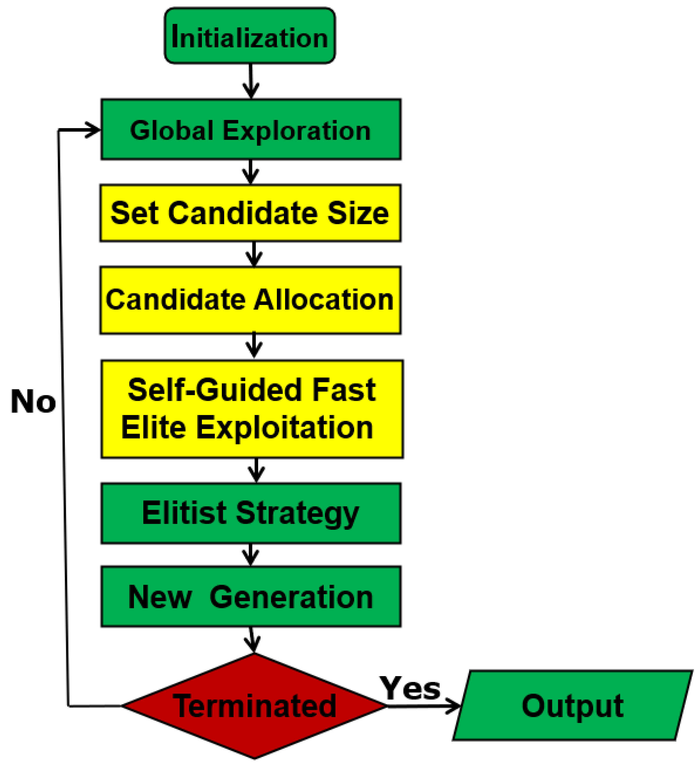
Figure 1 illustrates the framework of NSGA-II-BnF, composed of initialization, genetic population-based exploration, elitist exploitation intensity mechanism, crowding distance-based allocation procedures, self-guided fast symmetry exploitation procedures. The algorithm ends when the termination condition is satisfied.
As the pseudo-code depicted in Algorithm 1, we first set the necessary parameters at the first line. The algorithm starts with initializing the population containing N individuals at line 1 to line 6. We then perform the classic population-based exploration procedures (e.g., evaluation, non-dominated sorting, crowding distance calculation, genetic operation) at line 9 to line 16.
These steps result in a population set P with approximately 2N individuals. At line 17, we apply our proposed crowding distance-based resource allocation strategy to elites in the population P. There are two steps: (1) set the size of the candidate group using our proposed mechanism and (2) allocate resources by individuals’ crowding distance (the details of maintained steps will be shown in the following Sections). At line 18, we obtain an composed of elites and the resources they were allocated. Next, at line 19, we activate our proposed fast self-guided elite exploitation procedure based on the information in , use the computational resources they were allocated to generate their neighbors, and set the generated neighbors to set K at line 20. Finally, we combine set K into set P at line 26, and select the best N individuals as the next generation of the population from line 27 to line 29. The algorithm ends when the termination condition is satisfied.
| Algorithm 1 Main Loop of NSGA-II-BnF |
| Input: N, k, r, |
| Output: population set PInitialize: population set P |
| 1: for each do |
| 2: Evaluation; |
| 3: Non-Dominated sort; |
| 4: Crowding distance; |
| 5: end for |
| 6: =1; |
| 7: while do |
| 8: genetic procedures to population P; |
| 9: obtain an offspring set Q; |
| 10: for each do |
| 11: Evaluation; |
| 12: Non-Dominated sort; |
| 13: Crowding distance; |
| 14: end for |
| 15: ; |
| 16: do Non-dominated sort operate to set P; |
| 17: biased resource allocation strategy; //(Algorithm 2); |
| 18: obtain an archive D; |
| 19: do self-guided fast symmetry individual exploitation to archive D;//(Algorithm 3); |
| 20: obtain a set K of generated neighbors; |
| 21: for each do |
| 22: Evaluation; |
| 23: Non-Dominated sort; |
| 24: Crowding distance; |
| 25: end for |
| 26: ; |
| 27: do Non-dominated sort operate to set P; |
| 28: do elite strategy to set P; |
| 29: =+1; |
| 30: end while |
| 31: obtain a population set P; |
3.1. Biased Elite Allocation Strategy
Assume that individual exploitation is like a chance for reproduction. According to classic Social Darwinism, the fittest survive. Maybe we can understand the theory in this way: the fittest is expected to gain more resources in a resource-insufficient environment to ensure the positive evolution of the population.
Inspired by this theory, we propose an “elite only” strategy called the elite exploitation strategy. Which offer exploitation opportunity to a group of the best individuals in the population.
The central concept of this strategy is two-fold. First, decision makers may adjust the bias factor k value to control the candidate group’s size with their preference by our designed mechanism, and control the total consumption of computational resources during the exploitation procedures. Second, after we confirm the size of the candidate group, we allocate the exploitation opportunities appropriately to individuals, by proposing a crowding distance-based roulette, which also maintains diversity.
The pseudo-code of the biased elite allocation strategy is depicted in Algorithm 2. In the first line, we have a population set with about 2N individuals, and a bias factor, which is set at the beginning of Algorithm 1. From line 1 to line 5, we copy the best individuals (i.e., elites), which are in the first level of Non-Dominated ranking, into a subset T, called the candidate group. We then calculate crowding distance-based cumulative probability of each individual in subset T at line 7 to line 9. From line 11 to line 19, the crowding distance-based roulette procedures select the candidates from set T into , according to their value of crowding distance-based cumulative probability, the larger the crowding distance, the higher the probability of being selected. Note that individuals may be selected repeatedly.
| Algorithm 2 Biased Elite Allocation Strategy |
| Input: set P, k |
| Output: |
| 1: for each do |
| 2: if Non-Dominated rank of ==1 then |
| 3: ; |
| 4: end if |
| 5: end for |
| 6: for each do |
| 7: calculate the cumulative probability by Equations (2) and (3); |
| 8: end for |
| 9: m=1; |
| 10: while do |
| 11: h=rand(1); |
| 12: if then |
| 13: ; |
| 14: else |
| 15: find that makes holds; |
| 16: ; |
| 17: end if |
| 18: +1; |
| 19: end while |
| 20: obtain an ; |
More details are defined in the following two subsections: (1) management of quota and (2) quota allocation.
3.1.1. The Size of Candidate Group
In the first version of NSGA-II-BnF, the fast exploitation operator that was described in Section 3.2 was applied to every non-dominated individual called “elite” in the population, and a significant improvement of effectiveness was obtained.
However, with the progress of the evolutionary process, more and more individuals in the population are non-dominated, the growing number of elites causes the exploitation operator to consume significant computational resources, and the point is, sometimes the algorithm might face some insufficient computational resource circumstances. So, for a better applicability of the algorithm, management of the size of the candidate group is required.
Thus, we propose a manual mechanism that allows decision makers to manage the exploitation intensity with their preference. This mechanism functions by adjusting the maximum candidate group size, and is defined as
where k is a bias factor and input manually by decision makers at the beginning of Algorithm 1, N is the size of the population, and this equation denotes there will be members in the following exploitation procedure.
It is evident that the variable k has a positive correlation with the maximum candidate size, and decision makers can set the k value according to their preference.
3.1.2. Allocation Procedure
Roulette is a classic probabilistic-based selection method. It uses the individual’s proportion to the whole population to denote the probability of the individual being selected. We maintain diversity by proposing crowding distance-based roulette, which uses crowding distance as an indicator to calculate the selected probability of the elite from the set T.
In a word, the larger the crowding distance, the higher the probability of being selected. The main steps are as follows.
- (1)
- Apply crowding distance-based normalization calculated as below to individuals in set T.where is the i-th individual of set T, is the probability of an individual being selected, is the crowding distance of , and t is the number of individuals of set T.
- (2)
- Calculate the cumulative probability of each defined as
- (3)
- Generate a random number h in [0,1].
- (4)
- If , save individual at ; otherwise, find the individual , which makes holds, and save individual at .
- (5)
- Repeat steps (3) and (4) until there are members in .
Note that individuals may be selected repeatedly. At the end of this part, we obtain with members.
3.2. Self-Guided Fast Symmetry Individual Exploitation Approach
A widely-used individual exploitation system [40] in other hybrid algorithms is as follows:
where is the new j-th dimension generated by Equation (4), is the j-th dimension of , and is random turbulence. Equation (4) is a classic turbulence system, but with a defect: with the progress of evolution, the data in each dimension will be minimal, approximately in the range of –. This randomly created is always on another order of magnitude, this is a necessary method of exploring the solution space for an independent algorithm. However, as part of the individual exploitation procedure, it produces many meaningless neighbors, which is generally seen as a waste of computational resources.
We propose a self-guided fast symmetry individual exploitation strategy to solve this problem. We introduce this strategy in two subsections: (1) self-guided individual exploitation system and (2) tanh-based turbulence operator.
More details are described in Algorithm 3. At the first line, we obtain several variables set at the beginning of the algorithm. Variable r is the number of generated neighbor(s) of each member in . From line 6 to line 8, we calculate the turbulence v, and pick a random j-th dimension of . If the j-th dimension value is not 0, then we calculate the new value for j-th dimension at line 10, then we obtain a new neighbor of with a new j-th dimension from line 11 to line 12. Then put the new neighbor into set K at line 13. At the end of this part, we obtain a set K with neighbors.
| Algorithm 3 Self-guided fast symmetry individual exploitation |
| Input: n, archive D, a, b, r, |
| Output: set K |
| 1: Initialize: variable s, i; |
| 2: for each member in do; |
| 3: s=1; |
| 4: for do; |
| 5: l=round(rand(1)*())); |
| 6: calculate turbulence v by l and Equation (7); |
| 7: j=randperm(n,1); |
| 8: if then |
| 9: calculate new dimension by Equation (5); |
| 10: replace the by ; |
| 11: obtain a neighbor of ; |
| 12: ; |
| 13: else |
| 14: goto line 6; |
| 15: end if |
| 16: ; |
| 17: end for |
| 18: end for |
| 19: obtain a set K of neighbors; |
3.2.1. Self-Guided Individual Exploitation System
This system uses the meme [35] that contains information on the evolution stage to guide individual exploitation procedures. Our proposed approach is as follows.
where v is the turbulence introduced in Section 3.2.2. Equation (5) denotes that as the evolution progresses, the data in each dimension decreases and the created turbulence decreases, such that the newly generated neighbors are always in the proper range.
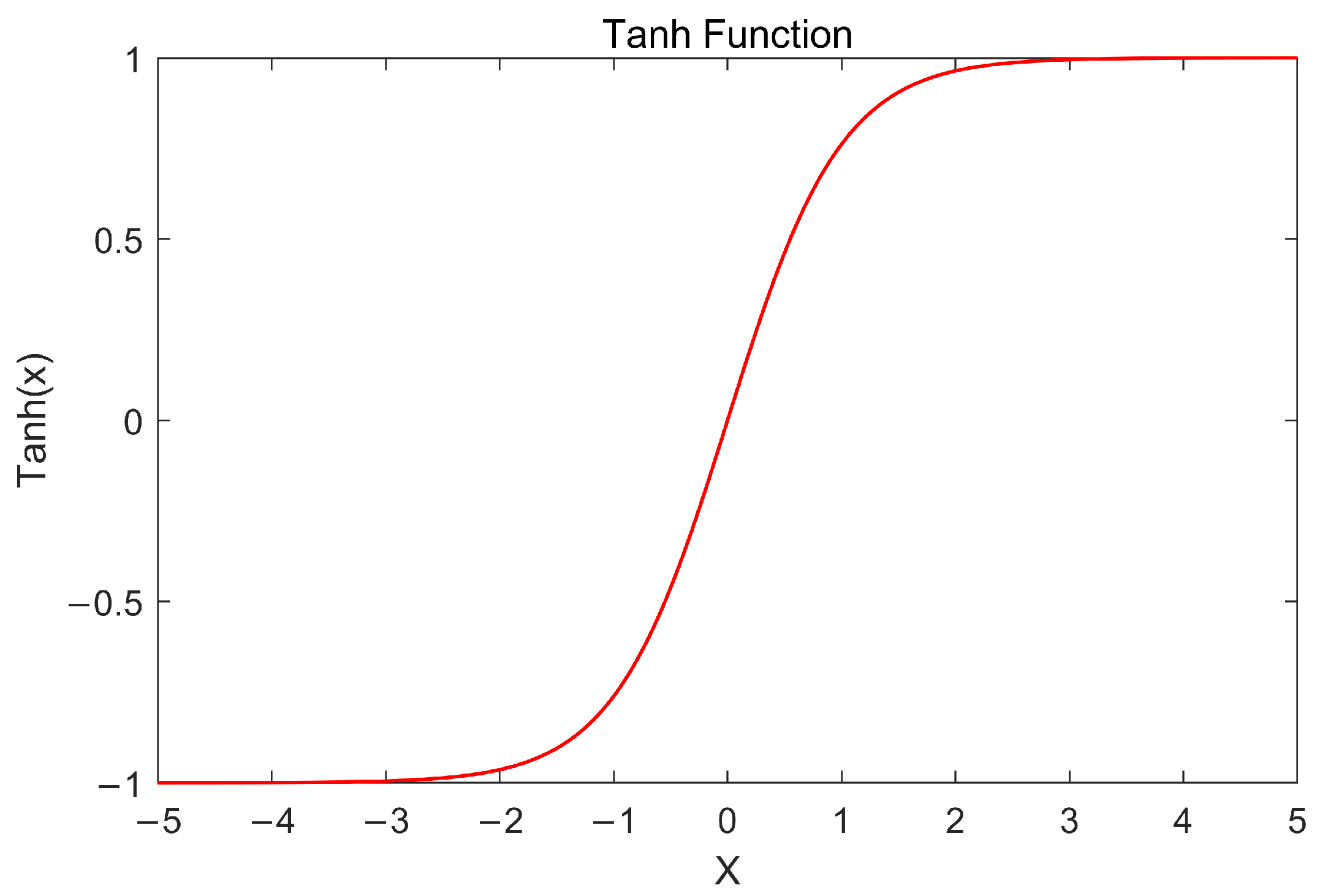
3.2.2. Tanh-Based Exploitation Operator
In mathematics, the hyperbolic tangent ’tanh’ [41] is derived from the classic hyperbolic function. It has a regular and opposite value interval within a specific symmetry domain which is shown in Figure 2, and makes it suitable as a turbulence operator. Its equation is as follows.
The procedure of generating neighbors of a candidate is depicted as follows.
- (1)
- Generate a set L with r random number(s), the value of which is in the interval ; for an example, we set ;
- (2)
- For each , calculate as below, which results in the set of turbulence values .
- (3)
- Select j-th dimension of randomly.
- (4)
- After obtaining the turbulence, we use Equation (5) to generate the new j-th dimension , then, we generate neighbors of defined aswhere r is the number of neighbors and set in the beginning of the algorithm, is the s-th neighbor of and is the s-th element of V. This equation denotes that the s-th neighbor of is with a new j-th dimension.
Due to the features of tanh function, the intensity of turbulence is controlled by range , because the values of are evenly distributed in , such that a broader range of indicates more l values far away from the origin, which makes the v value likely to be larger, and cause a greater turbulence intensity.
4. Experiment
4.1. Test Problems
We selected 36 widely-used test problems to compare our proposed algorithm’s performance with nine other competitive algorithms. The UF1–UF10 is proposed for a set of CEC2009 benchmark problems, with a very complex true PF. Likewise, test problems CF1–CF10, WFG1–WFG9, and DTLZ1–DTLZ7 are also challenging. We set WFGs, UF1–UF7, and CF1–7 with two objectives and DTLZs, CF8–10, and UF8–UF10 with three objectives.
4.2. Indicators
We use the two most common performance indicators (i.e., inverted generational distance (IGD) [42] and hypervolume (HV) [43]) to measure our proposed algorithm and compare it with other algorithms.
IGD is a comprehensive performance evaluation index. It primarily evaluates the algorithm’s convergence and distribution performance by calculating the sum of the minimum distances between each point (individual) on the real PF and the set of individuals obtained by the algorithm.
The HV indicator calculates the volume of the region that was bounded by the non-dominated solution set and the reference points.
The value of HV is positively correlated with the performance of the algorithm. For all problems with two objectives, the reference points are set as (2.0,2.0). For all problems with three objectives, the reference points are set as (2.0,2.0,2.0).
4.3. Experiment Settings
Four NSGA-IIs (NSGA-IIconflict, rNSGA-II, RPDNSGA-II [24], NSGAII-SDR) and four classic MOEAs (SMOPSO, SPEA-II, MOEA/D-DE, dMOPSO) are used for the performance comparison.
The relative parameters of the algorithms are summarized in Table 1. The population size N is set to 200, k is the bias factor set by users, and r is the number of neighbors of each candidate. and are the crossover probability and mutation probability, respectively. is the number of set reference points, is the number of set weight vectors for each preferred point, and is the non-r-dominance threshold. is the number of subspaces, and is the number of cycles. T is the size of the neighborhood regarding the weight vectors, and are the probability of selecting parents from T neighbors and the maximum number of parent solutions replaced by each child solution, respectively. , , and are the parameters in the velocity update equation for MOPSOs.
For test problems DTLZ1–DTLZ7 and WFG1-WFG9, we set the number of function evaluations to 50,000. For test problems UF1-UF10 and CF1-CF10, we set the number of function evaluations to 300,000. For fairness, we set the dimension of individuals to 20 for each problem.
All algorithms executed 30 independent runs on each problem under the same hardware environment. The mean values and standards deviations of IGD and HV after 30 runs were collected for comparison. Moreover, Wilcoxon’s rank-sum test was calculated for a statistically sound conclusion, with a significance level of . In the following tables, the symbols “+”, “−”, and “=” indicate that the results of competitors are significantly better than, worse than, and similar to, respectively, the results of NSGA-II-BnF, and the best results on each test problems are shown in bold.
4.4. Comparison among NSGA-II-BnF and Four NSGA-II Series Algorithms
We selected four peer NSGA-II-BnF algorithms (NSGA-IIconflict, rNSGA-II, RPDNSGA -II, NSGAII-SDR) to compare the performance on 36 challenging MOPs. The results of the IGD indicator of each algorithm after 30 independent runs are depicted in Table 2.
In Table 2, it is evident that our proposed NSGA-II-BnF obtained high performance based on the mean IGD values, with the best results in 18 of 36 cases. Furthermore, NSGA-IIconflict, rNSGA-II, RPDNSGA-II, and NSGAII-SDR obtained 2, 3, 9, and 4 best results, respectively. For WFG series problems, NSGA-II-BnF exhibited superior performance, obtaining the best results in 7 of 9 cases, NSGAII-SDR obtained the best results on WFG8, and NSGA-IIconflict obtained the best results on WFG6. On UF series MOPs, the performance of NSGA-II-BnF was like its peer algorithms, where NSGA-II-BnF, NSGAII-SDR, RPDNSGA-II, rNSGA-II, and NSGA-IIconflict obtained best results in 3, 2, 4, 1, and 0 of 10 cases, respectively. Peer algorithms experienced difficulties when facing CF-series problems, however, NSGA-II-BnF obtained the best results in 7 of 10 cases, which confirmed our proposed individual exploitation operator’s effectiveness and the necessity of the individual-based exploitation strategy to maintain diversity when tackling complex MOPs.
The last row of Table 2 demonstrates the total number of problems in which NSGA-II-BnF was better than , similar to , and worse than the compared algorithms. These statistics demonstrate that NSGA-II-BnF is superior to NSGA-IIconflict, rNSGA-II, RPDNSGA-II, and NSGAII-SDR in 27, 28, 26, and 24 cases among 36 test problems, and NSGA-II-BnF is only worse than NSGA-IIconflict, rNSGA-II, RPDNSGA-II, and NSGAII-SDR on 1, 3, 8, and 3 test problems, respectively.
We can learn from Table 2 that our proposed NSGA-II-BnF is significantly superior to its peer algorithms for the IGD indicator. Furthermore, we consider this superior performance the result of our effective resource allocation strategy, enhancing convergence performance when solving MOPs with usual complexity.
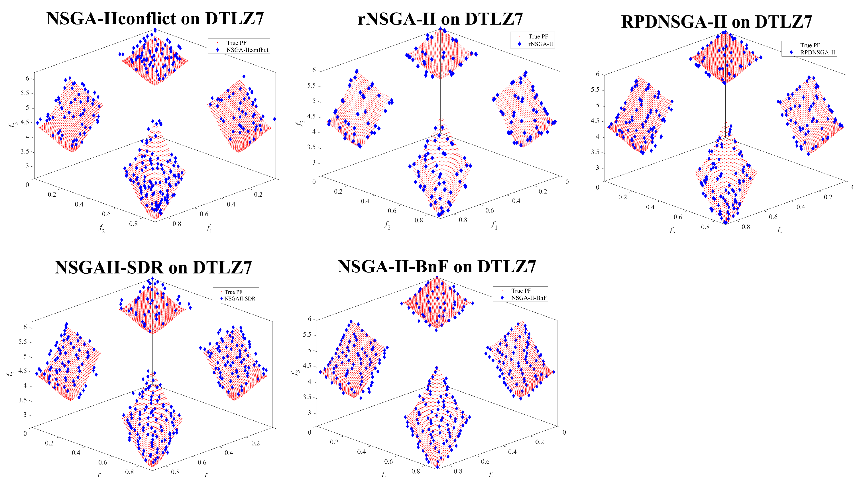
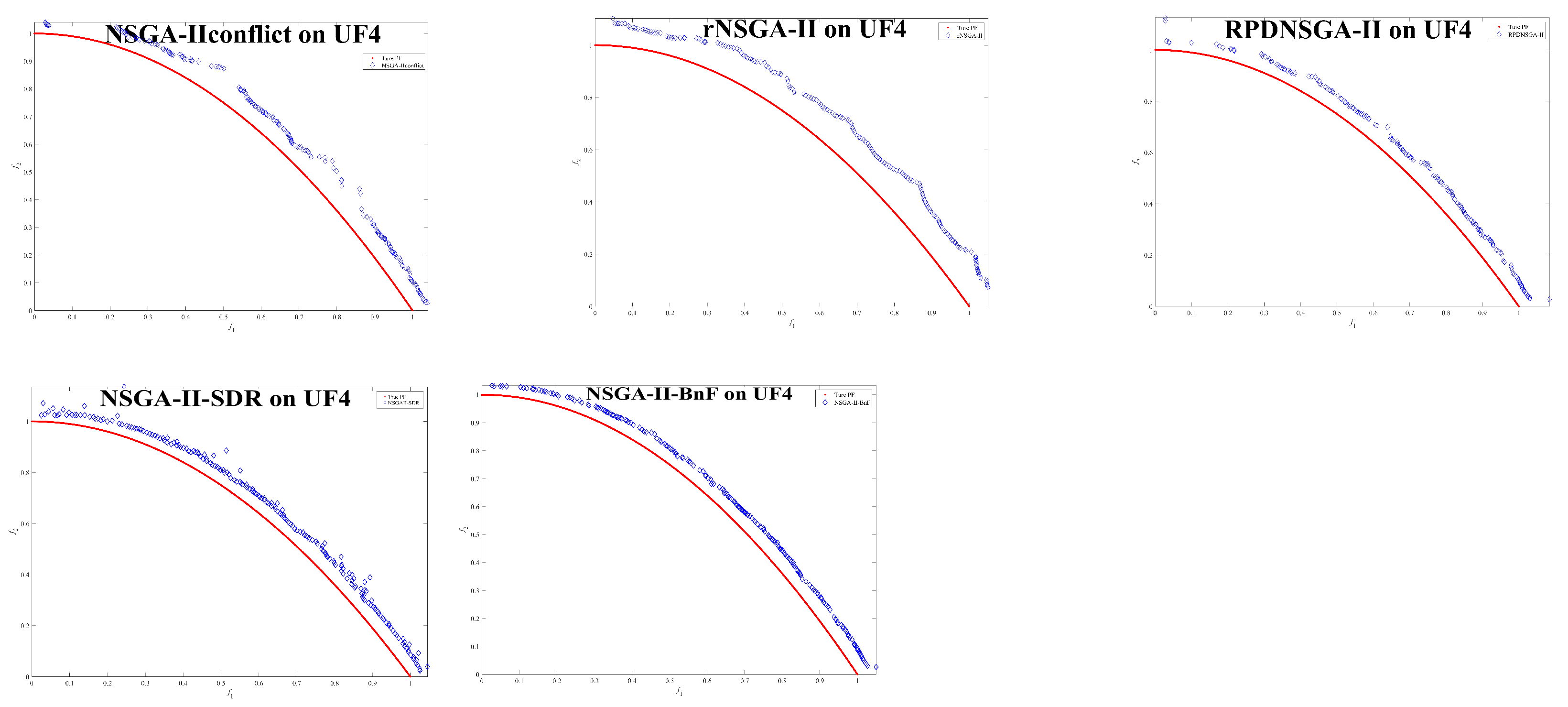
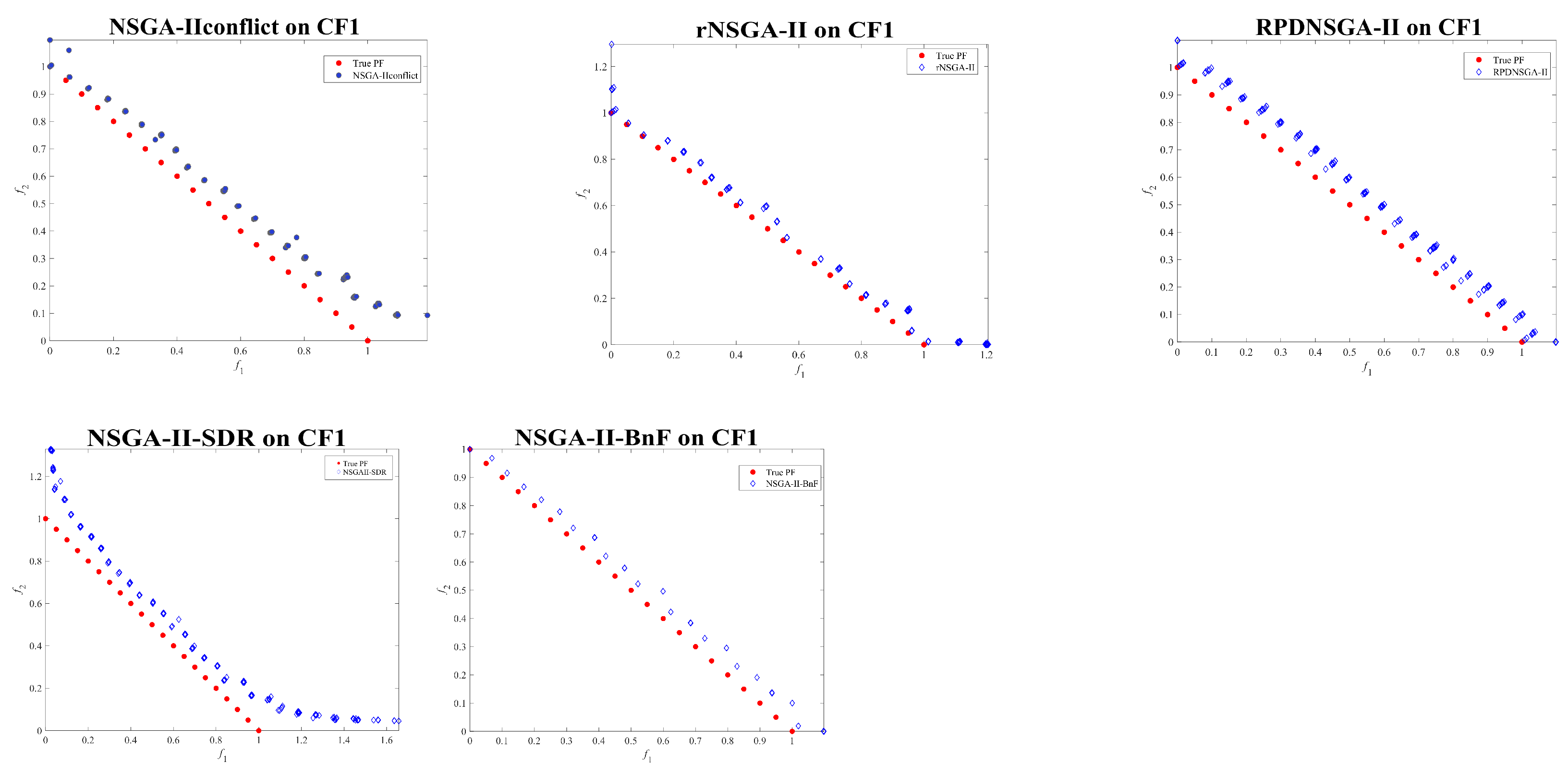
We support our conclusion by presenting several examples of obtained final approximated non-dominated solutions in Figure 3, Figure 4, Figure 5, Figure 6 and Figure 7. These results indicate that NSGA-II-BnF always has superior convergence performance and diversity, resulting in a smoother front than its peer algorithms.
The results of the comparison among NSGA-II-BnF and its peers on the HV indicator are depicted in Table 3. The comparison for HV value is similar to IGD values. NSGA-II-BnF obtained 19 of 36 best results. Furthermore, NSGA-IIconflict, rNSGA-II, RPDNSGA-II, and NSGAII-SDR obtained 1, 2, 7, and 7 best results, respectively. The last row of Table 3 presents NSGA-II-BnF outperforms NSGA-IIconflict, rNSGA-II, RPDNSGA-II, and NSGAII-SDR for the Wilcoxon’s rank-sum test on 29, 28, 28, and 19 test problems, respectively. Thus, we can conclude that our proposed NSGA-II-BnF has special competitiveness when facing the MOPs with complex PF.
4.5. Comparison Among NSGA-II-BnF and Four Classic Algorithms
We selected four widely-used and competitive algorithms (SPEA-II, MOEA/D-DE, SMPSO, and dMOPSO) to compare with our proposed NAGS-II-BnF. Each algorithm executed 30 independent runs on the test problems. We also selected IGD and HV as the indicators.
The results of the comparison for the IGD value are depicted in Table 4. Our proposed NSGA-II-BnF obtained 23 of 36 best cases, and SPEA-II, MOEA/D-DE, SMOPSO, and dMOPSO obtained 7, 1, 2, and 3 best cases, respectively. For DTLZ series problems, NSGA-II-BNF obtained 4 of 7 best results, compared with SPEA-II, MOEA/D-DE, SMOPSO, and dMOPSO obtained 1, 1, 0, 1 best results. Especially, For UF series problems, NSGA-II-BNF obtained 9 of 10 best results, compared with SPEA-II, which obtained one best result.
Furthermore, the last row reveals that NSGA-II-BnF had a better performance on 24, 27, 29, and 29 test problems for Wilcoxon’s rank-sum test compared to SPEA-II, MOEA/D-DE, SMOPSO, and dMOPSO, respectively. We can see from Table 4, our proposed NSGA-II-BnF shows better performance on IGD values than four competitive algorithms on most of the test problems.
The results of the comparison with the HV value are depicted in Table 5. Our proposed NSGA-II-BnF obtained 21 of 36 best cases, and SPEA-II, MOEA/D-DE, SMOPSO, and dMOPSO obtained 7, 4, 1, and 3 best cases, respectively.
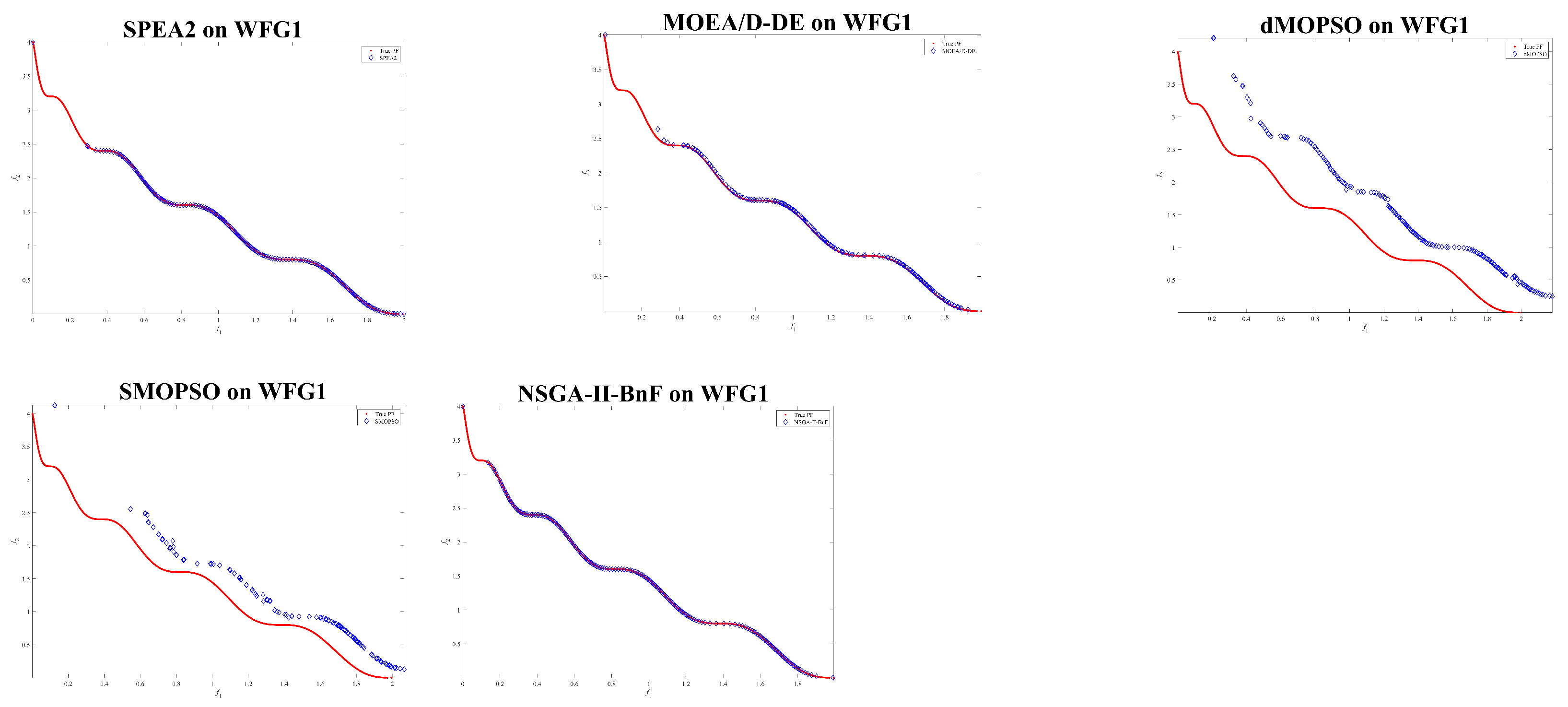
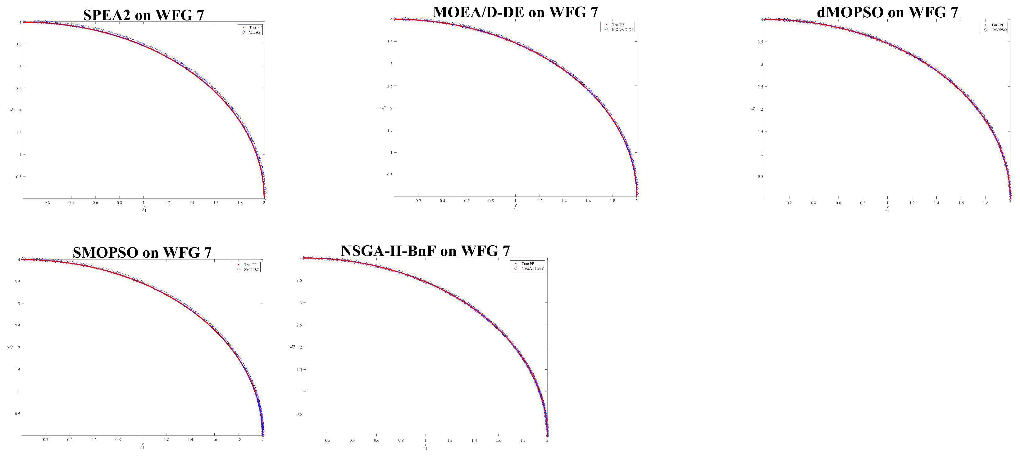
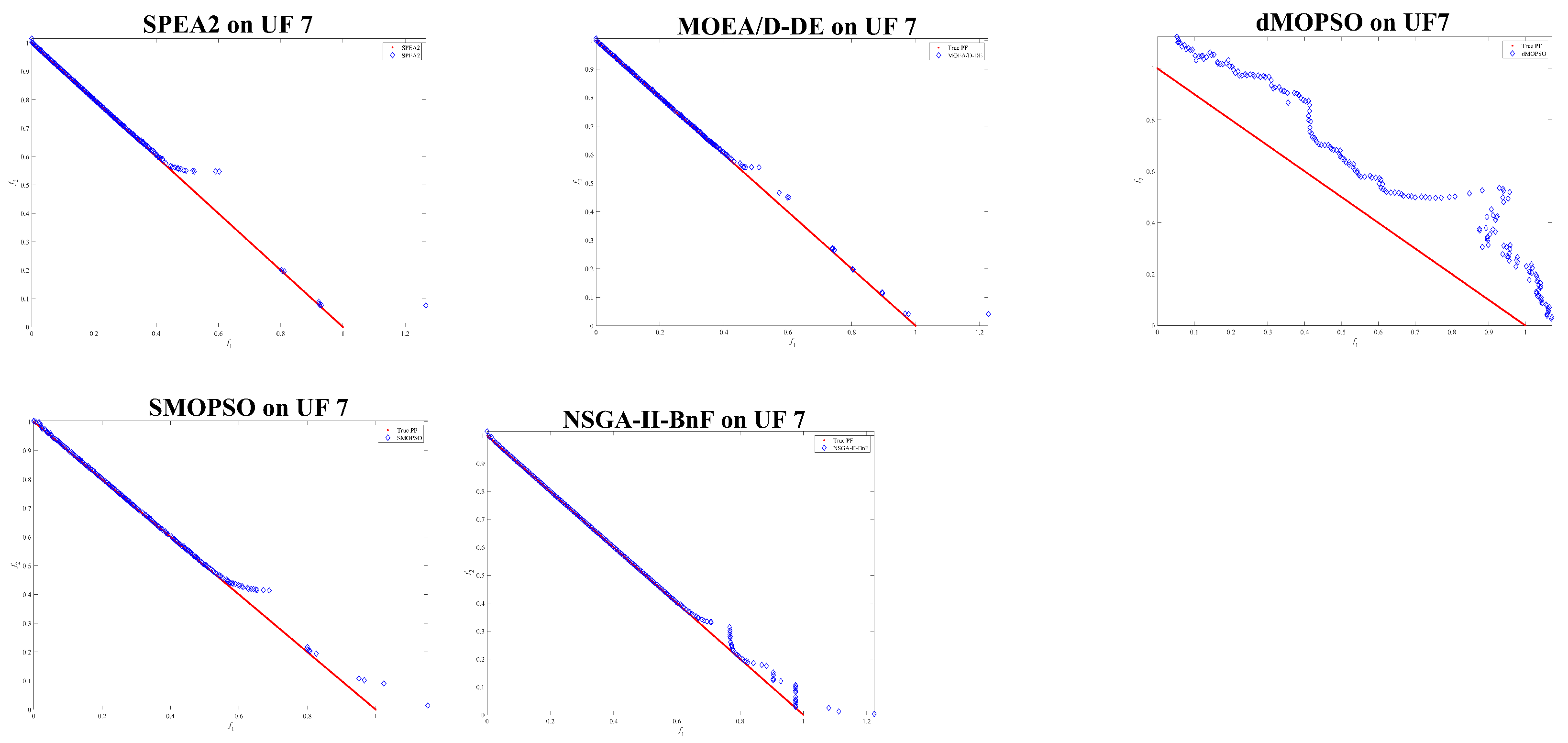
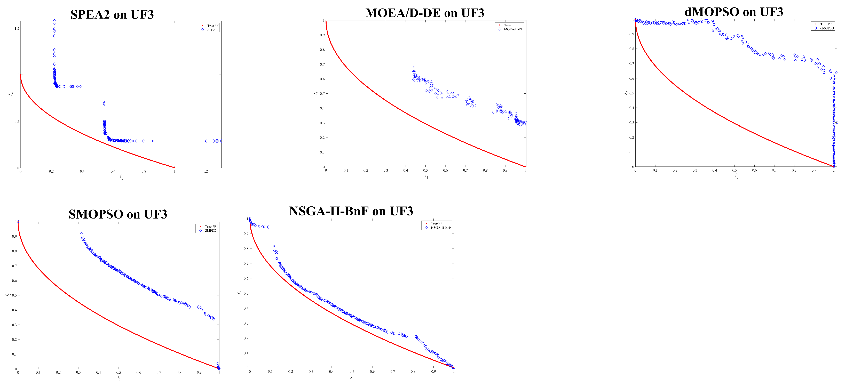
Moreover, the last row demonstrates that NSGA-II-BnF had the best performance on 23, 24, 30, and 27 test problems for Wilcoxon’s rank-sum test compared to SPEA-II, MOEA/D-DE, SMOPSO, and dMOPSO, respectively. We can see from Table 5, our proposed NSGA-II-BnF shows better performance on HV values on most of the test problems than four competitive algorithms. To visually show the advantage of NSGA-II-BnF, we plotted the comparison of NSGA-II-BnF with SPEA-II, MOEA/D-DE, SMOPSO, and dMOPSO on WGF1, WFG7, UF3, UF7 CF2, as shown in Figure 8, Figure 9, Figure 10, Figure 11 and Figure 12. These figures demonstrate that NSGA-II-BnF always obtained a smoother PF and greater convergence than the other four algorithms.
Based on the discussions above, we can draw this conclusion that our proposed NSGA-II-BnF always outperformed the compared algorithms reflected in the graphs as smoother, more even, and closer to the true PF than the compared algorithms. We consider these advantages and outstanding performance as the successful result of our proposed resource allocation strategy and individual exploitation strategy.
4.6. Comparison between NSGA-II-BnF and NSGA-II
In this part, we compared the original NSGA-II and NSGA-II with the biased resource allocation strategy and fast individual exploitation strategy to determine the extent to which our proposed algorithm improved the original algorithm.
Each algorithm executed 30 independent runs on 36 test problems; the IGD and HV values are depicted in Table 6.
Table 6 presents that on the IGD indicator, our proposed NSGA-II-BnF obtained 28 of 36 best cases compared with 8 of 36 cases that NSGA-II obtained, and the last row reveals that NSGA-II-BnF obtained 17 of 36 best cases and 15 of 36 similar cases for Wilcoxon’s rank-sum test.
The comparison of HV values is similar. We obtained 27 of 36 best cases, and NSGA-II obtained 9 of 36 cases. The last row reveals that NSGA-II-BnF obtained 19 of 36 best cases and 12 of 36 similar cases for Wilcoxon’s rank-sum test. Thus, we can conclude that our two proposed strategies’ effectiveness has been confirmed from the above experiments.
5. Conclusions and Future Works
In this paper, we explore the combination of a mathematical method and EMO approach, and propose an improved version of NSGA-II with a biased elite exploitation strategy, called NSGA-II-BnF. During the evolution process, the resource allocation strategy selects candidates by our proposed crowd distance based roulette, which enhances our algorithm’s diversity. Then, a novel exploitation system based on a self-guided approach and the hyperbolic tangent function based local search operator is performed to improve convergence performance. Meanwhile, for emphasizing the algorithm’s applicability, we propose a mechanism that allows decision makers to control the exploitation intensity with their preference.
The proposed NSGA-II-BnF demonstrated outstanding performance on convergence and diversity in the simulation experiment when facing different MOPs compared with other competitive algorithms. Meanwhile, there are still some areas that can be improved in our work. For example, in this work, we apply elite exploitation in every generation, for better efficiency, the elite exploitation strategy may be activated periodically; moreover, for many-objective optimization problems, the proposed exploitation operator may not give enough pressure of evolution, thus, a more targeted local search operator should be proposed.
In the future, we will consider proposing an elite exploitation activation mechanism to improve efficiency, learn from the experience of the existing works, design a better exploitation operator for many-objective problems, and use our algorithm to solve real-world problems.
Author Contributions
Conceptualization, W.L. and K.Z.; data curation, W.L., Y.G., K.Z. and J.L.; funding acquisition, Y.G.; methodology, J.Z.; project administration, Y.G. and J.L.; resources, Y.G.; software, J.Z.; supervision, Y.G. and J.Z.; writing—original draft, W.L. and J.L.; writing—review and editing, W.L. and K.Z. All authors have read and agreed to the published version of the manuscript.
Funding
This work was supported in part by the National Key R&D Program of China (No. 2019YFB1404700).
Institutional Review Board Statement
Not applicable.
Informed Consent Statement
Not applicable.
Data Availability Statement
Data sharing not applicable.
Acknowledgments
This work was supported in part by the National Key Research and Development Program of China under Grant 2019YFB1404700.
Conflicts of Interest
The authors declare no conflict of interest.
References
- Miettinen, K. Nonlinear Multiobjective Optimization; Kluwer: Boston, MA, USA, 1999. [Google Scholar]
- Liu, Y.; Qin, H.; Zhang, Z.; Yao, L.; Wang, C.; Mo, L.; Ouyang, S.; Li, J. A region search evolutionary algorithm for many-objective optimization. Inf. Sci. 2019, 488, 19–40. [Google Scholar] [CrossRef]
- Cui, Z.; Zhang, J.; Chang, Y.; Cai, X.; Zhang, W. Improved NSGA-III with selection-and-elimination operator. Swarm Evol. Comput. 2019, 49, 23–33. [Google Scholar] [CrossRef]
- Zitzler, E.; Laumanns, M.; Thiele, L. Spea2: Improving the strength pareto evolutionary algorithm. TIK-Report Computer Engineering and Communication Networks Lab(TIK), Swiss Federal Institute of Technology (ETH) Zurich, ETH Zentrum, Gloriastrasse 35, CH-8092 Zurich, Switzerland, Sept. 2001, 103. Available online: https://0-doi-org.brum.beds.ac.uk/10.3929/ethz-a-004284029 (accessed on 30 December 2020).
- Deb, K.; Pratap, A.; Agarwal, S.; Meyarivan, T. A fast and elitist multiobjective genetic algorithm: Nsga-ii. IEEE Trans. Evol. Comput. 2002, 6, 182–197. [Google Scholar] [CrossRef] [Green Version]
- Tian, Y.; Cheng, R.; Zhang, X. A Strengthened Dominance Relation Considering Convergence and Diversity for Evolutionary Many-Objective Optimization. IEEE Trans. Evol. Comput. 2018, 23, 331–345. [Google Scholar] [CrossRef] [Green Version]
- Xia, X.; Gui, L. An Expanded Particle Swarm Optimization Based on Multi-Exemplar and Forgetting Ability. Inf. Sci. 2020, 508, 105–120. [Google Scholar] [CrossRef]
- Xu, G.; Cui, Q.; Shi, X. Particle swarm optimization based on dimensional learning strategy. Swarm Evol. Comput. 2019, 45, 33–51. [Google Scholar] [CrossRef]
- Nebro, A.J.; Durillo, J.J.; Garcia-Nieto, J.; Coello, C.A.C.; Alba, E. Smpso: A new pso-based metaheuristic for multi-objective optimization. In Proceedings of the IEEE Symposium on Computational Intelligence in Multi-Criteria Decision-Making, Nashville, TN, USA, 30 March–2 April 2009; pp. 66–73. [Google Scholar]
- Liu, Y.; Zhu, N.; Li, K.; Li, M.; Zheng, J.; Li, K. An angle dominance criterion for evolutionary many-objective optimization. Inf. Sci. 2020, 509, 376–399. [Google Scholar] [CrossRef]
- Said, L.B.; Bechikh, S.; Ghédira, K. The r-Dominance: A New Dominance Relation for Interactive Evolutionary Multicriteria Decision Making. IEEE Trans. Evol. Comput. 2010, 14, 801–818. [Google Scholar] [CrossRef]
- Mirjalili, S.; Saremi, S.; Mirjalili, S.M.; Coelho, L.D.S. Multiobjective grey wolf optimizer: A novel algorithm for multi-criterion optimization. Expert Syst. Appl. 2016, 47, 106–119. [Google Scholar] [CrossRef]
- Liang, Z.; Luo, T.; Hu, K.; Ma, X.; Zhu, Z. An Indicator-Based Many-Objective Evolutionary Algorithm With Boundary Protection. IEEE Trans. Evol. Comput. 2020, 99, 1–14. [Google Scholar] [CrossRef]
- Hong, W.; Tang, K.; Zhou, A.; Ishibuchi, H.; Yao, X. A scalable indicator-based evolutionary algorithm for large-scale multiobjective optimization. IEEE Trans. Evol. Comput. 2018, 23, 525–537. [Google Scholar] [CrossRef]
- Tian, Y.; Cheng, R.; Zhang, X.; Cheng, F.; Jin, Y. An indicator-based multiobjective evolutionary algorithm with reference point adaptation for better versatility. IEEE Trans. Evol. Comput. 2017, 22, 609–622. [Google Scholar] [CrossRef] [Green Version]
- Silvestre, M.L.D.; Graditi, G.; Sanseverino, E.R. A generalized framework for optimal sizing of distributed energy resources in microgrids using an indicator-based swarm approach. IEEE Trans. Ind. Inform. 2013, 10, 152–162. [Google Scholar] [CrossRef]
- Li, F.; Cheng, R.; Liu, J.; Jin, Y. A two-stage r2 indicator based evolutionary algorithm for many-objective optimization. Appl. Soft Comput. 2018, 67, 245–260. [Google Scholar] [CrossRef] [Green Version]
- Sun, Y.; Yen, G.G.; Yi, Z. IGD Indicator-Based Evolutionary Algorithm for Many-Objective Optimization Problems. IEEE Trans. Evol. Comput. 2018, 23, 173–187. [Google Scholar] [CrossRef] [Green Version]
- Pamulapati, T.; Mallipeddi, R.; Nagaratnam, P. ISDE—An Indicator for Multi and Many-Objective Optimization. IEEE Trans. Evol. Comput. 2018, 23, 346–352. [Google Scholar] [CrossRef]
- Zhou, A.; Zhang, Q. Are all the subproblems equally important? resource allocation in decomposition-based multiobjective evolutionary algorithms. IEEE Trans. Evol. Comput. 2015, 20, 52–64. [Google Scholar] [CrossRef]
- Jaimes, A.L.; Coello, C.A.C.; Aguirre, H.; Tanaka, K. Objective space partitioning using conflict information for solving manyobjective problems. Inf. Sci. 2014, 268, 305–327. [Google Scholar] [CrossRef]
- Lin, Q.; Jin, G.; Ma, Y.; Wong, K.; Coello, C.A.C.; Li, J.; Chen, J.; Zhang, J. A diversity-enhanced resource allocation strategy for decomposition-based multiobjective evolutionary algorithm. IEEE Trans. Cybern. 2018, 48, 2388–2401. [Google Scholar]
- Li, H.; Zhang, Q. Multiobjective optimization problems with complicated pareto sets, moea/d and nsga-ii. IEEE Trans. Evol. Comput. 2008, 13, 284–302. [Google Scholar] [CrossRef]
- Elarbi, M.; Bechikh, S. A new decomposition-based NSGA-II for many-objective optimization. IEEE Trans. Syst. Man Cybern. Syst. 2017, 48, 1191–1210. [Google Scholar] [CrossRef]
- Ma, X.; Zhang, Q.; Yang, J.; Zhu, Z.; Tian, G. On tchebycheff decomposition approaches for multiobjective evolutionary optimization. IEEE Trans. Evol. Comput. 2018, 22, 226–244. [Google Scholar] [CrossRef]
- Han, D.; Du, W.; Du, W.; Jin, Y.; Wu, C. An adaptive decomposition-based evolutionary algorithm for many-objective optimization. Inf. Sci. 2019, 491, 204–222. [Google Scholar] [CrossRef]
- Zhang, Q.; Liu, W.; Li, H. The performance of a new version of moea/d on cec09 unconstrained mop test instances. In Proceedings of the 2009 IEEE Congress on Evolutionary Computation, Trondheim, Norway, 18–21 May 2009; pp. 203–208. [Google Scholar]
- Wang, L.; Zhang, Q.; Zhou, A.; Gong, M.; Jiao, L. Constrained subproblems in a decomposition-based multiobjective evolutionary algorithm. IEEE Trans. Evol. Comput. 2015, 20, 475–480. [Google Scholar] [CrossRef]
- Zhang, J.; Zhou, A.; Zhang, G. A multiobjective evolutionary algorithm based on decomposition and preselection. In Bio-Inspired Computing-Theories and Applications; Springer: Berlin/Heidelberg, Germany, 2015; pp. 631–642. [Google Scholar]
- Martínez, S.Z.; Coello, C.A.C. A multi-objective particle swarm optimizer based on decomposition. In Proceedings of the Conference on Genetic & Evolutionary, Dublin, Ireland, 12–16 June 2011; pp. 69–76. [Google Scholar]
- Trivedi, A.; Srinivasan, D.; Sanyal, K.; Ghosh, A. A Survey of Multiobjective Evolutionary Algorithms Based on Decomposition. IEEE Trans. Evol. Comput. 2016, 21, 440–462. [Google Scholar] [CrossRef]
- Xu, Q.; Xu, Z.; Ma, T. Short Survey and Challenges for Multiobjective Evolutionary Algorithms Based on Decomposition. In Proceedings of the 2019 International Conference on Computer, Information and Telecommunication Systems (CITS), Beijing, China, 28–31 August 2019. [Google Scholar]
- Crepinsek, M.; Liu, S.H.; Mernik, M. Exploration and exploitation in evolutionary algorithms: A survey. ACM Comput. Surv. 2013, 45, 1–33. [Google Scholar] [CrossRef]
- Mongus, D.; Repnik, B.; Mernik, M.; Žalik, B. A hybrid evolutionary algorithm for tuning a cloth-simulation model. Appl. Soft Comput. 2012, 12, 226–273. [Google Scholar] [CrossRef]
- Ong, Y.S.; Lim, M.H.; Chen, X. Memetic Computation - Past, Present & Future. IEEE Comput. Intell. Mag. 2010, 5, 24–31. [Google Scholar]
- Deb, K.; Thiele, L.; Laumanns, M.; Zitzler, E. Scalable Test Problems for Evolutionary Multiobjective Optimization. In Evolutionary Multiobjective Optimization; Springer: London, UK, 2006; pp. 105–145. [Google Scholar]
- Huband, S.; Barone, L.C.; While, L.; Hingston, P.F. A scalable multiobjective test problem toolkit. In Proceedings of the International Conference on Evolutionary Multi-Criterion Optimization, Guanajuato, Mexico, 9–11 March 2005; pp. 280–295. [Google Scholar]
- Zhang, Q.; Zhou, A.; Zhao, S.; Suganthan, P.N.; Liu, W.; Tiwari, S. Multiobjective optimization test instances for the CEC 2009 special session and competition. In Mechanical Engineering; American Society of Mechanical Engineers(ASME): Three Park Ave, NY, USA, 2009; pp. 1–30. [Google Scholar]
- Agrawal, R.B.; Deb, K.; Agrawal, R.B. Simulated binary crossover for continuous search space. Complex Syst. 1995, 9, 115–148. [Google Scholar]
- ling, W.; Dazhong, Z. Simulated annealing algorithm based on cauchy and gaussian distributed state generator. J. Tsinghua Univ. (Sci. Technol.) 2000, 40, 109–112. [Google Scholar]
- Yabe, T.; Aoki, T. A universal solver for hyperbolic equations by cubic-polynomial interpolation I. One-dimensional solver. Comput. Phys. Commun. 1991, 66, 219–232. [Google Scholar] [CrossRef]
- Bosman, P.A.N.; Thierens, D. The balance between proximity and diversity in multiobjective evolutionary algorithms. IEEE Trans. Evol. Comput. 2003, 7, 174–188. [Google Scholar] [CrossRef] [Green Version]
- Zitzler, E.; Thiele, L. Multi-objective evolutionary algorithms: A comparative case study and the strength Pareto approach. IEEE Trans. Evol. Comput. 1999, 3, 257–271. [Google Scholar] [CrossRef] [Green Version]
Figure 1.
The flow chart of NSGA-II-BnF.

Figure 2.
Figure of hyperbolic tangent function.

Figure 3.
Scatter plots of final Pareto optimal sets (PSs) of NSGA-II-BnF and the compared algorithms on WFG5.
Figure 3.
Scatter plots of final Pareto optimal sets (PSs) of NSGA-II-BnF and the compared algorithms on WFG5.

Figure 4.
Scatter plots of final PSs of NSGA-II-BnF and the compared algorithms on WFG6.

Figure 5.
Scatter plots of final PSs of NSGA-II-BnF and the compared algorithms on DTLZ7.

Figure 6.
Scatter plots of final PSs of NSGA-II-BnF and the compared algorithms on UF4.

Figure 7.
Scatter plots of final PSs of NSGA-II-BnF and the compared algorithms on CF1.

Figure 8.
Scatter plots of final PSs of NSGA-II-BnF and the compared algorithms on WFG1.

Figure 9.
Scatter plots of final PSs of NSGA-II-BnF and the compared algorithms on WFG7.

Figure 10.
Scatter plots of final PSs of NSGA-II-BnF and the compared algorithms on CF2.

Figure 11.
Scatter plots of final PSs of NSGA-II-BnF and the compared algorithms on UF7.

Figure 12.
Scatter plots of final PSs of NSGA-II-BnF and the compared algorithms on UF3.


Table 1.
Parameter settings.
| Algorithm | Parameter Settings |
|---|---|
| NSGA-II-conflict | |
| rNSGA-II | |
| RPDNSGA-II | |
| NSGA-II-SDR | |
| MOEA/D-DE | |
| dMOPSO | |
| SMOPSO | |
| SPEA-II | |
| NSGA-II-BnF |
Table 2.
Experimental results (mean and standard deviation) of inverted generational distance (IGD) values.
Table 2.
Experimental results (mean and standard deviation) of inverted generational distance (IGD) values.
| Problem | NSGA-IIconflict | rNSGA-II | RPDNSGA-II | NSGAII-SDR | NSGA-II-BnF |
|---|---|---|---|---|---|
| DTLZ1 | 9.9524 × 10 (5.42 × 10) − | + | 1.0742 × 10 (1.14 × 10) − | 2.1962 × 10 (5.68 × 10) − | 2.9848 × 10 (6.61 × 10) |
| DTLZ2 | + | 5.3578 × 10 (3.96 × 10) − | 8.1904 × 10 (1.46 × 10) − | 2.9394 × 10 (7.70 × 10) − | 2.0754 × 10 (1.65 × 10) |
| DTLZ3 | 1.1864 × 10 (2.46 × 10) = | = | 2.0767 × 10 (5.22 × 10) − | 2.3742 × 10 (6.63 × 10) − | 1.1138 × 10 (2.00 × 10) |
| DTLZ4 | 8.1915 × 10 (1.46 × 10) − | 3.0173 × 10 (1.28 × 10) − | + | 1.0502 × 10 (6.65 × 10) − | 2.6736 × 10 (1.35 × 10) |
| DTLZ5 | 8.1929 × 10 (1.46 × 10) − | 5.3366 × 10 (4.00 × 10) − | + | 2.9406 × 10 (4.72 × 10) − | 2.0743 × 10 (1.64 × 10) |
| DTLZ6 | 8.2086 × 10 (1.46 × 10) − | 1.2965 × 10 (4.41 × 10) − | + | 1.5183 × 10 (1.01 × 10) − | 2.0435 × 10 (1.12 × 10) |
| DTLZ7 | 8.6756 × 10 (1.55 × 10) − | 1.0854 × 10 (1.57 × 10) − | 1.5021 × 10 (2.11 × 10) − | 4.5382 × 10 (3.94 × 10) − | |
| WFG1 | 1.3503 × 10 (2.74 × 10) − | 3.2202 × 10 (7.66 × 10) − | 7.8765 × 10 (6.57 × 10) − | 1.4982 × 10 (1.27 × 10) − | |
| WFG2 | 1.1640 × 10 (1.09 × 10) − | 1.5311 × 10 (1.91 × 10) − | 1.1444 × 10 (3.26 × 10) − | 1.2612 × 10 (1.03 × 10) − | |
| WFG3 | 1.1179 × 10 (2.53 × 10) − | 1.7132 × 10 (1.47 × 10) − | 8.1188 × 10 (2.58 × 10) − | 7.8637 × 10 (3.20 × 10) − | |
| WFG4 | 9.9711 × 10 (6.50 × 10) − | 1.7631 × 10 (2.16 × 10) − | 4.6756 × 10 (6.22 × 10) − | 8.9396 × 10 (4.20 × 10) − | |
| WFG5 | 1.8178 × 10 (2.96 × 10) − | 9.6963 × 10 (1.95 × 10) − | 6.6504 × 10 (2.28 × 10) − | 7.2977 × 10 (2.33 × 10) − | |
| WFG6 | = | 1.8242 × 10 (1.24 × 10) − | 9.6338 × 10 (7.35 × 10) − | 5.8111 × 10 (2.86 × 10) = | 5.7762 × 10 (2.04 × 10) |
| WFG7 | 9.9728 × 10 (1.66 × 10) − | 2.1395 × 10 (8.76 × 10) − | 7.2479 × 10 (1.99 × 10) − | 8.8962 × 10 (3.79 × 10) − | |
| WFG8 | 9.5071 × 10 (5.46 × 10) − | 2.8398 × 10 (2.09 × 10) − | 5.4962 × 10 (3.88 × 10) − | + | 1.0804 × 10 (1.23 × 10) |
| WFG9 | 9.8125 × 10 (1.38 × 10) − | 1.3394 × 10 (3.89 × 10) − | 2.1992 × 10 (1.91 × 10) − | 3.6133 × 10 (4.90 × 10) − | |
| UF1 | 1.9890 × 10 (1.85 × 10) − | 2.7593 × 10 (1.64 × 10) − | 1.1126 × 10 (3.24 × 10) − | + | 7.7956 × 10 (2.01 × 10) |
| UF2 | 1.2273 × 10 (1.47 × 10) − | 2.9076 × 10 (1.27 × 10) − | + | 5.3241 × 10 (5.23 × 10) − | 3.5607 × 10 (9.04 × 10) |
| UF3 | 6.6889 × 10 (2.62 × 10) − | 3.0716 × 10 (1.14 × 10) − | + | 2.0806 × 10 (5.23 × 10) − | 6.5324 × 10 (4.05 × 10) |
| UF4 | 3.5123 × 10 (4.35 × 10) − | 7.8673 × 10 (1.14 × 10) − | 7.6674 × 10 (7.39 × 10) − | 5.0782 × 10 (4.89 × 10) − | |
| UF5 | 1.9618 × 10 (7.81 × 10) − | 3.9719 × 10 (1.20 × 10) − | 6.0782 × 10 (1.05 × 10) − | 2.2774 × 10 (4.22 × 10) = | |
| UF6 | 2.0294 × 10 (8.68 × 10) − | + | 2.8153 × 10 (1.26 × 10) − | 1.2945 × 10 (3.32 × 10) = | 1.3067 × 10 (4.42 × 10) |
| UF7 | 5.7339 × 10 (2.80 × 10) − | 4.6755 × 10 (1.44 × 10) − | + | 4.9880 × 10 (6.35 × 10) = | 5.3926 × 10 (5.20 × 10) |
| UF8 | 6.3153 × 10 (5.41 × 10) − | 5.1939 × 10 (5.87 × 10) − | 2.9302 × 10 (6.47 × 10) − | + | 2.4502 × 10 (2.99 × 10) |
| UF9 | 1.3582 × 10 (3.21 × 10) − | 9.7059 × 10 (4.32 × 10) − | = | 1.9939 × 10 (8.01 × 10) = | 2.4376 × 10 (9.82 × 10) |
| UF10 | 8.1630 × 10 (8.62 × 10) = | 5.1885 × 10 (1.11 × 10) − | 6.0368 × 10 (1.94 × 10) − | 4.2669 × 10 (1.32 × 10) − | |
| CF1 | 5.7587 × 10 (2.58 × 10) = | 6.7309 × 10 (4.07 × 10) − | 7.0711 × 10 (3.40 × 10) − | 6.1205 × 10 (1.53 × 10) − | |
| CF2 | 3.5805 × 10 (5.78 × 10) − | 1.5013 × 10 (1.70 × 10) − | + | 5.2987 × 10 (1.36 × 10) = | 5.2831 × 10 (2.41 × 10) |
| CF3 | 5.9873 × 10 (7.02 × 10) = | 2.7659 × 10 (9.23 × 10) = | + | 2.6032 × 10 (8.42 × 10) = | 2.9505 × 10 (8.98 × 10) |
| CF4 | 5.5640 × 10 (7.77 × 10) − | 3.0471 × 10 (1.28 × 10) = | 5.7237 × 10 (5.73 × 10) − | 3.0751 × 10 (5.52 × 10) − | |
| CF5 | 9.3437 × 10 (1.08 × 10) = | 3.6892 × 10 (1.26 × 10) = | 4.0063 × 10 (1.41 × 10) − | 4.0179 × 10 (1.33 × 10) − | |
| CF6 | 3.3716 × 10 (3.30 × 10) = | 3.3937 × 10 (1.18 × 10) − | 3.3920 × 10 (1.08 × 10) − | 1.7075 × 10 (5.98 × 10) = | |
| CF7 | 5.0530 × 10 (1.97 × 10) = | 4.5555 × 10 (1.82 × 10) = | 4.5549 × 10 (1.66 × 10) = | = | 2.2834 × 10 (1.48 × 10) |
| CF8 | 5.9872 × 10 (5.33 × 10) − | 5.5194 × 10 (2.07 × 10) − | 3.6476 × 10 (9.91 × 10) − | 4.2228 × 10 (1.92 × 10) − | |
| CF9 | 2.8537 × 10 (2.91 × 10) − | 3.5133 × 10 (2.49 × 10) − | 8.1477 × 10 (7.91 × 10) − | 1.1444 × 10 (5.31 × 10) − | |
| CF10 | 7.3578 × 10 (2.58 × 10) − | 6.5082 × 10 (2.96 × 10) − | 4.5882 × 10 (2.12 × 10) − | 4.6881 × 10 (2.11 × 10) − | |
| Best/All | 2/36 | 3/36 | 9/36 | 4/36 | 18/36 |
| Total | 1+/27−/8= | 3+/28−/5= | 8+/26−/2= | 3+/24−/9= |
Table 3.
Experimental results (mean and standard deviation) of hypervolume (HV) values.
| Problem | NSGA-IIconflict | rNSGA-II | RPDNSGA-II | NSGAII-SDR | NSGA-II-BnF |
|---|---|---|---|---|---|
| DTLZ1 | 3.7712 × 10 (1.04 × 10 ) = | + | 2.3851 (3.63 × 10) − | 2.4801 (4.61 × 10) − | 3.0587 (8.44 × 10) |
| DTLZ2 | 3.3481 (1.09 × 10) − | 3.3078 (7.53 × 10) − | 2.1995 (3.63 × 10) − | 3.3468 (1.65 × 10) − | |
| DTLZ3 | 1.0825 × 10 (5.93 × 10) − | = | 2.5622 (1.44 × 10) − | 3.2246 (6.09 × 10) = | 3.3368 (2.16 × 10) |
| DTLZ4 | 3.3094 (2.13 × 10) − | 3.3078 (7.54 × 10) − | 2.2090 (9.61 × 10) − | 3.2694 (2.96 × 10) − | |
| DTLZ5 | 3.3482 (9.79 × 10) − | 3.3078 (7.53 × 10) − | + | 3.3469 (1.46 × 10) − | 3.4809 (4.74 × 10) |
| DTLZ6 | 3.3481 (1.03 × 10) − | 3.3078 (7.53 × 10) − | + | 3.3352 (1.15 × 10) − | 2.5854 (1.47 × 10) |
| DTLZ7 | 1.8618 (1.62 × 10) − | 2.6916 (5.04 × 10) − | 1.6336 (1.11 × 10) − | 2.7185 (4.25 × 10) − | |
| WFG1 | 3.2762 (8.87 × 10) − | 2.9736 (3.43 × 10) − | 2.5634 (6.28 × 10) − | 2.6369 (4.18 × 10) − | |
| WFG2 | 3.4528 (1.47 × 10) − | 3.1700 (1.27 × 10) − | 2.2119 (1.96 × 10) − | 3.6294 (1.20 × 10) − | |
| WFG3 | 3.3052 (1.89 × 10) − | 3.1709 (1.07 × 10) − | 2.3756 (5.82 × 10) − | 3.5813 (2.68 × 10) = | |
| WFG4 | 2.6485 (8.73 × 10) − | 3.1732 (1.25 × 10) − | 2.2344 (2.66 × 10) − | 2.9319 (1.25 × 10) − | |
| WFG5 | 2.5730 (1.13 × 10) − | 3.1056 (2.13 × 10) − | 2.1691 (3.93 × 10) − | 3.0671 (2.26 × 10) − | |
| WFG6 | = | 3.0817 (2.68 × 10) − | 2.1335 (2.29 × 10) − | 2.6418 (2.04 × 10) − | 3.2575 (2.14 × 10) |
| WFG7 | 2.6495 (4.66 × 10) − | 3.1735 (3.24 × 10) − | 2.1933 (8.03 × 10) − | 2.8441 (5.03 × 10) − | |
| WFG8 | 2.5619 (4.72 × 10) − | 2.9074 (3.37 × 10) − | 2.0749 (3.12 × 10) − | = | 3.2116 (2.90 × 10) |
| WFG9 | 2.6384 (2.97 × 10) − | 3.1379 (6.04 × 10) − | 2.2448 (7.91 × 10) − | 3.0247 (8.72 × 10) − | |
| UF1 | 3.4232 (9.34 × 10) - | 3.1300 (7.20 × 10) - | 2.9551 (3.32 × 10) - | = | 3.5012 (7.38 × 10) |
| UF2 | 3.5905 (4.85 × 10) - | 3.3841 (6.75 × 10) = | + | 3.3015 (3.89 × 10) - | 3.6764 (3.90 × 10) |
| UF3 | 2.8036 (1.20 × 10) - | 1.0183 (1.06 × 10) - | 2.6401 (2.36 × 10) - | 2.9422 (1.34 × 10) - | |
| UF4 | 3.3174 (4.71 × 10) - | 3.0821 (1.32 × 10) - | 2.0890 (3.45 × 10) - | 3.3040 (5.01 × 10) - | |
| UF5 | 1.9536 (4.23 × 10) - | 2.0312 (5.01 × 10) - | 2.0308 (6.67 × 10) - | 2.4934 (5.21 × 10) - | |
| UF6 | 2.4747 (2.66 × 10) - | 2.2823 (9.85 × 10) - | 2.5927 (5.71 × 10) - | 2.9404 (1.93 × 10) - | |
| UF7 | 3.1689 (3.70 × 10) - | 1.2877 (1.34 × 10) - | 2.4342 (1.95 × 10) - | 3.4557 (1.93 × 10) = | |
| UF8 | 6.3935 (5.01 × 10) - | 5.0769 (1.49 × 10) - | 4.0548 (4.14 × 10) - | + | 6.6545 (1.04 × 10) |
| UF9 | 6.1791 (3.50 × 10) - | 5.2490 (6.84 × 10) - | 2.3559 (1.97 × 10) - | 6.4564 (2.45 × 10) = | |
| UF10 | 4.3613 (1.23 × 10) - | 4.3784 (2.79 × 10) = | 4.0399 (1.13 × 10) - | = | 6.2468 (1.04 × 10) |
| CF1 | 2.1443 (8.16 × 10) = | 1.4097 (1.25 × 10) = | + | 1.7864 (1.33 × 10) = | 1.7851 (1.04 × 10) |
| CF2 | 3.5107 (8.95 × 10) = | 2.8016 (1.34 × 10) - | + | 3.4609 (7.78 × 10)= | 3.6345 (3.17 × 10) |
| CF3 | 2.3274 (3.67 × 10) - | 2.0198 (1.27 × 10) = | = | 2.5891 (3.51 × 10) = | 2.5452 (3.44 × 10) |
| CF4 | 2.6564 (2.31 × 10) = | 2.3161 (8.37 × 10) - | 2.6001 (2.72 × 10) = | = | 2.7146 (2.21 × 10) |
| CF5 | 2.3162 (5.02 × 10) = | 1.7184 (1.15 × 10) = | + | 2.4368 (2.24 × 10) = | 2.4547 (2.18 × 10) |
| CF6 | 3.2606 (1.18 × 10) = | 2.8129 (1.07 × 10) = | 2.8185 (1.89 × 10) − | 2.9056 (1.01 × 10) = | |
| CF7 | 2.5986 (2.10 × 10) − | 2.2178 (1.02 × 10) − | 2.6330 (2.87 × 10) − | = | 2.7709 (2.78 × 10) |
| CF8 | 4.8931 (9.42 × 10) − | 4.0300 (2.02 × 10) − | 3.4633 (1.43 × 10) − | 4.8983 (1.12 × 10) − | |
| CF9 | 6.5983 (4.34 × 10) − | 5.9069 (1.81 × 10) − | 4.9510 (1.86 × 10) − | 6.6085 (3.22 × 10) − | |
| CF10 | 4.5730 (1.00 × 10) − | 3.4969 (2.28 × 10) − | 2.6428 (1.87 × 10) − | + | 5.2637 (8.00 × 10) |
| Best/All | 1/36 | 2/36 | 7/36 | 7/36 | 19/36 |
| +/−/= | 0+/29−/7= | 1+/28−/7= | 6+/28−/2= | 2+/19−/15= |
Table 4.
Experimental results (mean and standard deviation) of IGD values.
| Problem | SPEA-II | MOEA/D-DE | SMPSO | dMOPSO | NSGA-II-BnF |
|---|---|---|---|---|---|
| DTLZ1 | + | 2.0908 × 10 (7.35 × 10) + | 3.1412 × 10 (3.10 × 10) − | 2.6104 × 10 (2.82 × 10) − | 2.9848 × 10 (6.61 × 10) |
| DTLZ2 | 3.1727 × 10 (1.15 × 10) − | 3.8207 × 10 (1.48 × 10) − | 2.5700 × 10 (7.18 × 10) − | 1.5720 × 10 (2.10 × 10) − | |
| DTLZ3 | 4.3689 × 10 (1.84 × 10) = | 4.4424 × 10 (1.82 × 10) = | 2.7614 × 10 (2.22 × 10) − | 7.4083 × 10 (1.25 × 10) − | |
| DTLZ4 | 5.2903 × 10 (1.87 × 10) − | + | 2.7214 × 10 (1.35 × 10) − | 3.5010 × 10 (1.17 × 10) − | 2.6736 × 10 (1.35 × 10) |
| DTLZ5 | 3.1777 × 10 (1.15 × 10) − | 3.8175 × 10 (1.37 × 10) − | 2.5513 × 10 (7.08 × 10) − | 1.6313 × 10 (2.09 × 10) − | |
| DTLZ6 | 3.5986 × 10 (1.40 × 10) − | 1.2863 × 10 (9.41 × 10) − | 2.6028 × 10 (6.46 × 10) − | + | 2.0435 × 10 (1.12 × 10) |
| DTLZ7 | 3.3198 × 10 (1.24 × 10) − | 4.6229 × 10 (1.78 × 10) − | 1.0526 × 10 (1.89 × 10) − | 7.0221 × 10 (1.14 × 10) − | |
| WFG1 | 1.1825 × 10 (4.31 × 10) = | 1.2013 × 10 (3.87 × 10) − | 3.0616 × 10 (5.19 × 10) − | 3.2701 × 10 (6.35 × 10) − | |
| WFG2 | 1.3261 × 10 (4.67 × 10) − | 2.0696 × 10 (1.61 × 10) − | 1.2621 × 10 (3.35 × 10) − | 1.0709 × 10 (1.19 × 10) − | |
| WFG3 | 1.5488 × 10 (6.28 × 10) − | 1.8273 × 10 (1.09 × 10) − | 9.1467 × 10 (4.38 × 10) − | 7.3244 × 10 (7.82 × 10) − | |
| WFG4 | 1.5626 × 10 (4.72 × 10) − | 1.5094 × 10 (1.37 × 10) − | 4.3881 × 10 (1.08 × 10) − | 7.8283 × 10 (5.24 × 10) − | |
| WFG5 | 6.5280 × 10 (3.21 × 10) − | 8.6818 × 10 (5.62 × 10) − | 6.4034 × 10 (9.35 × 10) − | 6.7354 × 10 (1.90 × 10) − | |
| WFG6 | 8.3295 × 10 (1.83 × 10) = | 8.3809 × 10 (1.86 × 10) = | + | 7.3127 × 10 (7.65 × 10) = | 5.7762 × 10 (2.04 × 10) |
| WFG7 | 1.7341 × 10 (6.75 × 10) − | 1.7456 × 10 (1.10 × 10) − | 8.6719 × 10 (3.25 × 10) − | 9.2887 × 10 (1.23 × 10) − | |
| WFG8 | 3.1152 × 10 (1.37 × 10) − | 1.1629 × 10 (3.10 × 10) − | + | 2.2204 × 10 (1.26 × 10) − | 1.0804 × 10 (1.23 × 10) |
| WFG9 | 2.1794 × 10 (2.47 × 10) − | 2.6441 × 10 (2.91 × 10) − | 1.9328 × 10 (2.81 × 10) − | 3.9316 × 10 (2.69 × 10) − | |
| UF1 | 1.1636 × 10 (3.39 × 10) − | 1.0707 × 10 (2.68 × 10) − | 1.1435 × 10 (2.14 × 10) − | 2.9113 × 10 (6.49 × 10) − | |
| UF2 | = | 4.2089 × 10 (5.95 × 10) − | 4.9176 × 10 (5.64 × 10) − | 7.2812 × 10 (6.72 × 10) − | 3.5607 × 10 (9.04 × 10) |
| UF3 | 2.2298 × 10 (5.15 × 10) − | 2.6533 × 10 (3.64 × 10) − | 2.2174 × 10 (7.07 × 10) − | 3.1025 × 10 (9.37 × 10) − | |
| UF4 | 5.6202 × 10 (2.43 × 10) − | 5.9946 × 10 (3.46 × 10) − | 8.6831 × 10 (1.01 × 10) − | 1.0842 × 10 (6.43 × 10) − | |
| UF5 | 3.9452 × 10 (1.02 × 10) − | 3.7018 × 10 (1.10 × 10) − | 1.7499 × 10 (6.55 × 10) − | 3.9838 × 10 (3.23 × 10) − | |
| UF6 | 1.8429 × 10 (9.62 × 10) − | 2.2601 × 10 (1.37 × 10) − | 4.3435 × 10 (1.04 × 10) − | 1.1734 × 10 (2.50 × 10) − | |
| UF7 | 1.5346 × 10 (1.33 × 10) − | 1.7477 × 10 (1.50 × 10) − | 1.3599 × 10 (1.36 × 10) − | 2.6362 × 10 (5.64 × 10) − | |
| UF8 | 2.8042 × 10 (2.43 × 10) − | 2.6298 × 10 (3.34 × 10) − | 3.2839 × 10 (3.65 × 10) − | 3.0297 × 10 (3.50 × 10) − | |
| UF9 | 3.8984 × 10 (1.10 × 10) − | 3.7162 × 10 (6.29 × 10) − | 5.1409 × 10 (5.42 × 10) − | 5.7529 × 10 (4.12 × 10) − | |
| UF10 | 4.1234 × 10 (1.23 × 10) = | 3.7774 × 10 (1.38 × 10) = | 5.9138 × 10 (4.54 × 10) − | 8.9974 × 10 (1.68 × 10) − | |
| CF1 | + | 6.4683 × 10 (4.28 × 10) = | 6.6559 × 10 (1.27 × 10) = | 3.7872 × 10 (8.98 × 10) + | 4.4362 × 10 (1.40 × 10) |
| CF2 | 5.4379 × 10 (1.64 × 10) = | 5.0678 × 10 (1.56 × 10) = | 5.6506 × 10 (1.43 × 10) = | 9.5738 × 10 (1.52 × 10) − | |
| CF3 | + | 7.5678 × 10 (1.59 × 10) − | 6.2263 × 10 (1.75 × 10) − | 9.0378 × 10 (1.56 × 10) − | 2.9505 × 10 (8.98 × 10) |
| CF4 | + | 6.1865 × 10 (8.50 × 10) − | 1.9973 × 10 (7.84 × 10) + | 1.9199 × 10 (3.08 × 10) + | 2.6903 × 10 (1.29 × 10) |
| CF5 | + | 3.0706 × 10 (1.07 × 10) + | 5.6748 × 10 (4.01 × 10) = | 6.1185 × 10 (4.80 × 10) − | 2.5713 × 10 (1.06 × 10) |
| CF6 | + | 3.4417 × 10 (3.12 × 10) − | 1.4726 × 10 (2.36 × 10) = | 1.1346 × 10 (2.92 × 10) + | 1.6294 × 10 (4.72 × 10) |
| CF7 | 2.5882 × 10 (1.20 × 10) − | 3.1910 × 10 (1.35 × 10) − | 1.1566 × 10 (1.65 × 10) − | 1.0868 × 10 (3.73 × 10) − | |
| CF8 | 4.4212 × 10 (1.16 × 10) − | 3.5190 × 10 (1.35 × 10) − | 7.7144 × 10 (3.43 × 10) − | + | 3.1883 × 10 (1.86 × 10) |
| CF9 | 1.2748 × 10 (4.72 × 10) − | 1.1157 × 10 (4.22 × 10) − | 1.8030 × 10 (5.46 × 10) − | 1.2731 × 10 (1.85 × 10) − | |
| CF10 | 5.3578 × 10 (3.03 × 10) − | 2.7349 × 10 (1.44 × 10) = | 1.1643 (9.76 × 10) − | + | 3.0384 × 10 (9.50 × 10) |
| Best/All | 7/36 | 1/36 | 2/36 | 3/36 | 23/36 |
| +/−/= | 6+/24−/6= | 3+/27−/6= | 3+/29−/4= | 6+/29−/1= |
Table 5.
Experimental results (mean and standard deviation) of HV values.
| Problem | SPEA2 | MOEA/D-DE | SMPSO | dMOPSO | NSGA-II-BnF |
|---|---|---|---|---|---|
| DTLZ1 | + | 3.0727 (1.09 × 10) = | 3.1129 (1.08 × 10) = | 3.2652 (9.32 × 10) = | 3.0587 (8.44 × 10) |
| DTLZ2 | 3.3482 (9.72 × 10) − | 3.3490 (1.06 × 10) − | 3.3485 (8.73 × 10) − | 3.3253 (1.26 × 10) − | |
| DTLZ3 | 3.0257 (6.09 × 10) = | = | 2.0337 (1.54 × 10) − | 2.5231 (5.88 × 10) − | 3.3368 (2.16 × 10) |
| DTLZ4 | 3.1482 (2.55 × 10) − | + | 3.3096 (2.13 × 10) − | 3.3158 (1.16 × 10) + | 3.3102 (2.13 × 10) |
| DTLZ5 | 3.3481 (1.04 × 10) − | 2.3490 (1.37 × 10) − | 3.3485 (8.56 × 10) − | 3.0279 (3.21 × 10) − | |
| DTLZ6 | 3.3480 (1.09 × 10) − | 3.3491 (2.77 × 10) − | 3.3488 (7.50 × 10) − | + | 2.5854 (1.47 × 10) |
| DTLZ7 | 2.7188 (2.78 × 10) − | 2.5993 (1.70 × 10) − | 2.6361 (1.53 × 10) − | 2.7112 (2.53 × 10) − | |
| WFG1 | 3.6415 (4.83 × 10) = | 2.7581 (1.03 × 10) − | 2.2215 (4.60 × 10) − | 2.2623 (2.10 × 10) − | |
| WFG2 | 3.6308 (1.15 × 10) − | 3.6295 (1.19 × 10) − | 3.6261 (3.20 × 10) − | 3.4867 (1.93 × 10) − | |
| WFG3 | 3.5778 (1.09 × 10) − | 3.5805 (4.52 × 10) − | 3.5803 (7.52 × 10) − | 3.4308 (3.36 × 10) − | |
| WFG4 | 3.3450 (5.96 × 10) − | 3.3074 (6.73 × 10) − | 3.2978 (1.13 × 10) − | 3.2679 (6.24 × 10) − | |
| WFG5 | + | 3.2248 (2.78 × 10) − | 3.2658 (1.51 × 10) − | 3.2468 (2.03 × 10) − | 3.2770 (9.93 × 10) |
| WFG6 | 3.2585 (2.06 × 10) = | 3.1033 (9.09 × 10) − | + | 3.2139 (9.94 × 10) − | 3.2575 (2.14 × 10) |
| WFG7 | 3.3448 (3.82 × 10) − | 3.3470 (3.11 × 10) − | 3.3468 (2.68 × 10) − | 3.1922 (3.16 × 10) − | |
| WFG8 | 3.2150 (2.30 × 10) − | + | 3.2218 (4.27 × 10) + | 2.8981 (5.36 × 10) − | 3.2116 (2.90 × 10) |
| WFG9 | 3.3311 (6.00 × 10) = | 3.2697 (2.29 × 10) − | 3.3000 (2.44 × 10) − | 3.2849 (1.82 × 10) − | |
| UF1 | 3.3903 (1.41 × 10) − | 3.2764 (3.90 × 10) − | 3.3445 (1.08 × 10) − | 2.8252 (2.07 × 10) − | |
| UF2 | 3.5968 (5.54 × 10) = | 3.2189 (2.06 × 10) − | 3.5392 (3.23 × 10) − | 3.4756 (3.68 × 10) − | |
| UF3 | 2.8121 (1.10 × 10) − | 3.0402 (1.24 × 10) − | 3.0100 (1.64 × 10) − | 3.3349 (1.02 × 10) + | |
| UF4 | 3.3183 (4.24 × 10) − | 3.2459 (2.36 × 10) − | 3.2028 (4.55 × 10) − | 3.1858 (2.07 × 10) − | |
| UF5 | 2.0578 (3.40 × 10) − | 1.1930 (8.16 × 10) − | 2.1133 (3.21 × 10) − | 2.3265 (2.43 × 10) − | |
| UF6 | 2.7684 (2.71 × 10) − | 2.9268 (3.54 × 10) − | 2.1249 (3.17 × 10) − | 3.1916 (2.13 × 10) − | |
| UF7 | 3.1810 (3.91 × 10) − | 3.2511 (2.12 × 10) − | 3.0870 (3.91 × 10) − | 2.7365 (2.25 × 10) − | |
| UF8 | 6.5547 (8.22 × 10) − | 6.6528 (2.77 × 10) = | 5.9756 (3.86 × 10) − | 6.5491 (6.34 × 10) − | |
| UF9 | 6.0581 (5.52 × 10) − | 6.4544 (4.23 × 10) − | 5.1765 (3.21 × 10) − | 5.0115 (1.92 × 10) − | |
| UF10 | 5.1681 (1.41 × 10) − | 5.1526 (9.76 × 10) − | 5.1054 (2.80 × 10) − | 4.5182 (5.86 × 10) − | |
| CF1 | + | 2.1818 (1.36 × 10) + | 2.2456 (1.95 × 10) = | 2.4491 (1.96 × 10) + | 1.7851 (1.04 × 10) |
| CF2 | 3.5280 (7.81 × 10) = | 3.2719 (4.03 × 10) − | 3.1092 (3.35 × 10) − | 3.4295 (3.67 × 10) − | |
| CF3 | 2.6580 (2.52 × 10) = | = | 1.0257 (7.72 × 10) − | 2.1491 (1.89 × 10) − | 2.5452 (3.44 × 10) |
| CF4 | + | 2.8807 (1.65 × 10) + | 2.7404 (2.46 × 10) = | 2.9011 (1.75 × 10) + | 2.7146 (2.21 × 10) |
| CF5 | + | 2.2569 (2.11 × 10) − | 1.5678 (1.03 × 10) − | 2.2399 (2.23 × 10) − | 2.4547 (2.18 × 10) |
| CF6 | + | 3.4019 (3.01 × 10) + | 3.3404 (4.66 × 10) = | 3.3584 (1.03 × 10) = | 3.3364 (8.51 × 10) |
| CF7 | + | 2.8942 (2.90 × 10) = | 1.4887 (1.14 × 10) − | 2.0779 (8.00 × 10) − | 2.7709 (2.78 × 10) |
| CF8 | 5.0308 (9.30 × 10) − | 5.1941 (7.03 × 10) − | 2.2787 (1.76 × 10) − | = | 5.4100 (1.33 × 10) |
| CF9 | 6.9940 (4.21 × 10) − | 7.0896 (1.12 × 10) − | 6.3356 (6.19 × 10) − | 6.7369 (2.74 × 10) − | |
| CF10 | 4.5674 (1.34 × 10) − | 5.3088 (8.87 × 10) = | 4.1674 (1.34 × 10) − | + | 5.2637 (8.00 × 10) |
| Best/All | 7/36 | 4/36 | 1/36 | 3/36 | 21/36 |
| Total | 6+/23−/7= | 5+/24−/6= | 2+/30−/4= | 6+/27−/3= |
Table 6.
Experimental results (mean and standard deviation) of IGD and HV values.
| IGD Values | HV Values | |||
|---|---|---|---|---|
| Problem | NSGA-II | NSGA-II-BnF | NSGA-II | NSGA-II-BnF |
| DTLZ1 | 3.2133 × 10 (3.86 × 10) − | = | 3.0587 (8.44 × 10) | |
| DTLZ2 | 2.4654 × 10 (6.54 × 10) − | 3.7455 (8.73 × 10) − | ||
| DTLZ3 | 3.9239 × 10 (1.79 × 10) = | 2.9587 (1.54 × 10) − | ||
| DTLZ4 | + | 2.6736 × 10 (1.35 × 10) | + | 3.3102 (2.13 × 10) |
| DTLZ5 | 3.0684 × 10 (1.53 × 10) − | 3.1995 (8.56 × 10) − | ||
| DTLZ6 | 2.5132 × 10 (5.45 × 10) − | + | 2.5854 (1.47 × 10) | |
| DTLZ7 | 2.7656 × 10 (1.04 × 10) − | 2.6361 (1.53 × 10) − | ||
| WFG1 | 1.1681 × 10 (3.68 × 10) = | 3.3215 (9.60 × 10) = | ||
| WFG2 | + | 5.7147 × 10 (2.12 × 10) | 3.6261 (3.20 × 10) = | |
| WFG3 | 7.3975 × 10 (3.89 × 10) − | 3.3843 (7.52 × 10) − | ||
| WFG4 | 7.1386 × 10 (2.90 × 10) − | 3.1745 (1.13 × 10) − | ||
| WFG5 | + | 6.2467 × 10 (5.89 × 10) | + | 3.2770 (9.93 × 10) |
| WFG6 | 7.0127 × 10 (5.91 × 10) = | + | 3.2575 (2.14 × 10) | |
| WFG7 | 7.2569 × 10 (1.69 × 10) − | 3.3431 (2.68 × 10) − | ||
| WFG8 | 1.1429 × 10 (2.10 × 10) − | 3.1295 (4.27 × 10) − | ||
| WFG9 | 1.7693 × 10 (2.91 × 10) − | 3.2381 (2.44 × 10) − | ||
| UF1 | 1.0707 × 10 (1.08 × 10) = | 3.2445 (1.08 × 10) = | ||
| UF2 | = | 3.5607 × 10 (9.04 × 10) | 3.3352 (7.23 × 10) = | |
| UF3 | 2.0174 × 10 (5.07 × 10) − | 2.3658 (1.64 × 10) − | ||
| UF4 | 5.2691 × 10 (2.01 × 10) − | 3.1755 (4.55 × 10) − | ||
| UF5 | 3.0018 × 10 (5.90 × 10) − | 2.3644 (3.21 × 10) − | ||
| UF6 | 1.6037 × 10 (3.32 × 10) = | 3.1465 (3.17 × 10) − | ||
| UF7 | 6.9755 × 10 (1.34 × 10) − | 3.0990 (3.91 × 10) − | ||
| UF8 | 2.9298 × 10 (2.94 × 10) − | 5.9756 (3.86 × 10) − | ||
| UF9 | = | 2.4376 × 10 (9.82 × 10) | 6.1765 (3.21 × 10) = | |
| UF10 | 4.0234 × 10 (1.60 × 10) = | 5.1054 (2.80 × 10) − | ||
| CF1 | 4.7559 × 10 (2.39 × 10) = | + | 1.7851 (1.04 × 10) | |
| CF2 | = | 5.2831 × 10 (2.41 × 10) | = | 3.6345 (3.17 × 10) |
| CF3 | = | 2.9505 × 10 (8.98 × 10) | 2.0635 (1.72 × 10) − | |
| CF4 | 3.1391 × 10 (1.18 × 10) = | = | 2.7146 (2.21 × 10) | |
| CF5 | 3.8348 × 10 (3.31 × 10) = | 2.3562 (1.03 × 10) = | ||
| CF6 | 1.7726 × 10 (2.25 × 10) = | = | 3.3364 (8.51 × 10) | |
| CF7 | 3.7845 × 10 (1.52 × 10) = | 2.3758 (1.14 × 10) = | ||
| CF8 | 3.4990 × 10 (1.25 × 10) − | 4.2956 (1.76 × 10) − | ||
| CF9 | 1.0561 × 10 (1.42 × 10) − | 5.4676 (6.19 × 10) − | ||
| CF10 | + | 3.0384 × 10 (9.50 × 10) | 4.7674 (1.34 × 10) = | |
| Best/All | 8/36 | 28/36 | 9/36 | 27/36 |
| Total | 4+/17−/15= | / | 5+/19−/12= | / |
Publisher’s Note: MDPI stays neutral with regard to jurisdictional claims in published maps and institutional affiliations. |
© 2021 by the authors. Licensee MDPI, Basel, Switzerland. This article is an open access article distributed under the terms and conditions of the Creative Commons Attribution (CC BY) license (http://creativecommons.org/licenses/by/4.0/).
Share and Cite
MDPI and ACS Style
Li, W.; Geng, Y.; Zhao, J.; Zhang, K.; Liu, J. Elite Exploitation: A Combination of Mathematical Concept and EMO Approach for Multi-Objective Decision Making. Symmetry 2021, 13, 136. https://0-doi-org.brum.beds.ac.uk/10.3390/sym13010136
AMA Style
Li W, Geng Y, Zhao J, Zhang K, Liu J. Elite Exploitation: A Combination of Mathematical Concept and EMO Approach for Multi-Objective Decision Making. Symmetry. 2021; 13(1):136. https://0-doi-org.brum.beds.ac.uk/10.3390/sym13010136
Chicago/Turabian StyleLi, Wenxiao, Yushui Geng, Jing Zhao, Kang Zhang, and Jianxin Liu. 2021. "Elite Exploitation: A Combination of Mathematical Concept and EMO Approach for Multi-Objective Decision Making" Symmetry 13, no. 1: 136. https://0-doi-org.brum.beds.ac.uk/10.3390/sym13010136
Note that from the first issue of 2016, this journal uses article numbers instead of page numbers. See further details here.